
A Seven-Parameter Spectral/hp Finite Element Model for the Linear Vibration Analysis of Functionally Graded Shells with Nonuniform Thickness

 , , and
Abstract
1. Introduction
2. Theoretical Formulation
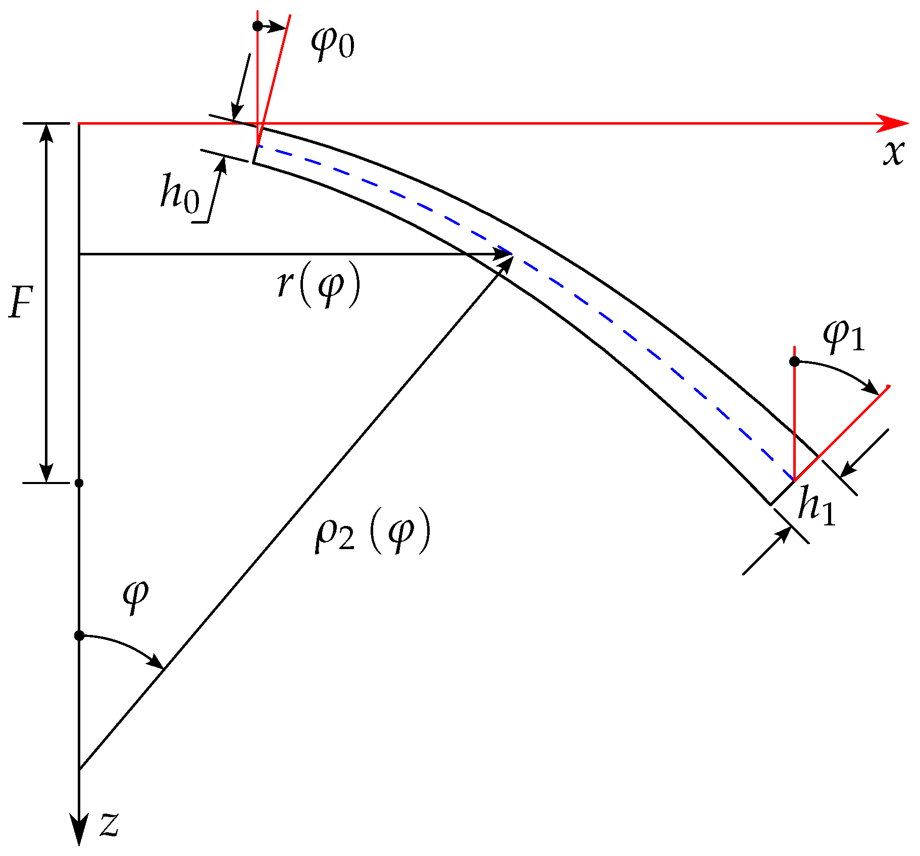
2.1. Geometrical Parameters
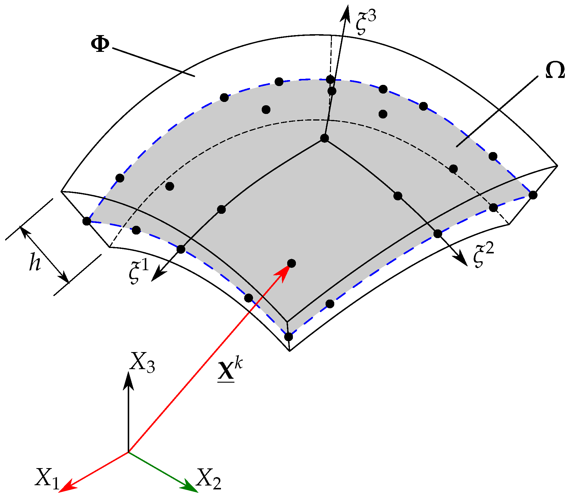
2.2. Displacement Field
2.3. Strains
3. Constitutive Equations
4. Equations of Motion
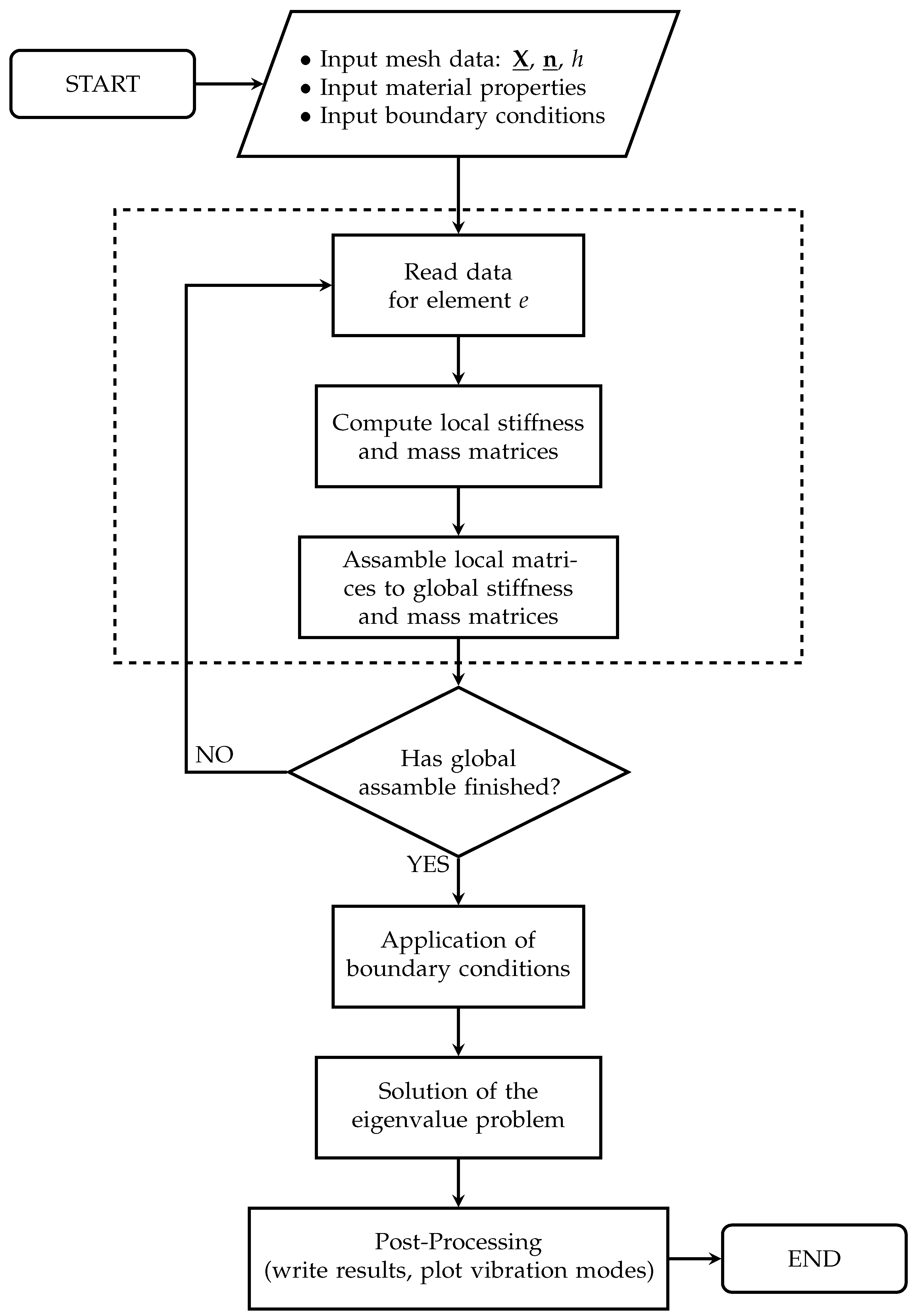
5. Finite Element Model
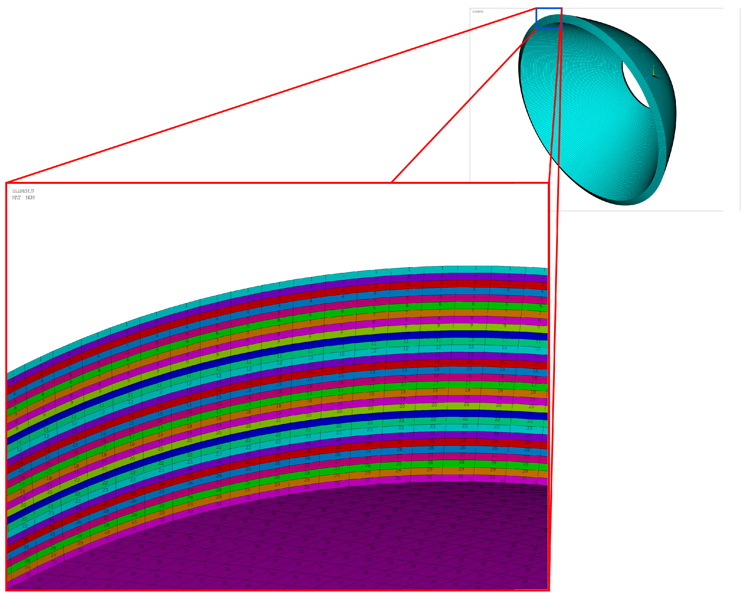
6. Solid Model
- Clamped edge: all the degrees of freedom of the nodes associated with the corresponding edge are constrained.
- Simply supported edge: all the degrees of freedom for the nodes located at the mid-surface of the solid model are constrained, and the remaining nodes are constrained in the tangential and the thickness directions.
7. Results
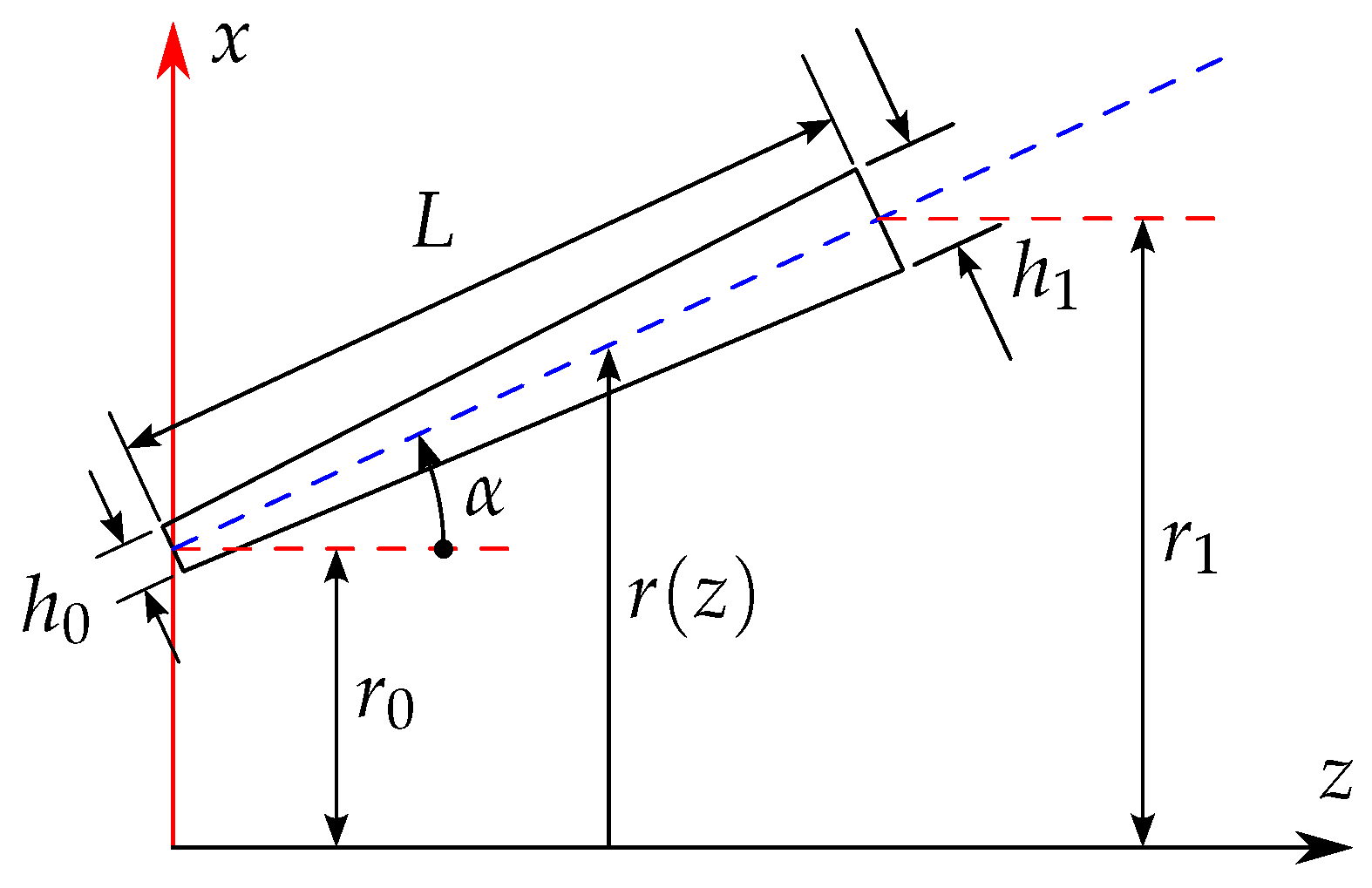
7.1. Geometrical Parameters
- 1.
- Conical shell
- Mid-surface:where .
- Thickness variation:
- 2.
- Cylindrical shell
- Mid-surface:
- Thickness variation:
- 3.
- Parabolic shell
- Thickness variation:
- 4.
- Hemispherical shell
- Mid-surface:
- Thickness variation:
7.2. Boundary Conditions
7.3. Material Properties
- Aluminum: GPa, kg/m, ;
- Zirconia: GPa, kg/m, .
7.4. Convergence Study
7.5. Numerical Verification
7.6. Numerical Results
8. Conclusions
- A finite element model for the linear vibration analysis, using spectral/hp elements based on a seven-parameter shell formulation, is extended to study functionally graded shells.
- Comparisons with the numerical results of a simulation using solid elements verify the performance of the present formulation. In addition, the comparisons suggest that the present formulation shows a better behavior for the modeling of conical, cylindrical, and parabolic shells subjected to the boundary conditions considered herein.
- In general, although the relative errors are between and obtained in the study of hemispherical shells, the present formulation has a good behavior for moderately thick to thin shells. It must be recalled that mechanical properties through the thickness of the 3D model are approximated using several layers in this direction. On the other hand, in the studies reported using the present formulation, the variation of the mechanical properties is evaluated using several Gauss-points while numerical integration through thickness is made, resulting in a closer approximation of them. For the aforementioned reasons, some differences between results, but a similar behavior, can be expected.
- Studying the effect of the power-law index on the free vibration response is relevant since, for a given thick or thin shell and boundary conditions, its response may be stiffer or not as the power-law index increases.
- Finally, the spectral/hp seven-parameter formulation used in the present finite element model allows a straightforward implementation of the FGM behavior and the use of three-dimensional constitutive equations. These features allow the use of considerably fewer elements, and therefore computational time, to model FG shell structures, when compared with models made of solid elements.
Author Contributions
Funding
Institutional Review Board Statement
Informed Consent Statement
Data Availability Statement
Conflicts of Interest
Abbreviations and Nomenclature
| Abbreviations | |
| FGM | Functionally graded material |
| FG | Functionally graded |
| FSDT | First-order shear deformation theory |
| TSDT | Third-order shear deformation theory |
| HSDT | Higher-order shear deformation theory |
| 3D | Three-dimensional |
| 2D | Two-dimensional |
| FG-I | Volume distribution of top constituent according to Equation (12) |
| FG-II | Volume distribution of top constituent according to Equation (13) |
| C | Clamped boundary condition |
| S | Simply supported boundary condition |
| F | Free edge boundary condition |
| UT | Uniform or constant thickness |
| LVT | Linear variable thickness |
| Nomenclature | |
| 3D geometry of the shell element | |
| Shell’s mid-surface | |
| Direction i of the curvilinear coordinates | |
| p | Polynomial order |
| 2D Lagrange interpolation function of order p | |
| Position vector of k-th spectral node | |
| Unit normal vector of the k-th spectral node | |
| h | Thickness at the k-th spectral node position |
| q | Number of spectral nodes per element |
| First derivative with respect | |
| Set of covariant basis vectors | |
| Jacobian matrix | |
| J | Determinant of the Jacobian matrix |
| Set of contravariant basis vectors | |
| Vector of the mid-surface displacements | |
| Difference vector | |
| Seventh parameter | |
| Green–Lagrange strain tensor | |
| Strain covariant component | |
| Strain covariant component associated with constant terms according to | |
| Strain covariant component associated with linear terms according to | |
| n | Volume fraction exponent or power-law index |
| Volume distribution of the top constituent following the power-law form i | |
| Contravariant components of the fourth-order elasticity tensor | |
| Lamé parameters as a function of | |
| Contravariant components of the Riemannian metric tensor | |
| Partial derivative with respect to time | |
| Mass inertia | |
| Effective extensional fourth-order stiffness tensor component | |
| Effective extensional–bending coupling fourth-order stiffness tensor component | |
| Effective bending fourth-order stiffness tensor component | |
| Frequency of natural vibration | |
| Vibration mode vector of the element e | |
| Average thickness | |
Appendix A. Convergence Study

| Natural Frequency | |||||||||||
|---|---|---|---|---|---|---|---|---|---|---|---|
| Size | |||||||||||
| UT | |||||||||||
| 0.6 | 4 | 206.3399 | 206.3406 | 228.7445 | 228.7594 | 307.8573 | 310.0378 | 318.3083 | 318.3083 | 349.2583 | 349.2601 |
| 16 | 206.2043 | 206.2043 | 225.9955 | 225.9955 | 279.1271 | 279.1425 | 318.2458 | 318.2458 | 349.0163 | 349.0163 | |
| 25 | 206.1950 | 206.1950 | 225.9754 | 225.9754 | 279.0831 | 279.0831 | 318.2343 | 318.2343 | 348.9862 | 348.9862 | |
| 36 | 206.1895 | 206.1895 | 225.9625 | 225.9625 | 279.0604 | 279.0604 | 318.2267 | 318.2267 | 348.9669 | 348.9669 | |
| 1 | 4 | 205.2655 | 205.2661 | 227.6316 | 227.6455 | 306.4297 | 308.6182 | 316.4647 | 316.4647 | 347.4014 | 347.4036 |
| 16 | 205.1328 | 205.1328 | 224.9006 | 224.9006 | 277.8596 | 277.8751 | 316.4039 | 316.4039 | 347.1603 | 347.1603 | |
| 25 | 205.1241 | 205.1241 | 224.8809 | 224.8809 | 277.8168 | 277.8168 | 316.3927 | 316.3927 | 347.1300 | 347.1300 | |
| 36 | 205.1192 | 205.1192 | 224.8691 | 224.8691 | 277.7954 | 277.7954 | 316.3855 | 316.3855 | 347.1107 | 347.1107 | |
| 5 | 4 | 204.3267 | 204.3273 | 230.8937 | 230.9606 | 309.7112 | 309.7112 | 313.8276 | 316.9194 | 346.9169 | 346.9202 |
| 16 | 204.1959 | 204.1959 | 228.1823 | 228.1823 | 285.6315 | 285.6461 | 309.6502 | 309.6502 | 346.6729 | 346.6729 | |
| 25 | 204.1866 | 204.1866 | 228.1618 | 228.1618 | 285.5871 | 285.5871 | 309.6392 | 309.6392 | 346.6426 | 346.6426 | |
| 36 | 204.1816 | 204.1816 | 228.149 | 228.149 | 285.5645 | 285.5645 | 309.6318 | 309.6318 | 346.6229 | 346.6229 | |
| VT | , , , | ||||||||||
| 0.6 | 4 | 64.2671 | 64.2683 | 72.8039 | 72.8039 | 77.7359 | 77.8637 | 82.4200 | 111.7707 | 112.4981 | 119.3929 |
| 16 | 64.2381 | 64.2383 | 72.7834 | 72.7834 | 77.1862 | 77.1862 | 82.3982 | 105.1581 | 105.1593 | 119.3415 | |
| 25 | 64.2342 | 64.2342 | 72.7792 | 72.7792 | 77.1813 | 77.1813 | 82.3935 | 105.1495 | 105.1496 | 119.3310 | |
| 36 | 64.2314 | 64.2316 | 72.7765 | 72.7765 | 77.1782 | 77.1782 | 82.3906 | 105.1451 | 105.1451 | 119.3240 | |
| 1 | 4 | 64.0133 | 64.0147 | 72.5720 | 72.5720 | 77.4079 | 77.5351 | 82.1966 | 111.3054 | 112.0354 | 118.9686 |
| 16 | 63.9856 | 63.9856 | 72.5516 | 72.5516 | 76.8608 | 76.8608 | 82.1739 | 104.7152 | 104.7165 | 118.9188 | |
| 25 | 63.9819 | 63.9819 | 72.5476 | 72.5476 | 76.8562 | 76.8562 | 82.1693 | 104.7070 | 104.7070 | 118.9087 | |
| 36 | 63.9793 | 63.9793 | 72.5448 | 72.5448 | 76.8531 | 76.8531 | 82.1662 | 104.7027 | 104.7027 | 118.9018 | |
| 5 | 4 | 64.7178 | 64.7191 | 71.8602 | 71.8604 | 79.7390 | 79.8619 | 80.9811 | 114.8458 | 115.4412 | 119.9444 |
| 16 | 64.6894 | 64.6896 | 71.8401 | 71.8401 | 79.1981 | 79.1981 | 80.9595 | 108.2964 | 108.2974 | 119.8919 | |
| 25 | 64.6855 | 64.6855 | 71.8360 | 71.8360 | 79.1933 | 79.1933 | 80.9551 | 108.2880 | 108.2880 | 119.8812 | |
| 36 | 64.6829 | 64.6829 | 71.8332 | 71.8332 | 79.1901 | 79.1901 | 80.9522 | 108.2835 | 108.2835 | 119.8740 | |
| Natural Frequency | |||||||||||
|---|---|---|---|---|---|---|---|---|---|---|---|
| Size | |||||||||||
| UT | |||||||||||
| 0.6 | 4 | 149.0672 | 149.0813 | 217.4327 | 220.1873 | 250.289 | 250.289 | 414.3378 | 421.2149 | 422.6686 | 431.4761 |
| 16 | 148.9533 | 148.9533 | 213.7694 | 213.7694 | 250.2324 | 250.2324 | 375.1731 | 375.2126 | 414.3378 | 418.8546 | |
| 25 | 148.9471 | 148.9471 | 213.7647 | 213.7647 | 250.2258 | 250.2258 | 375.1441 | 375.1441 | 414.3378 | 418.8213 | |
| 36 | 148.9438 | 148.9438 | 213.7629 | 213.7629 | 250.2222 | 250.2222 | 375.1404 | 375.1404 | 414.3378 | 418.8004 | |
| 1 | 4 | 148.1871 | 148.2012 | 216.6958 | 219.4371 | 248.6176 | 248.6176 | 411.5388 | 419.159 | 420.6086 | 430.1546 |
| 16 | 148.0766 | 148.0766 | 213.0478 | 213.0478 | 248.5642 | 248.5642 | 374.0646 | 374.1038 | 411.5388 | 416.811 | |
| 25 | 148.0712 | 148.0712 | 213.043 | 213.043 | 248.5585 | 248.5585 | 374.0361 | 374.0361 | 411.5388 | 416.7794 | |
| 36 | 148.0683 | 148.0683 | 213.0418 | 213.0418 | 248.5555 | 248.5555 | 374.0327 | 374.0327 | 411.5388 | 416.7596 | |
| 5 | 4 | 147.6200 | 147.6372 | 224.2188 | 226.9312 | 242.8096 | 242.8096 | 401.1873 | 424.5701 | 426.0516 | 445.3043 |
| 16 | 147.5116 | 147.5116 | 220.4488 | 220.4488 | 242.759 | 242.759 | 388.7491 | 388.7856 | 401.1873 | 422.1085 | |
| 25 | 147.5064 | 147.5064 | 220.4442 | 220.4442 | 242.7538 | 242.7538 | 388.7211 | 388.7211 | 401.1873 | 422.0764 | |
| 36 | 147.5035 | 147.5035 | 220.4425 | 220.4425 | 242.7507 | 242.7507 | 388.7175 | 388.7175 | 401.1873 | 422.0560 | |
| LVT | , , , | ||||||||||
| 0.6 | 4 | 58.5325 | 58.5403 | 79.1170 | 79.1170 | 97.4787 | 98.0998 | 125.2401 | 157.4556 | 157.4597 | 180.5150 |
| 16 | 58.5032 | 58.5035 | 79.1061 | 79.1061 | 96.1520 | 96.1520 | 125.2401 | 157.3938 | 157.3941 | 162.9478 | |
| 25 | 58.5015 | 58.5015 | 79.1040 | 79.1040 | 96.1511 | 96.1511 | 125.2401 | 157.3840 | 157.3840 | 162.9408 | |
| 36 | 58.5002 | 58.5004 | 79.1026 | 79.1026 | 96.1505 | 96.1505 | 125.2401 | 157.3773 | 157.3774 | 162.9400 | |
| 1 | 4 | 58.2046 | 58.2122 | 78.4490 | 78.4490 | 97.2474 | 97.8640 | 124.1085 | 156.6195 | 156.6236 | 179.9211 |
| 16 | 58.1765 | 58.1767 | 78.4397 | 78.4397 | 95.9248 | 95.9248 | 124.1085 | 156.5594 | 156.5598 | 162.6202 | |
| 25 | 58.1750 | 58.1750 | 78.4377 | 78.4377 | 95.9238 | 95.9238 | 124.1085 | 156.5500 | 156.5501 | 162.6132 | |
| 36 | 58.1739 | 58.1739 | 78.4366 | 78.4366 | 95.9233 | 95.9234 | 124.1085 | 156.5436 | 156.5437 | 162.6124 | |
| 5 | 4 | 58.8273 | 58.8348 | 76.8844 | 76.8844 | 100.5552 | 101.1290 | 120.9788 | 156.7878 | 156.7918 | 183.6858 |
| 16 | 58.7989 | 58.7991 | 76.8743 | 76.8743 | 99.2149 | 99.2149 | 120.9788 | 156.7283 | 156.7286 | 168.2562 | |
| 25 | 58.7974 | 58.7974 | 76.8723 | 76.8723 | 99.2141 | 99.2141 | 120.9788 | 156.7189 | 156.7189 | 168.2494 | |
| 36 | 58.7963 | 58.7963 | 76.8710 | 76.8710 | 99.2135 | 99.2137 | 120.9788 | 156.7125 | 156.7126 | 168.2487 | |
| Natural Frequency | |||||||||||
|---|---|---|---|---|---|---|---|---|---|---|---|
| Size | |||||||||||
| UT | |||||||||||
| 0.6 | 4 | 115.0771 | 115.0783 | 162.5836 | 162.5836 | 163.816 | 163.8276 | 190.6016 | 205.3549 | 205.3549 | 205.7548 |
| 16 | 115.0375 | 115.0375 | 162.5828 | 162.5828 | 162.6739 | 162.6739 | 190.6009 | 194.7506 | 194.7545 | 205.3518 | |
| 25 | 115.0374 | 115.0374 | 162.5828 | 162.5828 | 162.6739 | 162.6739 | 190.6009 | 194.7454 | 194.7454 | 205.3518 | |
| 36 | 115.0373 | 115.0373 | 162.5828 | 162.5828 | 162.6732 | 162.6732 | 190.6009 | 194.7448 | 194.7448 | 205.3518 | |
| 1 | 4 | 114.1884 | 114.1895 | 161.5536 | 161.5536 | 162.9672 | 162.9773 | 189.1796 | 203.9445 | 203.9445 | 204.8127 |
| 16 | 114.1494 | 114.1494 | 161.5521 | 161.5521 | 161.8309 | 161.8309 | 189.1789 | 193.8818 | 193.8857 | 203.9420 | |
| 25 | 114.1493 | 114.1493 | 161.5521 | 161.5521 | 161.8301 | 161.8301 | 189.1789 | 193.8772 | 193.8772 | 203.9420 | |
| 36 | 114.1492 | 114.1492 | 161.5521 | 161.5521 | 161.8301 | 161.8301 | 189.1789 | 193.8766 | 193.8766 | 203.9420 | |
| 5 | 4 | 114.1847 | 114.1854 | 157.9431 | 157.9431 | 162.9485 | 162.9594 | 186.2609 | 202.1293 | 202.1293 | 206.7551 |
| 16 | 114.1467 | 114.1467 | 157.9423 | 157.9423 | 161.8215 | 161.8215 | 186.2609 | 195.7845 | 195.7884 | 202.1268 | |
| 25 | 114.1466 | 114.1466 | 157.9423 | 157.9423 | 161.8207 | 161.8207 | 186.2602 | 195.7800 | 195.7800 | 202.1268 | |
| 36 | 114.1465 | 114.1465 | 157.9423 | 157.9423 | 161.8207 | 161.8207 | 186.2602 | 195.7793 | 195.7793 | 202.1262 | |
| LVT | , m, , , | ||||||||||
| 0.6 | 4 | 139.0314 | 139.0330 | 184.2228 | 184.5964 | 232.6821 | 232.6821 | 273.5517 | 277.8245 | 302.1489 | 302.1493 |
| 16 | 138.9795 | 138.9801 | 181.8076 | 181.8076 | 232.6816 | 232.6816 | 252.5840 | 252.5940 | 302.1124 | 302.1128 | |
| 25 | 138.9790 | 138.9790 | 181.8048 | 181.8048 | 232.6810 | 232.6816 | 252.5714 | 252.5714 | 302.1111 | 302.1111 | |
| 36 | 138.9782 | 138.9784 | 181.8041 | 181.8041 | 232.6810 | 232.6810 | 252.5694 | 252.5694 | 302.1111 | 302.1116 | |
| 1 | 4 | 137.4007 | 137.4023 | 182.9299 | 183.3013 | 230.7302 | 230.7302 | 271.8826 | 276.1198 | 300.6015 | 300.6019 |
| 16 | 137.3496 | 137.3502 | 180.5318 | 180.5318 | 230.7280 | 230.7280 | 251.0767 | 251.0868 | 300.5687 | 300.5691 | |
| 25 | 137.3490 | 137.3490 | 180.5297 | 180.5297 | 230.7280 | 230.7280 | 251.0646 | 251.0646 | 300.5674 | 300.5678 | |
| 36 | 137.3481 | 137.3482 | 180.5290 | 180.5290 | 230.7275 | 230.7280 | 251.0626 | 251.0631 | 300.5678 | 300.5678 | |
| 5 | 4 | 136.9053 | 136.9081 | 185.7905 | 186.1861 | 225.5277 | 225.5277 | 276.6422 | 281.0989 | 299.3446 | 299.3454 |
| 16 | 136.8544 | 136.8549 | 183.4657 | 183.4657 | 225.5265 | 225.5265 | 255.8724 | 255.8819 | 299.3099 | 299.3099 | |
| 25 | 136.8537 | 136.8538 | 183.4636 | 183.4636 | 225.5260 | 225.5265 | 255.8606 | 255.8606 | 299.3086 | 299.3086 | |
| 36 | 136.8530 | 136.8531 | 183.4629 | 183.4629 | 225.5260 | 225.5260 | 255.8591 | 255.8591 | 299.3086 | 299.3091 | |
| Natural Frequency | |||||||||||
|---|---|---|---|---|---|---|---|---|---|---|---|
| Size | |||||||||||
| UT | |||||||||||
| 0.6 | 4 | 142.9211 | 142.9228 | 208.2505 | 209.0329 | 286.9648 | 286.9648 | 371.2498 | 378.0133 | 379.8979 | 412.0659 |
| 16 | 142.7639 | 142.7639 | 204.6190 | 204.6190 | 286.8809 | 286.8809 | 335.2968 | 335.3127 | 379.7792 | 411.9857 | |
| 25 | 142.7490 | 142.7490 | 204.6141 | 204.6141 | 286.8646 | 286.8646 | 335.2817 | 335.2817 | 379.7558 | 411.9716 | |
| 36 | 142.7395 | 142.7395 | 204.6122 | 204.6122 | 286.8536 | 286.8536 | 335.2802 | 335.2802 | 379.7405 | 411.9624 | |
| 1 | 4 | 141.9287 | 141.9304 | 206.8133 | 207.592 | 284.9687 | 284.9687 | 368.682 | 375.4016 | 377.1949 | 409.1480 |
| 16 | 141.7716 | 141.7716 | 203.2066 | 203.2066 | 284.8847 | 284.8847 | 332.9832 | 332.9992 | 377.0763 | 409.0685 | |
| 25 | 141.7565 | 141.7565 | 203.2023 | 203.2023 | 284.8682 | 284.8682 | 332.9683 | 332.9683 | 377.0531 | 409.0542 | |
| 36 | 141.7468 | 141.7468 | 203.2004 | 203.2004 | 284.8576 | 284.8576 | 332.9668 | 332.9668 | 377.0377 | 409.0449 | |
| 5 | 4 | 141.5049 | 141.5083 | 211.0865 | 211.8818 | 278.8679 | 278.8679 | 370.0573 | 372.969 | 379.5433 | 401.4401 |
| 16 | 141.3544 | 141.3544 | 207.5792 | 207.5792 | 278.7852 | 278.7852 | 338.3654 | 338.3804 | 369.9389 | 401.3587 | |
| 25 | 141.3400 | 141.3400 | 207.5749 | 207.5749 | 278.7689 | 278.7689 | 338.3516 | 338.3516 | 369.9159 | 401.3441 | |
| 36 | 141.3306 | 141.3306 | 207.5731 | 207.5731 | 278.7584 | 278.7584 | 338.3505 | 338.3505 | 369.9005 | 401.3347 | |
| LVT | , m, , , | ||||||||||
| 0.6 | 4 | 213.8630 | 213.8719 | 282.1387 | 283.0775 | 348.9506 | 348.9506 | 465.8914 | 475.1184 | 479.0508 | 496.9698 |
| 16 | 213.7054 | 213.7054 | 278.8270 | 278.8270 | 348.8689 | 348.8689 | 428.3164 | 428.3294 | 478.9194 | 496.8319 | |
| 25 | 213.6865 | 213.6865 | 278.8166 | 278.8166 | 348.8526 | 348.8526 | 428.2966 | 428.2966 | 478.8930 | 496.8067 | |
| 36 | 213.6740 | 213.6740 | 278.8107 | 278.8107 | 348.8417 | 348.8417 | 428.2918 | 428.2918 | 478.8750 | 496.7901 | |
| 1 | 4 | 212.2336 | 212.2425 | 280.1837 | 281.1138 | 346.3059 | 346.3059 | 462.5427 | 471.6680 | 474.5570 | 492.2946 |
| 16 | 212.0760 | 212.0760 | 276.8967 | 276.8967 | 346.2251 | 346.2251 | 425.2914 | 425.3042 | 474.4270 | 492.1577 | |
| 25 | 212.0569 | 212.0569 | 276.8862 | 276.8862 | 346.2086 | 346.2086 | 425.2717 | 425.2717 | 474.4008 | 492.1327 | |
| 36 | 212.0443 | 212.0443 | 276.8807 | 276.8807 | 346.1977 | 346.1977 | 425.2672 | 425.2672 | 474.3832 | 492.1162 | |
| 5 | 4 | 213.8920 | 213.9015 | 287.5137 | 288.4290 | 340.3234 | 340.3234 | 471.6913 | 472.2575 | 480.9917 | 490.4160 |
| 16 | 213.7380 | 213.7380 | 284.2981 | 284.2981 | 340.2437 | 340.2437 | 435.4306 | 435.4425 | 471.5627 | 490.2747 | |
| 25 | 213.7191 | 213.7191 | 284.2879 | 284.2879 | 340.2277 | 340.2277 | 435.4117 | 435.4117 | 471.5366 | 490.2486 | |
| 36 | 213.7066 | 213.7066 | 284.2821 | 284.2821 | 340.2169 | 340.2169 | 435.4067 | 435.4067 | 471.5192 | 490.2313 | |
References
- Shen, H.S. Functionally Graded Materials: Nonlinear Analysis of Plates and Shells; CRC Press: Boca Raton, FL, USA, 2016. [Google Scholar]
- Mahamood, R.M.; Akinlabi, E.T. Introduction to functionally graded materials. In Functionally Graded Materials; Springer: Berlin/Heidelberg, Germany, 2017; pp. 1–8. [Google Scholar]
- Gupta, A.; Talha, M. Recent development in modeling and analysis of functionally graded materials and structures. Prog. Aerosp. Sci. 2015, 79, 1–14. [Google Scholar] [CrossRef]
- Punera, D.; Kant, T. A critical review of stress and vibration analyses of functionally graded shell structures. Compos. Struct. 2019, 210, 787–809. [Google Scholar] [CrossRef]
- Jha, D.K.; Kant, T.; Singh, R.K. A critical review of recent research on functionally graded plates. Compos. Struct. 2013, 96, 833–849. [Google Scholar] [CrossRef]
- Zhou, W.; Ai, S.; Chen, M.; Zhang, R.; He, R.; Pei, Y.; Fang, D. Preparation and thermodynamic analysis of the porous ZrO2/(ZrO2 + Ni) functionally graded bolted joint. Compos. Part B Eng. 2015, 82, 13–22. [Google Scholar] [CrossRef]
- Zhou, W.; Ai, S.; He, R.; Pei, Y.; Fang, D. Load distribution in threads of porous metal–ceramic functionally graded composite joints subjected to thermomechanical loading. Compos. Struct. 2015, 134, 680–688. [Google Scholar] [CrossRef]
- Sofiyev, A.H. A review of reasearch on the vibration and buckling of the FGM conical shells. Compos. Struct. 2019, 211, 301–317. [Google Scholar] [CrossRef]
- Dong, C.Y. Three-dimensional free vibration analysis of functionally graded annular plates using the Chebyshev–Ritz method. Mater. Des. 2008, 29, 1518–1525. [Google Scholar] [CrossRef]
- Talha, M.; Singh, B.N. Static response and free vibration analysis of FGM plates using higher order shear deformation theory. Appl. Math. Model. 2010, 34, 3991–4011. [Google Scholar] [CrossRef]
- Neves, A.M.A.; Ferreira, A.J.M.; Carrera, E.; Cinefra, M.; Roque, C.M.C.; Jorge, R.M.N.; Soares, C.M. Static, free vibration and buckling analysis of isotropic and sandwich functionally graded plates using a quasi-3D higher-order shear deformation theory and a meshless technique. Compos. Part B Eng. 2013, 44, 657–674. [Google Scholar] [CrossRef]
- Thai, H.T.; Vo, T.P. A new sinusoidal shear deformation theory for bending, buckling, and vibration of functionally graded plates. Appl. Math. Model. 2013, 37, 3269–3281. [Google Scholar] [CrossRef]
- Ramu, I.; Mohanty, S.C. Modal analysis of functionally graded material plates using finite element method. Procedia Mater. Sci. 2014, 6, 460–467. [Google Scholar] [CrossRef]
- Ghashochi-Bargh, H.; Razavi, S. A simple analytical model for free vibration of orthotropic and functionally graded rectangular plates. Alex. Eng. J. 2018, 57, 595–607. [Google Scholar] [CrossRef]
- Katili, I.; Batoz, J.L.; Maknun, I.J.; Katili, A.M. On static and free vibration analysis of FGM plates using an efficient quadrilateral finite element based on DSPM. Compos. Struct. 2021, 261, 113514. [Google Scholar] [CrossRef]
- Vinh, P.V.; Dung, N.T.; Tho, N.C.; Thom, D.V.; Hoa, L.K. Modified single variable shear deformation plate theory for free vibration analysis of rectangular FGM plates. Structures 2021, 29, 1435–1444. [Google Scholar] [CrossRef]
- Wang, X.; Jin, C.; Yuan, Z. Free vibration of FGM annular sectorial plates with arbitrary boundary supports and large sector angles. Mech. Based Des. Struct. Mach. 2022, 50, 331–351. [Google Scholar] [CrossRef]
- Efraim, E.; Eisenberger, M. Exact vibration analysis of variable thickness thick annular isotropic and FGM plates. J. Sound Vib. 2007, 299, 720–738. [Google Scholar] [CrossRef]
- Temel, B.; Noori, A.R. A unified solution for the vibration analysis of two-directional functionally graded axisymmetric Mindlin–Reissner plates with variable thickness. Int. J. Mech. Sci. 2020, 174, 105471. [Google Scholar] [CrossRef]
- Kumar, V.; Singh, S.J.; Saran, V.H.; Harsha, S.P. An analytical framework for rectangular FGM tapered plate resting on the elastic foundation. Mater. Today Proc. 2020, 28, 1719–1726. [Google Scholar] [CrossRef]
- Matsunaga, H. Free vibration and stability of functionally graded circular cylindrical shells accorinding to a 2D higher-order deformation theory. Compos. Struct. 2009, 88, 519–531. [Google Scholar] [CrossRef]
- Tornabene, F.; Viola, E.; Inman, D.J. 2-D differential quadrature solution for vibration analysis of functionally graded conical, cylindrical shell and annular plate structures. J. Sound Vib. 2009, 328, 259–290. [Google Scholar] [CrossRef]
- Tornabene, F.; Viola, E. Free vibration analysis of functionally graded panels and shells of revolution. Meccanica 2009, 44, 255–281. [Google Scholar] [CrossRef]
- Iqbal, Z.; Naeem, M.N.; Sultana, N. Vibration characteristics of FGM circular cylindrical shells using wave propagation approach. Acta Mech. 2009, 208, 237–248. [Google Scholar] [CrossRef]
- Neves, A.M.A.; Ferreira, A.J.M.; Carrera, E.; Cinefra, M.; Roque, C.M.C.; Jorge, R.M.N.; Soares, C.M.M. Free vibration analysis of functionally graded shells by a higher-order shear deformation theory and radial basis functions collocation, accounting for through-the-thickness deformations. Eur. J. Mech. A/Solids 2013, 37, 24–34. [Google Scholar] [CrossRef]
- Su, Z.; Jin, G.; Shi, S.; Ye, T. A unified accurate solution for vibration analysis of arbitrary functionally graded spherical shell segments with general boundary conditions. Compos. Struct. 2014, 111, 271–284. [Google Scholar] [CrossRef]
- Su, Z.; Jin, G.; Shi, S.; Ye, T.; Jia, X. A unified solution for vibration analysis of functionally graded cylindrical, conical shells and annular plates with general boundary conditions. Int. J. Mech. Sci. 2014, 80, 62–80. [Google Scholar] [CrossRef]
- Su, Z.; Jin, G.; Ye, T. Three-dimensional vibration analysis of thick functionally graded conical, cylindrical shell and annular plate structures with arbitrary elastic restraints. Compos. Struct. 2014, 118, 432–447. [Google Scholar] [CrossRef]
- Torabi, J.; Ansari, R. A higher-order isoparametric superelement for free vibration analysis of functionally graded shells of revolution. Thin-Walled Struct. 2018, 133, 169–179. [Google Scholar] [CrossRef]
- Ersoy, H.; Mercan, K.; Civalek, Ö. Frequencies of FGM shells and annular plates by the methods of discrete singular convolution and differential quadrature methods. Compos. Struct. 2018, 183, 7–20. [Google Scholar] [CrossRef]
- Brischetto, S. Exponential matrix method for the solution of exact 3D equilibrium equations for free vibrations of functionally graded plates and shells. J. Sandw. Struct. Mater. 2019, 21, 77–114. [Google Scholar] [CrossRef]
- Pham, T.D.; Pham, Q.H.; Phan, V.D.; Nguyen, H.N.; Do, V.T. Free vibration analysis of functionally graded shells using an edge-based smoothed finite element method. Symmetry 2019, 11, 684. [Google Scholar] [CrossRef]
- Moita, J.S.; Araújo, A.L.; Correia, V.F.; Mota Soares, C.a.M. Vibrations of Functionally Graded Material Axisymmetric Shells. Compos. Struct. 2020, 248, 112489. [Google Scholar] [CrossRef]
- Zannon, M.; Abu-Rqayiq, A.; Al-bdour, A. Free vibration analysis of thick FGM spherical shells based on a third-order shear deformation theory. Eur. J. Pure Appl. Math. 2020, 13, 766–778. [Google Scholar] [CrossRef]
- Bagheri, H.; Kiani, Y.; Eslami, M.R. Free vibration of FGM conical–spherical shells. Thin-Walled Struct. 2021, 160, 107387. [Google Scholar] [CrossRef]
- Li, H.; Pang, F.; Gong, Q.; Teng, Y. Free vibration analysis of axisymmetric functionally graded doubly-curved shells with un-uniform thickness distribution based on Ritz method. Compos. Struct. 2019, 225, 111145. [Google Scholar] [CrossRef]
- Gong, Q.; Li, H.; Chen, H.; Teng, Y.; Wang, N. Application of Ritz method for vibration analysis of stepped functionally graded spherical torus shell with general boundary conditions. Compos. Struct. 2020, 243, 112215. [Google Scholar] [CrossRef]
- Tornabene, F.; Fantuzzi, N.; Bacciocchi, M. Free vibrations of free-form doubly-curved shells made of functionally graded materials using higher-order equivalent single layer theories. Compos. Part B Eng. 2014, 67, 490–509. [Google Scholar] [CrossRef]
- Tornabene, F.; Fantuzzi, N.; Bacciocchi, M.; Viola, E.; Reddy, J.N. A numerical investigation on the natural frequencies of FGM sandwich shells with variable thickness by the Local Generalized Differential Quadrature Method. Appl. Sci. 2017, 7, 131. [Google Scholar] [CrossRef]
- Rao, D.K.; Blessington, P.J.; Tarapada, R. Finite Element Modeling and Analysis of Funcionally Graded (FG) Composite Shell Structures. Procedia Eng. 2012, 38, 3192–3199. [Google Scholar] [CrossRef]
- Mouli, B.C.; Kar, V.; Ramji, K.; Rajesh, M. Free vibration of functionally graded conical shell. Mater. Today Proc. 2018, 5, 14302–14308. [Google Scholar] [CrossRef]
- Marzavan, S.; Nastasescu, V. Free vibration analysis of a functionally graded plate by finite element method. Ain Shams Eng. J. 2023, 14, 102024. [Google Scholar] [CrossRef]
- Burlayenko, V.N.; Sadowski, T.; Altenbach, H.; Dimitrova, S. Three-Dimensional Finite Element Modelling of Free Vibrations of Functionally Graded Sanwhich Panels. In Recent Developments in the Theory of Shells; Springer: Berlin/Heidelberg, Germany, 2019; pp. 157–177. [Google Scholar]
- Bischoff, M.; Ramm, E. Shear deformable shell elements for large strains and rotations. Int. J. Numer. Methods Eng. 1997, 40, 4427–4449. [Google Scholar] [CrossRef]
- Hahn, Y.; Kikuchi, N. Mixed shell element for seven-parameter formulation. Int. J. Numer. Methods Eng. 2005, 64, 95–124. [Google Scholar] [CrossRef][Green Version]
- Arciniega, R.A.; Reddy, J.N. Tensor-based finite element formulation for geometrically nonlinear analysis of shell structures. Comput. Methods Appl. Mech. Eng. 2007, 196, 1048–1073. [Google Scholar] [CrossRef]
- Payette, G.S.; Reddy, J.N. A seven-parameter spectral/hp finite element formulation for isotropic, laminated composite and functionally graded shell structures. Comput. Methods Appl. Mech. Eng. 2014, 278, 664–704. [Google Scholar] [CrossRef]
- Gutierrez Rivera, M.; Reddy, J.N. Stress analysis of functionally graded shells using a 7-parameter shell element. Mech. Res. Commun. 2016, 78, 60–70. [Google Scholar] [CrossRef]
- Valencia Murillo, C.; Gutierrez Rivera, M.; Reddy, J.N. Linear Vibration Analysis of Shells Using a Seven-Parameter Spectral/hp Finite Element Model. Appl. Sci. 2020, 10, 5102. [Google Scholar] [CrossRef]
- Sansour, C. A theory and finite element formulation of shells at finite deformations involving thickness change: Circumventing the use of a rotation tensor. Arch. Appl. Mech. 1995, 65, 194–216. [Google Scholar] [CrossRef]
- Praveen, G.N.; Reddy, J.N. Nonlinear transient thermoelastic analysis of functionally graded ceramic-metal plates. Int. J. Solids Struct. 1998, 35, 4457–4476. [Google Scholar] [CrossRef]
- Reddy, J.N. Energy Principles and Variational Methods in Applied Mechanics, 2nd ed.; John Wiley & Sons: Hoboken, NJ, USA, 2002. [Google Scholar]
- Reddy, J.N. An Introduction to the Finite Element Method, 3rd ed.; McGraw-Hill: New York, NY, USA, 2005. [Google Scholar]
- Guennebaud, G.; Jacob, B.; Avery, P.; Bachrach, A.; Barthelemy, S. Eigen v3. 2010. Available online: http://eigen.tuxfamily.org (accessed on 24 September 2023).
- Leissa, A.W.; Kang, J.H. Three-dimensional vibration analysis of paraboloidal shells. JSME Int. J. Ser. Mech. Syst. Mach. Elem. Manuf. 2002, 45, 2–7. [Google Scholar] [CrossRef]


| Natural Frequency | |||||||||
|---|---|---|---|---|---|---|---|---|---|
| Model | – | – | – | – | – | – | – | ||
| 0.6 | 7-PL | 206.20 | 225.98 | 279.08 | 318.23 | 348.99 | 355.98 | 398.53 | 444.36 |
| 3D * | 205.93 | 226.02 | 279.55 | 318.32 | 348.57 | 356.80 | 397.36 | 444.55 | |
| FSDT [22] | 205.96 | 225.52 | 277.93 | 318.18 | 349.48 | - | - | - | |
| 1 | 7-PL | 205.12 | 224.88 | 277.82 | 316.39 | 347.13 | 354.42 | 396.71 | 441.88 |
| 3D * | 204.79 | 224.81 | 278.08 | 316.47 | 346.59 | 354.94 | 395.26 | 442.02 | |
| FSDT [22] | 204.91 | 224.44 | 276.66 | 316.32 | 347.66 | - | - | - | |
| 5 | 7-PL | 204.19 | 228.16 | 285.59 | 309.64 | 346.64 | 366.47 | 404.55 | 434.38 |
| 3D * | 203.69 | 227.75 | 285.14 | 309.65 | 345.64 | 365.74 | 402.10 | 434.30 | |
| FSDT [22] | 203.93 | 227.67 | 284.26 | 309.57 | 347.08 | - | - | - | |
| Natural Frequency | |||||||||
|---|---|---|---|---|---|---|---|---|---|
| Model | – | – | – | – | – | – | – | ||
| 0.6 | 7-PL | 148.95 | 213.76 | 250.23 | 375.14 | 414.34 | 418.82 | 454.43 | 523.52 |
| 3D * | 148.68 | 212.79 | 250.17 | 372.70 | 414.69 | 417.01 | 453.73 | 519.60 | |
| FSDT [22] | 150.03 | 212.94 | 250.74 | 370.63 | 415.47 | 420.39 | - | - | |
| 1 | 7-PL | 148.07 | 213.04 | 248.56 | 374.04 | 411.54 | 416.78 | 451.68 | 521.55 |
| 3D * | 147.74 | 211.83 | 248.49 | 371.09 | 411.89 | 414.67 | 450.87 | 517.02 | |
| FSDT [22] | 149.29 | 212.22 | 249.31 | 369.46 | 412.97 | 418.46 | - | - | |
| 5 | 7-PL | 147.51 | 220.44 | 242.75 | 388.72 | 401.19 | 422.08 | 446.11 | 537.48 |
| 3D * | 147.04 | 218.65 | 242.64 | 384.31 | 401.56 | 418.91 | 444.89 | 530.75 | |
| FSDT [22] | 148.75 | 219.49 | 243.43 | 383.71 | 402.56 | 423.57 | - | - | |
| Natural Frequency | |||||||||
|---|---|---|---|---|---|---|---|---|---|
| Model | – | – | – | – | – | ||||
| 0.6 | 7-PL | 115.04 | 162.58 | 162.67 | 190.60 | 194.75 | 194.75 | 205.35 | 218.29 |
| 3D * | 115.01 | 162.54 | 162.88 | 190.60 | 195.42 | 195.42 | 205.37 | 217.36 | |
| FSDT [23] | 115.40 | 162.85 | 165.07 | 193.28 | 193.28 | 196.66 | 210.82 | - | |
| 1 | 7-PL | 114.15 | 161.55 | 161.83 | 189.18 | 193.88 | 193.88 | 203.94 | 217.37 |
| 3D * | 114.10 | 161.52 | 161.98 | 189.16 | 194.43 | 194.43 | 203.95 | 216.39 | |
| FSDT [23] | 114.49 | 161.95 | 164.01 | 192.32 | 192.32 | 195.22 | 209.38 | - | |
| 5 | 7-PL | 114.15 | 157.94 | 161.82 | 186.26 | 195.78 | 195.78 | 202.13 | 218.63 |
| 3D * | 113.98 | 157.87 | 161.79 | 186.15 | 196.02 | 196.02 | 201.99 | 217.16 | |
| FSDT [23] | 114.44 | 160.33 | 161.78 | 194.04 | 194.04 | 194.05 | 207.19 | - | |
| Model | Vibration Mode | |||||
|---|---|---|---|---|---|---|
| – | – | – | – | – | ||
| 7-PL | Hz | Hz | Hz | Hz | Hz | Hz |
| 3D | Hz | Hz | Hz | Hz | Hz | Hz |
| Natural Frequency | |||||||||
|---|---|---|---|---|---|---|---|---|---|
| Model | – | – | – | – | – | – | – | ||
| 0.6 | 7-PL | 142.75 | 204.61 | 286.86 | 335.28 | 379.76 | 411.97 | 450.15 | 457.29 |
| 3D * | 143.01 | 205.53 | 286.90 | 336.75 | 379.75 | 411.97 | 450.15 | 459.24 | |
| FSDT [23] | 142.56 | 204.01 | 286.77 | 334.14 | 379.53 | 411.83 | - | - | |
| 1 | 7-PL | 141.76 | 203.20 | 284.87 | 332.97 | 377.05 | 409.05 | 446.97 | 454.12 |
| 3D * | 142.01 | 204.09 | 284.89 | 334.38 | 377.04 | 409.05 | 446.96 | 456.00 | |
| FSDT [23] | 141.59 | 202.64 | 284.78 | 331.87 | 376.84 | 408.93 | - | - | |
| 5 | 7-PL | 141.34 | 207.57 | 278.77 | 338.35 | 369.92 | 401.34 | 440.98 | 456.69 |
| 3D * | 141.43 | 207.98 | 278.72 | 338.95 | 369.76 | 401.19 | 440.70 | 457.67 | |
| FSDT [23] | 141.14 | 206.90 | 278.68 | 337.12 | 369.68 | 401.19 | - | - | |
| 1 | 5 | 1 | 5 | |||||||||
| 7PL | 3D | 7PL | 3D | 7PL | 3D | 7PL | 3D | 7PL | 3D | 7PL | 3D | |
| – | 101.96 | 99.10 | 101.58 | 98.62 | 103.00 | 99.57 | 88.96 | 86.55 | 88.61 | 86.12 | 90.34 | 87.46 |
| – | 125.12 | 124.75 | 124.38 | 124.02 | 121.97 | 121.50 | 93.71 | 92.40 | 93.41 | 91.98 | 92.86 | 91.27 |
| 160.29 | 155.02 | 159.92 | 154.34 | 164.31 | 157.48 | 106.33 | 105.18 | 106.04 | 104.73 | 104.82 | 103.43 | |
| 160.29 | 155.02 | 159.92 | 154.34 | 164.31 | 157.48 | 120.96 | 117.73 | 120.49 | 117.11 | 124.14 | 119.97 | |
| 181.57 | 177.36 | 180.78 | 176.37 | 182.29 | 176.86 | 120.96 | 117.73 | 120.49 | 117.11 | 124.14 | 119.97 | |
| 181.57 | 177.36 | 180.78 | 176.37 | 182.29 | 176.86 | 154.15 | 151.57 | 153.71 | 150.91 | 153.15 | 149.78 | |
| 205.72 | 204.42 | 204.22 | 203.21 | 198.99 | 199.79 | 159.58 | 156.52 | 159.04 | 155.78 | 159.71 | 155.72 | |
| 205.91 | 204.42 | 204.77 | 203.21 | 201.79 | 199.86 | 159.58 | 156.52 | 159.04 | 155.78 | 159.71 | 155.72 | |
| 205.91 | 206.41 | 204.77 | 205.02 | 201.79 | 199.87 | 164.50 | 160.34 | 163.86 | 159.44 | 168.87 | 163.06 | |
| 207.73 | 206.85 | 207.01 | 205.99 | 202.72 | 201.65 | 164.50 | 160.34 | 163.86 | 159.44 | 168.87 | 163.06 | |
| Max. Error | - | - | - | - | - | - | ||||||
| 1 | 5 | 1 | 5 | |||||||||
| 7PL | 3D | 7PL | 3D | 7PL | 3D | 7PL | 3D | 7PL | 3D | 7PL | 3D | |
| – | 73.76 | 72.43 | 73.38 | 72.01 | 73.23 | 71.65 | 64.23 | 62.47 | 63.98 | 62.16 | 64.69 | 62.64 |
| – | 84.73 | 82.08 | 84.41 | 81.68 | 86.67 | 83.55 | 72.78 | 71.76 | 72.55 | 71.44 | 71.84 | 70.62 |
| – | 104.14 | 103.72 | 103.58 | 103.14 | 101.67 | 101.15 | 77.18 | 74.79 | 76.86 | 74.40 | 79.19 | 76.38 |
| 124.04 | 120.57 | 123.65 | 120.00 | 127.76 | 123.35 | 82.39 | 81.54 | 82.17 | 81.20 | 80.96 | 79.93 | |
| 124.04 | 120.57 | 123.65 | 120.00 | 127.76 | 123.35 | 105.15 | 102.48 | 104.71 | 101.93 | 108.29 | 104.89 | |
| 151.23 | 147.91 | 150.50 | 147.07 | 149.20 | 147.02 | 105.15 | 102.48 | 104.71 | 101.93 | 108.29 | 104.89 | |
| 151.23 | 147.91 | 150.50 | 147.07 | 151.13 | 147.02 | 119.33 | 115.18 | 118.91 | 114.62 | 119.88 | 114.99 | |
| 152.28 | 151.27 | 151.73 | 150.61 | 151.13 | 148.02 | 121.86 | 117.67 | 121.40 | 117.08 | 122.83 | 117.87 | |
| 156.70 | 152.27 | 156.02 | 151.42 | 158.92 | 153.33 | 121.86 | 117.67 | 121.40 | 117.08 | 122.83 | 117.87 | |
| Max. Error | - | - | - | - | - | - | ||||||
| 1 | 5 | 1 | 5 | |||||||||
| 7PL | 3D | 7PL | 3D | 7PL | 3D | 7PL | 3D | 7PL | 3D | 7PL | 3D | |
| – | 52.69 | 51.04 | 52.43 | 50.75 | 52.89 | 51.00 | 45.53 | 43.84 | 45.36 | 43.63 | 45.57 | 43.66 |
| – | 58.04 | 55.90 | 57.78 | 55.60 | 58.52 | 56.87 | 46.64 | 44.56 | 46.44 | 44.33 | 47.45 | 45.13 |
| – | 59.39 | 58.42 | 59.08 | 58.08 | 59.31 | 57.38 | 50.32 | 48.99 | 50.15 | 48.77 | 49.73 | 48.21 |
| 72.78 | 70.51 | 72.48 | 70.14 | 74.97 | 72.28 | 54.03 | 52.76 | 53.87 | 52.48 | 53.19 | 51.78 | |
| 72.78 | 70.51 | 72.48 | 70.14 | 74.98 | 72.28 | 54.96 | 52.76 | 54.71 | 52.48 | 56.50 | 54.00 | |
| 77.08 | 76.52 | 76.69 | 76.11 | 75.30 | 74.63 | 54.96 | 52.81 | 54.71 | 52.58 | 56.50 | 54.00 | |
| 77.08 | 76.52 | 76.69 | 76.11 | 75.30 | 74.63 | 68.97 | 66.86 | 68.65 | 66.49 | 71.16 | 68.65 | |
| 92.91 | 91.54 | 92.51 | 91.07 | 90.61 | 89.98 | 68.97 | 66.86 | 68.65 | 66.49 | 71.16 | 68.65 | |
| 93.83 | 91.54 | 93.45 | 91.07 | 96.85 | 93.97 | 87.13 | 85.17 | 86.73 | 84.70 | 89.95 | 87.44 | |
| Max. Error | - | - | - | - | - | - | ||||||
| Model | Vibration Mode | ||||||
|---|---|---|---|---|---|---|---|
| – | – | – | – | – | |||
| 7-PL | Hz | Hz | Hz | Hz | Hz | Hz | Hz |
| 3D | Hz | Hz | Hz | Hz | Hz | Hz | Hz |
| n | ||||||
|---|---|---|---|---|---|---|
| 1 | 5 | |||||
| 7PL | 3D | 7PL | 3D | 7PL | 3D | |
| – | 64.07 | 63.72 | 63.28 | 62.98 | 62.17 | 61.75 |
| 123.97 | 121.23 | 122.50 | 120.98 | 119.37 | 121.87 | |
| 129.65 | 121.23 | 129.78 | 120.98 | 134.06 | 124.17 | |
| 129.65 | 126.14 | 129.78 | 124.89 | 134.06 | 124.17 | |
| – | 191.89 | 191.01 | 190.34 | 189.49 | 186.81 | 185.65 |
| 203.99 | 203.77 | 202.46 | 202.23 | 197.49 | 197.18 | |
| – | 217.19 | 204.85 | 217.00 | 204.04 | 220.95 | 205.82 |
| 313.85 | 294.01 | 314.23 | 293.37 | 320.46 | 299.19 | |
| 313.85 | 294.01 | 314.23 | 293.37 | 323.41 | 299.19 | |
| Max. Error | - | - | - | |||
| n | ||||||
|---|---|---|---|---|---|---|
| 1 | 5 | |||||
| 7PL | 3D | 7PL | 3D | 7PL | 3D | |
| – | 58.50 | 56.58 | 58.17 | 56.21 | 58.80 | 56.58 |
| – | 79.10 | 78.91 | 78.44 | 78.29 | 76.87 | 76.63 |
| – | 96.15 | 92.18 | 95.92 | 91.81 | 99.21 | 94.57 |
| 125.24 | 125.97 | 124.11 | 124.94 | 120.98 | 121.83 | |
| – | 157.38 | 153.83 | 156.55 | 152.89 | 156.72 | 152.33 |
| – | 162.94 | 156.82 | 162.61 | 156.20 | 168.25 | 160.75 |
| – | 179.49 | 173.24 | 178.90 | 172.36 | 182.66 | 174.78 |
| Max. Error | - | - | - | |||
| n | ||||||
|---|---|---|---|---|---|---|
| 1 | 5 | |||||
| 7PL | 3D | 7PL | 3D | 7PL | 3D | |
| – | 48.37 | 46.58 | 48.11 | 46.30 | 48.72 | 46.67 |
| – | 54.00 | 53.11 | 53.65 | 52.75 | 53.14 | 52.09 |
| – | 58.00 | 55.57 | 57.75 | 55.28 | 59.51 | 56.76 |
| – | 76.64 | 75.27 | 76.13 | 74.90 | 74.61 | 74.25 |
| – | 78.00 | 76.34 | 77.70 | 75.84 | 80.52 | 77.33 |
| – | 104.59 | 101.58 | 104.20 | 101.09 | 108.05 | 104.37 |
| Max. Error | - | - | - | |||
| Model | Vibration Mode | |||||
|---|---|---|---|---|---|---|
| – | – | – | – | |||
| 7-PL | Hz | Hz | Hz | Hz | Hz | Hz |
| 3D | Hz | Hz | Hz | Hz | Hz | Hz |
| n | ||||||
|---|---|---|---|---|---|---|
| 1 | 5 | |||||
| 7PL | 3D | 7PL | 3D | 7PL | 3D | |
| – | 138.98 | 133.61 | 137.35 | 132.00 | 136.85 | 130.85 |
| – | 181.80 | 177.58 | 180.53 | 176.21 | 183.46 | 179.06 |
| – | 232.68 | 232.88 | 230.73 | 230.96 | 225.53 | 225.64 |
| – | 252.57 | 252.06 | 251.06 | 250.34 | 255.86 | 254.68 |
| – | 302.11 | 298.29 | 300.57 | 296.72 | 299.31 | 294.62 |
| – | 306.54 | 300.91 | 305.01 | 299.20 | 309.83 | 303.04 |
| Max. Error | - | - | - | |||
| n | ||||||
|---|---|---|---|---|---|---|
| 1 | 5 | |||||
| 7PL | 3D | 7PL | 3D | 7PL | 3D | |
| – | 119.48 | 115.77 | 118.64 | 114.89 | 118.94 | 116.41 |
| – | 122.05 | 119.91 | 120.77 | 118.66 | 120.81 | 116.84 |
| – | 172.76 | 172.33 | 171.76 | 171.22 | 173.29 | 172.75 |
| – | 208.23 | 210.71 | 207.04 | 209.37 | 209.48 | 211.53 |
| – | 228.63 | 227.59 | 227.39 | 226.31 | 223.38 | 223.67 |
| – | 230.51 | 230.82 | 228.80 | 229.13 | 225.88 | 224.48 |
| Max. Error | - | - | - | |||
| n | ||||||
|---|---|---|---|---|---|---|
| 1 | 5 | |||||
| 7PL | 3D | 7PL | 3D | 7PL | 3D | |
| – | 78.31 | 78.03 | 77.70 | 77.41 | 78.79 | 78.05 |
| – | 112.95 | 114.96 | 112.32 | 114.26 | 112.91 | 112.39 |
| – | 116.41 | 116.08 | 115.36 | 115.04 | 115.13 | 116.39 |
| – | 155.52 | 159.99 | 154.62 | 158.99 | 154.93 | 158.71 |
| – | 170.88 | 176.93 | 169.87 | 175.80 | 170.10 | 175.69 |
| – | 182.82 | 184.09 | 181.73 | 182.96 | 179.73 | 180.76 |
| Max. Error | - | - | - | |||
| Model | Vibration Mode | |||||
|---|---|---|---|---|---|---|
| – | – | – | – | – | – | |
| 7-PL | Hz | Hz | Hz | Hz | Hz | Hz |
| 3D | Hz | Hz | Hz | Hz | Hz | Hz |
| n | ||||||
|---|---|---|---|---|---|---|
| 1 | 5 | |||||
| 7PL | 3D | 7PL | 3D | 7PL | 3D | |
| – | 442.59 | 423.35 | 437.86 | 418.65 | 434.18 | 413.44 |
| – | 458.16 | 425.35 | 453.14 | 420.03 | 456.14 | 419.90 |
| 619.59 | 598.02 | 615.52 | 589.93 | 598.59 | 583.48 | |
| 634.79 | 626.47 | 625.45 | 621.43 | 620.69 | 605.34 | |
| – | 687.08 | 643.50 | 679.83 | 635.00 | 683.42 | 632.22 |
| 756.26 | 718.08 | 747.01 | 708.77 | 738.23 | 693.93 | |
| – | 774.88 | 721.68 | 763.24 | 711.05 | 757.58 | 699.82 |
| 906.26 | 881.70 | 899.18 | 868.81 | 874.43 | 854.77 | |
| Max. Error | - | - | - | |||
| n | ||||||
|---|---|---|---|---|---|---|
| 1 | 5 | |||||
| 7PL | 3D | 7PL | 3D | 7PL | 3D | |
| – | 312.90 | 292.48 | 310.07 | 289.79 | 315.58 | 293.36 |
| – | 382.61 | 375.14 | 379.14 | 371.83 | 375.03 | 366.38 |
| – | 461.50 | 433.85 | 457.54 | 429.81 | 467.90 | 437.24 |
| 563.95 | 542.00 | 556.87 | 536.10 | 550.30 | 528.42 | |
| 632.93 | 598.01 | 625.57 | 591.51 | 619.64 | 588.23 | |
| 632.93 | 598.02 | 625.57 | 591.51 | 626.45 | 588.23 | |
| 634.47 | 614.37 | 628.57 | 608.52 | 626.45 | 602.37 | |
| 639.65 | 642.00 | 635.46 | 637.34 | 626.63 | 621.72 | |
| 687.48 | 654.55 | 681.40 | 648.09 | 694.55 | 655.38 | |
| Max. Error | - | - | - | |||
| n | ||||||
|---|---|---|---|---|---|---|
| 1 | 5 | |||||
| 7PL | 3D | 7PL | 3D | 7PL | 3D | |
| – | 213.69 | 204.60 | 212.06 | 203.05 | 213.72 | 203.73 |
| – | 278.82 | 261.85 | 276.89 | 259.97 | 284.29 | 266.47 |
| – | 348.85 | 347.55 | 346.21 | 344.94 | 340.23 | 338.50 |
| – | 428.30 | 410.50 | 425.27 | 407.47 | 435.41 | 416.22 |
| 478.89 | 465.83 | 474.40 | 461.85 | 471.54 | 457.11 | |
| – | 496.81 | 482.31 | 492.13 | 478.18 | 490.25 | 474.15 |
| 541.01 | 522.79 | 536.21 | 518.42 | 538.24 | 517.91 | |
| Max. Error | - | - | - | |||
| n | ||||||
|---|---|---|---|---|---|---|
| 1 | 5 | |||||
| 7PL | 3D | 7PL | 3D | 7PL | 3D | |
| – | 166.08 | 156.34 | 165.07 | 155.34 | 165.93 | 159.11 |
| – | 168.36 | 165.52 | 167.19 | 164.37 | 169.40 | 162.67 |
| – | 258.15 | 247.58 | 256.59 | 246.01 | 263.57 | 252.32 |
| – | 330.83 | 331.02 | 328.56 | 328.75 | 321.87 | 321.89 |
| – | 368.54 | 359.67 | 366.25 | 357.34 | 375.09 | 365.31 |
| 422.31 | 419.84 | 419.00 | 416.72 | 412.14 | 409.15 | |
| – | 437.11 | 434.21 | 433.59 | 430.96 | 426.26 | 422.88 |
| Max. Error | - | - | - | |||
| Model | Vibration Mode | |||||
|---|---|---|---|---|---|---|
| – | – | – | – | – | ||
| 7-PL | Hz | Hz | Hz | Hz | Hz | Hz |
| 3D | Hz | Hz | Hz | Hz | Hz | Hz |
Disclaimer/Publisher’s Note: The statements, opinions and data contained in all publications are solely those of the individual author(s) and contributor(s) and not of MDPI and/or the editor(s). MDPI and/or the editor(s) disclaim responsibility for any injury to people or property resulting from any ideas, methods, instructions or products referred to in the content. |
© 2023 by the authors. Licensee MDPI, Basel, Switzerland. This article is an open access article distributed under the terms and conditions of the Creative Commons Attribution (CC BY) license (https://creativecommons.org/licenses/by/4.0/).
Share and Cite
Valencia Murillo, C.E.; Gutierrez Rivera, M.E.; Flores Samano, N.; Celaya Garcia, L.D. A Seven-Parameter Spectral/hp Finite Element Model for the Linear Vibration Analysis of Functionally Graded Shells with Nonuniform Thickness. Appl. Sci. 2023, 13, 11540. https://doi.org/10.3390/app132011540
Valencia Murillo CE, Gutierrez Rivera ME, Flores Samano N, Celaya Garcia LD. A Seven-Parameter Spectral/hp Finite Element Model for the Linear Vibration Analysis of Functionally Graded Shells with Nonuniform Thickness. Applied Sciences. 2023; 13(20):11540. https://doi.org/10.3390/app132011540
Chicago/Turabian StyleValencia Murillo, Carlos Enrique, Miguel Ernesto Gutierrez Rivera, Nicolas Flores Samano, and Luis David Celaya Garcia. 2023. "A Seven-Parameter Spectral/hp Finite Element Model for the Linear Vibration Analysis of Functionally Graded Shells with Nonuniform Thickness" Applied Sciences 13, no. 20: 11540. https://doi.org/10.3390/app132011540
APA StyleValencia Murillo, C. E., Gutierrez Rivera, M. E., Flores Samano, N., & Celaya Garcia, L. D. (2023). A Seven-Parameter Spectral/hp Finite Element Model for the Linear Vibration Analysis of Functionally Graded Shells with Nonuniform Thickness. Applied Sciences, 13(20), 11540. https://doi.org/10.3390/app132011540