Adaptive Locomotion Learning for Quadruped Robots by Combining DRL with a Cosine Oscillator Based Rhythm Controller

Abstract

Animals have evolved to adapt to complex and uncertain environments, acquiring locomotion skills for diverse surroundings. To endow a robot’s animal-like locomotion ability, in this paper, we propose a learning algorithm for quadruped robots based on deep reinforcement learning (DRL) and a rhythm controller that is based on a cosine oscillator. For a quadruped robot, two cosine oscillators are utilized at the hip joint and the knee joint of one leg, respectively, and, finally, eight oscillators form the controller to realize the quadruped robot’s locomotion rhythm during moving. The coupling between the cosine oscillators of the rhythm controller is realized by the phase difference, which is simpler and easier to realize when dealing with the complex coupling relationship between different joints. DRL is used to help learn the controller parameters and, in the reward function design, we address the challenge of terrain adaptation without relying on the complex camera-based vision processing but based on the proprioceptive information, where a state estimator is introduced to achieve the robot’s posture and help finally utilize the food-end coordinate. Experiments are carried out in CoppeliaSim, and all of the flat, uphill and downhill conditions are considered. The results show that the robot can successfully accomplish all the above skills and, at the same time, with the reward function designed, the robot’s pitch angle, yaw angle and roll angle are very small, which means that the robot is relatively stable during walking. Then, the robot is transplanted to a new scene; the results show that although the environment is previously unencountered, the robot can still fulfill the task, which demonstrates the effectiveness and robustness of this proposed method.

1. Introduction

Quadruped animals, shaped by billions of years of natural selection, possess remarkable environmental adaptability and robust control capabilities in coordinated motor tasks. Taking inspiration from nature, bioinspired legged robots have been developed. Quadruped robots offer greater terrain adaptability compared to wheeled and crawler robots, making them more efficient in disaster scenarios [1,2]. Additionally, quadruped robots offer superior stability compared to biped robots and require less complexity and energy than hexapod and octopod robots [3,4]. Due to these advantages, extensive research has focused on quadruped robots, with particular emphasis on motion control as it directly impacts their overall performance in various tasks.

In order to fulfill the motion control of the quadruped robot, many models have been proposed, such as the zero moment point (ZMP) control [5], model predictive control (MPC) [6], virtual model control (VMC) [7], etc. Zhang et al. [8] calculated the optimal trajectory of the hip joint based on the stability margin of ZMP and used inverse kinematics principles to determine the robot joint angles. The feasibility of the method was verified on the BIT robot. Du et al. [9] designed an objective function and constraints for MPC based on the quadruped robot’s motion model, enabling tilt and forward motion control. In addition to the above methods, the central pattern generator (CPG), a biological motor control mechanism resembling that of quadruped animals, is commonly employed for control tasks in quadruped robots.

Biological studies have revealed that the central pattern generator located in the spinal cord mainly controls the rhythmic movement of vertebrates, such as walking, running and jumping [10,11]. Building upon this knowledge, numerous CPG models have been proposed for motion control in legged robots. These models include the Matsuoka neuron oscillator [12], the Kimura model [13] and the Hopf oscillator model [14]. In 2014, Xiao et al. [14] designed a gait switch mechanism for quadruped robots based on the Hopf oscillator. Simulation results demonstrated the effectiveness of this approach. The robot could smoothly and rapidly realize the conversion between two gaits. In [15], environmental information was sensed by the robot’s sensors and a reflex model was centralized within the CPG network. This allowed the quadruped robot to seamlessly transition from flat ground to the slope. Zhang et al. [16] designed a series CPG model capable of generating arbitrary periodic signals and dynamically adjusting its phase online. They achieved trot gait on the baby elephant quadruped robot. In a more recent study by Zhang et al. in 2021 [17], a CPG network with complex-value parameters was designed based on the dynamics of the quadruped robot and, additionally, a DC motor was integrated into the CPG network, enabling the robot to perform uphill and downhill motions. Although CPG control has achieved certain results, its coupling is strong and complicated, which has certain restrictions on the robot’s movement, and its parameter tuning is also a complicated process.

Recently, the combination of deep learning (DL) and reinforcement learning (RL) has led to the emergence of deep reinforcement learning (DRL) techniques, which have found increasing applications in robotics [18,19,20]. Unlike model-based methods, DRL is an end-to-end model-free learning method that relies on trial-and-error exploration [21,22]. By interacting with the environment, robots utilizing DRL gain valuable experience and gradually learn optimal movement strategies based on a reward function, mirroring the learning process of infants acquiring walking skills. Researchers have applied DRL in various robotic tasks. Zhu et al. [23] combined DRL with foot trajectory planning to enable quadruped robots to traverse slopes. Lee et al. [24] designed a hierarchical reinforcement learning algorithm for climbing over obstacles. Bellegarda et al. [25] redefined an oscillator based on the amplitude-controlled phase oscillator, which generated swimming and walking behaviors in salamander robots [26], and used the Proximal Policy Optimization (PPO) algorithm to learn the oscillator parameters. Rudin et al. [27] used DRL algorithms to train robot jumping and landing, successfully transferring the learned skills to the SpaceBok robot. In 2021, Lee et al. [28] developed a control algorithm based on RL and the artificial neural network; the RL policy was determined according to the expected optimal motor angle of the quadruped robot, and the neural network was trained with this policy as training data, enabling self-balancing control of the robot. While DRL algorithms can facilitate the learning of various motor skills by robots, it is important to note that learning from scratch requires a large number of interactions between the robot and the environment to obtain sufficient training samples. Consequently, the learning process can be time-consuming.

In this paper, to mimic the properties of biorhythm movement, we propose a new kind of adaptive learning algorithm that combines deep reinforcement learning (DRL) and a rhythm controller based on a cosine oscillator for controlling the locomotion of a quadruped robot. The rhythm controller is responsible for coordinating the movements of the robot’s four legs, while DRL is employed to learn the parameters of the controller and enable the robot to acquire various motor skills. The main contributions of this paper are as follows:

(1)

Eight cosine oscillators are used to construct the quadruped robot’s locomotion rhythm controller, and then the coordination of different legs is coupled just by the phase relationship among the eight joints. This simple weak coupling has fewer restrictions on the robot movement, which makes the generation of legged robots’ locomotion rhythm simpler and easier, and it is also easy to realize all kinds of gaits, as well as applying to most kinds of legged robots.

(2)

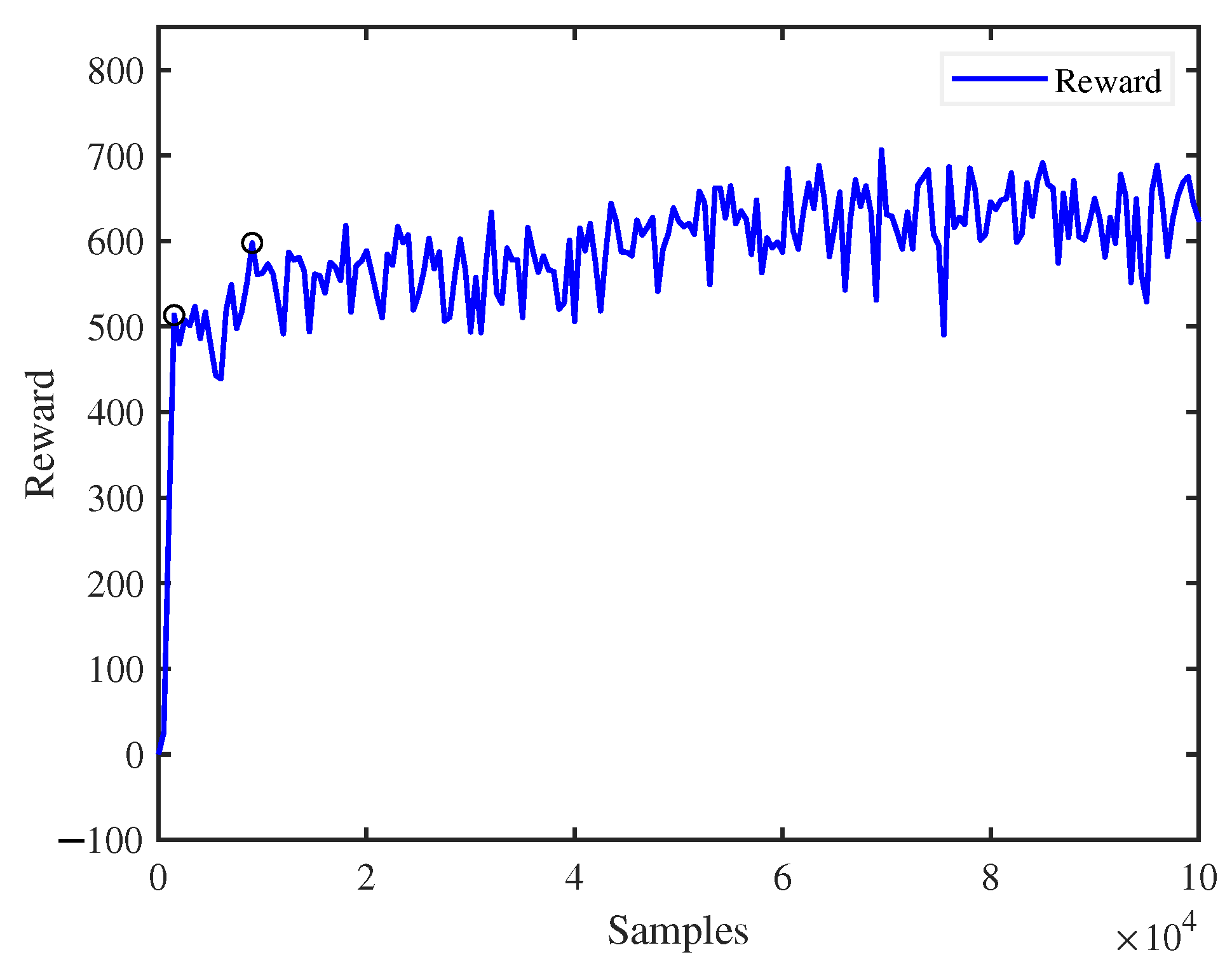
The Soft Actor-Critic (SAC), a kind of DRL algorithm, is used to train the parameters of the rhythm controller, which addresses the challenge of automatic acquisition and adjustment of the controller parameters. The reward function designed in this paper not only considers the robot’s general locomotion abilities, such as attitude balance and yaw control, but also takes its adaption to complex terrain into account. Therefore, a state estimation method is proposed, and the achieved slope information is integrated into the reward function to finally enable the robot to better cope with an unknown environment.

The rest of this paper is organized as follows. Section 2 introduces the concrete structure of the robot and the gait planning. Section 3 introduces quadruped robot locomotion learning algorithms in detail, including the rhythm controller based on a cosine oscillator, the slope information estimation method and the deep reinforcement learning algorithm. Section 4 shows the simulation results of the locomotion learning algorithm on the robot. Finally, Section 5 gives a brief conclusion.

2. The Robot

2.1. The Quadruped Robot

The quadruped robot used in this work is shown in Figure 1, which is 0.8 m long, 0.7 m wide and 0.732 m high. The robot has four legs, which are named left-front leg (LF), right-front leg (RF), left-back leg (LB) and right-back leg (RB). For each leg, two joints are considered, named the hip joint and the knee joint as shown in Figure 1.

The motion states of the quadruped robot include the position of the robot’s center of gravity ($x,y,z$), the orientations (pitch P, roll R and yaw Y), the velocities and accelerated velocities of the robot’s movement ($v_x,v_y,v_z,{\dot{v}}_x,{\dot{v}}_y,{\dot{v}}_z$), the foot endpoint positions (($x_{foot}^i,y_{foot}^i,z_{foot}^i$), where $i=1,2,3,4$), the joint angles (${\xi }_j$, where $j=1,2,\cdots ,7,8$) and the angular velocities (${\dot{\xi }}_j$).

2.2. Gait Planner

For quadruped robots, trot gait, space gait, bound gait, crawl gait and walk gait are often used [29]. In this work, the trot gait is chosen, of which the two diagonal legs of the quadruped robot always move in the same state, while the other two legs move in the opposite state; therefore, two legs of a quadruped robot are in the supporting state at any time. The trot gait movement process is shown in Figure 2; for example, at the beginning, RF and LB are in the swing phase in black, while LF and RB are in the support phase in white, after half a cycle, the swing phase and the support phase exchange.

3. Locomotion Learning Algorithm

In this paper, a quadruped robot adaptive locomotion learning control architecture algorithm is proposed, and the algorithm structure framework is shown in Figure 3. The algorithm mainly consists of the Soft Actor Critic (SAC) and a rhythm controller based on a cosine oscillator, in which four control units constitute the rhythm controller and directly output the angle required by the eight joints of the robot, while the SAC algorithm is used to learn the parameters required by the controller. In addition, in order to reduce the number of parameters of the controller, the trot gait is integrated into the rhythm controller. Moreover, in order to better adapt the robot to the irregular environment, a slope angle estimation method is proposed, and the angle information is considered in the reward function.

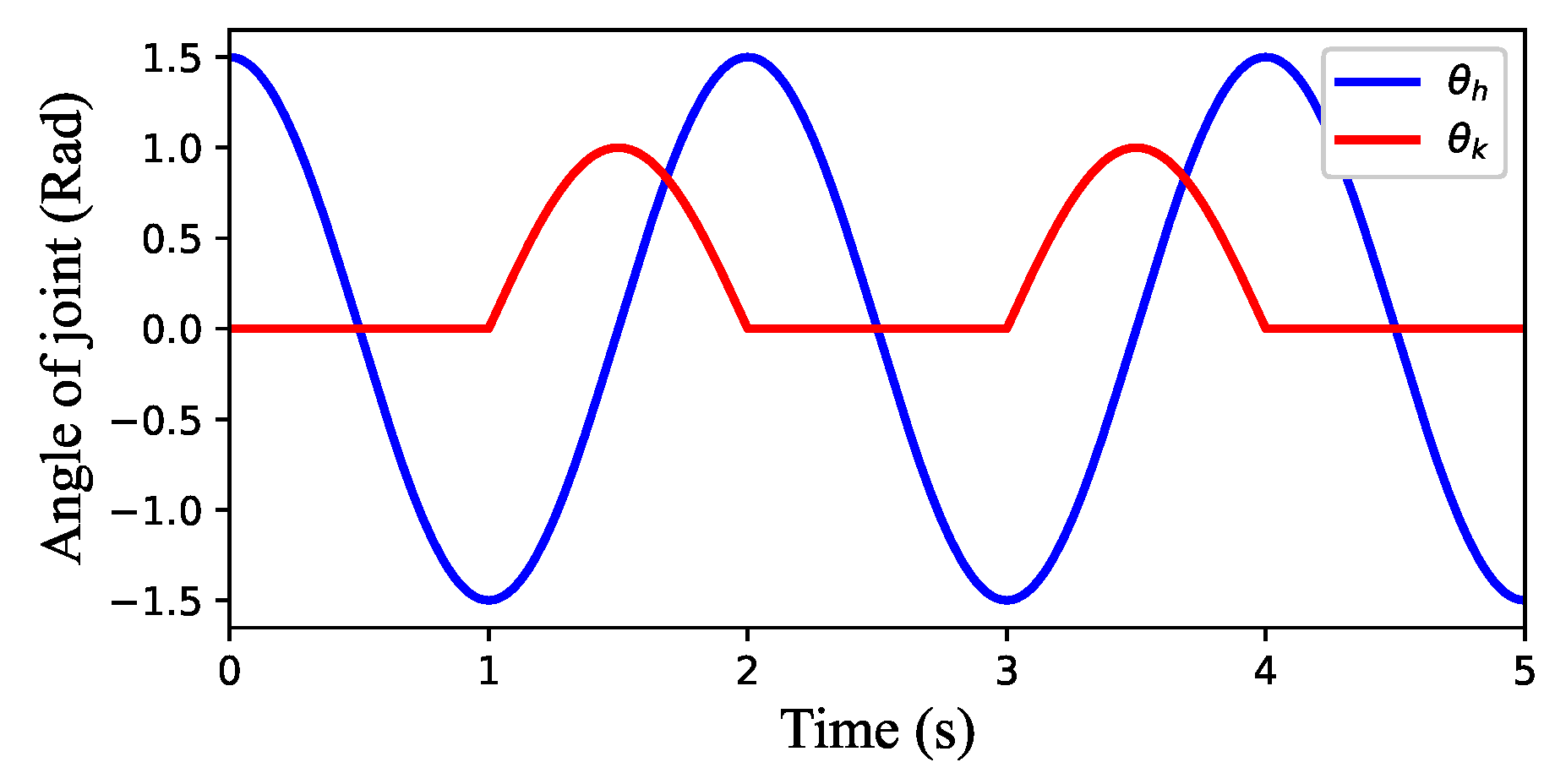
3.1. Rhythm Controller Based on a Cosine Oscillator

3.1.1. Single-Legged Control Unit

In this work, cosine oscillators [30] are used to make up the rhythm controller. Each leg of the quadruped robot is controlled by a control unit, which consists of N cosine oscillators; the equation for this is as follows:

$$\begin{array}{cc}\hfill Y_i& =A_{i}cos(\frac{2\pi t}{T}+{\phi }_i),\hfill \end{array}$$

(1)

where $Y_i$ represents the output of the ith oscillator, $A_i$ is the amplitude of the ith oscillator, T is the period of the oscillator, and ${\phi }_i$ is the initial phase of the oscillator.

It is pointed out that when one leg is in the support phase, it is better for the quadruped robot to move by swinging the hip back and keeping the knee motionless [31]. So, for the robot in this work with two joints on one leg, the control unit is designed as Equation (2):

$$\left\{\begin{array}{cc}{Y}_h\hfill & =A_{h}cos(\frac{2\pi t}{T}+{\phi }_0),\hfill \\ Y_k\hfill & =A_{k}cos(\frac{2\pi t}{T}+{\phi }_1),\hfill \\ {\theta }_h\hfill & =Y_h,\hfill \\ {\theta }_k\hfill & =\left\{\begin{array}{c}{Y}_k,\mathrm{if}{Y}_k\ge 0,\hfill \\ 0,\mathrm{if}{Y}_k<0,\hfill \end{array}\right.\hfill \end{array}\right.$$

(2)

where ${\theta }_h$ is the signal of the hip joint, ${\theta }_k$ is the signal of the knee joint, $A_h$ represents the amplitude of the hip joint and $A_k$ represents the amplitude of the knee joint. Figure 4 shows that the single-legged control unit output when $A_h=1.5$, $A_k=1.0$, $T=2.0$, ${\phi }_0=0$, ${\phi }_1=\frac{\pi }{2}$. It can be seen from the picture that the motion waveform of the hip joint is full wave and that of the knee joint is half wave. From $t=0$ to $t=\frac{T}{2}=1$, with one leg in the support phase, the hip rotates from 1.5 radians to −1.5 radians, and the knee does not move. From $t=\frac{T}{2}=1$ to $t=T=2$, with the leg in the swing phase, the hip rotates from −1.5 to 1.5 radians, the knee rotates from 0 to 1 radians and then from 1 to 0 radians.

3.1.2. Four-Legged Rhythm Controller

The rhythm controller, as shown in Figure 5, consists of four control units; the expression for this is shown in Equation (3):

$$\left\{\begin{array}{cc}{\theta }_h^{LF}\hfill & =A_{h}cos(\frac{2\pi t}{T}+{\phi }_0),\hfill \\ {\theta }_k^{LF}\hfill & =\left\{\begin{array}{c}{A}_{k}cos(\frac{2\pi t}{T}+{\phi }_1),\mathrm{if}{A}_{k}cos(\frac{2\pi t}{T}+{\phi }_1)\ge 0,\hfill \\ 0,\mathrm{if}{A}_{k}cos(\frac{2\pi t}{T}+{\phi }_1)<0.\hfill \end{array}\right.\hfill \\ {\theta }_h^{RF}\hfill & =A_{h}cos(\frac{2\pi t}{T}+{\phi }_2),\hfill \\ {\theta }_k^{RF}\hfill & =\left\{\begin{array}{c}{A}_{k}cos(\frac{2\pi t}{T}+{\phi }_3),\mathrm{if}{A}_{k}cos(\frac{2\pi t}{T}+{\phi }_3)\ge 0,\hfill \\ 0,\mathrm{if}{A}_{k}cos(\frac{2\pi t}{T}+{\phi }_3)<0.\hfill \end{array}\right.\hfill \\ {\theta }_h^{LB}\hfill & =A_{h}cos(\frac{2\pi t}{T}+{\phi }_4),\hfill \\ {\theta }_k^{LB}\hfill & =\left\{\begin{array}{c}{A}_{k}cos(\frac{2\pi t}{T}+{\phi }_5),\mathrm{if}{A}_{k}cos(\frac{2\pi t}{T}+{\phi }_5)\ge 0,\hfill \\ 0,\mathrm{if}{A}_{k}cos(\frac{2\pi t}{T}+{\phi }_5)<0.\hfill \end{array}\right.\hfill \\ {\theta }_h^{RB}\hfill & =A_{h}cos(\frac{2\pi t}{T}+{\phi }_6),\hfill \\ {\theta }_k^{RB}\hfill & =\left\{\begin{array}{c}{A}_{k}cos(\frac{2\pi t}{T}+{\phi }_7),\mathrm{if}{A}_{k}cos(\frac{2\pi t}{T}+{\phi }_7)\ge 0,\hfill \\ 0,\mathrm{if}{A}_{k}cos(\frac{2\pi t}{T}+{\phi }_7)<0,\hfill \end{array}\right.\hfill \end{array}\right.$$

(3)

where ${\theta }_h^{LF},{\theta }_k^{LF},{\theta }_h^{RF},{\theta }_k^{RF},{\theta }_h^{LB},{\theta }_k^{LB},{\theta }_h^{RB},{\theta }_k^{RB}$ represent the angles of the LF hip, LF knee, RF hip, RF knee, LB hip, LB knee, RB hip and RB knee, respectively. ${\phi }_0,{\phi }_1,\cdots ,{\phi }_7$ represent the initial phases of each joint at time $t=0$.

In this work, each joint of the robot is controlled by a cosine oscillator. In order to achieve smooth motion control of the robot, the two joints of each leg must cooperate with each other, while the four legs also need to cooperate with each other. The weak coupling of different joints is realized by the phase difference ${\phi }_{ij}$.

$$\begin{array}{cc}\hfill {\phi }_{ij}& ={\phi }_i-{\phi }_j,i,j=0,1,\cdots ,7,\hfill \end{array}$$

(4)

where, ${\phi }_i$ and ${\phi }_j$ represent the initial phases of two different joints.

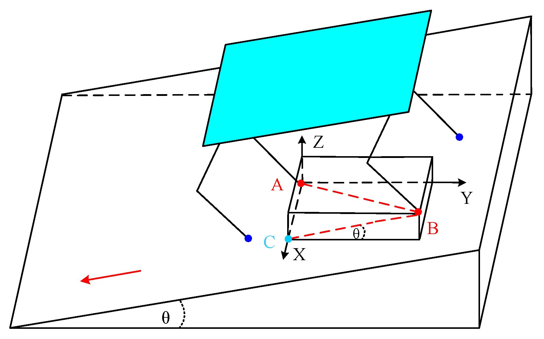
3.2. Slope Angle Estimation

To make the robot move on the slope better, it is very important for the robot to obtain the angle of the slope. In this work, a slope angle estimation method was designed, so that the quadruped robot can know the slope angle according to the coordinates of its foot ends without the aid of cameras. The estimation process is shown in Figure 6, where the red and blue dots indicate the position of the foot endpoints.

Connect A and B as diagonal lines to build a cuboid, as shown in Figure 6, let the coordinate of point A be ($x_A,y_A,z_A$), and the coordinate of point B is ($x_B,y_B,z_B$), select a point C ($x_C,y_C,z_C$) on the cuboid, where $x_C=x_B$, $y_C=y_A$, $z_C=z_A$, then the angle of the slope can be calculated as shown in Equation (5).

$$\begin{array}{cc}\hfill \theta & =arctan\frac{z_B-z_A}{y_B-y_A}.\hfill \end{array}$$

(5)

3.3. Deep Reinforcement Learning Algorithm

In this work, DRL is used to train the rhythm controller parameters to ensure the stable motion of the quadruped robot under different conditions. The DRL algorithm used in this work is the Soft Actor-Critic (SAC) [32,33].

The learning process of a quadruped robot can be regarded as the Markov decision process (MDP), which can be represented by a tuple ($S,A,P,r,\gamma$), where $S=\{s_1,s_2,\cdots ,s_T\}$ is the set of states, $A=\{a_1,a_2,\cdots ,a_T\}$ represents the set of actions, P is the state transition probability from the current state to the next state, r is the reward value for each step and $\gamma \in [0,1]$ represents the discount factor.

The usual mechanism for reinforcement learning is to find a strategy that maximizes cumulative reward; its expression is shown in Equation (6):

$$\begin{array}{c}\hfill {\pi }^{*}=arg\underset{\pi }{max}{\mathrm{E}}_{\pi }[\sum _{t}r(s_t,a_t)],\end{array}$$

(6)

where $\pi$ is the policy, ${\pi }^{*}$ is the optimal policy, E is the expected reward, t is time and $r(s_t,a_t)$ is the reward for choosing action $a_t$ in state $s_t$. The SAC algorithm, of course, also follows this rule, but the difference is that the SAC algorithm incorporates an entropy, which, in addition to maximizing the cumulative reward, makes the strategy more random; the expression is then shown in Equation (7):

$$\begin{array}{c}\hfill {\pi }^{*}=arg\underset{\pi }{max}{\mathrm{E}}_{\pi }[\sum _{t}r(s_t,a_t)+\alpha H(\pi (·|s_t))],\end{array}$$

(7)

where $H(\pi (·|s_t))$ is the entropy representing the degree of randomness of policy $\pi$ in state s and $\alpha$ is the regularization coefficient, which mainly controls the importance of the entropy.

In this work, the selected state space includes the position of the center of gravity of the robot, the motion speed of the robot on the X, Y and Z axes, the pitch angle, yaw angle, roll angle and the rotation angle of the eight joints during the robot’s movement; so, the state space can be expressed as $\{v_x,v_y,v_z,q_{pitch},q_{yaw},q_{roll},{\xi }_1,\cdots ,{\xi }_8\}$. From Equation (3), we know that the parameters of the rhythm controller include $A_k,A_h,T,{\phi }_0,{\phi }_1,{\phi }_2,{\phi }_3,{\phi }_4,{\phi }_5,{\phi }_6,{\phi }_7$. Since the gait used in this work is the trot gait, ${\phi }_0={\phi }_6=0,{\phi }_1={\phi }_7,{\phi }_2={\phi }_4=\pi ,{\phi }_3={\phi }_5$, the action space is $a=[A_k,A_h,T,{\phi }_1,{\phi }_3]$, which directly passes to the cosine rhythm controller to ensure that the controller works correctly, where $A_k\in [-0.5,0.5],A_h\in [-0.5,0.5],T\in (0,2],{\phi }_1\in [-2\pi ,2\pi ],{\phi }_3\in [-2\pi ,2\pi ]$.

In order to speed up the learning process, we set a penalty value, as long as the robot falls, where a punishment $r_p$ will be given, as shown in Equation (8), and the current round of training is then over.

$$\begin{array}{c}\hfill r_p=-100.\end{array}$$

(8)

At the same time, in order to encourage the robot to move, a reward $r_s$ is given to the robot for every step of movement, as shown in Equation (9):

$$\begin{array}{c}\hfill r_s=10.\end{array}$$

(9)

In order to encourage the robot to move forward, a forward reward is given to the robot. In this work, the forward direction of the robot is the Y direction (in the world coordinate system), so the forward reward function is

$$\begin{array}{c}\hfill r_y=w_1(y_{now}-y_{last}),\end{array}$$

(10)

where $y_{now}$ is the position of the robot in the Y direction at the current moment, $y_{last}$ is the position of the robot in the Y direction at the previous moment and $w_1$ is the forward reward function weight. Similarly, a reward function is given to the robot for the X direction, aiming to reduce the yaw of the robot; the reward function is shown in Equation (11):

$$\begin{array}{c}\hfill r_x=-w_2|x_{now}-x_{last}|,\end{array}$$

(11)

where $r_x$ is the reward for yawing, $x_{now}$ is the position of the robot in the X direction at the current moment and $x_{last}$ is the position of the robot in the X direction at the previous moment. In addition, in order to make the robot move more smoothly, the reward function is set for its pitch angle, roll angle and yaw angle, and the expression is shown in Equation (12):

$$\begin{array}{c}\hfill r_o=-w_3|q_{pitch}-\theta |-w_4|q_{yaw}|-w_5|q_{roll}|,\end{array}$$

(12)

where $r_o$ is the reward of orientation, $q_{pitch}$ is the pitch angle, $q_{yaw}$ is the yaw angle, $q_{roll}$ is the roll angle, $\theta$ is the angle of slope calculated by Equation (5) and $w_3$, $w_4$ and $w_5$ are the related weights. Therefore, the complete reward function r for the SAC is

$$\begin{array}{cc}\hfill r& =\alpha r_p+\beta (r_s+r_y+r_x+r_o)\hfill \\ \hfill & =-100\alpha +\beta (10+w_1(y_{now}-y_{last})-w_2|x_{now}-x_{last}|\hfill \\ \hfill & -w_3|q_{pitch}-\theta |-w_4|q_{yaw}|-w_5|q_{roll}|).\hfill \end{array}$$

(13)

When the robot falls down, $\alpha$ is 1 and $\beta$ is 0; otherwise, $\alpha$ is 0 and $\beta$ is 1. In addition, the selection of $w_1$,$w_2$,$w_3$,$w_4$ and $w_5$ must ensure that $r>0$ when $\alpha =0$ and $\beta =1$, so that the robot can learn to move forward. In this work, $w_1=150$, $w_2=100$, $w_3=30$, $w_4=40$ and $w_5=30$.

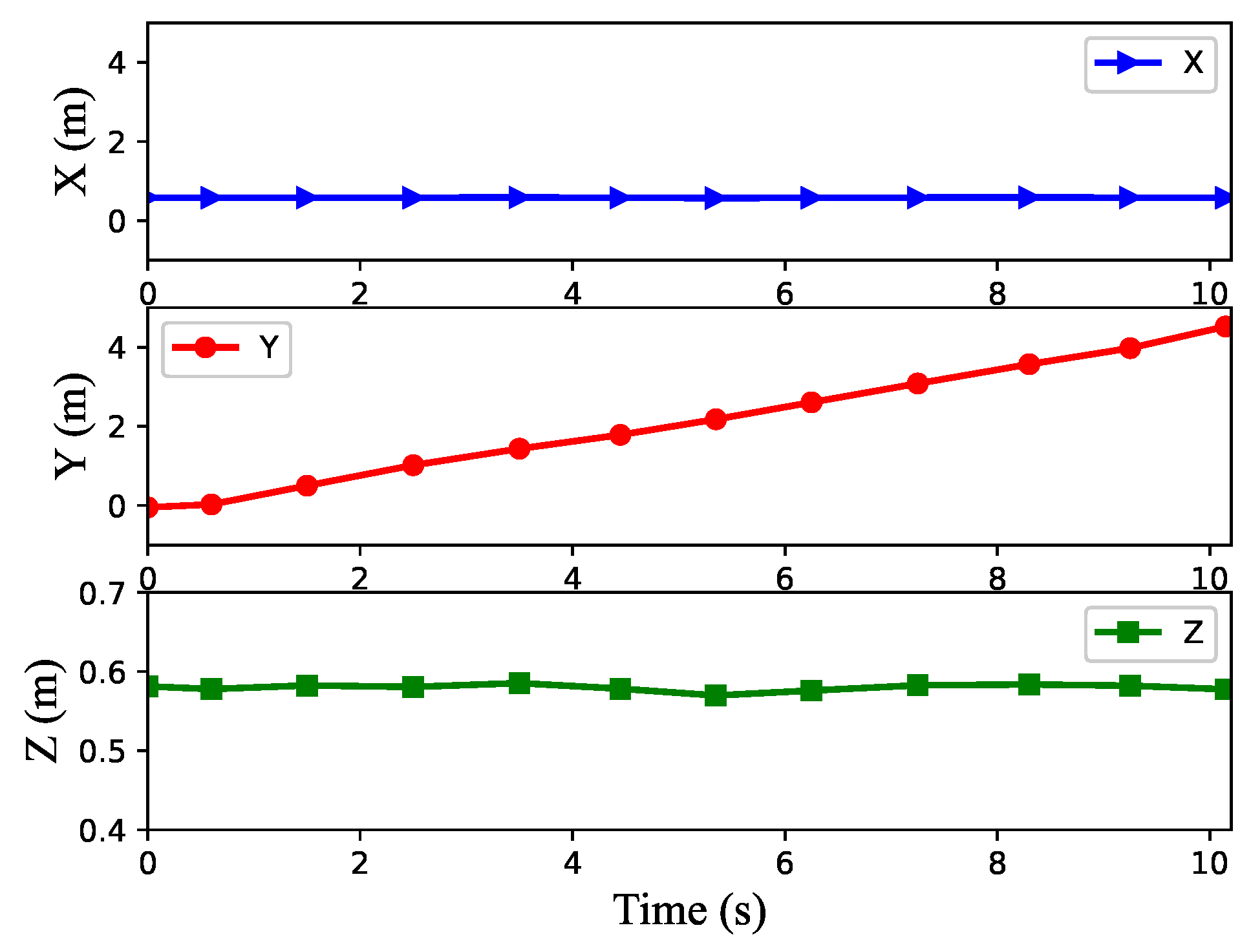
4. Simulation Results and Analysis

All the simulation experiments in this work are carried out in CoppeliaSim V4.0.0 [34], where the physics engine uses Bullet 2.83, the language used is Python, and the Python version used is Python 3.9

4.1. Flat Walking Task

In order to prove that the algorithm framework proposed in this work can complete the autonomous motion learning task of a quadruped robot, the robot was first made to carry out motion learning on a flat ground.

Figure 7 shows the reward value obtained by the quadruped robot trained in a virtual environment on flat ground. It can be seen clearly from the picture that the reward value increases rapidly from 0 to 1500 steps, meaning that the robot can quickly learn the movement, from the initial fall to the complete walk, which signifies that the robot can quickly learn the motor skills by using our proposed algorithm. By 9000 steps, the reward function value has exceeded 600, and the robot has learned good motion.

Figure 8 shows the position of the center of gravity when the robot moves on flat ground. The X direction represents the yaw direction, the Y direction represents the forward direction and the Z direction represents the direction of the body shaking up and down during the movement of the robot. It can be seen from the figure that the robot’s position in the Y direction is basically a straight line, which indicates that the robot presents uniform motion in the forward direction, especially during the period from 4.5 s to 9 s. From the Z direction, it can be seen that the robot would shake up and down in the process of lifting its legs and landing. Although there is a small amount of yaw in the X direction during movement, the maximum yaw is less than 0.12 m, and the robot is also corrected in real-time during the movement. Therefore, on the whole, the motion state of the robot is good, which proves that the algorithm proposed in this paper can achieve good movement of the robot.

Figure 9 shows the changes in the robot’s body posture in the process of movement. The solid line represents the learning result using the reward function r in this paper, while the dashed line represents the learning result using only $r_x$ and $r_y$ as $r_{xy}$. It can be seen from the figure that the yaw angle of the robot can be greatly reduced after learning with the reward function r compared with that of the reward function $r_{xy}$. This is because the addition of the reward function $r_o$ is equivalent to the constraint on the robot’s attitude, and the pitch angle and roll angle are not large, so the constraint effect is not very obvious.

It can be seen from Figure 8 and Figure 9 that the learning algorithm proposed in this paper can enable the robot to better complete the flat motion and basically achieve uniform straight motion on flat ground, and the pitch angle, yaw angle and roll angle all vary within a small range, with the maximum of 0.09, 0.10 and 0.09 radians, respectively.

4.2. Uphill and Downhill Task

In addition to flat movement, the quadruped robot can also carry out uphill and downhill movement in this work. Figure 10 shows a slope scene of 5°, which includes three sections: uphill, flat and downhill.

Figure 11 shows the uphill and downhill processes of the robot. Figure 11a,b show the process of the robot from the zero slope to the uphill slope; Figure 11b–d show the process of the robot going uphill; Figure 11d,e show the process of the robot from the uphill to zero slopes; Figure 11e–g show the process of the robot walking on a zero slope; Figure 11g,h represent the transition process of the robot from the zero slope to the downhill slope; Figure 11h,i show the process of the robot going downhill.

Figure 12 and Figure 13, respectively, show the position of the center of gravity and the attitude angle of the body when the robot is moving up and down hills in the scene in Figure 10. In Figure 12, the blue line represents the position change of the robot’s body center of gravity on the X axis; the red line represents its position change on the Y axis, which is also the robot’s direction of advance; the green line represents its change on the Z axis.

The blue line in Figure 13 represents the robot’s pitch angle, the red line represents the yaw angle, the green line represents the roll angle and the orange dashed line represents the expected pitch angle. By combining Figure 12 and Figure 13, we can learn that the robot starts to move uphill as shown in Figure 11b in about 4 s, arrives at the zero slope section in about 11.5 s as shown in Figure 11e and starts downhill as shown in Figure 11h in about 15.5 s. The speed of the robot on the uphill slope is smaller than that on the flat slope. It can also be seen that the robot’s pitch angle always follows the expected pitch angle during movement, that is to say, the robot could adjust its posture to adapt to the slope environment. In the process of movement, the maximum roll angle of the robot is no more than 0.1 radian, and it can be seen that the roll angle becomes larger when the robot starts to go uphill and downhill, while the rest of the rolling angle is small under stable conditions. Although the yaw angle of the robot in the uphill and downhill processes is larger than that in the flat movement, it can be seen from the X yaw direction that the robot movement does not produce a large yaw. Therefore, the algorithm proposed in this paper can help the robot learn better in climbing locomotion.

Figure 14 shows the output of the rhythm controller based on a cosine oscillator when the robot moved in the scene in Figure 10. We can see from the figure that the output of the rhythm controller during the robot movement has three modes, corresponding to the flat slope movement, uphill movement and downhill movement of the robot, respectively. From the figure, it is easy to see the difference in the output of the rhythm controller during the uphill and the flat slope; however, there is little difference in the output of the hip joint and some difference in the output of the knee joint in the process of flat and downhill motion. We can see from Figure 14 that our algorithm can output different patterns according to different environments to help the robot better cope with changes in the environment.

In addition, we also used the rhythm controller alone to control the robot for walking as shown in Figure 15. As can be seen from the figure, in the first six seconds under a set of parameters, the robot is able to move well on the flat ground. However, after six seconds, the robot encountered a slope of 5°; it could not climb the slope and fell down. Therefore, it can be concluded that a fixed set of rhythm controller parameters can only adapt the robot to one mode of motion, which also proves the power and superiority of our proposed algorithm.

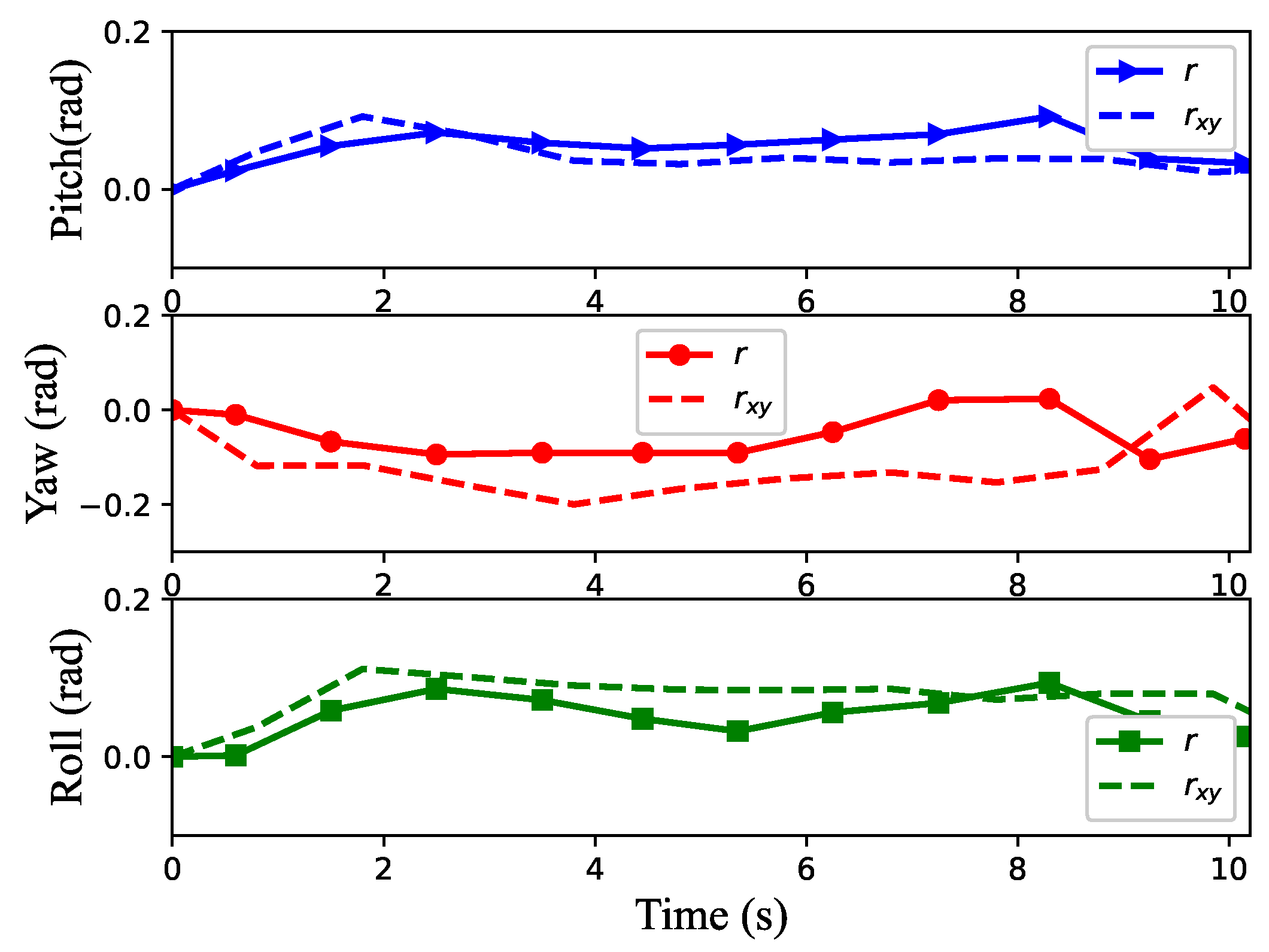
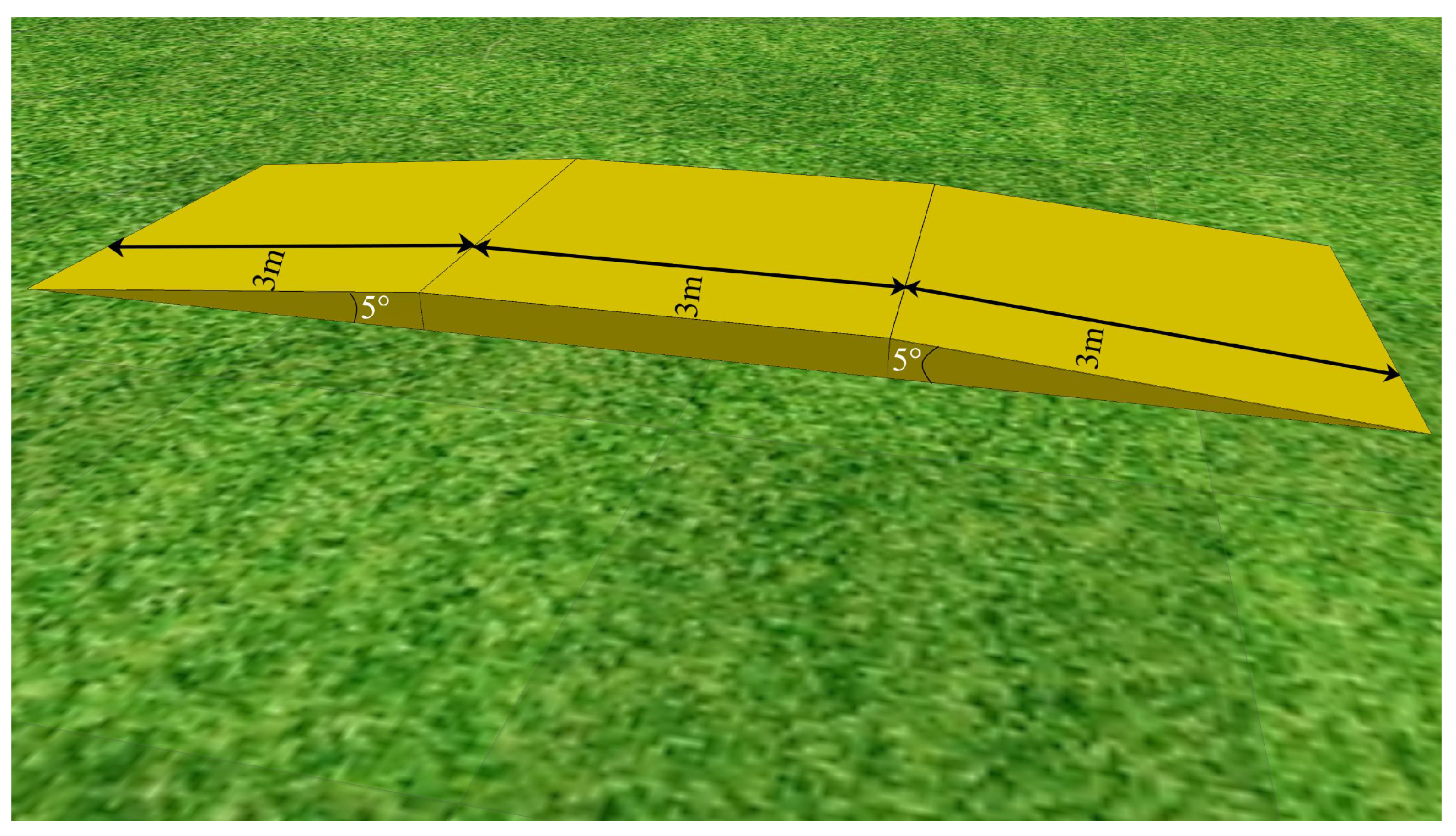
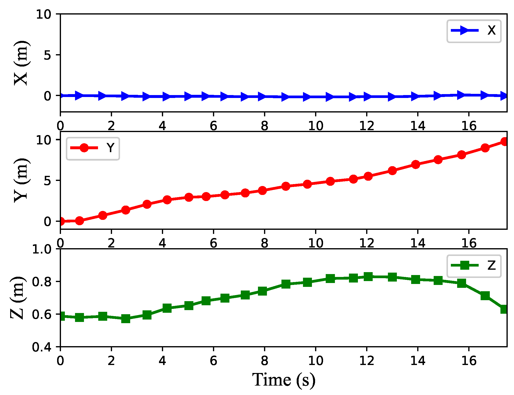
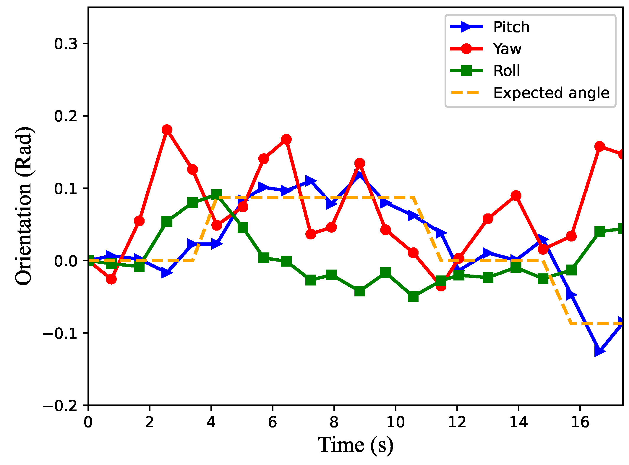
4.3. Unknown Scenario Task

In order to prove that the proposed algorithm can meet the requirements of the environmental adaptability of the quadruped robot, we also carried out an unknown scenario experiment. Under the condition that the robot was well trained with the 5° slope, the slope was changed to the one shown in Figure 16. The slope, called S-4, consisted of four sections, 5°, 0°, 9° and 0°, and each section is 1.4 m, 1.4 m, 1.2 m and 1.4 m, respectively.

Figure 17 and Figure 18 show the center of gravity position and body orientation of the robot, respectively. Combined with Figure 17 and Figure 18, it can be seen that the robot begins to climb the first slope in about 2.5 s, reaches the 0° slope in the second stage in about 5.6 s, climbs the 9° slope in the third stage in about 8.3 s, reaches the 0° slope in the fourth stage in about 15.1 s and, finally, stops on the slope. It also can be seen that the forward speed of the robot would decrease correspondingly when climbing the slope, and the higher the slope, the lower the speed. In addition, we can know from the figures that when the robot moves from one state to another state, the yaw angle of the robot will change greatly.

Figure 19 shows the output of the rhythm controller when the robot moves. We can see from the figure that except for the first step, the output state of the rhythm controller is basically the same from the second step to the fourth step. At this time, the robot was on flat ground or just started to climb the hill, and the controller outputted a pattern. At about 3.4 s, the robot was completely on the slope which was 5°, the controller outputted another pattern. Then, the robot entered the 0° slope, and the output of the controller was the same as that of the robot in the flat ground motion until the robot reached the 9° slope, where the rhythm controller outputted the third pattern.

Through this experiment, it can be proved that the algorithm proposed in this paper is robust and can make the robot cope with the change in the environment. Although the slope of 9° and the two uphill sections were never encountered before by the robot, it could still adapt to the changes well. In addition, we can see from Figure 19 that the rhythm controller can output different modes corresponding to different environments. Through the conversion between different modes, the robot can realize the adaptive movement of the environment.

5. Conclusions

In this work, a new kind of quadruped robot locomotion learning algorithm based on DRL and a rhythm controller was proposed to enable a robot to adapt to different kinds of environments. The rhythm controller is composed of eight cosine oscillators and, by configuring the phases of cosine oscillation, the complex coupling between the eight joints of the quadruped robot that needs to be considered in the CPG-based methods becomes simpler and easier to deal with here. In order to achieve the best rhythm controller parameters, the SAC algorithm was adopted. During the reward designing, in order to make sure that the quadruped robot can better adapt to the slope environment, a slope angle estimation method was proposed to obtain the slope angle based on the robot’s proprioceptive information, and the slope angle was added to the reward function. Compared to the DRL-only approach, the introduction of a newly designed rhythm controller can significantly improve the learning process. Experiments in different scenes show that the proposed algorithm can not only enable the robot to have good motor skills in the phases of flat, uphill and downhill, but also make it deal with an environment that it has never encountered before. The rhythm controller based on a cosine oscillator is simple and versatile, which can be applied to most kinds of legged robots, and provides great convenience for the migration to the physical robot. In this research, we only considered the robot’s forward movement. Next, we will improve the algorithm in the future to make the robot able to adjust its gait and adaptively track different trajectories.

References

1. Chang, X.; Ma, H.; An, H. Quadruped robot control through model predictive control with pd compensator. Int. J. Control. Autom. Syst. 2021, 19, 3776–3784. [Google Scholar] [CrossRef]
2. Kim, J.; Ba, D.X.; Yeom, H.; Bae, J. Gait optimization of a quadruped robot using evolutionary computation. J. Bionic Eng. 2021, 18, 306–318. [Google Scholar] [CrossRef]
3. Sakakibara, Y.; Kan, K.; Hosoda, Y.; Hattori, M.; Fujie, M. Foot trajectory for a quadruped walking machine. In Proceedings of the IEEE International Workshop on Intelligent Robots and Systems, Towards a New Frontier of Applications, Ibaraki, Japan, 3–6 July 1990; pp. 315–322. [Google Scholar]
4. Sun, L.; Meng, M.Q.H.; Chen, W.; Liang, H.; Mei, T. Design of quadruped robot based neural network. In Proceedings of the Advances in Neural Networks—ISNN 2007: 4th International Symposium on Neural Networks, ISNN 2007, Nanjing, China, 3–7 June 2007; Proceedings, Part I 4. Springer: Berlin/Heidelberg, Germany, 2007; pp. 843–851. [Google Scholar]
5. Li, X.; Zhang, X.; Niu, J.; Li, C. A stable walking strategy of quadruped robot based on zmp in trotting gait. In Proceedings of the 2022 IEEE International Conference on Mechatronics and Automation (ICMA), Guangxi, China, 7–10 August 2022; IEEE: New York, NY, USA, 2022; pp. 858–863. [Google Scholar]
6. Ding, Y.; Pandala, A.; Park, H.W. Real-time model predictive control for versatile dynamic motions in quadrupedal robots. In Proceedings of the 2019 International Conference on Robotics and Automation (ICRA), Montreal, QC, Canada, 20–24 May 2019; IEEE: New York, NY, USA, 2019; pp. 8484–8490. [Google Scholar]
7. Zhang, G.; Rong, X.; Hui, C.; Li, Y.; Li, B. Torso motion control and toe trajectory generation of a trotting quadruped robot based on virtual model control. Adv. Robot. 2016, 30, 284–297. [Google Scholar] [CrossRef]
8. Zhang, S.; Gao, J.; Duan, X.; Li, H.; Yu, Z.; Chen, X.; Li, J.; Liu, H.; Li, X.; Liu, Y.; et al. Trot pattern generation for quadruped robot based on the zmp stability margin. In Proceedings of the In 2013 ICME International Conference on Complex Medical Engineering, Beijing, China, 25–28 May 2013; IEEE: New York, NY, USA, 2013; pp. 608–613. [Google Scholar]
9. Du, Y.; Gao, S.; Huiping Li, H.; Cui, D. Mpc-based tilting and forward motion control of quadruped robots. In Proceedings of the 2022 5th International Symposium on Autonomous Systems (ISAS), Hangzhou, China, 8–10 April 2022; IEEE: New York, NY, USA, 2022; pp. 1–6. [Google Scholar]
10. Harris-Warrick, R.M. Neuromodulation and flexibility in central pattern generator networks. Curr. Opin. Neurobiol. 2011, 21, 685–692. [Google Scholar] [CrossRef] [PubMed]
11. Wang, T.; Guo, W.; Li, M.; Zha, F.; Sun, L. Cpg control for biped hopping robot in unpredictable environment. J. Bionic Eng. 2012, 9, 29–38. [Google Scholar] [CrossRef]
12. Matsuoka, K. Sustained oscillations generated by mutually inhibiting neurons with adaptation. Biol. Cybern. 1985, 52, 367–376. [Google Scholar] [CrossRef] [PubMed]
13. Kimura, H.; Akiyama, S.; Sakurama, K. Realization of dynamic walking and running of the quadruped using neural oscillator. Auton. Robot. 1999, 7, 247–258. [Google Scholar] [CrossRef]
14. Xiao, W.; Wang, W. Hopf oscillator-based gait transition for a quadruped robot. In Proceedings of the 2014 IEEE International Conference on Robotics and Biomimetics (ROBIO 2014), Bali, Indonesia, 5–10 December 2014; IEEE: New York, NY, USA, 2014; pp. 2074–2079. [Google Scholar]
15. Xie, J.; Ma, H.; Wei, Q.; An, H.; Su, B. Adaptive walking on slope of quadruped robot based on cpg. In Proceedings of the 2019 2nd World Conference on Mechanical Engineering and Intelligent Manufacturing (WCMEIM), Shanghai, China, 22–24 November 2019; IEEE: New York, NY, USA, 2019; pp. 487–493. [Google Scholar]
16. Zhang, J.; Gao, F.; Han, X.; Chen, X.; Han, X. Trot gait design and cpg method for a quadruped robot. J. Bionic Eng. 2014, 11, 18–25. [Google Scholar] [CrossRef]
17. Zhang, Y.; Wang, H.; Ding, Y.; Hou, B. Adaptive walking control for a quadruped robot on irregular terrain using the complexvalued cpg network. Symmetry 2021, 13, 2090. [Google Scholar] [CrossRef]
18. Tan, J.; Zhang, T.; Coumans, E.; Iscen, A.; Bai, Y.; Hafner, D.; Bohez, S.; Vanhoucke, V. Sim-to-real: Learning agile locomotion for quadruped robots. arXiv 2018, arXiv:1804.10332. [Google Scholar]
19. Tsounis, V.; Alge, M.; Lee, J.; Farshidian, F.; Hutter, M. Deepgait: Planning and control of quadrupedal gaits using deep reinforcement learning. IEEE Robot. Autom. Lett. 2020, 5, 3699–3706. [Google Scholar] [CrossRef]
20. Bogdanovic, M.; Khadiv, M.; Righetti, L. Model-free reinforcement learning for robust locomotion using trajectory optimization for exploration. arXiv 2021, arXiv:2107.06629v1. [Google Scholar]
21. Hu, B.; Shao, S.; Cao, Z.; Xiao, Q.; Li, Q.; Ma, C. Learning a faster locomotion gait for a quadruped robot with model-free deep reinforcement learning. In Proceedings of the 2019 IEEE International Conference on Robotics and Biomimetics (ROBIO), Dali, China, 6–8 December 2019; IEEE: New York, NY, USA, 2019; pp. 1097–1102. [Google Scholar]
22. Haarnoja, T.; Ha, S.; Zhou, A.; Tan, J.; Tucker, G.; Levine, S. Learning to walk via deep reinforcement learning. arXiv 2018, arXiv:1812.11103. [Google Scholar]
23. Zhu, X.; Wang, M.; Ruan, X.; Chen, L.; Ji, T.; Liu, X. Adaptive motion skill learning of quadruped robot on slopes based on augmented random search algorithm. Electronics 2022, 11, 842. [Google Scholar] [CrossRef]
24. Lee, H.; Shen, Y.; Yu, C.H.; Singh, G.; Ng, A.Y. Quadruped robot obstacle negotiation via reinforcement learning. In Proceedings of the 2006 IEEE International Conference on Robotics and Automation, 2006, ICRA 2006, Orlando, FL, USA, 15–19 May 2006; IEEE: New York, NY, USA, 2006; pp. 3003–3010. [Google Scholar]
25. Bellegarda, G.; Ijspeert, A. Cpg-rl: Learning central pattern generators for quadruped locomotion. IEEE Robot. Autom. Lett. 2022, 7, 12547–12554. [Google Scholar] [CrossRef]
26. Ijspeert, A.J.; Crespi, A.; Ryczko, D.; Cabelguen, J.M. From swimming to walking with a salamander robot driven by a spinal cord model. Science 2007, 315, 1416–1420. [Google Scholar] [CrossRef] [PubMed]
27. Rudin, N.; Kolvenbach, H.; Tsounis, V.; Hutter, M. Cat-like jumping and landing of legged robots in low gravity using deep reinforcement learning. IEEE Trans. Robot. 2021, 38, 317–328. [Google Scholar] [CrossRef]
28. Lee, C.; An, D. Reinforcement learning and neural network-based artificial intelligence control algorithm for self-balancing quadruped robot. J. Mech. Sci. Technol. 2021, 35, 307–322. [Google Scholar] [CrossRef]
29. Liu, K.; Zhao, J.; Wang, M.; Wang, Z.; Liang, W. Gait planning and simulation analysis of quadruped robot. In Proceedings of the 2021 IEEE 5th Information Technology, Networking, Electronic andAutomation Control Conference (ITNEC), Xi’an, China, 15–17 October 2021; IEEE: New York, NY, USA, 2021; Volume 5, pp. 274–278. [Google Scholar]
30. Liu, Z.; Ding, X. Gait generation of quadruped robot based on cosine oscillator. Comput. Simul. 2013, 30, 365–369. [Google Scholar]
31. Zhang, X.L. Biological-Inspired Rhythmic Motion and Environmental Adaptability for Quadruped Robot. Ph.D. Thesis, Tsinghua University, Beijing, China, 2004. [Google Scholar]
32. Haarnoja, T.; Zhou, A.; Abbeel, P.; Levine, S. Soft actor-critic: Off-policy maximum entropy deep reinforcement learning with a stochastic actor. In Proceedings of the International Conference on Machine Learning, Stockholm, Sweden, 10–15 July 2018; pp. 1861–1870. [Google Scholar]
33. Haarnoja, T.; Zhou, A.; Hartikainen, K.; Tucker, G.; Ha, S.; Tan, J.; Kumar, V.; Zhu, H.; Gupta, A.; Abbeel, P.; et al. Soft actor-critic algorithms and applications. arXiv 2018, arXiv:1812.05905. [Google Scholar]
34. CoppeliaSim. Available online: https://www.coppeliarobotics.com (accessed on 19 March 2022).
Figure 1. The quadruped robot, where LF represents the left-front leg, RF represents the right-front leg, LB represents the left-back leg, and RB represents the right-back leg. The direction of the red arrow is straight ahead.
Applsci 13 11045 g001
Figure 2. Trot gait pattern. The black squares indicate that the robot’s legs are in the swing phase, and the white squares indicate that the robot’s legs are in the support phase.
Applsci 13 11045 g002
Figure 3. Quadruped robot adaptive locomotion learning algorithm architecture.The blue line output by the control unit represents the hip signal, and the red line represents the knee signal.
Applsci 13 11045 g003
Figure 4. Output of the single-legged control unit.
Applsci 13 11045 g004
Figure 5. Four-legged rhythm controller structure, where the hip joints are represented by h, the knee joints are represented by k, B represents the body, and the dashed lines represent the coupling between two joints, represented by φ i j .
Applsci 13 11045 g005
Figure 6. The robot is on the slope. The red and blue dots indicate the position of the foot endpoints.
Applsci 13 11045 g006
Figure 7. Reward.
Applsci 13 11045 g007
Figure 8. Curves of the robot’s center of gravity position during walking on flat ground.
Applsci 13 11045 g008
Figure 9. Attitude curves of the robot during walking.
Applsci 13 11045 g009
Figure 10. Slope of 5°. The yellow slope has three sections, which are 5° uphill, 0° slope and 5° downhill, and each section is 3m as shown in the black line segment.
Applsci 13 11045 g010
Figure 11. Robot uphill and downhill processes.
Applsci 13 11045 g011
Figure 12. The robot’s center of gravity position during movement in the scene in Figure 10.
Applsci 13 11045 g012
Figure 13. The orientation of the robot during movement in the scene in Figure 10.
Applsci 13 11045 g013
Figure 14. The output of the cosine rhythm controller during movement in the scene in Figure 10.
Applsci 13 11045 g014
Figure 15. The center of gravity curve of the robot when using fixed cosine rhythm controller parameters.
Applsci 13 11045 g015
Figure 16. The slope called S-4, which has 4 sections. The first section is 5° uphill slope which is 1.4 m, as shown by the black line segment with arrows, the second section is a 0° slope which is 1.4 m, the third section is a 9° uphill slope which is 1.2 m, and the fourth section is a 0° slope which is 1.4 m.
Applsci 13 11045 g016
Figure 17. The robot’s center of gravity position when climbing S-4.
Applsci 13 11045 g017
Figure 18. The orientation of the robot when climbing S-4.
Applsci 13 11045 g018
Figure 19. The output of the cosine rhythm controller when the robot climbed S-4.
Applsci 13 11045 g019
Disclaimer/Publisher’s Note: The statements, opinions and data contained in all publications are solely those of the individual author(s) and contributor(s) and not of MDPI and/or the editor(s). MDPI and/or the editor(s) disclaim responsibility for any injury to people or property resulting from any ideas, methods, instructions or products referred to in the content.