A Novel Zeroing Neural Network Control Scheme for Tracked Mobile Robot Based on an Extended State Observer

Abstract

A novel zeroing neural network control scheme based on an extended state observer is proposed for the trajectory tracking of a tracked mobile robot which is subject to unknown external disturbances and uncertainties. To estimate unknown lumped disturbances and unmeasured velocities, a third-order fixed-time extended state observer is proposed, and the observation errors converge to zero in fixed time. Based on the estimated values, the zeroing neural network controller is designed for a tracked mobile robot to track an eight shape. The stability of the system is analyzed based on Lyapunov theory. Simulation results are illustrated to show the effectiveness of the proposed control scheme.

1. Introduction

Tracked mobile robots (TMRs) have a wide range of applications in civil, industrial and military fields. However, TMRs are typical nonlinear systems, and it is difficult to perform high-precision trajectory-tracking control [1,2]. To enhance the control performance of mobile robots, a feasible solution with excellent convergence performance and robustness is imperative in practice. Numerous control methods to address this tracking issue have been reported, including sliding mode control (SMC) [3,4], backstepping control [5], model predictive control [6], adaptive control [7,8], etc. In [9], a control method was proposed for a skid-steering mobile robot based on the kinematic control concept and the input–output linearization approach. Chen et al. derived the error dynamics of the path using the combination of the kinematic model of the robot and designed a horizontal steering control law for the path following of the mobile robot [10]. The authors of [11] developed an integer-order prescribed-time controller for a four-wheel independently driven skid-steering mobile robot while considering various disturbances.

In recent decades, a new recurrent network, called zeroing neural network (ZNN), has attracted the interest of scholars with its potential for parallel computing and nonlinear processing [12]. The ZNN and its evolved model have been reported to solve robot manipulator quadratic programming [13,14] and trajectory tracking [15,16]. Chen et al. proposed a novel supertwisting ZNN to address the tracking control of a robot manipulator [17] which combines SMC and ZNN successfully. Ma et al. developed a ZNN for a bound-constrained omnidirectional mobile robot manipulator by introducing a time-varying non-negative vector [18].

The successful application in robot manipulators motivates us to further explore ZNN application in mobile robots [19], which is a potential field. In [20], a multi-constrained ZNN with the exponential-convergence property was demonstrated by utilizing the time-derivative information, and it was applied to a mobile robot with both performance index optimization and multiple physical-limit constraints. A robust fast-convergence zeroing neural network was proposed in [21] to implement trajectory-tracking application in a noisy environment. A ZNN activated through finite-time-convergence activation was employed for TMR kinematics to track the desired trajectory [22]. The above-mentioned papers about mobile robot trajectory tracking are based on the perspective of kinematic models, which assumes perfect speed tracking [23]. As for an actual situation, the physical parameters of mobile robots, such as mass, inertia, have an impact on system control. Therefore, it is necessary to extend the study of ZNNs to the dynamic level of mobile robots.

Moreover, TMRs always work in harsh environments. These papers assume that all the states of the mobile robot are known and accurate and so are the disturbances. However, if the velocity cannot be measured due to sensor faults, the ZNN models proposed above are not viable. Therefore, it is necessary to design a state observer in the ZNN framework to improve the performance of the system. A key feature of an observer is the convergence rate. In a specific situation, there is a great need for rapid convergence of observers to complete the state reconstruction [24]. And some fast-convergence observers have been developed [25,26,27]. Fan et al. proposed a fast–finite-time-convergence observer formation control scheme for nonholonomic mobile robots [28]. In [29], Roger presented an observer-based PID for the trajectory-tracking control of wheeled mobile robots with kinematic interferences.

However, the upper bound of the settling time is dependent on the initial states for finite-time-convergence observers. In view of this, fixed-time-convergence state observers are explored, which guarantees that the settling time of observer errors is irrelevant with respect to the initial conditions. Zhang et al. demonstrated a fixed-time extended state observer (FTESO) for marine surface vessel trajectory tracking [30]. In [31], fixed-time neuroadaptive practical tracking control based on an extended state observer was proposed for a quadrotor unmanned aerial vehicle with external disturbances and time-varying parameters.

It can be concluded that ZNNs have not been applied to mobile robot dynamic control, since its application faces unsolved challenges. One is that unmeasured velocities encountered in practice lead to failure in building a ZNN control framework. The other is how to achieve noise suppression and fast convergence simultaneously. To address the above challenges, a novel activation function with fixed-time convergence and noise suppression is introduced. Then, an FTESO is employed to estimate the unmeasured velocities and quickly construct a ZNN model. Finally, a fixed-time-convergence ZNN model (FXZNN) based on the FTESO is proposed in this paper to achieve the fast tracking of the desired velocity, as well the trajectory, even with unmeasured velocities and external disturbances. To the best of our knowledge, this is the first ZNN control framework based on an observer for TMR tracking control. The main contributions of this paper are as follows:

(1)

An FTESO is designed to estimate the TMR’s unmeasured velocity as well the lumped disturbances in the system.

(2)

An FTESO-based FXZNN model is proposed to improve the desired velocities, convergence speed and tracking control performance of the system with the novel activation function adopted.

(3)

The velocity estimation error between the estimation and the actual values is adopted for constructing the error function of the proposed ZNN model.

This paper is organized as follows: Section 2 presents the modified TMR kinematic and dynamic model. Section 3 describes the tracking problem of the TMR. In Section 3, we demonstrate the design of the FXZNN model based on an FTESO for the TMR and present the corresponding stability analysis of the model using Lyapunov theory. Simulation results of the proposed model are given in Section 4, followed by the conclusion in Section 5.

2. Problem Formulation

In a global $XOY$ coordinate system, the schematic diagram of the motion of a TMR is presented in Figure 1. Some notations mentioned in Figure 1 are listed in Table 1. Considering the skidding case, the TMR satisfies the following constraint [32]:

$$A\left(q\right)\dot{q}=\xi ,$$

(1)

where $q={\left[\begin{array}{ccc}x& y& \theta \end{array}\right]}^T$ denotes the position and orientation of the TMR, $A\left(q\right)=\left[\begin{array}{ccc}-sin\left(\theta \right)& -cos\left(\theta \right)& 0\end{array}\right]$ is a vector of nonholonomic constraints, $\xi$ is the lateral skidding velocity.

Table 1. Notations in Figure 1.

Notation	Meaning
$(X,O,Y)$	The global coordinate system
$(X_1,O_1,Y_1)$	The coordinate system attached to the TMR
$q(x,y,\theta )$	The actual position
$q(x_d,y_d,{\theta }_d)$	The desired position
$(x_e,y_e,{\theta }_e)$	The tracking error
$v_c$	The linear velocity generated by the kinematic controller
${\omega }_c$	The angular velocity generated by the kinematic controller

The TMR kinematic model subject to skidding disturbance can be expressed as

$$\dot{q}=J\left(q\right)z+\phi (q,\xi ),$$

(2)

where $\phi (q,\xi )={\left[\begin{array}{cc}{\rho }_1& {\rho }_2\end{array}\right]}^T$ is the vector of the disturbance caused by the skidding velocity, with ${\rho }_1=-\xi sin\left(\theta \right)$, ${\rho }_1=-\xi sin\left(\theta \right)$, $J\left(q\right)={\left[\begin{array}{ccc}cos\left(\theta \right)& sin\left(\theta \right)& 0\\ 0& 0& 1\end{array}\right]}^T$, $z={\left[\begin{array}{cc}v& \omega \end{array}\right]}^T$, with $v,\omega$ denoting the linear and the angular velocities, respectively.

Assumption 1.

The perturbation $\phi (q,\xi )$ is bounded because of $∥{\left[-sin\left(\theta \right),cos\left(\theta \right)\right]}^T∥=1$, where $∥·∥$ is the Euclidean norm of the vector. Its first derivatives is also bounded.

Figure 1. Schematic diagram of TMR motion.

The dynamic model of the TMR can be described by the following equation:

$$M\left(q\right)\ddot{q}+C(q,\dot{q})\dot{q}+G\left(q\right)=B\left(q\right)\tau +A^T\left(q\right)\kappa +d.$$

(3)

where $M\left(q\right)$ denotes a symmetric and positive defined inertia matrix; $C\left(q,\dot{q}\right)$ is a Coriolis–centripetal matrix; $G\left(q\right)$ represents a gravity vector; $B\left(q\right)$ is an input transformation matrix; $\tau ={\left[\begin{array}{cc}{\tau }_l& {\tau }_r\end{array}\right]}^T$ are the control inputs, with ${\tau }_l$ and ${\tau }_r$ denoting torques of the left and right sides, respectively; $\kappa =-m(\dot{x}cos\left(\theta \right)+\dot{y}sin\left(\theta \right))\dot{\theta }$ represents the vector of the Lagrange multiplier; d is the bounded external environmental disturbance.

The matrices $M\left(q\right)$, $B\left(q\right)$ above are defined as follows:

$$M\left(q\right)=\left[\begin{array}{ccc}m& 0& 0\\ 0& m& 0\\ 0& 0& I\end{array}\right],B\left(q\right)=\frac{1}{r}\left[\begin{array}{cc}cos\left(\theta \right)& sin\left(\theta \right)\\ sin\left(\theta \right)& sin\left(\theta \right)\\ b& -b\end{array}\right],$$

where m is the overall mass of the TMR, I is the inertia, r represents the radius of the wheel and h represents half of the distance between the track wheels.

The differential form of (2) is shown below:

$$\ddot{q}=\dot{J}\left(q\right)z+J\left(q\right)\dot{z}+\dot{\phi }(q,\xi ).$$

(4)

Notice that $A\left(q\right)J\left(q\right)=0$, and it is assumed that the distance between the center of the TMR form and its center of mass is zero, so the effect of $C(q,\dot{q})$ can be eliminated from (3). By multiplying both sides by $J^T\left(q\right)$ simultaneously, with (4) being substituted into Equation (3), one can obtain

$$\overline{M}\dot{z}=\overline{B}\tau +\overline{d},$$

(5)

where $\overline{M}=J^{T}MJ$, $\overline{B}=J^{T}B$, $\overline{d}=J^T[d-M\dot{\phi }-M\dot{J}z-G]={\left[\begin{array}{cc}{\rho }_3& {\rho }_4\end{array}\right]}^T$. Evidently, the term $\overline{d}$ contains the information of the unmeasured velocities and other external disturbances. Therefore, it is considered to be the lumped disturbance in the model.

Assumption 2.

According to [33], the lumped disturbance ($\overline{d}$) satisfies the inequality $∥\overline{d}∥<D$, where D is a bounded constant.

Further, (5) can be reformulated as

$$\dot{z}={\overline{M}}^{-1}\overline{B}(\tau +\overline{d}),$$

(6)

The objective of this brief is that the FXZNN control scheme based on an FTESO is developed for a TMR to suppress the influence of the lumped disturbance that exists in the system, deal with the unmeasured velocities and improve trajectory-tracking performance.

3. Main Results

3.1. Preliminaries and Notations

Consider the following nonlinear system:

$$\dot{x}\left(t\right)=f(t,x),x\left(0\right)=0,f\left(x\left(0\right)\right)=0,$$

(7)

where $x\left(t\right)\in R^n$, $f(t,x)$ denotes the smooth nonlinear function and it is assumed that the origin is the equilibrium point of system (7).

Definition 1

([25]). Let us assume that system (7) is globally asymptotically stable. If there exists a finite convergence time T for all $t⩾T$ satisfying $x\left(t\right)\equiv 0$, then system (7) is globally finite-time-stable.

Definition 2

([34]). System (7) is globally finite-time-stable. For $\forall x_0\in R^n$, there exists $T⩽T_s$, $T_s\in R$, denoting a bounded positive value; then, system (7) is globally fixed-time-stable.

Lemma 1

([35]). If a continuous radial bounded function $V\left(x\right)$: $R^n\to R_{+}\cup \left\{0\right\}$ satisfies $\dot{V}\left(x\right)⩽-{\left(j_1{V}_1^a\left(x\right)-j_2{V}_2^a\left(x\right)\right)}^{a_3}+\vartheta$, with $V\left(x\right)=0\iff x=0$, where $\vartheta \in (0,+\infty )$, $\left\{a_1,a_2,a_3,j_1,j_2\right\}>0$, $a_1{a}_3<1,a_2{a}_3>1$, then the system is globally stable and converges to the balance point in fixed time T. Its convergence time T satisfies the inequality

$$T⩽T_{max}:=\frac{1}{j_1^k\iota (1-a_1{a}_3)}+\frac{1}{j_2^k\iota (a_2{a}_3-1)},$$

(8)

where ι is a positive constant, with $0<\iota <1$.

Some notations used in the paper are shown below.

(1)

Considering a given vector, ${∥·∥}_2$ is defined as the Euclidean 2-norm. $\left|·\right|$ represents the absolute value of a scalar. ${\lambda }_{min}\left\{·\right\}$ and ${\lambda }_{max}\left\{·\right\}$ denote the minimum and maximum eigenvalue values of a matrix $\left\{·\right\}$, respectively.

(2)

We denote $x={\left[x_1,x_2,...,x_n\right]}^T$ and $si{g}^{\alpha }\left(x\right)={\left[si{g}^{\alpha }\left(x_1\right),si{g}^{\alpha }\left(x_2\right),...,si{g}^{\alpha }\left(x_n\right)\right]}^T$, where $si{g}^{\alpha }\left(x_i\right)=sgn\left(x_i\right){\left|x_i\right|}^{\alpha }(i=1,2,...,n)$, where $sgn(·)$ is the signum function, $x_i\in R,\alpha \in (0,1)$, respectively.

3.2. FTESO Design

In this subsection, we explore an FTESO to estimate unmeasured velocities v, $\omega$ and lumped disturbance $\overline{d}$. To design the observer, the model of the TMR in (6) is converted into the following form:

$$\left\{\begin{array}{c}\dot{x}=vcos\left(\theta \right)-{\rho }_1,\\ \dot{y}=vsin\left(\theta \right)+{\rho }_2,\\ \dot{\theta }=\omega .\hfill \end{array}\right.$$

(9)

$$\left\{\begin{array}{c}m\dot{v}=\frac{1}{r}{\tau }_v+{\rho }_3,\hfill \\ \overline{I}\dot{\omega }=\frac{R}{r}{\tau }_{\omega }+{\rho }_4.\hfill \end{array}\right.$$

(10)

where ${\tau }_v={\tau }_l+{\tau }_r,{\tau }_{\omega }={\tau }_l-{\tau }_r$. Further, (9) and (10) can be converted into two cascade subsystems:

$$\left\{\begin{array}{c}\dot{x}=vcos\left(\theta \right)-{\rho }_1,\hfill \\ \dot{y}=vsin\left(\theta \right)+{\rho }_2,\hfill \\ \dot{v}=\frac{1}{mr}{\tau }_v+\frac{1}{m}{\rho }_3.\hfill \end{array}\right.$$

(11)

$$\left\{\begin{array}{c}\dot{\theta }=\omega ,\hfill \\ \dot{\omega }=\frac{R}{\overline{I}r}{\tau }_{\omega }+\frac{1}{\overline{I}}{\rho }_4.\hfill \end{array}\right.$$

(12)

Based on Assumption 2, the following FTESO is designed to obtain an accurate estimation of the unmeasured angular velocity $\omega$ and perturbation ${\rho }_4$ in the equations.

$$\left\{\begin{array}{c}\dot{\widehat{\theta }}=\widehat{\omega }+{\mu }_{1}si{g}^{{\alpha }_1}(\theta -\widehat{\theta })+{\epsilon }_{1}si{g}^{{\beta }_1}(\theta -\widehat{\theta }),\hfill \\ \dot{\widehat{\omega }}=\frac{R}{\overline{I}r}{\tau }_{\omega }+\frac{1}{\overline{I}}{\widehat{\rho }}_4+{\mu }_{2}si{g}^{{\alpha }_2}(\theta -\widehat{\theta })+{\epsilon }_{2}si{g}^{{\beta }_2}(\theta -\widehat{\theta }),\hfill \\ {\dot{\widehat{\rho }}}_4={\mu }_{3}si{g}^{{\alpha }_3}(\theta -\widehat{\theta })+{\epsilon }_{3}si{g}^{{\beta }_3}(\theta -\widehat{\theta })+{\rm Y}tanh(\theta -\widehat{\theta }).\hfill \end{array}\right.$$

(13)

where $\widehat{\theta }$, $\widehat{\omega }$, ${\widehat{\rho }}_4$ are the observation values of $\theta$, $\omega$, ${\rho }_4$; the parameters ${\alpha }_i=i\overline{\alpha }-(i-1)$, ${\beta }_i=i\overline{\beta }-(i-1)$, $i=1,2,3$, $\overline{\alpha }\in (1-m_1,1)$, $\overline{\beta }\in (1,1+m_2)$; ${\rm Y}>D$; $m_1$ and $m_2$ are two positive constants. The FTESO (13) gains are assigned to ensure that the matrices A, $A_1$ are Hurwitz, with $A=\left[\begin{array}{ccc}-{\mu }_1& 1& 0\\ -{\mu }_2& 0& 1\\ -{\mu }_3& 0& 0\end{array}\right]$, $A_1=\left[\begin{array}{ccc}-{\epsilon }_1& 1& 0\\ -{\epsilon }_2& 0& 1\\ -{\epsilon }_3& 0& 0\end{array}\right]$.

Theorem 1.

The states θ, ω and the disturbance ${\rho }_4$ can be estimated using FTESO (13) in fixed time $T_1$, with $T_1$ being denoted as

$$T_1⩽\frac{{\lambda }_{max}^{\rho }\left(P\right)}{r_2\rho }+\frac{1}{r_2\sigma {\varpi }^{\sigma }},$$

(14)

where $\rho =1-\overline{\alpha },\sigma =\overline{\beta }-1$, $r_1=\frac{{\lambda }_{min}\left(Q\right)}{{\lambda }_{max}\left(P\right)},r_2=\frac{{\lambda }_{min}\left(Q_1\right)}{{\lambda }_{max}\left(P_1\right)}$, $\varpi ⩽{\lambda }_{min}\left(P_1\right)$ is a positive constant. The symmetric positive matrices $P,Q,P_1,Q_1$ satisfy the function

$$\left\{\begin{array}{c}PA+A^{T}P=-Q,\hfill \\ P_1{A}_1+A_1^T{P}_1=-Q_1.\hfill \end{array}\right.$$

(15)

Proof. 

The estimation error of the observer is defined as

$$\left\{\begin{array}{c}\tilde{\theta }=\theta -\widehat{\theta },\hfill \\ \tilde{\omega }=\omega -\widehat{\omega },\hfill \\ {\tilde{\rho }}_4={\rho }_4-{\widehat{\rho }}_4.\hfill \end{array}\right.$$

(16)

The derivative of (16) is given as

$$\left\{\begin{array}{c}\dot{\tilde{\theta }}=\tilde{\omega }-{\mu }_{1}si{g}^{{\alpha }_1}(\theta -\widehat{\theta })-{\epsilon }_{1}si{g}^{{\beta }_1}(\theta -\widehat{\theta }),\hfill \\ \dot{\tilde{\omega }}=\frac{1}{\overline{I}}{\tilde{\rho }}_4-{\mu }_2(si{g}^{{\alpha }_2}(\theta -\widehat{\theta })-{\epsilon }_{2}si{g}^{{\beta }_2}(\theta -\widehat{\theta }),\hfill \\ {\dot{\tilde{\rho }}}_4=-{\mu }_{3}si{g}^{{\alpha }_3}(\theta -\widehat{\theta })-{\epsilon }_{3}si{g}^{{\beta }_3}(\theta -\widehat{\theta })-{\rm Y}tanh(\theta -\widehat{\theta }).\hfill \end{array}\right.$$

(17)

The remaining proof is similar to that of Theorem 1 in [36] and is thus omitted here due to space constraints. If $t⩾T_1$, $\tilde{\theta },\tilde{\omega },{\tilde{\rho }}_4$ can converge to zero in fixed time. The proof is completed. □

Remark 1.

The smooth function ${\widehat{\rho }}_4$ is used to approximate ${\rho }_4$. It should be noted that ${\widehat{\rho }}_4={\rho }_4$ cannot be obtained due to problems such as sampling noise and sampling delay.

According to (11), an auxiliary variable is defined as $\psi =xcos\left(\theta \right)+ysin\left(\theta \right)$, with its derivative being given as $\dot{\psi }=v+\omega (-xsin\left(\theta \right)+ycos\left(\theta \right))$. Then, the FTESO for estimating the linear velocity v and the lumped disturbance signal ${\rho }_3$ is shown as follows:

$$\left\{\begin{array}{c}\dot{\widehat{\psi }}=\widehat{v}+\widehat{\omega }(-xsin\left(\theta \right)+ycos\left(\theta \right))+{\mu }_{1}si{g}^{{\alpha }_1}(\psi -\widehat{\psi })+{\epsilon }_{1}si{g}^{{\beta }_1}(\psi -\widehat{\psi }),\hfill \\ \dot{\widehat{v}}=\frac{1}{mr}{\tau }_v+\frac{1}{m}{\widehat{\rho }}_3+{\mu }_{2}si{g}^{{\alpha }_2}(\psi -\widehat{\psi })+{\epsilon }_{2}si{g}^{{\beta }_2}(\psi -\widehat{\psi }),\hfill \\ {\dot{\widehat{\rho }}}_3={\mu }_{3}si{g}^{{\alpha }_3}(\psi -\widehat{\psi })+{\epsilon }_{3}si{g}^{{\alpha }_3}(\psi -\widehat{\psi })+{\rm Y}tanh\left(x\right).\hfill \end{array}\right.$$

(18)

where $\widehat{\psi }$, $\widehat{v}$, ${\widehat{\rho }}_3$ are estimation values of $\psi$, v, ${\rho }_3$, respectively. The estimation errors are defined as follows:

$$\left\{\begin{array}{c}\tilde{\psi }=\psi -\widehat{\psi },\hfill \\ \tilde{v}=v-\widehat{v},\hfill \\ {\tilde{\rho }}_3={\rho }_3-{\widehat{\rho }}_3.\hfill \end{array}\right.$$

(19)

The error system dynamics are shown as follows:

$$\left\{\begin{array}{c}\dot{\tilde{\psi }}=\tilde{v}+\tilde{\omega }(-xsin\left(\theta \right)+ycos\left(\theta \right))-{\mu }_{1}si{g}^{{\alpha }_1}(\psi -\widehat{\psi })-{\epsilon }_{1}si{g}^{{\beta }_1}(\psi -\widehat{\psi }),\hfill \\ \dot{\tilde{v}}={\tilde{\rho }}_3-{\mu }_{2}si{g}^{{\alpha }_2}(\psi -\widehat{\psi })-{\epsilon }_{2}si{g}^{{\beta }_2}(\psi -\widehat{\psi }),\hfill \\ {\dot{\tilde{\rho }}}_3=-{\mu }_{3}si{g}^{{\alpha }_3}(\psi -\widehat{\psi })-{\epsilon }_{3}si{g}^{{\alpha }_3}(\psi -\widehat{\psi })-{\rm Y}tanh(\psi -\widehat{\psi }).\hfill \end{array}\right.$$

(20)

The stability analysis of error system (20) is the same as in Theorem 1 and is thus also omitted here.

3.3. FTESO-Based FXZNN Model Design

An auxiliary velocity control input that achieves tracking for kinematic model (2) is given by (21), which is a uniformly asymptotically stable velocity command obtained and used in the study of tracking problems for mobile robots [37].

$$z_c=\left[\begin{array}{c}{v}_c\\ w_c\end{array}\right]=\left[\begin{array}{c}{v}_{d}cos{\theta }_e+k_1{x}_e\\ {\omega }_d+k_2{v}_d{y}_e+k_3{v}_{d}sin{\theta }_e\end{array}\right],$$

(21)

where $v_d\ge 0$, ${\omega }_d$ are the desired linear and angular velocities, respectively, and $k_1$, $k_2$ are positive constants.

Since the approach assuming “perfect velocity tracking” is unrealistic [38], we should find the torque input ($\tau$) to implement trajectory tracking, such that z converges to $z_c$ in fixed time. Then, the FTESO-based FXZNN model is introduced. The schematic diagram of the FTESO-based FXZNN control system is shown in Figure 2.

Figure 2. Schematic of the fixed-time control system for a TMR.

Considering the design process of ZNNs, the following design formula is introduced:

$$\dot{e}\left(t\right)=-\gamma \Phi \left(e\left(t\right)\right),$$

(22)

where $e\left(t\right)$ represents the velocity error vector and $\gamma >0\in R$ denotes the design parameter used to adjust the rate of convergence. $\Phi (·):R^n\to R^n$ is the vector of activation functions, any elements $\varphi (·):R\to R$ of which can be any odd function with the monotonically increasing property [39].

Then, a vector error equation, which enables the estimated velocities $\widehat{v}$, $\widehat{\omega }$ to follow the ones generated by (21) as soon as possible, is constructed as follows:

$$e_c=z_c-\widehat{z},$$

(23)

where $\widehat{z}={\left[\begin{array}{cc}\widehat{v}& \widehat{\omega }\end{array}\right]}^T$.

By combining Equations (22) and (23), a neurodynamic model of the TMR dynamics equation can be obtained as follows:

$${\dot{z}}_c-\dot{\widehat{z}}+\gamma \varphi \left(e_c\right)=0,$$

(24)

where $\dot{\widehat{z}}=\left[\begin{array}{c}\frac{1}{mr}{\tau }_v+\frac{1}{m}{\widehat{\rho }}_3+{\mu }_{2}si{g}^{{\alpha }_2}(\psi -\widehat{\psi })+{\epsilon }_{2}si{g}^{{\beta }_2}(\psi -\widehat{\psi })\hfill \\ \frac{R}{\overline{I}r}{\tau }_{\omega }+\frac{1}{\overline{I}}{\widehat{\rho }}_4+{\mu }_{2}si{g}^{{\alpha }_2}(\theta -\widehat{\theta })+{\epsilon }_{2}si{g}^{{\beta }_2}(\theta -\widehat{\theta })\hfill \end{array}\right]$,

${\dot{z}}_c=\left[\begin{array}{c}{\dot{v}}_{d}cos\left({\theta }_e\right)-{\dot{\theta }}_e{v}_{d}sin\left({\theta }_e\right)+k_1{\dot{x}}_e\\ {\dot{\omega }}_d+k_2{\dot{v}}_d{y}_e+k_2{v}_d{\dot{y}}_e+k_3{\dot{v}}_{d}sin\left({\theta }_e\right)+k_3{v}_d{\dot{\theta }}_{e}cos\left({\theta }_e\right)\end{array}\right]$.

The control input can be obtained from (24) as follows:

$$\left[\begin{array}{c}{\tau }_v\hfill \\ {\tau }_{\omega }\hfill \end{array}\right]=\left[\begin{array}{c}mr\left\{({\dot{v}}_c-\gamma \varphi \left(e_{c1}\right))-\frac{1}{m}{\widehat{\rho }}_3-{\mu }_{2}si{g}^{{\alpha }_2}(\psi -\widehat{\psi })-{\epsilon }_{2}si{g}^{{\beta }_2}(\psi -\widehat{\psi })\right\}\hfill \\ \frac{\overline{I}r}{R}\left\{({\dot{\omega }}_c-\gamma \varphi \left(e_{c2}\right))-\frac{1}{\overline{I}}{\widehat{\rho }}_4-{\mu }_{2}si{g}^{{\alpha }_2}(\theta -\widehat{\theta })-{\epsilon }_{2}si{g}^{{\beta }_2}(\theta -\widehat{\theta })\right\}\hfill \end{array}\right],$$

(25)

where $e_{c1}=v_c-\widehat{v}$, $e_{c2}={\omega }_c-\widehat{\omega }$.

Up until now, we have constructed the ZNN control scheme based on the FTESO. Different activation functions are used to obtain controllers with different performance, and the following activation function with the fixed-time-convergence property is designed:

$$\varphi \left(e_{ci}\right)={(g_{1}si{g}^{l_1}x+g_{2}si{g}^{1-1/\phantom{1l_1}{l}_1}\left(x\right))}^{l_2}+g_{3}x,$$

(26)

where $\left\{g_1,g_2,g_3,l_1,l_2\right\}\in R^{+}$, $l_1{l}_2>1$, $l_2\left(1-1/l_1\right)<1$, $i=1,2$.

Remark 2.

The residual error of the conventional ZNN model exponentially converges to zero, indicating that the convergence rate is slower with a smaller residual error. In view of this, the activation function $\varphi \left(e_{ci}\right)$ is designed to amplify the value of ${\dot{e}}_{ci}/\phantom{{\dot{e}}_{ci}{e}_{ci}}{e}_{ci}$ to achieve fixed-time convergence. Additionally, the linear part of the activation acts as the robust term to achieve noise suppression.

Theorem 2.

Using FTESO (13) and (18), if the controller in (24) and the activation function in (25) are adopted, then the TMR can accurately follow the desired velocity generated by the kinematic controller in (21) in fixed time $T_{e_{ci}}$, that is, $\widehat{z}\equiv z_c$. The upper bound of convergence time $T_{e_{ci}}(i=1,2)$ satisfies

$$T_{e_{ci}}⩽\frac{1}{\gamma g_1^{l_2}(l_1{l}_2-1)}+\frac{1}{\gamma g_2^{l_2}(1-l_2(1-1/\phantom{1l_1}{l}_1))}.$$

(27)

Proof. 

In the first step, we will verify that these states do not escape to infinity in any time interval $[0,T_2)$.

Since the analyses of the two subsystems (11) and (12) are relatively similar, we take (12) as an example for analysis, and the other subsystem can be analyzed according to it.

$$\left\{\begin{array}{c}{\widehat{\omega }}_e=\widehat{\omega }-{\omega }_c\hfill \\ {\omega }_e=\omega -{\omega }_c\hfill \end{array}\right.\Rightarrow {\widehat{\omega }}_e-{\omega }_e=-\tilde{\omega }\Rightarrow {\widehat{\omega }}_e+\tilde{\omega }={\dot{\theta }}_e.$$

(28)

We take the bounded function

$$F({\theta }_e,\tilde{\omega },{\tilde{\rho }}_4)=\frac{1}{2}({\theta }_e^2+{\tilde{\omega }}^2+{\tilde{\rho }}_4^2).$$

(29)

The derivative of the above equation can be obtained as

$$\begin{array}{c}\dot{F}({\theta }_e,\tilde{\omega },{\tilde{\rho }}_4)={\theta }_e{\dot{\theta }}_e+\tilde{\omega }\dot{\tilde{\omega }}+{\tilde{\rho }}_4{\dot{\tilde{\rho }}}_4\hfill \\ ={\theta }_e({\widehat{\omega }}_e+\tilde{\omega })+\tilde{\omega }\dot{\tilde{\omega }}+{\tilde{\rho }}_4{\dot{\tilde{\rho }}}_4.\end{array}$$

(30)

Considering $\left\{\begin{array}{c}\dot{\tilde{\omega }}=\frac{1}{\overline{I}}{\tilde{\rho }}_4-{\mu }_2(si{g}^{{\alpha }_2}(\theta -\widehat{\theta })-{\epsilon }_{2}si{g}^{{\beta }_2}(\theta -\widehat{\theta })\hfill \\ {\dot{\tilde{\rho }}}_4=-{\mu }_{3}si{g}^{{\alpha }_3}(\theta -\widehat{\theta })-{\epsilon }_{3}si{g}^{{\beta }_3}(\theta -\widehat{\theta })-{\rm Y}sign(\theta -\widehat{\theta })\hfill \end{array}\right.$, we have

$$\begin{array}{c}\dot{F}({\theta }_e,\tilde{\omega },{\tilde{\rho }}_4)={\theta }_e{\dot{\theta }}_e+\tilde{\omega }\dot{\tilde{\omega }}+{\tilde{\rho }}_4{\dot{\tilde{\rho }}}_4\hfill \\ ={\theta }_e({\widehat{\omega }}_e+\tilde{\omega })+\tilde{\omega }\left[\frac{1}{\overline{I}}{\tilde{\rho }}_4-{\mu }_2(si{g}^{{\alpha }_2}\left(\tilde{\theta }\right)-{\epsilon }_{2}si{g}^{{\beta }_2}\left(\tilde{\theta }\right)\right]\hfill \\ +{\tilde{\rho }}_4\left[-{\mu }_{3}si{g}^{{\alpha }_3}\left(\tilde{\theta }\right)-{\epsilon }_{3}si{g}^{{\beta }_3}\left(\tilde{\theta }\right)-{\rm Y}sign\left(\tilde{\theta }\right)\right]\hfill \\ ⩽{\theta }_e{\widehat{\omega }}_e+{\theta }_e\tilde{\omega }+\frac{1}{\overline{I}}\tilde{\omega }{\tilde{\rho }}_4+2{\rm Y}\left|{\tilde{\rho }}_4\right|+G,\hfill \end{array}$$

(31)

where $\tilde{\theta }=\theta -\widehat{\theta }$, $G=\tilde{\omega }\left[-{\mu }_2(si{g}^{{\alpha }_2}\left(\tilde{\theta }\right)-{\epsilon }_{2}si{g}^{{\beta }_2}\left(\tilde{\theta }\right)\right]+{\tilde{\rho }}_4\left[-{\mu }_{3}si{g}^{{\alpha }_3}\left(\tilde{\theta }\right)-{\epsilon }_{3}si{g}^{{\beta }_3}\left(\tilde{\theta }\right)\right]$

Because $\tilde{\theta },\tilde{\omega },{\tilde{\rho }}_4$ converge to zero in fixed time, it can be seen that they are bounded, and we can obtain $\left|G\right|⩽L_1$. According to Young’s inequality, we have

$$\begin{array}{c}\dot{F}({\theta }_e,\tilde{\omega },{\tilde{\rho }}_4)⩽\frac{1}{2}{\theta }_e^2+\frac{1}{2}{\widehat{\omega }}_e^2+\frac{1}{2}{\theta }_e^2+\frac{1}{2}{\tilde{\omega }}^2+\frac{1}{2}{\tilde{\omega }}^2+\frac{1}{2\overline{I}}{\tilde{\rho }}_4^2\hfill \\ +2{{\rm Y}}^2+\frac{1}{2\overline{I}}{\tilde{\rho }}_4^2+L_2\hfill \\ ={\theta }_e^2+{\tilde{\omega }}^2+\frac{1}{\overline{I}}{\tilde{\rho }}_4^2+\frac{1}{2}{\widehat{\omega }}_e^2+2{{\rm Y}}^2+L_1.\hfill \end{array}$$

(32)

Since ${\widehat{\omega }}_e$ is bounded, $\left|{\widehat{\omega }}_e\right|⩽L_3$; therefore,

$$\dot{F}({\theta }_e,\tilde{\omega },{\tilde{\rho }}_4)⩽{\theta }_e^2+{\tilde{\omega }}^2+\frac{1}{\overline{I}}{\tilde{\rho }}_4^2+\overline{L},$$

(33)

where $\overline{L}=\frac{1}{2}{L}_2^2+2{{\rm Y}}^2+L_1$.

The above equation can be written as

$$\dot{F}({\theta }_e,\tilde{\omega },{\tilde{\rho }}_4)⩽2F({\theta }_e,\tilde{\omega },{\tilde{\rho }}_4)+\overline{L}.$$

(34)

By solving for the inequality above,

$$F\left(({\theta }_e,\tilde{\omega },{\tilde{\rho }}_4)\right)⩽F({\theta }_e\left(0\right),\tilde{\omega }\left(0\right),{\tilde{\rho }}_4\left(0\right))+\frac{\overline{L}}{2}{e}^{2t}-\frac{\overline{L}}{2}.$$

(35)

As can be seen from (35), the states of the system ${\theta }_e$, ${\omega }_e$, ${\tilde{\rho }}_4$ are bounded. As a result, these states do not escape to infinity in any time interval $[0,T_2)$.

Below, we demonstrate the fixed-time-convergence property of the system. For model (24), we design the Lyapunov function as shown below:

$$V_0=\frac{1}{2}\left|e_{ci}\right|.$$

(36)

The derivative of (36) is

$$\begin{array}{c}{\dot{V}}_0={\dot{e}}_{ci}sign\left(e_{ci}\right)\hfill \\ =-\gamma \left[{(g_{1}si{g}^{l_1}\left|e_{ci}\right|+g_{2}si{g}^{1-1/\phantom{1l_1}{l}_1}\left|e_{ci}\right|)}^{l_2}+k_3\left|E_{1i}\right|\right]\hfill \\ =-\gamma {(g_{1}si{g}^{l_1}\left|e_{ci}\right|+g_{2}si{g}^{1-1/\phantom{1l_1}{l}_1}\left|e_{ci}\right|)}^{l_2}\hfill \\ ⩽-\gamma {(g_{1}si{g}^{l_1}{V}_0+g_{2}si{g}^{1-1/\phantom{1l_1}{l}_1}{V}_0)}^{l_2}.\hfill \end{array}$$

(37)

Based on Lemma 1, for all i, the bounded time $T_i$ of the ith subsystem can be obtained as

$$T_i⩽\frac{1}{\gamma g_1^{l_2}(l_1{l}_2-1)}+\frac{1}{\gamma g_2^{l_2}(1-l_2(1-1/\phantom{1l_1}{l}_1))}.$$

Then, $e_{ci}$ converges to zero in upper-bound time $T_{e_{ci}}$, with $T_{e_{ci}}=max\left\{T_i\right\}$. Under the condition of no noise, the FTESO-based FXZNN model is fixed-time-stable, since $T_{e_{ci}}$ is independent of the initial state. The proof is completed. □

3.4. FTESO-Based FXZNN Model Analysis with Noise

Noises are inevitable in practical implementation of neural networks. The FTESO-based FXZNN model in (24) with additional noises will be discussed in this part.

Remark 3.

Noise mainly includes high-frequency noises caused by sensor measurements and low-frequency noises caused by hardware implementation offset errors, instantaneous decline in power sources, etc. Disturbance mainly includes internal and external disturbances. Internal disturbance is caused by parameter variation and model uncertainties. External disturbance is caused by the interaction with the environment.

Theorem 3.

If the proposed FTESO-based FXZNN model in (24) is attacked by an additional bounded noise $n\left(t\right)$ and $n_i\left(t\right)$ satisfies $\left|n_i\right|⩽\gamma g_3\left|e_{ci}\right|$, where $n_i\left(t\right)$ denotes the ith element of $n\left(t\right)$, no matter whether the dynamic system is in any initial state, the FTESO-based FXZNN model in (24) converges to the designed velocity in fixed time $T_{n_i}$.

$$T_{n_i}=\frac{1}{\gamma g_1^{l_2}(l_1{l}_2-1)}+\frac{1}{\gamma g_2^{l_2}(1-l_2(1-1/\phantom{1l_1}{l}_1))}.$$

(38)

Proof. 

Similarly to Theorem 1, the error function array of the FTESO-based FXZNN model in (24) can be expressed as $d{e}_c/dt=-\gamma \varphi \left(e_c\right)+n\left(t\right)$, and its correspondent subsystem can also be obtained as

$$\frac{d{e}_{ci}}{dt}=-\gamma \varphi \left(e_{ci}\right)+n_i,i=1,2.$$

(39)

The Lyapunov function $V_1=\frac{1}{2}\left|e_{ci}\right|$ is utilized. The time differentiation of $V_1$ is

$$\frac{d{V}_1}{dt}={\dot{e}}_{ci}sgn\left(e_{ci}\right)=(-\gamma \varphi \left(e_{ci}\right)+n_i)sgn\left(e_{ci}\right).$$

(40)

Since the novel activation function in (26) is adopted, $\left|n_i\right|⩽\gamma g_3\left|e_{ci}\right|$, and the following formula is obtained:

$$\begin{array}{c}\frac{d{V}_1}{dt}={\dot{e}}_{ci}sgn\left(e_{ci}\right)=(-\gamma \varphi \left(e_{ci}\right)+n_i)sgn\left(e_{ci}\right)\hfill \\ =\left[-\gamma ({(g_{1}si{g}^{l_1}\left|e_{ci}\right|+g_{2}si{g}^{1-1/\phantom{1l_1}{l}_1}\left|e_{ci}\right|)}^{l_2}+g_3\left|e_{ci}\right|)+n_i\right]sgn\left(e_{ci}\right)\hfill \\ =-\gamma {(g_{1}si{g}^{l_1}\left|e_{ci}\right|+g_{2}si{g}^{1-1/\phantom{1l_1}{l}_1}\left|e_{ci}\right|)}^{l_2}+n_i-\gamma g_3\left|e_{ci}\right|\hfill \\ ⩽-\gamma {(g_{1}si{g}^{l_1}{V}_0+g_{2}si{g}^{1-1/\phantom{1l_1}{l}_1}{V}_0)}^{l_2}.\hfill \end{array}$$

(41)

Based on Lemma 1, for all i, the bounded time $t_i$ of the ith subsystem can be obtained as

$$T_i⩽\frac{1}{\gamma g_1^{l_2}(l_1{l}_2-1)}+\frac{1}{\gamma g_2^{l_2}(1-l_2(1-1/\phantom{1l_1}{l}_1))}.$$

Then, $e_{ci}$ with noise converges to zero in upper-bound time $T_{ni}$, with $T_{ni}=max\left\{T_i\right\}$. Obviously, the proposed model in (24), in the presence of noise, converges to the velocity signal in (21) in fixed time $T_{n_i}$, and $T_{n_i}$ is also irrelevant with respect to the initial state of the system. The proof is thus completed. □

4. Simulation Experiments

A circular path or a straight line was used in the simulation study with constant reference velocities, which is a simplification in comparison to the environment that TMRs encounter in real applications. The performance of the controller cannot be fully investigated by using such a reference trajectory because the controller does not output any signal after a certain point. For simulation purposes, an eight shape was given as the reference trajectory in this paper. The desired signals were presented as

$$\left\{\begin{array}{c}{x}_d=10sin(t/20),\hfill \\ y_d=10sin(t/10),\hfill \\ {\theta }_d=actan2({\dot{y}}_d,{\dot{x}}_d),\hfill \\ v_d=\sqrt{x_d^2+y_d^2},\hfill \\ {\omega }_d=\frac{{\ddot{y}}_d{\dot{x}}_d-{\ddot{x}}_d{\dot{y}}_d}{x_d^2+y_d^2},\hfill \\ t\in [0,120].\hfill \end{array}\right.$$

(42)

The initial values of the TMR were given as ${\left[\begin{array}{ccc}x& y& \theta \end{array}\right]}^T={\left[\begin{array}{ccc}0& 0& 0\end{array}\right]}^T$. The FTESO’s design parameters were chosen as ${\mu }_1={\epsilon }_1=90$, ${\mu }_2={\epsilon }_2=270$, ${\mu }_3={\epsilon }_3=2700$, ${\rm Y}=0.1$, ${\alpha }_1=0.8$, ${\alpha }_2=0.6$, ${\alpha }_3=0.4$, ${\beta }_1=1.2$, ${\beta }_2=1.4$, ${\beta }_3=1.6$. The initial states for the FTESO were selected as $\widehat{z}={\left[\begin{array}{cc}0& 0\end{array}\right]}^T$, ${\left[\begin{array}{cc}{\widehat{\rho }}_3& {\widehat{\rho }}_4\end{array}\right]}^T={\left[\begin{array}{cc}0& 0\end{array}\right]}^T$. The FTESO-based FXZNN model parameters were given as $\gamma =150$, $l_1=1.5$, $l_2=2$, $g_1=1$,$g_2=0.1$, $g_3=10$. The lumped bounded disturbance was given as $d={[2+cos(t/10)+cos(t/3),1+2sin(t/5)+cos\left(t\right),1]}^T$. Some common noise forms are shown in Table 2 [19]. The considered noise in this paper is given as $n\left(t\right)={\left[\begin{array}{cc}0.5cos\left(2\pi t\right)+0.5& 0.5exp(-t)+0.5\end{array}\right]}^T$. Simulation experiments were conducted to explore the performance of the proposed scheme under noise and noise-free conditions, respectively. The TMR parameters are listed in Table 3 [40]. All the simulations were conducted using MATLAB R2020b/Simulink software, and the ode45 (DormandPrince) solver was used for the differential calculations with a relative tolerance value of $0.001$.

Table 2. Various noises.

No.	Noise Item	Expression
1	Constant noise	$n_i\left(t\right)=0.5$
2	Periodic noise	$n_i\left(t\right)=0.5cos\left(\pi t\right)$
3	Disappearing noise	$n_i\left(t\right)=0.5exp(-t)$

Table 3. TMR parameters.

Parameter	Value	Unit
m	150	Kg
I	35	Kg·m${}^2$
h	0.25	m
r	0.1	m
$\xi$	0.01	-

4.1. Tracking Performance in Noise-Free Environment

To verify the proposed FTESO’s performance, it was compared with the finite-time extended state observer (FESO) proposed in [26] and the linear extended state observer (LESO) proposed in [41]. The observer gains and initial conditions of the LESO and FESO are the same as those in this article. The comparison results are shown in Figure 3.

Figure 3. Comparison results of the FTESO, the FTESO proposed in [26], and LESO proposed in [41].

Two indices, integrated time absolute error ($ITAE={\int }_0^{t_{final}}t\left|e_{ci}\right|dt,i=1,2$) and integrated absolute error ($IAE={\int }_0^{t_{final}}\left|e_{ci}\right|dt,i=1,2$), were utilized to evaluate the transient- and steady-state performance of the observer, where $t_{final}=120$ s is the running time of the simulation. Small performance index values represent good performance. The comparisons of the performance indices of the scheme are shown in Table 4. Obviously, the performance of the proposed FTESO is better than that of the FESO and LESO.

Table 4. Comparisons of performance indices of observers.

Index	FTESO (Proposed Observer)	LESO	FESO
${\int }_0^{t_{final}}\left|e_{c1}\right|dt$	$5.2872\times {10}^{-4}$	0.02994	0.13891
${\int }_0^{t_{final}}\left|e_{c2}\right|dt$	$5.39\times {10}^{-3}$	0.05634	0.60107
${\int }_0^{t_{final}}t\left|e_{c1}\right|dt$	$2.61\times {10}^{-3}$	1.4943	5.17001
${\int }_0^{t_{final}}t\left|e_{c2}\right|dt$	$1.4131\times {10}^{-4}$	0.03808	39.38684

In the following, simulation results of the TMR are presented to demonstrate the effectiveness of the proposed FTESO-based FXZNN model.

The simulation results are shown in Figure 4, Figure 5, Figure 6 and Figure 7. Figure 4 presents the overall tracking performance of the model and the control inputs of the TMR. It can be observed that the TMR can reach the desired trajectory under the proposed control scheme. In Figure 5, we can observe the TMR’s performance in detail, which confirms the TMR’s correct behavior. It is observed in Figure 5c that the angle suddenly changes at $t=15\pi$ and $t=25\pi$. When conducting real experiments, it is recommended to change the angle defined at $t\in [15\pi ,25\pi ]$ to avoid potential risk, though it does not affect the simulation result.

Figure 4. Tracking performance of the proposed model and control inputs in noise-free environment.

Figure 5. Evolution of TMR’s position (x,y,$\theta$).

Figure 6. Evolution of TMR linear velocity v and angular velocity $\omega$ in noise-free environment.

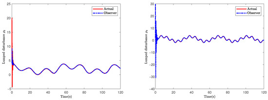
Figure 7. The lumped disturbances and their observations.

Figure 6 displays the curves of the TMR’s velocities. Obviously, the linear and angular velocity observation values can converge to the ones generated by the kinematic controller in fixed time. Figure 7 illustrates that the proposed observer can accurately estimate the system state and compensate for unknown lumped disturbances. It is observed that the proposed control scheme drove the TMR to follow the desired trajectory under the conditions of unknown lumped disturbances. Thus, the proposed control scheme is effective and efficient.

4.2. Tracking Performance in Noise-Polluted Environment

To further validate system robustness, we conducted simulation experiments considering noise $n\left(t\right)$. The above discussion demonstrates the superiority of the FTESO, and the comparison with other observers is omitted here due to space constraints. The simulation results are shown in Figure 8, Figure 9 and Figure 10. Figure 8 demonstrates that the proposed scheme can track the desired trajectory. It is shown in Figure 9 that even in the noise-polluted environment, the proposed model can follow velocities generated by the kinematic controller quickly. By comparing Figure 6 and Figure 9, it is found that the difference in the simulation results is very small between noise-free and noise-polluted situations. However, Figure 10 shows that the control signal curve is not smooth due to high-frequency noise.

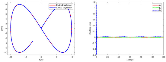
Figure 8. Tracking performance of the proposed model and tracking error considering noise.

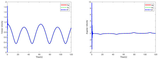
Figure 9. Evolution of TMR linear velocity v and angular velocity $\omega$ considering noise.

Figure 10. Tracking control signals ${\tau }_v$ and ${\tau }_{\omega }$ considering noise.

Next, the convergence time of the system was explored through the comparison between theory and simulation. In view of Theorems 2 and 3, we can calculate the theoretical convergence time in noise-free and noise-polluted environments separately. The comparison results are presented in Table 5.

Table 5. Convergence time validation.

Condition	Theoretical Convergence Time ${}^{\mathit{a}}$		Simulation Convergence Time ${}^{\mathit{b}}$
	Linear Velocity	Angular Velocity	Linear Velocity	Angular Velocity
Noise-free	2.003 s	2.003 s	1.11 s	1.689 s
Noise-polluted	2.003 s	2.003 s	1.115 s	1.693 s

${}^a$ is calculated using (27) and (38). ${}^b$ indicates that the velocity tracking error reaches the ${10}^{-5}$ order.

5. Conclusions

In this paper, a novel FTESO-based FXZNN control scheme is proposed for TMRs. By virtue of the ZNN and extended state observer methods, the proposed control scheme can guarantee that a TMR subject to unmeasured velocities and lumped disturbances precisely tracks the velocity generated by the kinematic controller, as well as the reference trajectory. Additionally, FXZNN model construction with unmeasured velocity is solved using the proposed FTESO. As shown in the simulation experiments, the proposed FTESO can achieve desirable performance when comparing it to the FESO and LESO. In addition, we verified the convergence time of the control model under noise conditions, and the results showed that the convergence time of the model was not affected by noise.

Generally, this paper provides a novel control framework for the trajectory-tracking control of TMRs and successfully extends ZNNs from mobile robot kinematic control to dynamic control, which builds a research bridge from observers to ZNNs. In future works, we would like to conduct physical experiments to verify the effectiveness of the proposed scheme and extend this framework to other similar mobile robots, such as skid-steering mobile robots.

References

- Wang, L.; Wei, H. Avoiding non-Manhattan obstacles based on projection of spatial corners in indoor environment. IEEE/CAA J. Autom. Sin. 2019, 7, 1190–1200. [Google Scholar] [CrossRef]
- Kousik, S.; Vaskov, S.; Bu, F.; Johnson-Roberson, M.; Vasudevan, R. Bridging the gap between safety and real-time performance in receding-horizon trajectory design for mobile robots. Int. J. Robot. Res. 2020, 39, 1419–1469. [Google Scholar] [CrossRef]
- Sun, Z.; Hu, S.; He, D.; Zhu, W.; Xie, H.; Zheng, J. Trajectory-tracking control of mecanum- wheeled omnidirectional mobile robots using adaptive integral terminal sliding mode. Comput. Electr. Eng. 2021, 96, 107500. [Google Scholar] [CrossRef]
- Yu, H.; Sheng, N.; Ai, Z. Sliding mode control for trajectory tracking of mobile robots. In Proceedings of the 40th Chinese Control Conference, Shanghai, China, 26–28 July 2021; pp. 13–17. [Google Scholar]
- Rabbani, M.J.; Memon, A.Y. Trajectory tracking and stabilization of nonholonomic wheeled mobile robot using recursive integral backstepping control. Electronics 2021, 10, 1992. [Google Scholar] [CrossRef]
- Yang, H.; Wang, Z.; Xia, Y.; Zuo, Z. Empc with adaptive apf of obstacle avoidance and trajectory tracking for autonomous electric vehicles. ISA Trans. 2023, 135, 438–448. [Google Scholar] [CrossRef]
- Zhang, J.; Shao, X.; Zhang, W.; Na, J. Path-following control capable of reinforcing transient performances for networked mobile robots over a single curve. IEEE Trans. Instrum. Meas. 2022, 72, 3513312. [Google Scholar] [CrossRef]
- Mai, T.A.; Dang, T.S.; Duong, D.T.; Le, V.C.; Banerjee, S. A combined backstepping and adaptive fuzzy pid approach for trajectory tracking of autonomous mobile robots. J. Braz. Soc. Mech. Sci. Eng. 2021, 43, 1–13. [Google Scholar] [CrossRef]
- Moreno, J.; Slawiñski, E.; Chicaiza, F.A.; Rossomando, F.G.; Mut, V.; Morán, M.A. Design and analysis of an input–output linearization-based trajectory tracking controller for skid-steering mobile robots. Machines 2023, 11, 988. [Google Scholar] [CrossRef]
- Chen, Y.; Li, N.; Zeng, W.; Zhang, S.; Ma, G. Curved path following controller for 4w skid-steering mobile robots using backstepping. IEEE Access 2022, 10, 66072–66082. [Google Scholar] [CrossRef]
- Ge, M.; Xu, H.Z.; Song, Q. Prescribed-time control of four-wheel independently driven skid-steering mobile robots with prescribed performance. Nonlinear Dynam. 2023, 111, 20991–21005. [Google Scholar] [CrossRef]
- Zhang, Y.; Ge, S.S. Design and analysis of a general recurrent neural network model for time-varying matrix inversion. IEEE Trans. Neural. Netw. 2005, 16, 1477–1490. [Google Scholar] [CrossRef] [PubMed]
- Yan, X.; Liu, M.; Jin, L.; Li, S.; Hu, B.; Zhang, X.; Huang, Z. New zeroing neural network models for solving nonstationary sylvester equation with verifications on mobile manipulators. IEEE Trans. Ind. Inform. 2019, 15, 5011–5022. [Google Scholar] [CrossRef]
- Sun, Z.; Shi, T.; Jin, L.; Zhang, B.; Pang, Z.; Yu, J. Discrete-time zeroing neural network of O(τ4) pattern for online solving time-varying nonlinear optimization problem: Application to manipulator motion generation. J. Frankl. Inst. 2021, 358b, 7203–7220. [Google Scholar] [CrossRef]
- Xiao, L.; Jia, L.; Dai, J.; Tan, Z. Design and application of a robust zeroing neural network to kinematical resolution of redundant manipulators under various external disturbances. Neurocomputing 2020, 415, 174–183. [Google Scholar] [CrossRef]
- Li, J.; Zhang, Y.; Mao, M. Continuous and discrete zeroing neural network for different-level dynamic linear system with robot manipulator control. IEEE Trans. Syst. Man Cybern. Syst. 2018, 50, 4633–4642. [Google Scholar] [CrossRef]
- Chen, D.; Li, S.; Wu, Q. A novel supertwisting zeroing neural network with application to mobile robot manipulators. IEEE Trans. Neural Netw. Learn. Syst. 2020, 32, 1776–1787. [Google Scholar] [CrossRef]
- Ma, Z.; Yu, S.; Han, Y.; Guo, D. Zeroing neural network for bound-constrained time-varying nonlinear equation solving and its application to mobile robot manipulators. Neural Comput. Appl. 2021, 33, 14231–14245. [Google Scholar] [CrossRef]
- Zhao, L.; Jin, J.; Gong, J. Robust zeroing neural network for fixed-time kinematic control of wheeled mobile robot in noise-polluted environment. Math. Comput. Simul. 2021, 185, 289–307. [Google Scholar] [CrossRef]
- Chen, D.; Cao, X.; Li, S. A multi-constrained zeroing neural network for time-dependent nonlinear optimization with application to mobile robot tracking control. Neurocomputing 2021, 460, 331–344. [Google Scholar] [CrossRef]
- Jin, J.; Qiu, L. A robust fast convergence zeroing neural network and its applications to dynamic Sylvester equation solving and robot trajectory tracking. J. Frankl. Inst. 2022, 359, 3183–3209. [Google Scholar] [CrossRef]
- Cao, Y.; Liu, B.; Pu, J. Robust control for a tracked mobile robot based on a finite-time convergence zeroing neural network. Front. Neurorobot. 2023, 17, 1242063. [Google Scholar] [CrossRef] [PubMed]
- Zhang, M.; Zheng, B. Accelerating noise-tolerant zeroing neural network with fixed-time convergence to solve the time-varying sylvester equation. Automatica 2022, 135, 109998. [Google Scholar] [CrossRef]
- Li, G.; Lü, J.; Zhu, G.; Liu, K. Distributed observer-based cooperative guidance with appointed impact time and collision avoidance. J. Frankl. Inst. 2021, 358, 6976–6993. [Google Scholar] [CrossRef]
- Silm, H.; Efimov, D.; Michiels, W.; Ushirobira, R.; Richard, J.P. A simple finite-time distributed observer design for linear time-invariant systems. Syst. Control Lett. 2020, 141, 104707. [Google Scholar] [CrossRef]
- Wang, N.; Zhu, Z.; Qin, H.; Deng, Z.; Sun, Y. Finite-time extended state observer-based exact tracking control of an unmanned surface vehicle. Int. J. Robust Nonlinear Control 2020, 31, 1704–1719. [Google Scholar] [CrossRef]
- Fan, Y.; Qiu, B.; Liu, L.; Yang, Y. Global fixed-time trajectory tracking control of underactuated USV based on fixed-time extended state observer. ISA Trans. 2023, 132, 267–277. [Google Scholar] [CrossRef] [PubMed]
- Fan, Y.; Jin, Z.; Luo, X.; Li, S.; Guo, B. Path-Guided Finite-Time Formation Control of Nonholonomic Mobile Robots Based on an Extended State Observer. Appl. Sci. 2022, 12, 9281. [Google Scholar] [CrossRef]
- Roger, M.C. Observer-based proportional integral derivative control for trajectory tracking of wheeled mobile robots with kinematic disturbances. Appl. Math. Comput. 2022, 432, 127372. [Google Scholar]
- Zhang, J.; Yu, S.; Yan, Y. Fixed-time extended state observer-based trajectory tracking and point stabilization control for marine surface vessels with uncertainties and disturbances. Ocean Eng. 2019, 186, 106109. [Google Scholar] [CrossRef]
- Wu, X.; Fei, W.; Wu, X.; Zhen, R. Fixed-time neuroadaptive practical tracking control based on extended state/disturbance observer for a QUAV with external disturbances and time-varying parameters. J. Frankl. Inst. 2022, 359, 3466–3491. [Google Scholar] [CrossRef]
- Wang, S.; Zhai, J. A trajectory tracking method for wheeled mobile robots based on disturbance observer. Int. J. Control Autom. Syst. 2020, 18, 2165–2169. [Google Scholar] [CrossRef]
- Wang, N.; Lv, S.; M, J.E.; Chen, W.H. Fast and Accurate Trajectory Tracking Control of an Autonomous Surface Vehicle With Unmodeled Dynamics and Disturbances. IEEE Trans. Intell. Veh. 2016, 1, 230–243. [Google Scholar] [CrossRef]
- Polyakov, A. Nonlinear feedback design for fixed-time stabilization of linear control systems. IEEE Trans. Autom. Control. 2011, 57, 2106–2110. [Google Scholar] [CrossRef]
- Zheng, Z.; Feroskhan, M.; Sun, L. Adaptive fixed-time trajectory tracking control of a stratospheric airship. ISA Trans. 2018, 76, 134–144. [Google Scholar] [CrossRef] [PubMed]
- Zhang, L.; Wei, C.; Wu, R.; Cui, N. A nonlinear disturbance observer for robotic manipulators. Aerosp. Sci. Technol. 2018, 82–83, 70–79. [Google Scholar] [CrossRef]
- Fukao, T.; Nakagawa, H.; Adachi, N. Adaptive tracking control of a nonholonomic mobile robot. IEEE Trans. Robot. Autom. 2000, 16, 609–615. [Google Scholar] [CrossRef]
- Chen, W.H.; Ballance, D.J.; Gawthrop, P.J.; O’Reilly, J. A nonlinear disturbance observer for robotic manipulators. IEEE Trans. Ind. Electron. 2000, 47, 932–938. [Google Scholar] [CrossRef]
- Gerontitis, D.; Behera, R.; Tzekis, P.; Stanimirović, P. A family of varying-parameter finite-time zeroing neural networks for solving time-varying sylvester equation and its application. J. Comput. Appl. Math. 2022, 403, 113826. [Google Scholar] [CrossRef]
- Wang, H.; Zhang, Y.; Wang, X.; Feng, Y. Cascaded continuous sliding mode control for tracked mobile robot via nonlinear disturbance observer. Comput. Elect. Eng. 2022, 97, 107579. [Google Scholar] [CrossRef]
- Ren, C.; Ding, Y.; Ma, S. A structure-improved extended state observer based control with application to an omnidirectional mobile robot. ISA Trans. 2020, 101, 335–345. [Google Scholar] [CrossRef]
Disclaimer/Publisher’s Note: The statements, opinions and data contained in all publications are solely those of the individual author(s) and contributor(s) and not of MDPI and/or the editor(s). MDPI and/or the editor(s) disclaim responsibility for any injury to people or property resulting from any ideas, methods, instructions or products referred to in the content. |
© 2023 by the authors. Licensee MDPI, Basel, Switzerland. This article is an open access article distributed under the terms and conditions of the Creative Commons Attribution (CC BY) license (https://creativecommons.org/licenses/by/4.0/).