Article

Use of Underwater-Image Color to Determine Suspended-Sediment Concentrations Transported to Coastal Regions

1
Department of Land, Water and Environment Research, Korea Institute of Civil Engineering and Building Technology, Goyang 10825, Republic of Korea
2
Department of Environmental System Engineering, Chonnam National University, Yeosu 59626, Republic of Korea
*
Author to whom correspondence should be addressed.
Appl. Sci. 2023, 13(12), 7219; https://doi.org/10.3390/app13127219
Submission received: 7 May 2023 / Revised: 10 June 2023 / Accepted: 14 June 2023 / Published: 16 June 2023

Abstract

:
The amount of suspended sediment transported from rivers to the ocean fluctuates over time, with a substantial increase occurring during storm events. This surge in sediment poses numerous challenges to coastal areas, highlighting the importance of accurately assessing the sediment load to address these issues. In this study, we developed and experimentally verified a novel method for suspended-sediment-discharge quantification in estuaries and coasts using underwater imaging. Specifically, red clay samples with different particle sizes were introduced into separate tanks containing clean water. After adequate mixing, the concentration, particle size, turbidity, and water quality were measured and analyzed using LISST-200x and EXO2 Multiparameter Sonde sensors. To maintain constant lighting conditions, a camera box was created for filming. Based on the experimental results, a turbidity–concentration relationship formula was derived. The proposed regression equation revealed that the relationship between the turbidity and estimated suspended-sediment concentration was significantly affected by the particle size, and the prediction results were underestimated under high-concentration conditions. Using blue, green, and gray band values, a multiple regression model for estimating suspended-sediment concentrations was developed; its predictions were better than those obtained from the turbidity–concentration relationship. Following efficiency improvements through additional approaches considering underwater-image filming conditions and characteristics of actual streams, estuaries, and coasts, this method could be developed into an easily usable technique for sediment-discharge estimation, helping address sediment-related issues in estuaries and coastal regions.

1. Introduction

The transportation of natural sediments from upland areas to coastal waters generally occurs through rivers. These sediments have significant implications for the coastal ecological environment, coastal disaster prevention, coastal structure management, and coastal sedimentation [1,2,3]. Additionally, the interaction between flow and sedimentation plays a crucial role in the occurrence of scour, which is a prominent hazard and engineering problem for various coastal and river structures [4]. Furthermore, the confluence estuarine zone experiences widespread sediment deposition, leading to the formation of expansive deltaic regions where the riverine and marine environments intersect. However, this process also introduces challenges such as ecosystem stability and increased flooding [5]. Most of the sediment is transported as suspended particles, and the quantity supplied varies over time [6,7,8]. It should be noted that not all transported sediments reach the ocean due to factors such as the large distance and absence of water flow. Maximum transport occurs during flood periods [9]. For instance, in the southeastern Yellow Sea, which lies between China and the Korean Peninsula, the surface concentrations of suspended sediments range from 5 to 100 mg/L, while the bottom concentrations range from 5 to 500 mg/L [10]. This variability is attributed to the late onset of monsoon winds, which allows the sediment generated and transported from rivers during summer rainy seasons to remain stratified [10]. Furthermore, the Yellow Sea is influenced by suspended sediment transported from the Yellow River in China, with an average concentration of approximately 200–1300 mg/L at the river mouth [11,12]. Therefore, the effective management of suspended sediments is vital for addressing erosion, sediment-related problems, and braiding phenomena in estuaries and coastal areas. Accurate identification and interpretation of suspended-sediment concentrations that are transported from rivers to the ocean play a critical role in achieving this management objective. While numerical analysis methods are commonly employed to quantify suspended sediment, their reliability is compromised due to the complex dynamics involving tide, wave action, flow mixing, sediment clumping, sinking, and resuspension [13,14,15]. Consequently, measurements offer the most precise means of determining the amount of sediment spread and the amount that is transported from rivers to the coast.
Several studies have proposed various indirect and direct methods to estimate the concentrations of suspended sediments in estuaries and coastal areas [16,17]. Among these, the direct methods of suspended-sediment concentration measurements involve trap, bottle, pump, and acoustic sampling methods [16]. However, traditional measurement methods such as trap and bottle methods require a significant amount of time and resources and are usually technically difficult. Additionally, they cannot continuously measure sediment concentration. Moreover, when using acoustic profiler equipment, observations are possible only within a limited range of particle diameters. Another disadvantage is that measurements in the presence of bubbles are often difficult [18]. In addition to these, measurement methods using laser diffraction, conductivity, and radiation techniques have been presented; however, these techniques also present evident economic and technical limitations. Owing to these difficulties, various indirect measurement methods have been developed to estimate the concentrations of suspended sand in estuaries and coastal areas. For image-based concentration estimation methods using remote sensing, effective monitoring of the dynamic changes in sediment and suspended matter is feasible. However, such monitoring is possible only in the presence of actually measured floating-matter data, and the efficiency is speculated to be low due to the limited data size. The optical methods are based on the relationship between turbidity and suspended-sediment concentrations through infrared-light scatter, and this method is widely used when direct measurement is difficult. Although this method is economically efficient and facilitates data continuity unlike traditional measurement methods, it presents certain drawbacks. In particular, turbidity is known to vary with the sizes and shapes of sediment particles, and estimating concentrations based on measurements conducted at only one point yields low spatial resolutions [19,20]. Additionally, measurements of the turbidity and concentration of suspended sediments require considering water quality factors aside from sediment characteristics, namely, the salinity of sea water, mineral composition, and the conductivity of nitrogen- or phosphorus species [21,22].
In terms of measuring the concentration of transported suspended sediment, no method can be considered flawless. The monitoring of suspended sediment requires the careful consideration of multiple factors, including concentration range, particle size range, method uncertainty, required reliability, site accessibility, cost, time, and the expertise of personnel involved [17]. In this study, our focus was on an indirect method that utilizes underwater images to estimate sediment concentrations. This approach addresses the limitations observed in previous methods, such as restrictions on particle size and concentration range, while also offering advantages in terms of cost, accessibility, and resolution. Unlike previous proposals for estimating sediment concentrations based on underwater images [23], we employed specially designed equipment in the form of a box to maintain consistent lighting conditions, as these conditions have the most significant impact on underwater image quality. Subsequently, we directly estimated the suspended-sediment concentration by analyzing color variations in these underwater images and compared the results with water quality factors. Through extensive research and experimentation, we have successfully developed a simpler, more efficient, and practical method for estimating suspended-sediment concentrations.

2. Materials and Methods

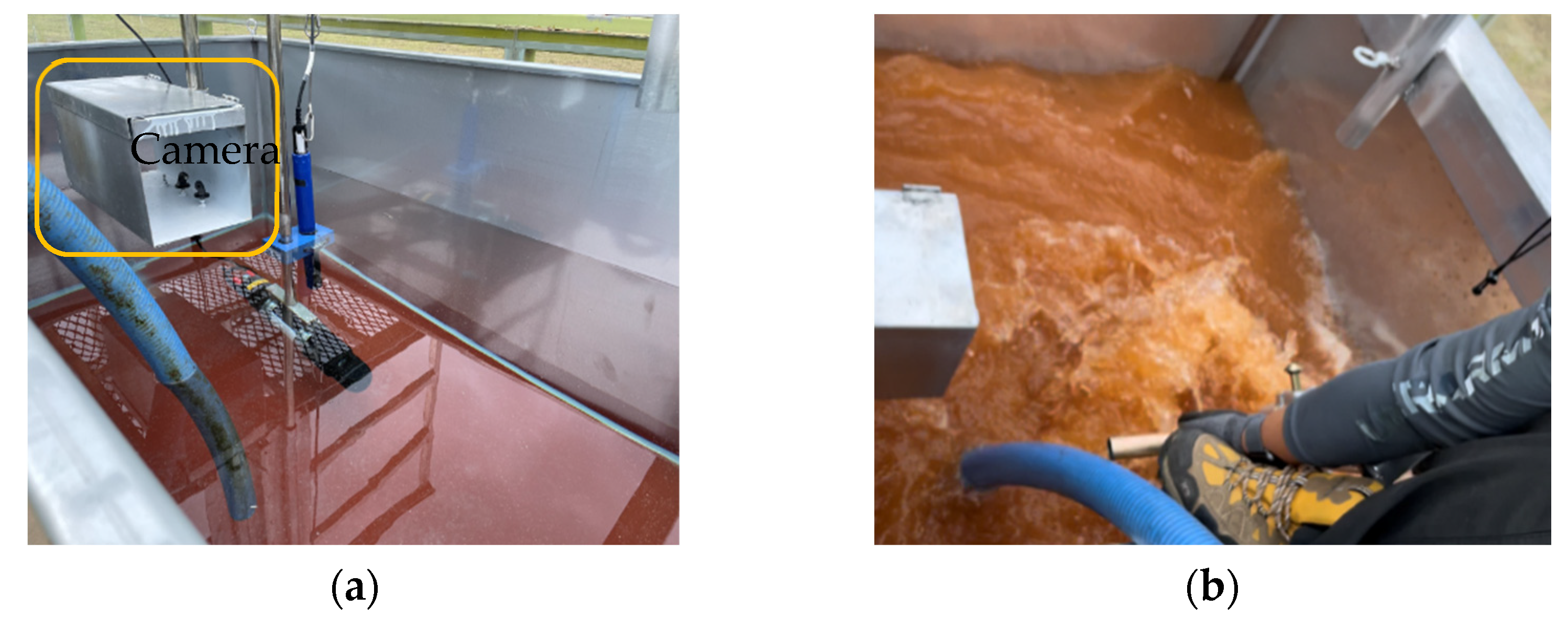
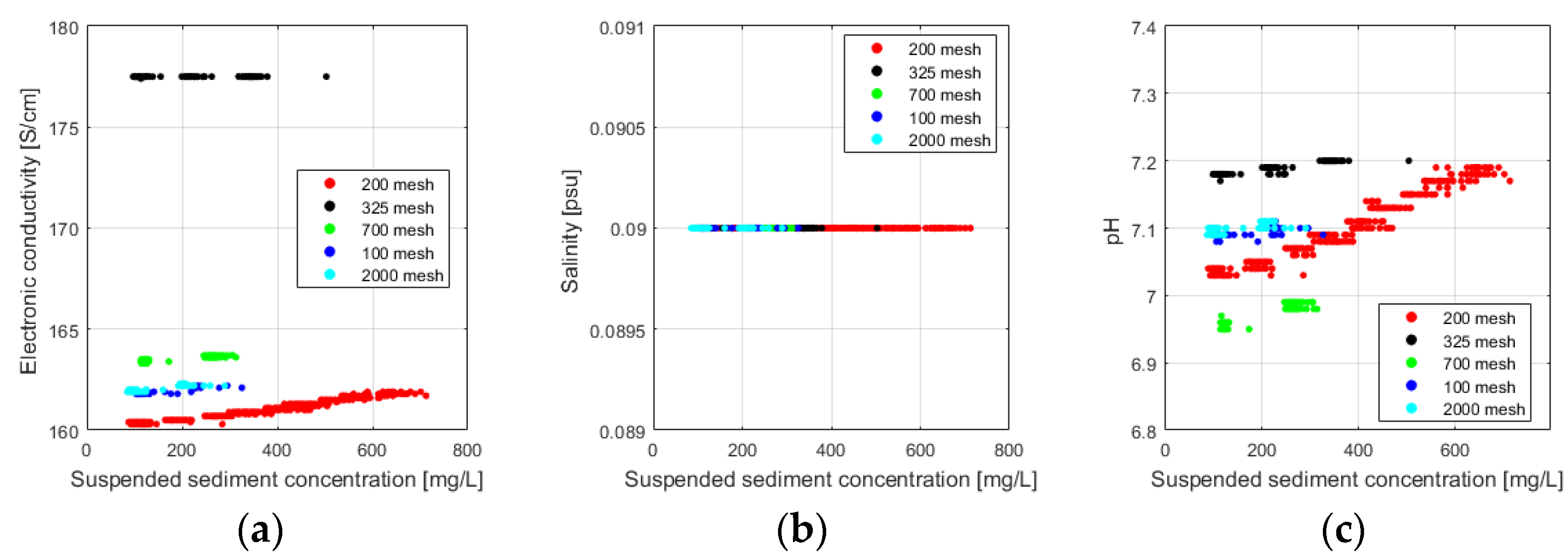
2.1. Experimental Method

The primary objective of this study was to develop an imaging-based method for measuring sediment concentrations; this development required experimental investigations of color changes in underwater images in response to changes in suspended-sediment concentrations. For this, a 1.2 m × 1.8 m water tank was created (Figure 1a).
Five types of red clay (classified by sifting with sieves with mesh sizes of 200, 325, 700, 1000, and 2000) were considered, with each being tested on a different day. In all of the experiments, a water level of 0.695 m (1.5 m3 in volume) was maintained. After 100 g of clay was introduced into the tank, a mixer was used for mixing, thereby simulating the tidal effect in estuaries and coasts. The measurement process was continued while such fluctuations within the water tank were maintained. During the analysis, turbidity and water quality factors were analyzed using a multiparameter water-analysis device—the EXO2 Multiparameter Sonde (EXO2)—and the suspended-sediment concentration and particle size distribution were obtained using the LISST-200x. In this study, the concentration of suspended sediment measured by the LISST device was considered the true concentration and used as the calibration value for developing our model, as it is unaffected by the particle size distribution [17]. Moreover, to ensure accurate measurements and eliminate discrepancies, both devices were installed at the same height (a 0.3 m water depth), and the bed condition in the water tank remained constant throughout the measurement period, effectively minimizing any potential impact of sensor alignment or changes in the bed condition on the measurement results [24,25].
Generally, when using the indirect method of concentration estimation using turbidity, sufficient consideration of salinity, mineral composition, nitrogen or phosphorus species, and conductivity is required [21,22]. Notably, in this study, relatively clean water was used to maintain water quality conditions, and EXO2 was used to determine the turbidity and other parameters, such as the electronic conductivity, salinity, and potential of hydrogen (pH) every second to verify the water quality. Note that an LISST-200x sediment sensor is capable of measuring the volume concentration and suspended-sediment particle size (1.00–5000 microns) every second and assessing the reliability of the obtained results based on transmission values, which represent the probability of multiple scattering. If these measured transmission values are 0.1 or less after the red clay addition, the experiment is terminated as reliability can no longer be ensured. To account for the variation in lighting with time and water depth, a Go-Pro 9 camera and underwater light source were installed in the camera box to continuously record underwater images under constant illumination from a light source (Figure 1). During the experiment, the camera box was carefully installed parallel to the other equipment, ensuring proper alignment, and was positioned at the same height. Images were captured every second. From other underwater images, the dependence of the red/green/blue (RGB) and gray band values on the suspended-sediment concentration was identified.

2.2. Analysis Method

Notably, the turbidity and suspended-sediment concentration are closely related; however, standard conventions for calibrating methods are yet to be proposed [26]. The turbidity is an optical property of water, and water transparency is known to decrease in the presence of undissolved particles. This can be commonly observed using nephelometry [27]. Overall, to estimate the concentrations of suspended sediments more accurately, establishing a precise relationship between the two is essential. However, a single accurate formal method for obtaining this turbidity–concentration relationship is not available; therefore, three commonly employed forms were adopted here: (1) the power law, (2) second-order polynomial, and (3) first-order polynomial. In a recent study, turbidity was predicted based on water color changes (RGB value), following which the suspended-sediment concentration was estimated based on the predicted turbidity [23]. In this study, a multilinear regression model that could directly predict the change in concentration based on color change was developed. In particular, after analyzing the relationship between concentration and turbidity, a model was developed using the form presenting the best correlation. Finally, the suspended-sediment concentration predicted by the model was compared with other predictions based on the turbidity–concentration relationship. The developed multiple regression models were evaluated based on the root-mean-square error (RMSE) (Equation (1)), and the variance inflation factor (VIF) in multicollinearity problems was calculated using Equation (2).
R M S E = 1 n i = 1 n ( x i y i ) 2
V I F = 1 1 R 2

3. Results

The data collected over five experiments were deemed sufficient to establish a relationship between the concentration and turbidity, which is used in the existing methods, and underwater-image color change, which is used in the proposed method.

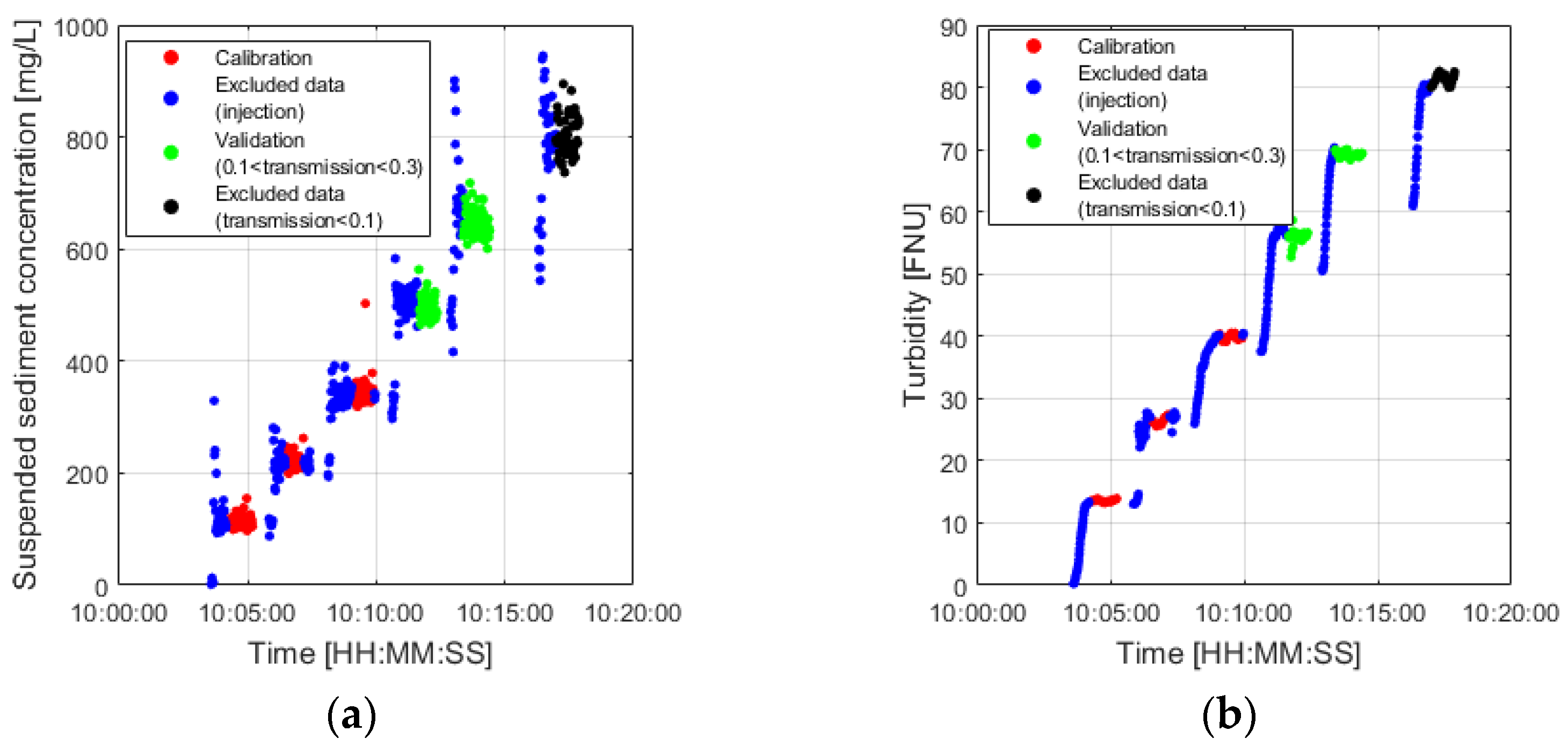
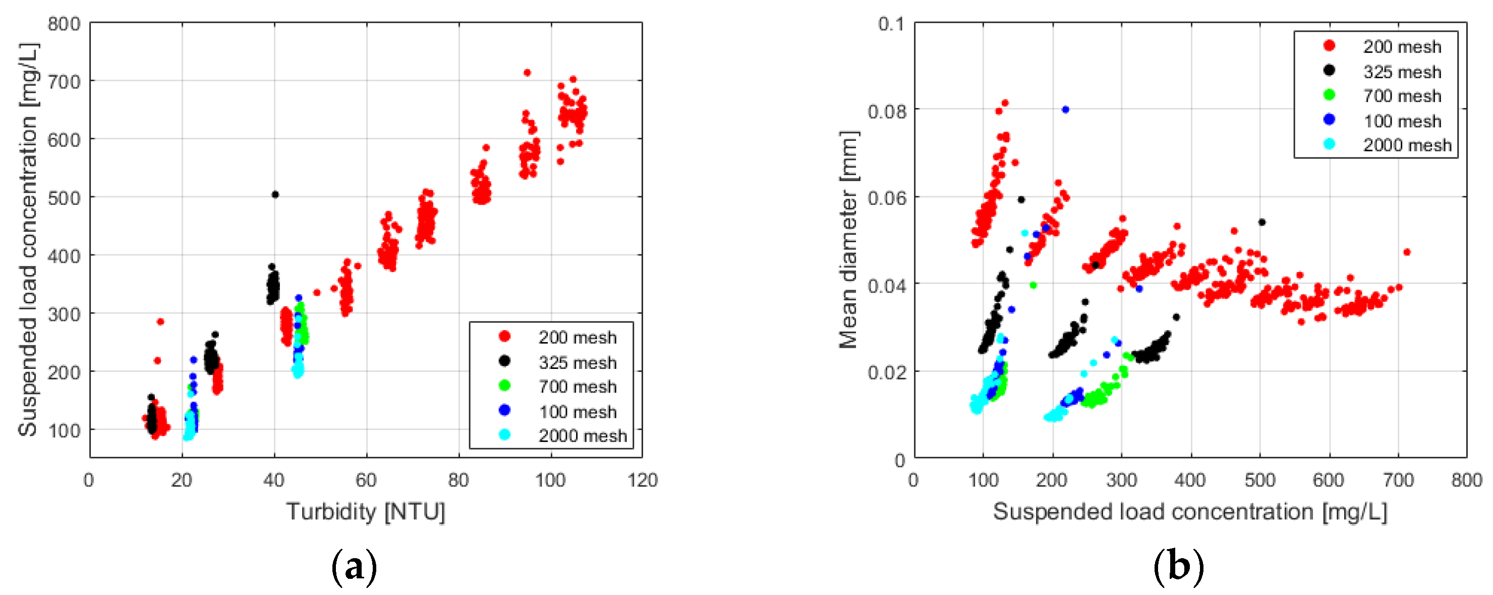
3.1. Turbidity vs. Sediment Concentration

The water quality results obtained from five independently conducted experiments for each suspended-sediment particle size are depicted in Figure 2. Notably, the red clay sieved with a 200 mesh appeared to include impurities that affected the electrical conductivity, and the alkalinity of the mixture increased slightly with increasing concentrations due to lime or magnesium oxide present in the red clay (Figure 2a,c).
The obtained values of the water quality factors did not differ significantly, indicating that the experimental conditions remained constant. This implied that the other factors affecting the relationship between water color, turbidity, and suspended concentration were well controlled. In the five experiments, 1044, 595, 520, 419, and 318 measurement results were obtained in total. The measurement results obtained during the addition of the suspended sediments presented a transmission value of less than 0.1; therefore, these 968 data points were considered nonreliable and were excluded from the analysis (Figure 3). Additionally, 489 data points (0.1 < transmission value < 0.3) that required caution were compared with the results used in the analysis and were considered as validation data because the concentration increased consistently after the addition of 100 g of red clay. In coastal waters, a significant proportion of particles exist as flocs or aggregates, which are clusters of several particles connected together to form a single entity through the tidal effect [28].
When the mixer was in operation, the measured sediment concentration was found to be more than twice as high compared to the measurements taken when the mixer was turned off and the fluctuation was maintained. This observation strongly indicates that flow conditions, such as tidal patterns, waves, and mixing processes in coastal areas and estuaries, have a substantial influence on concentration measurements. Consequently, the continuous monitoring and collection of measurement data are essential in coastal regions to account for these dynamic factors. To identify the effect of the particle size of red clay and the inclusion of substances other than red clay on the suspended-sediment concentration, the particle size distribution of the suspended sediment recorded using the LISST-200X every second was compared with that of the red-clay-only specimen recorded using the BW-tube method (Figure 4).
The particle size distribution results obtained with the BW method (red line) significantly differed from the measurement results (dotted line) that were excluded from the analysis owing to data reliability issues or measurements during the red clay addition. We confirmed that the smaller the particle size, the greater the proportion of data to be excluded from the analysis. Furthermore, the analysis of the excluded data revealed that the reliability of the results obtained from the LISST-200x device was unsatisfactory. The particle size distribution curves derived from these measurements indicated that the instrument consistently underestimated the presence of particles, which is consistent with findings from other studies [29]. However, the two other methods employed in this study did not exhibit such a significant discrepancy and yielded acceptable results. In addition, sieving red clay with a 700 or smaller mesh was found to not produce a difference in the particle size. Red clay in units of 100 g was added nine times with the 200 mesh, three times with the 325 mesh, and two times in the remaining cases until the transmission value became 0.3 or less. The turbidity–concentration relationships derived from the experimental results were found to significantly differ for different particle sizes (Figure 5).

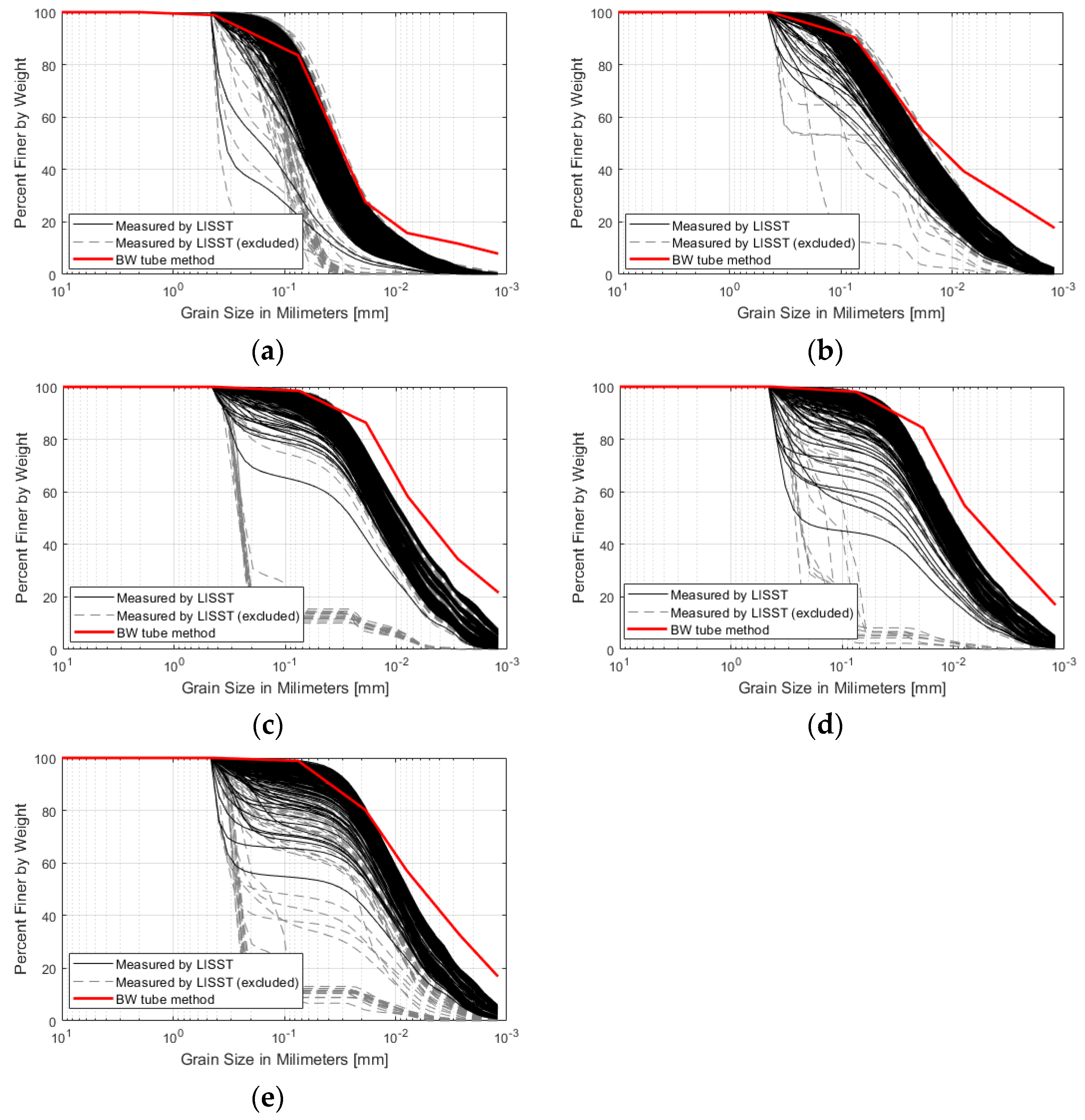
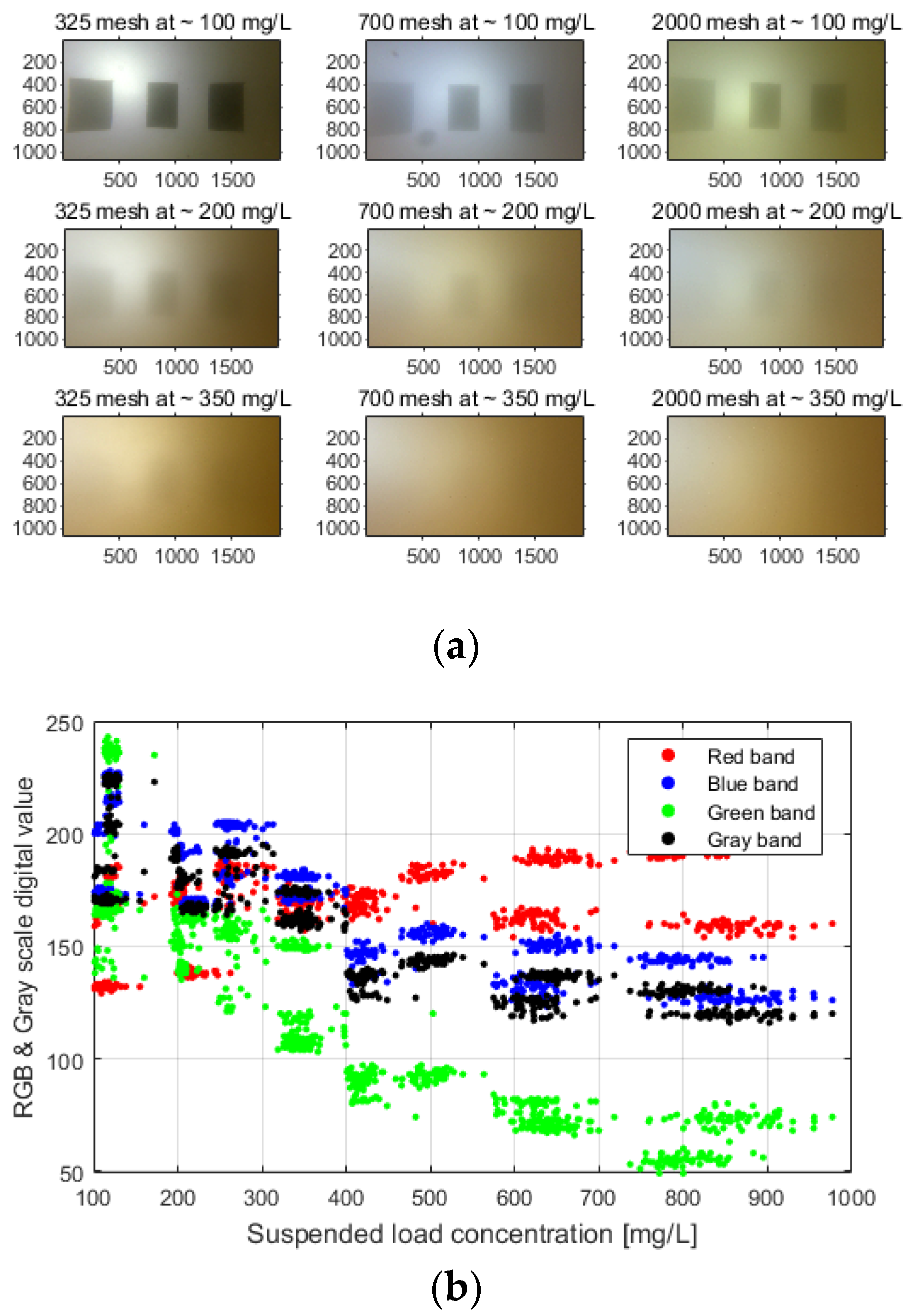
3.2. Underwater-Image Color vs. Sediment Concentration

The 200 and 1000 mesh experiments were excluded from the analysis because an insufficiency in the power supply resulted in a failure to maintain constant lightning conditions. Underwater images for similar concentrations in the 325, 500, and 2000 mesh experiments are presented in Figure 6a.
At low concentrations, color variations were observed across the samples, depending on the light-source and filming conditions; these differences became smaller as the concentration increased. To quantitatively analyze these color changes, the RGB band value that changed as compared to the pixel and the corresponding change in the gray band value was identified (Figure 6b). This study (in contrast to previous research [14]) identified that the red band value was the most sensitive among the different light wavelengths of underwater images and varied irregularly with the concentration. This result may be attributed to the complex impacts of the underwater lighting system and the introduction of the red-colored clay. The values of the other bands decreased as the concentration increased; notably, that of the green band rapidly decreased.

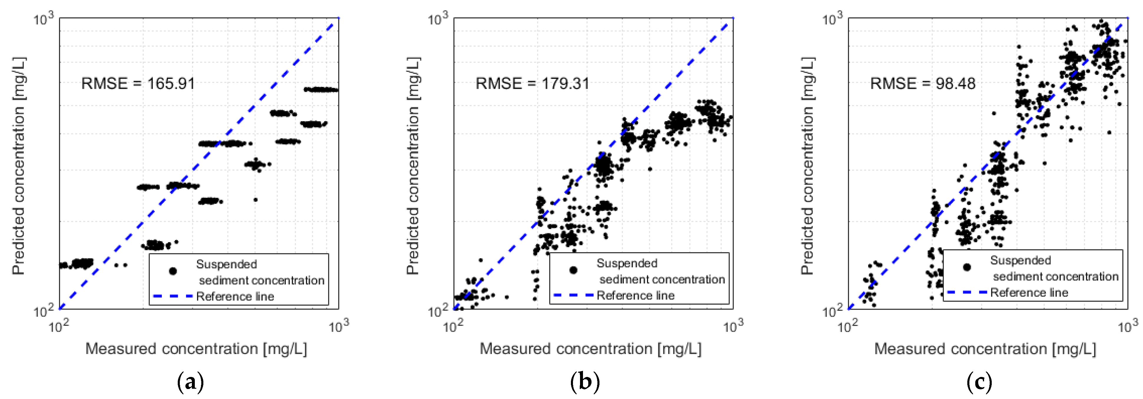
3.3. Comparison with Turbidity-Based Predictions

First, three turbidity–concentration relationships were analyzed to determine the form of the model to be used for predicting suspended-sediment concentrations based on color changes (Table 1).
The power law turbidity–concentration relationship formula presented the greatest correlation (R2 = 0.66). Therefore, a log-transformed multiple regression model was developed for estimation of the suspended-sediment concentration Csus (Table 2).
Additionally, a multiple regression model predicting turbidity based on color change was developed (Table 3).
The model predicting concentrations from color changes presented a higher R2 value than the model predicting turbidity. This was speculated to occur because the range of measured concentrations was wider than that of turbidity. Because multiple regression models are required to be aware of the problem of multicollinearity, the VIF value for each model was analyzed. Furthermore, because the gray value was generated based on the combination of RGB, regression models that included gray-scale values provided extremely high multicollinearity (VIF > 10). Finally, the values of Csus that were estimated based on the turbidity, predicted turbidity, and underwater-image color were compared (Figure 7).
The RMSE in Csus obtained from the underwater-image color change was 99 mg L−1, which was better than that obtained from the measured turbidity (~166 mg L−1) and predicted turbidity (~180 mg L−1). The prediction based on the measured turbidity was reconfirmed to be affected by the particle size of the suspended sediment. On comparison, the concentration predicted from the high-concentration validation section of the model predicting turbidity tended to be significantly smaller than the measurement results. This indicates that the concentrations predicted based on turbidity are not appropriate for predictions of an unmeasured range value.

4. Discussion

A previous study [23] predicted turbidity based on color changes in an underwater image that was captured directly (without a specific light-source supply) in a single-case experiment; following this, the direct relationship between turbidity and concentration was used to estimate the suspended-sediment concentration. In the present study, similar results were obtained under constant lighting conditions even when the underwater filming conditions were dynamic. Moreover, the concentration was directly estimated based on color changes, overcoming the limitations associated with the turbidity–concentration relationship.
Generally, most turbidity measurement methods utilize scattering rates due to turbid particles; therefore, the obtained results depend on the shapes and sizes of suspended-sediment particles. Additionally, the forms of the equations exert a dominant influence on the indirect methods of concentration estimation based on the turbidity–concentration relationship during the estimation of a section that was not involved in creating the formula. Therefore, the exponent (0.85) of the turbidity–concentration relationship equation proposed in this study was found to be lower than one, and the predicted values were low at high concentrations. In contrast, the underwater-image color change observed in this study was not significantly impacted by the particle size and yielded better predictions compared to the turbidity–concentration relationship.
Based on the developed models, the red and green band values could be deemed critical for predicting suspended-sediment concentrations because the models included two of the best band-provided R2 values between the models with two explanatory variables. These results can be attributed to the following phenomena: The wavelength that can penetrate the deepest in water changes from blue to green because particles tend to mostly absorb blue light, whereas water is known to absorb red light. In addition, coastal waters typically contain mineral or clay particles with a high refractive index, making them very efficient at scattering light [17]. In this study, the underwater-image color was observed to differ under different experimental cases at low concentrations. While the overall range of predicted results demonstrated good predictability, the accuracy of predictions at low concentrations was lower compared to that of the turbidity–concentration relationship. Since coastal regions typically exhibit very low suspended-sediment concentrations, it is recommended to utilize the suggested method in conjunction with existing measurement methods. To enhance predictability at low concentrations, further analysis and experimentation should be conducted.
The estimation of sediment concentrations may also be influenced by various filming and image-related conditions, such as lens state and camera performance. The lower predictability at low concentrations suggests the need for improvements in the camera box system to ensure consistent light-source conditions. In future research, the camera box will be redesigned to prevent any refracted light from entering through the water surface, thus maintaining constant lighting conditions. Additionally, a method that considers factors such as contrast and brightness, beyond just the RGB values, will be developed for estimating suspended-sediment concentrations. Moreover, for the application of the proposed method to real estuaries or coastal areas, additional parameters and experiments need to be considered. The experiments conducted in this study were carried out under constant conditions; however, further experiments accounting for different flow conditions and changes in water quality factors such as salinity are necessary. Furthermore, our study solely focused on red clay, and additional research using different types of sand, silt, and clay is warranted. The single-point sampling method may not be efficient due to flocculation in muddy estuaries and the influence of tidal effects on coastal areas. The suggested method, utilizing underwater imaging, holds the potential to estimate suspended-sediment concentrations throughout the water column over a wide range.

5. Conclusions

This paper proposes the use of underwater-image color changes to quantitatively estimate suspended-sediment discharge, which is essential to solve various issues related to sedimentation on coasts or in rivers or estuaries. In an experiment, 100 g of red clay samples that were classified into five different types based on particle size (200, 325, 700, 1000, and 2000 mesh) were introduced into water tanks with dimensions of 1.2 × 1.8 m. Every second, the concentration, turbidity, suspended-sediment particle size, underwater images, and water quality factors were recorded using the LISST-200x, EXO2 Multiparameter Sonde, and a Go-Pro camera. Of the 2958 data points, 968 with low reliability or those measured during the introduction of the suspended sediment were excluded from the analysis, and 489 points were used for the validation of the suspended-sediment concentration estimation model. For the underwater images, an underwater light source installed within the camera box supplied constant light during image recording. The underwater images of the 325, 700, and 2000 mesh samples were analyzed and used for subsequent model development.
Because turbidity is typically measured according to the scattering rate, the particle size of the suspended sediments was expected to significantly impact the turbidity–concentration relationship. Next, three most commonly used forms of the turbidity–concentration relationship were applied to the experimental results. Among these, the power law form presented the highest correlation (R2 = 0.66). To identify color changes in the underwater image according to concentration changes based on the supplied pixels from the light source, the RGB and gray band value changes were observed. For all of the bands except red, the values tended to decrease as the concentration increased. Finally, the analyzed band values were used to develop a log-transformed multiple regression model for turbidity and suspended-sediment-concentration prediction. The validation and calibration datasets were utilized to compare the suspended-sediment-concentration predictions with those obtained from the turbidity–concentration relationship and the concentration predicted by the turbidity from the predicted turbidity model. The concentrations obtained from the predicted turbidity model were significantly low in the validation data section under high-concentration conditions (RMSE = 180 mg L−1). In contrast, the suspended-sediment concentration that was estimated based on underwater-image color changes was not affected by the particle size, and the prediction was reliable, even at high concentrations (RMSE = 99 mg L−1). The method proposed in this paper allows for steady monitoring and could be more efficient and easier to use compared with the existing methods. To ensure practical applicability of the proposed method, establishing a connection with existing measurement methods is crucial. Furthermore, additional experiments and research will contribute to the further development of this method as a practical approach for quantifying suspended-sediment discharge. Such a method will play a valuable role in addressing sediment-related challenges in estuaries and coastal areas.

Author Contributions

Conceptualization, W.K. and S.K.; formal analysis, W.K., K.L. and S.K.; writing—review and editing, W.K. and S.K. All authors have read and agreed to the published version of the manuscript.

Funding

This research was supported by a National Research Foundation of Korea (NRF) grant that was funded by the Korean government (No. 2021R1C1C101040411).

Institutional Review Board Statement

Not applicable.

Informed Consent Statement

Not applicable.

Data Availability Statement

Not applicable.

Acknowledgments

This study used an experimental infrastructure at the River Experiment Center of the Korea Institute of Civil Engineering and Building Technology.

Conflicts of Interest

The authors declare no conflict of interest.

References

  1. Lin, B.; Falconer, R.A. Numerical modelling of three-dimensional suspended sediment for estuarine and coastal waters. J. Hydraul. Res. 1996, 34, 435–456. [Google Scholar] [CrossRef]
  2. Shin, B.S.; Kim, K.H. Prediction of environmental change and mitigation plan for large scale reclamation. J. Korean Soc. Coast. Ocean Eng. 2010, 22, 95–100. [Google Scholar]
  3. Jeong, J.H.; Tac, D.H.; Lim, J.H.; Lee, D.I. Analysis and improvement for impact assessment of suspended solids diffusion by marine development projects. J. Korean Soc. Mar. Environ. Energy 2017, 20, 160–171. [Google Scholar] [CrossRef]
  4. Chiew, Y.-M.; Lai, J.-S.; Link, O. Experimental, Numerical and Field Approaches to Scour Research. Water 2020, 12, 1749. [Google Scholar] [CrossRef]
  5. Khan, M.A.; Sharma, N.; Pu, J.H.; Pandey, M.; Azamathulla, H. Experimental Observation of Turbulent Structure at Region Surrounding the Mid-Channel Braid Bar. Mar. Georesour. Geotechnol. 2022, 40, 448–461. [Google Scholar] [CrossRef]
  6. Kang, W.; Jang, E.K.; Yang, C.Y.; Julien, P.Y. Geospatial analysis and model development for specific degradation in South Korea using model tree data mining. Catena 2021, 200, 105142. [Google Scholar] [CrossRef]
  7. Kang, W.; Lee, K.; Jang, E.K. Evaluation and validation of estimated sediment yield and transport model developed with model tree technique. Appl. Sci. 2022, 12, 1119. [Google Scholar] [CrossRef]
  8. Yang, C.Y.; Kang, W.; Lee, J.H.; Julien, P.Y. Sediment regimes in South Korea. River Res. Appl. 2022, 38, 209–221. [Google Scholar] [CrossRef]
  9. Eisma, D. Suspended Matter in the Aquatic Environment; Springer Science & Business Media: Berlin, Germany, 2012. [Google Scholar]
  10. Wells, J.T. Distribution of Suspended Sediment in the Korea Strait and Southeastern Yellow Sea: Onset of Winter Monsoons. Mar. Geol. 1988, 83, 273–284. [Google Scholar] [CrossRef]
  11. Lin, H.; Yu, Q.; Wang, Y.; Gao, S. Identification, Extraction and Interpretation of Multi-Period Variations of Coastal Suspended Sediment Concentration Based on Unevenly Spaced Observations. Mar. Geol. 2022, 445, 106732. [Google Scholar] [CrossRef]
  12. Cai, L.; Chen, S.; Yan, X.; Bai, Y.; Bu, J. Study on High-Resolution Suspended Sediment Distribution under the Influence of Coastal Zone Engineering in the Yangtze River Mouth, China. Remote Sens. 2022, 14, 486. [Google Scholar] [CrossRef]
  13. Amoudry, L.O.; Souza, A.J. Deterministic coastal morphological and sediment transport modeling: A review and discussion. Rev. Geophys. 2011, 49, 1–21. [Google Scholar] [CrossRef] [Green Version]
  14. Lisit͡syn, A.P. Sedimentation in the World Ocean with Emphasis on the Nature, Distribution and Behavior of Marine Suspensions; Society of Economic Paleontologists and Mineralogists: Tulsa, OK, USA, 1972; Volume 17. [Google Scholar]
  15. Kravchishina, M.D.; Lisitsyn, A.P.; Klyuvitkin, A.A.; Novigatsky, A.N.; Politova, N.V.; Shevchenko, V.P. Suspended Particulate Matter as a Main Source and Proxy of the Sedimentation Processes. In Sedimentation Processes in the White Sea: The White Sea Environment Part II; Springer: Berlin/Heidelberg, Germany, 2018; pp. 13–48. [Google Scholar]
  16. White, T.E. Status of measurement techniques for coastal sediment transport. Coast. Eng. 1998, 35, 17–45. [Google Scholar] [CrossRef]
  17. Felix, D.; Albayrak, I.; Boes, R.M. Continuous Measurement of Suspended Sediment Concentration: Discussion of Four Techniques. Measurement 2016, 89, 44–47. [Google Scholar] [CrossRef]
  18. Siadatmousavi, S.M.; Jose, F.; Chen, Q.; Roberts, H.H. Comparison between Optical and Acoustical Estimation of Suspended Sediment Concentration: Field Study from a Muddy Coast. Ocean Eng. 2013, 72, 11–24. [Google Scholar] [CrossRef]
  19. Hatcher, A.; Hill, P.; Grant, J.; Macpherson, P. Spectral optical backscatter of sand in suspension: Effects of particle size, composition and colour. Mar. Geol. 2000, 168, 115–128. [Google Scholar] [CrossRef]
  20. Merten, G.H.; Capel, P.D.; Minella, J.P. Effects of suspended sediment concentration and grain size on three optical turbidity sensors. J. Soils Sediments 2014, 14, 1235–1241. [Google Scholar] [CrossRef]
  21. Sun, Z.L.; Jiao, J.G.; Huang, S.J.; Gao, Y.Y.; Ho, H.C.; Xu, D. Effects of suspended sediment on salinity measurements. IEEE J. Ocean. Eng. 2017, 43, 56–65. [Google Scholar] [CrossRef]
  22. Leigh, C.; Kandanaarachchi, S.; McGree, J.M.; Hyndman, R.J.; Alsibai, O.; Mengersen, K.; Peterson, E.E. Predicting sediment and nutrient concentrations from high-frequency water-quality data. PLoS ONE 2019, 14, e0215503. [Google Scholar] [CrossRef] [Green Version]
  23. Kang, W.; Lee, K.; Kim, J. Prediction of suspended sediment concentration based on the turbidity-concentration relationship determined via underwater image analysis. Appl. Sci. 2022, 12, 6125. [Google Scholar] [CrossRef]
  24. Pu, J.; Wei, J.; Huang, Y. Velocity Distribution and 3D Turbulence Characteristic Analysis for Flow over Water-Worked Rough Bed. Water 2017, 9, 668. [Google Scholar] [CrossRef] [Green Version]
  25. Pu, J.H. Velocity Profile and Turbulence Structure Measurement Corrections for Sediment Transport-Induced Water-Worked Bed. Fluids 2021, 6, 86. [Google Scholar] [CrossRef]
  26. Minella, J.P.G.; Merten, G.H.; Reichert, J.M.; Clarke, R.T. Estimating Suspended Sediment Concentrations from Turbidity Measurements and the Calibration Problem. Hydrol. Process 2008, 22, 1819–1830. [Google Scholar] [CrossRef] [Green Version]
  27. Lawler, D.M.; Petts, G.E.; Foster, I.D.L.; Harper, S. Turbidity Dynamics during Spring Storm Events in an Urban Headwater River System: The Upper Tame, West Midlands, UK. Sci. Total Environ. 2006, 360, 109–126. [Google Scholar] [CrossRef] [PubMed]
  28. Bowers, D.G. Optical Techniques in Studying Suspended Sediments, Turbulence and Mixing in Marine Environments. In Subsea Optics and Imaging; Elsevier: Amsterdam, The Netherlands, 2013; pp. 213–240. ISBN 9780857093417. [Google Scholar]
  29. Gartner, J.W.; Cheng, R.T.; Wang, P.-F.; Richter, K. Laboratory and Field Evaluations of the LISST-100 Instrument for Suspended Particle Size Determinations. Mar. Geol. 2001, 175, 199–219. [Google Scholar] [CrossRef]
Figure 1. (a) Experimental water tank and measurement devices and (b) mixing after addition of suspended sediment.
Applsci 13 07219 g001
Figure 2. Measurement results for the (a) electronic conductivity, (b) salinity, and (c) acidity (pH).
Applsci 13 07219 g002
Figure 3. Measurement results of (a) concentration and (b) turbidity in the 325 mesh experiment.
Applsci 13 07219 g003
Figure 4. Particle size of the suspended sediment obtained using the LISST-200x sensor and grain-size distribution obtained using the BW-tube method: (a) 200 mesh, (b) 325 mesh, (c) 700 mesh, (d) 1000 mesh, and (e) 2000 mesh.
Applsci 13 07219 g004
Figure 5. Results of the (a) concentration as a function of turbidity and (b) diameter as a function of concentration for each particle size.
Applsci 13 07219 g005
Figure 6. Changes in the (a) color of the underwater image and (b) RGB and gray band values in response to changes in the suspended-sediment concentration.
Applsci 13 07219 g006
Figure 7. Suspended-sediment concentration estimated from (a) the measured turbidity, (b) predicted turbidity, and (c) underwater-image color change.
Applsci 13 07219 g007
Table 1. Concentration Csus from turbidity tur based on three methods.
TypeEquationR2
Power law C s u s = 10.29 · t u r 0.85 0.66
Second-order
polynomial
C s u s = 0.13 · t u r 2 + 13.84 · t u r + 85.16 0.61
First-order polynomial C s u s = 5.5 · t u r + 24.91 0.63
Table 2. Model for predicting concentration from color change.
EquationR2Highest VIF
C s u s = 179.82 × R 5.23 × G 10.45 × B 0.23 × g r a y 5.54 0.82102.16
C s u s = 327.41 × R 5.23 × G 7.29 × B 0.4 0.819.54
C s u s = 3498.18 × R 4.56 × G 5.11 0.801.11
C s u s = 3.44 × 10 4 × R 0.59 × B 1.66 0.671.16
C s u s = 1.97 × 10 7 × G 0.77 × B 1.54 0.681.99
Table 3. Model predicting turbidity from color change.
EquationR2Highest VIF
T u r b i d i t y N T U = 74.67 + 0.36 · R 2.91 · G 0.69 · B + 2.83 · G r a y 0.82250
T u r b i d i t y N T U = 81.16 + 1.13 · R 1.45 · G + 0.12 · B 0.738.89
T u r b i d i t y N T U = 87.15 + 0.99 · R 1.45 · G 0.721.11
T u r b i d i t y N T U = 104.21 + 0.09 · R 0.59 · B 0.621.12
T u r b i d i t y N T U = 74.67 2.91 · G 0.69 · B 0.632.13
Disclaimer/Publisher’s Note: The statements, opinions and data contained in all publications are solely those of the individual author(s) and contributor(s) and not of MDPI and/or the editor(s). MDPI and/or the editor(s) disclaim responsibility for any injury to people or property resulting from any ideas, methods, instructions or products referred to in the content.

