A Good Practice for the Proof Testing of Cable-Stayed Bridges

Featured Application

The paper presents the significance of a comprehensive experimental campaign, including static and dynamic tests, for the proof testing of cable-stayed bridges, aimed at the development of a reliable digital twin model of the structure for health monitoring purposes.

Abstract

This paper presents the results and interpretations of static and dynamic tests that were executed on a newly built cable-stayed steel-concrete composite bridge during the final proof testing. A brief description of the structure, the testing methodology, and the used instrumentation are presented. Then, the test results are widely discussed and interpreted in order to evaluate the bridge performance during the proof test and also to understand the usefulness of each performed test in a proof test framework. All the collected experimental data are also compared to the numerical ones that were obtained through a refined finite element model, in order to check the behavior of the structure. The outcomes of the present work can offer references for the proof testing and monitoring of cable-stayed bridges.

1. Introduction

Studies on the static and dynamic behavior of cable-stayed bridges reveal that they are quite complex systems in which the experimental control of the structure compliance with the design schemes is crucial not only for the final proof test, that is necessary before the opening to traffic, but also during the bridge construction. For example, the deck launching is usually studied and controlled through staged analyses that are able to account for the progressive loading of stays, and the experimental verification of such forces may be crucial to obtain the final desired deck longitudinal profile. At the same time, the final proof test of cable-stayed bridges should not be limited to the control of the deck deformability, and a sufficient number of tests should be planned to check the overall static and dynamic behavior of the complex structural system.

Several works in the literature focus on proof testing of cable-stayed bridges through dynamic and static tests. For example, Gomez-Martinez et al. [1] presented the experimental response of two newly built cable-stayed bridges in Mexico that were subjected to static and dynamic loads, addressing the use of optical fiber sensors to perform the bridge monitoring during the tests. Also, Bayraktar et al. [2] showed static, ambient, and dynamic field test observations of the long span Nissibi cable-stayed bridge in Turkey, while Liu et al. [3] discussed the static and dynamic tests that were performed on the Suifenhe cable-stayed bridge (China) after 12 years from its opening to traffic, with the aim of evaluating its health status. Other works only focus on results of static proof load tests before the bridge opening to traffic, such as for the Redzinski bridge in Wroclaw [4] and the Kao-Ping-Hsi bridge in Taiwan [5]. On the contrary, some works only deal with dynamic tests that were performed on the whole structure, such as for the Alamillo bridge in Sevilla [6], the Indiano bridge in Florence [7], the Vasco da Gama bridge in Portugal [8], and the Colquitz river bridge in Canada [9]. Furthermore, some works are also available in the literature dealing with the behavior of single components of bridges, such as those investigating the behavior of stay cables under severe weather [10] or temperature conditions [11], or those studying their tension forces [12] adopting dynamic tests.

Concerning the usefulness of tests, many authors adopted in situ experimental campaigns to support the updating procedures of the investigated bridge numerical model; some examples in this sense are the works on the Yong river bridge [13], the Ting Kau bridge [14], and the Chongqin bridge [15] in China, the Porto Marghera bridge in Italy [16], and the famous Stonecutters bridge in Hong Kong [17].

Moreover, in the work of Alamdari et al. [18] a new method for bridge damage detection that is based on a combined experimental and numerical procedure is proposed. Very recent works are also available in the literature dealing with innovative and unconventional methods to test cable-stayed bridges (and also bridges in general). For example, Lee et al. [19] and Yu et al. [20] proposed new vision-based procedures to perform measurement displacements through high-resolution cameras, testing their procedure on real case studies, such as the Cheonsa bridge in South Korea, and the Su Tong Yangtze river bridge in China. Furthermore, Miccinesi, and Pieraccini [21] proposed an interferometric radar that was able to investigate the dynamic behavior of bridges and they tested their methodology on the new Arno river bridge in Italy.

Finally, some interesting works deal with the static and dynamic monitoring of important cable-stayed bridges all around the world, such as the Millau viaduct in France [22], the Basarab bridge in Romania [23], and the Jindo bridge in South Korea [24].

Starting from the above literature review on proof testing of cable-stayed bridges, this paper presents the extensive experimental campaign that was performed by the authors during the proof load test of a newly built cable-stayed bridge (the Filomena Delli Castelli bridge), with the aim of providing useful suggestions for practitioners and developing a good practice for the proof testing of cable-stayed bridges. In detail, many types of static and dynamic tests have been performed to control the response of the bridge members (e.g., deck, pylons, and support devices) at loaded and unloaded conditions and also to understand their usefulness during the proof test. The latter were defined on the basis of the design finite (FE) element model. Moreover, a refined FE model of the whole bridge has been developed with a twofold aim: (i) to interpret experimental test outcomes and, at the same time, to verify the compliance of the real bridge behavior with the numerically predicted one; and (ii) to support the development of a digital twin of the real structure to be used in the future as benchmark for monitoring changes in the bridge structural behavior.

The paper contents are organized as follows: Section 2 reports a comprehensive description of the bridge case study; Section 3 addresses the testing procedures and Section 4 presents the refined FE model that was adopted to interpret the experimental results. The results of all the performed tests are shown and interpreted in Section 5, through comparisons with the numerical predictions. Moreover, the influence of both the soil-structure compliance and the truck-bridge interaction on the bridge response are investigated in the last section.

2. Bridge Description

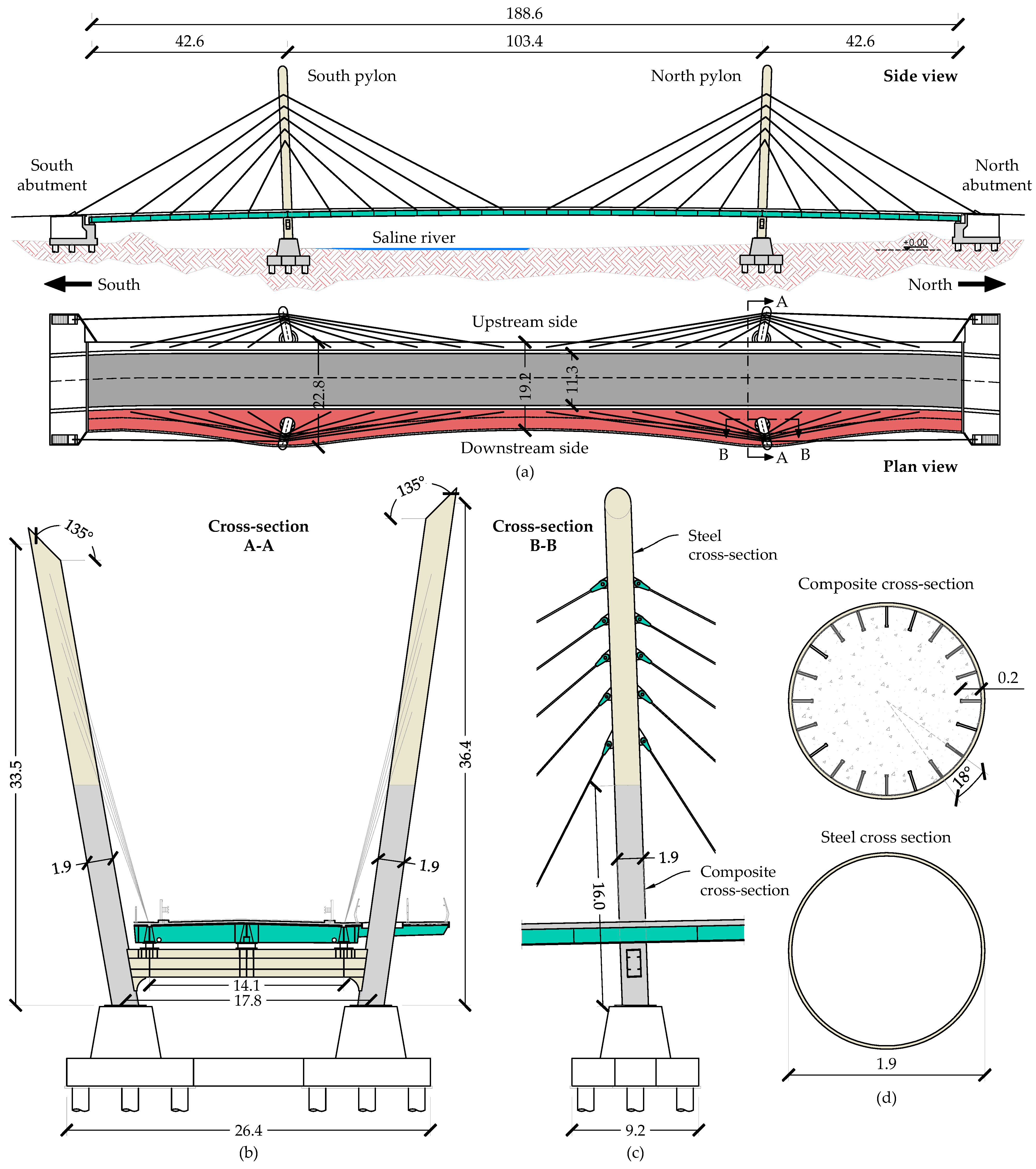
The Filomena Delli Castelli bridge is a steel-concrete composite cable-stayed bridge with three spans of 42.6, 103.4, and 42.6 m, for a total bridge length of 188.6 m. The bridge allows the road and cycle-pedestrian connection between the municipalities of Montesilvano and Città Sant’Angelo (in Central Italy) by crossing the Saline River (Figure 1). The overall deck width varies between 19.2 m and 22.8 m and includes a 11.5 m wide carriageway, two 0.75 m wide curbs to accommodate barriers, two technical paths for the stay connections, and a cycle-pedestrian path of variable width (Figure 2a).

The deck structure is constituted of two 1.2 m high I-shaped girders that are connected by I-shaped cross-beams with variable heights ranging between 0.8 and 1.2 m, and by a 25 cm thick concrete slab. The cross-beams have cantilevers that extend for a length of 1.1 m on the upstream side of the bridge, while they vary between 4.0 and 7.6 m on the downstream side. The cross-beams are 4.3 m spaced along the longitudinal direction in the lateral spans, and 4.7 m spaced in the central span. The concrete slab is connected to the main girders and cross-beams by Nelson studs and it is casted using 7 cm thick precast predalles, lightened with expanded polystyrene blocks in correspondence of the cycle-pedestrian path.

The pylons consist of four inclined steel tubes with diameter of 1.9 m and height of 33.45 m on the upstream side and 36.4 m on the downstream side, respectively (Figure 2b), filled with concrete for the first 16 m on the bottom part, and transversally connected by a 1 m wide and 2 m high steel box-girder (Figure 2b). The pylons are anchored at the base by means of 20 5.5 m long Dywidag steel bars having diameter of 40 mm, and by four shear keys that are embedded into a truncated cone-shaped concrete shaft. The foundation of each couple of pylons consists of 2 m thick and 9.2 m large square concrete plates that are transversally connected to each other by a 3 m wide and 2 m high tie beam. Each pylon basement is founded on nine 35 m long drilled piles with diameter of 1.2 m.

Stay cables are realized with bundle of 19, 25, 30, and 37 waxed and biplated parallel strands with seven galvanized wires that are made of low relaxation harmonic steel, and they are protected by a high-density polyethylene sheath. The stays are anchored to the pylons by means of forks and pin connections that are arranged on five levels at a distance of about 2.5 m from each other (Figure 2c), while, on the other side, they are equipped with adjustable anchorages that are connected to the deck by means of ribbed plates that are directly welded to the main girder webs. The two pairs of external stays spread outwards, passing from 14.1 to 26.1 m of transverse distance, to anchor to the abutment wing walls by means of 7 m long Dywidag bars having diameter of 40 mm, thus ensuring a reduction of the transverse bending in the pylons.

The abutments have a total height of about 5 m above the ground. The front walls are 1.9 m thick, while the back walls, set back of 2.25 m from the front walls, have thickness of 0.5 m. The side walls, which are connected to the frontal walls with 34.2° inclined sections, consist of 5.85 m long walls with a thickness of 3 m, on which the outermost stays of the pylons are anchored through an inclined projection. The abutment foundations are constituted by 16 drilled piles with diameter of 1.2 m arranged in three transversal rows and the cap has an almost rectangular shape of dimensions 10.3 × 16.3 m, with thickness of 1.4 m. Multidirectional negative-load pot bearings are adopted for the supports of the main girders. Lead rubber bearings (LBRs) are located at the two pylon cross-beams in the middle position. The latter control the horizontal displacements of the deck and ensure the seismic protection of the bridge through the isolation technique, by adding benefits of the period elongation to those of the energy dissipation. For construction issues, the isolators are divided into four elements, each one with a lead core; the maximum design horizontal displacement of the isolators is ±200 mm.

3. Testing Methodology

For the final proof test of the bridge before the opening to traffic, conducted on 12 October 2019, both static and dynamic tests were performed. The static load tests were executed to analyze the bridge response to traffic loads mainly in terms of deck deflections, bearing displacements and forces on stays, whereas the dynamic tests were performed to identify the modal parameters of the bridge during both the loaded and unloaded bridge conditions.

3.1. Static Proof Test

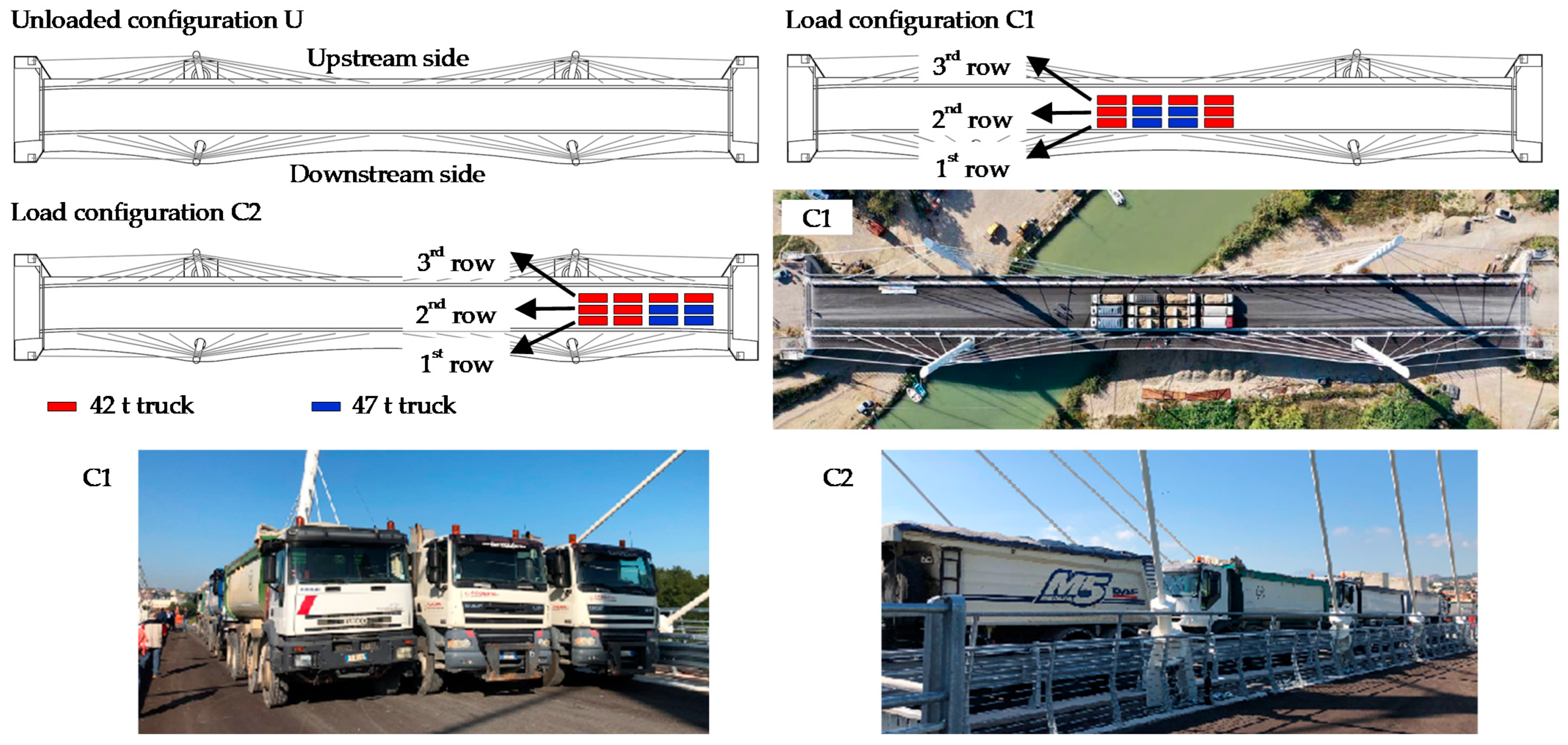
The load tests were planned to achieve the maximum design bending moments for the characteristic combination (SLS) in the most stressed cross-sections of the deck. In detail, together with the unloaded condition (U), two load configurations (C1 and C2) were adopted in order to get the maximum positive bending moments in the mid and lateral spans (Figure 3). Each configuration foresees the use of 12 fully loaded trucks that are distributed over three rows; each truck has a medium weight of about 42 t and 4 of the middle trucks of the first 2 rows (highlighted in blue in Figure 3), were also loaded with 2 additional concrete blocks per truck having dimensions of 1 × 1 × 1 m (corresponding to a load increment of about 5 t per truck). The static loads were applied through a stepped procedure in order to control the evolution of the bridge response, and to check any possible deviations from the linear behavior. The adopted loading phases (L#) are reported in

Table 1. Loading application phases.

Phase	Description	Phase	Description
L1	Unloaded bridge—U0	L7	1st truck row (4 trucks)—C2
L2	1st truck row (4 trucks)—C1	L8	2nd truck row (8 trucks)—C2
L3	2nd truck row (8 trucks)—C1	L9	3rd truck row (12 trucks)—C2
L4	3rd truck row (12 trucks)—C1	L10	Same as L9, after 1 h
L5	Same as L4, after 1 h	L11	Unloaded bridge after C2—U2
L6	Unloaded bridge after C1—U1

.

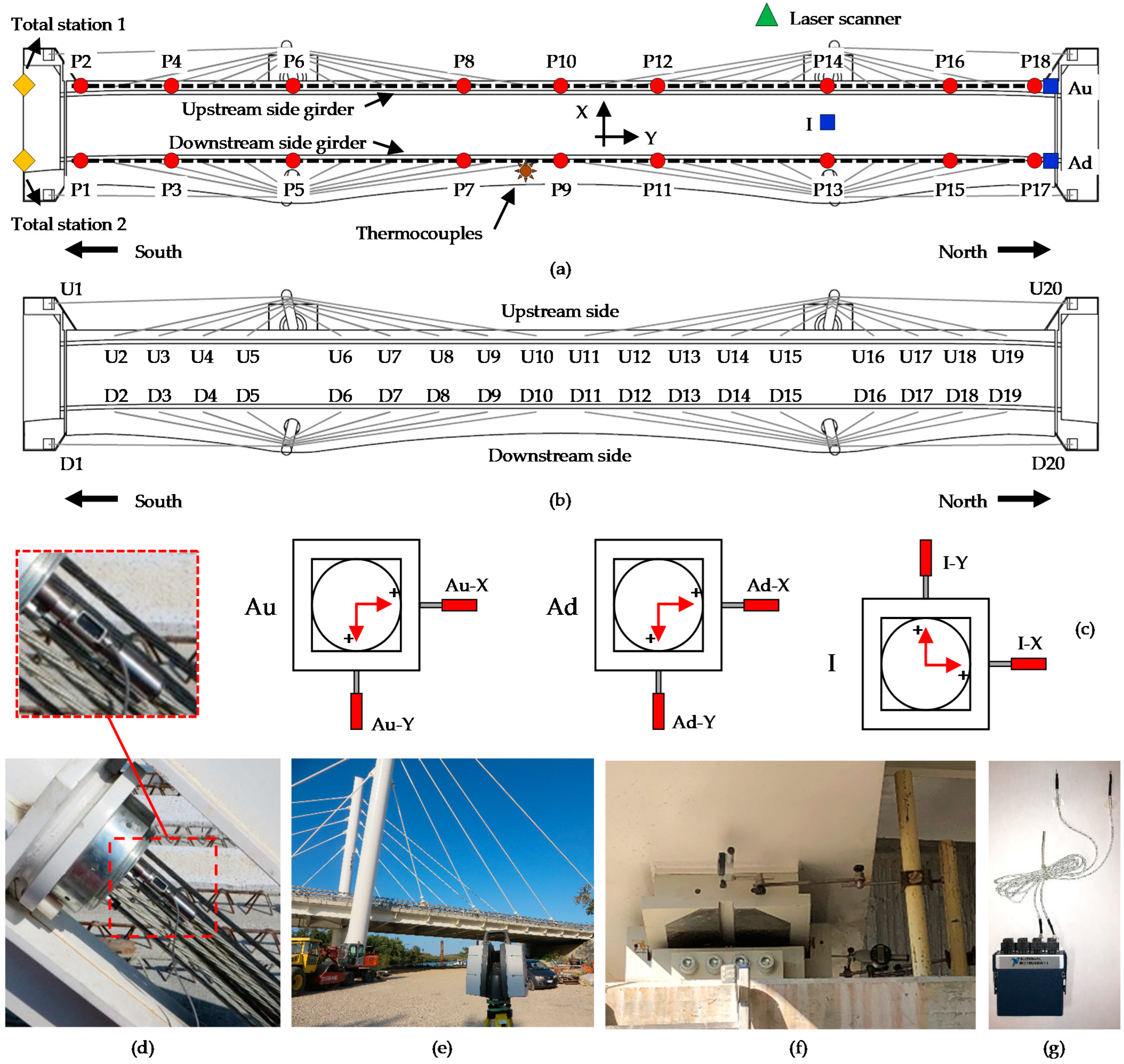
During the different phases of the load tests, the following quantities were measured (Figure 4):

• Deflections of the main girders in 18 points (P1–P18 defined in Figure 4a) that were placed along the whole length of the girders (9 points per girder), through 2 Trimble Total Stations 5600 Dr 200+ series that were positioned on the upstream and downstream side, respectively, in proximity of the south abutment;
• The axial load of the stay-cable strands, through a mono-strand load cell (maximum measurable load equal to 150 kN, Figure 4d) that was permanently mounted on a strand of each stay, and a portable analog load reader. The stays were labelled with letter D for the downstream side and U for the upstream side, and they were numbered from south to north (as reported in Figure 4b);

• Spatial displacements of the pylons, through a Leica P40 Laser scanner that was placed in a fixed position in the right bank on the upstream side (Figure 4e);
• Horizontal displacements of the 2 north abutment bearings (Au for the upstream side and Ad for the downstream side girder) and of the isolator (I) that was placed in correspondence of the north pylons, through 6 Mitutoyo digital gauges model ID-C1050B (2 per support), measuring in the longitudinal (Y) and transverse (X) directions of the deck (Figure 4c,f);
• The air and road surface temperature, through k-type thermocouples that were connected by cables to a 4-channel NI 9219 acquisition module (Figure 4g).

3.2. Dynamic Proof Tests

The dynamic characterization of the whole bridge was obtained through ambient vibration tests (AVTs) that were performed during all the proof load test phases as previously described (Table 1). The AVT measured the vibrations on the investigated bridge that were produced by the so-called ambient noise. For the case at hand, the excitation sources were mainly due to ground microtremors and wind, with the bridge close to traffic during the proof tests. Probably, some ambient noise was also produced by the nearby railway and roads, which were located almost 50 m from the bridge. Each AVT consisted of 15 min-long acceleration records that were sampled at 2048 Hz; AVTs started at 8:15 a.m. and finished at 2:30 p.m., so 25 AVTs were performed during the whole proof test day. Among the static tests, 5 main loading phases can be recognized and hence 5 main dynamic tests (Dyn.1–Dyn.5) can be individuated, as shown in

Table 2. Main AVTs that were performed during the loading phases.

Time	Dynamic Test	Loading Phase	Load Configuration
8:15–8:30 a.m.	Dyn.1	L1	U0
8:30–10:00 a.m.	---	L2 to L4	U to C1
10:00–11:15 a.m.	Dyn.2	L5	C1
11:15–12:00 a.m.	Dyn.3	L6	U1
12:00 a.m.–12:30 p.m.	---	L7 to L9	U to C2
12:30–1:45 p.m.	Dyn.4	L10	C2
1:45–2:15 p.m.	---	L10 to L11	C2 to U
2:15–2:30 p.m.	Dyn.5	L11	U2

.

Test Dyn.1 was used to capture the modal parameters of the whole bridge (in terms of natural frequencies, damping ratios, and mode shapes) at unloaded conditions (configuration U). Tests Dyn.2 and Dyn.4 were used to investigate the changes in the bridge dynamics due to the maximum applied load (configurations C1 and C2). Tests Dyn.3 and Dyn.5, in absence of load, were performed to detect the possible variations of the structural behavior with respect to the initial unloaded configuration (Dyn.1).

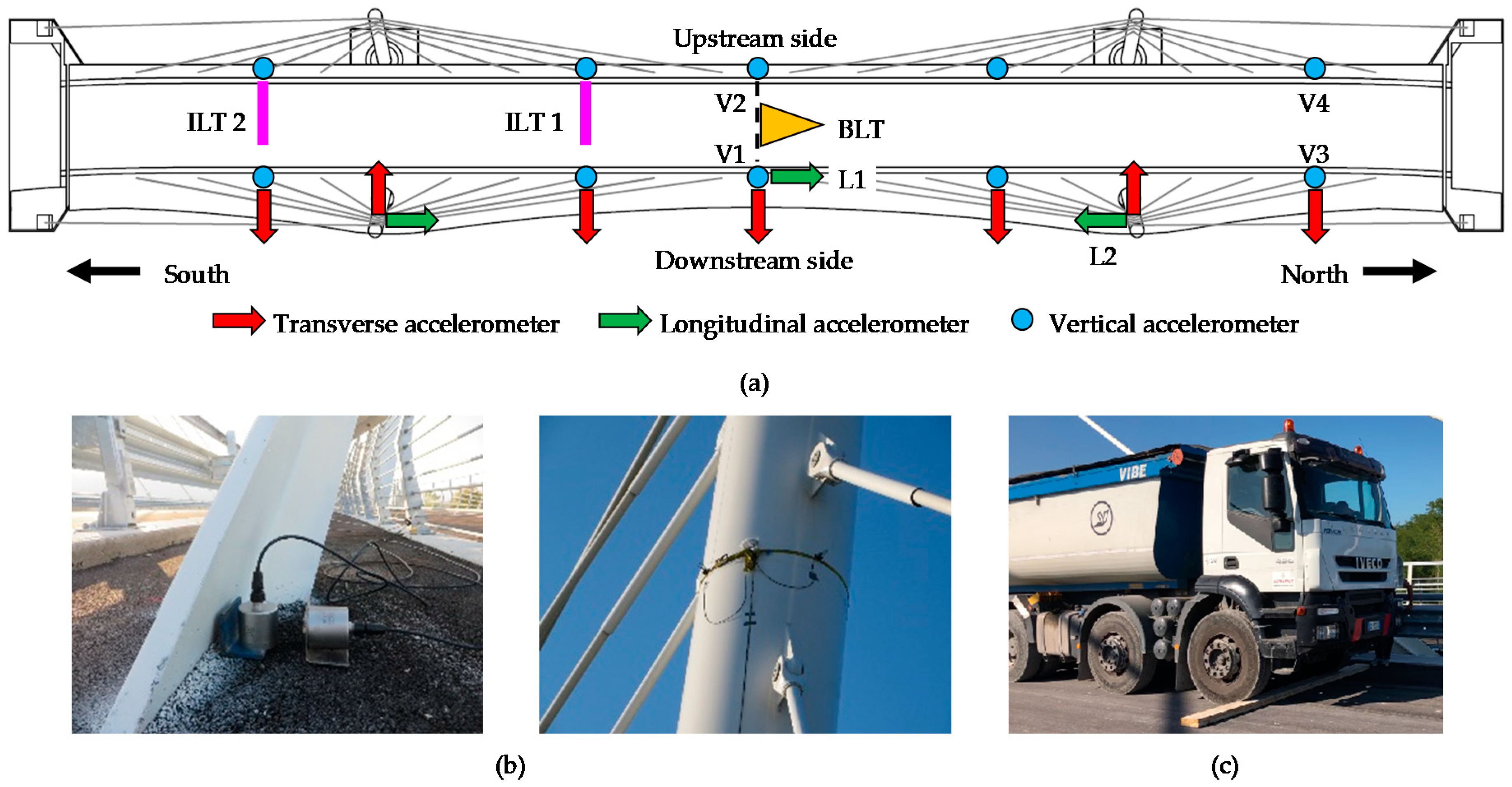
For the vibration measurements, PCB- and B&K-type piezoelectric uniaxial accelerometers with high sensitivity and low noise were used (Figure 5b). The sensors were connected by means of coaxial cables to both 4-channels NI 9234 and 3-channels NI 9230 acquisition modules that were mounted on an 8-slot NI cDAQ 9178 control unit that allowed a synchronous acquisition of signals. A laptop that was equipped with a dedicated LabVIEW software was also adopted to manage activities and to store data.

Only one sensor configuration was adopted for all AVTs, placing 20 accelerometers throughout the bridge: 16 sensors were positioned above the deck and 4 fixed to the two downstream pylons at the level of the lower stay-cable anchorages (Figure 5a). The high number of sensors and their layout allowed the identification of the global dynamics of the bridge with a good accuracy.

A further investigation of the dynamic parameters was obtained through impact load tests (ILTs) and braking load tests (BLTs), in which vibrations of much higher amplitude than those that were induced by the ambient noise were measured. ILTs were performed by adopting a fully loaded truck passing over an artificial bump (Figure 5c); two bump positions were adopted (one in the mid-span, ILT 1, and one in the south lateral span, ILT 2, as shown in Figure 5a) in order to energize as many vibration modes as possible. It is worth observing that the bump was always positioned on the upstream side of the carriageway in order to excite both bending and torsional modes of the deck. ILTs were performed in two different ways: firstly, the truck passed slowly with each axis over the bump, secondly, the truck passed the bump with a constant and relatively high speed. BLTs, which were able to induce longitudinal vibrations of the deck, were executed through the same fully loaded truck that was used for ILTs, which braked on the deck approximately at mid-span (Figure 5a). During both ILTs and BLTs, the same instrumentation and layout that were adopted for AVTs and displayed in Figure 5a were used.

An additional AVT was also performed on the truck that was used for ILTs and BLTs, in order to determine the resonant frequencies of the truck in the three main orthogonal directions with the aim to check, and likely to exclude, any possible bridge-truck interaction due to the resonant frequency of the bridge and the truck very close to each other, which can induce unexpected dynamic amplifications [25,26]. The truck dynamics was measured through 3 PCB low-noise accelerometers that were positioned above the central axes of the chassis, at a height of about 1.50 m above the ground, with measurement directions in the longitudinal, transverse, and vertical directions of the truck (orthogonal to each other).

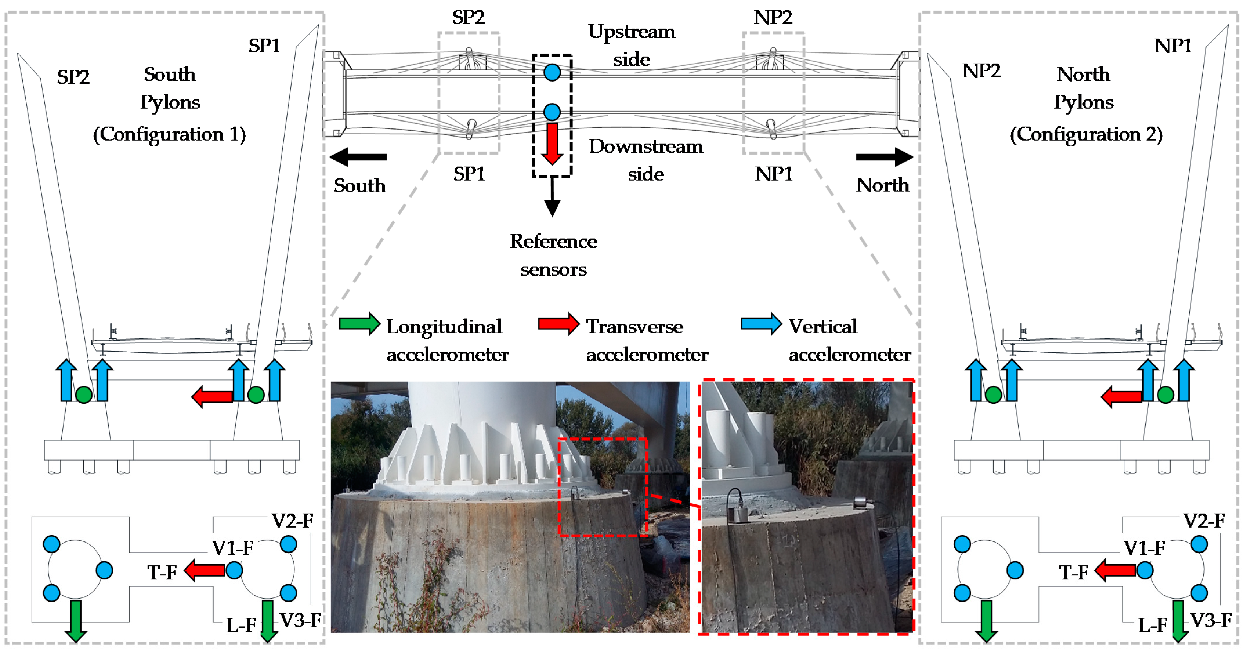
At the end of the static and dynamic proof tests, namely the unloaded condition (U2), AVTs were also carried out on the foundation of the 4 pylons in order to investigate the compliance of the soil-foundation system (i.e., its translational and rotational stiffness), and to evaluate its relevance in view of the subsequent interpretation of the experimental results through the numerical model of the bridge. As shown in Figure 6, two sensor configurations were adopted for this purpose, one for the foundation of the south pylons (SP#) and the other one for the foundation of the north pylons (NP#).

For each pylon basement, 3 sensors were positioned to measure the vertical accelerations, in order to identify the foundation rocking, while 1 sensor was positioned to measure the accelerations along the longitudinal direction of the bridge. Finally, only for the downstream pylons (SP1 and NP1), another sensor was positioned to measure the accelerations in the transverse direction. For both measurement configurations, 3 reference sensors (highlighted in Figure 6) were placed on the deck in the same positions that were adopted for the vibration measurements during the proof test. The use of reference sensors was needed to combine the measurements on pylons and on the deck, by suitably scaling the amplitudes of the frequency contents according to well-known methods that are available in the literature [27].

4. The Bridge Finite Element Modelling

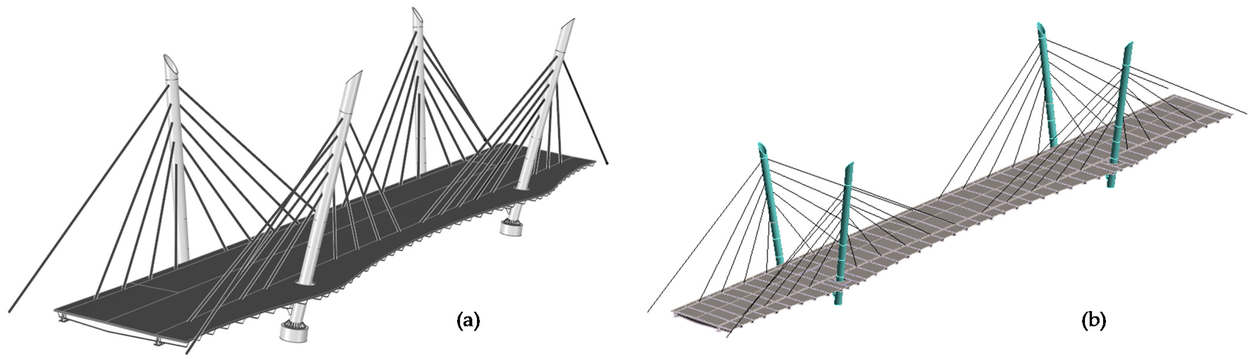
For the design of the bridge and for the proof load tests definition, a conventional 3D FE model has been developed in CSI SAP2000 environment by modelling all the structural components with beam elements. Instead, for the interpretation of the proof test results, a more refined FE model has been implemented in ANSYS, adopting shell elements for all the members in order to better capture the deck torsional behavior, which is influenced by the sectorial moment of inertia and by the warping of the cross-sections. The refined model in ANSYS was created starting from a solid model (Figure 7a), developed through the SpaceClaim software, which was then converted through the “midsurface” command into a completely shell model with surfaces of equal thickness. Finally, the correct thicknesses were assigned to all the elements and the mesh was optimized to reduce the computational effort (Figure 7b).

The two main girders and all the cross-beams were modelled with their real geometries, taking into account the presence of the relevant stiffeners (e.g., steel plates on beam webs); the concrete slab was modelled with its real thickness (25 cm) and positioned just above the steel deck structure. The slab–girders connection, which consists of Nelson studs, was modeled using elastic linear links that were calibrated to represent the elastic properties of a group of studs in their area of influence.

The relevant stiffness was obtained from the bilinearization of the shear connection nonlinear behavior that was obtained from the model that was proposed by Ollgaard et al. [28]. The pylons were modelled considering their real dimensions, inclinations with respect to the vertical alignment, and real cross-section thicknesses, which varies along the pylon height. The steel-concrete composite cross-sections of pylons (first 16 m from the foundation) were modelled adopting two shell elements, one representing the steel empty tube and the other one the concrete filling; the shell elements were rigidly connected to each other to simulate the absence of slip, exploiting the software potentials. The stays were modeled as truss elements. As for the external restraints, the pylons were assumed to be fixed at the base since tests on the foundation compliance revealed a very high translational and rotational stiffness of the soil-foundation systems, as better demonstrated and explained in the sequel.

The deck supports were modelled into two different ways, accounting for their different behavior during the static and dynamic tests. In detail, for the interpretation of the static test outcomes, it was assumed that the multidirectional negative-load pot bearings can move since frictions are overcome by the load intensity, and supports were modelled by only retaining the vertical displacements (i.e., horizontal displacements and rotations are allowed). Furthermore, isolators were modelled with elastic links that were characterized by a very high stiffness in vertical direction and by the horizontal stiffness of the real devices, obtained from the isolator manufacturer datasheet. On the contrary, for the interpretation of the dynamic tests, both isolators and bearings were modelled as fixed restraints, consistently with the very low amplitude of the ambient excitation that was not able to produce displacements on the multidirectional devices (because of friction), and only trigger the tangent stiffness of the isolators (stiffness at very low shear strains).

Similarly, also the slab concrete Young’s modulus has been varied to interpret the bridge behavior during the two different test typologies: for the interpretation of the static tests, the concrete was supposed to be cracked due to the negative bending moments as well as to shrinkage; on the contrary, for the interpretation of the dynamic tests, the concrete stiffness was not reduced, but rather increased to consider the concrete dynamic stiffness (the static elastic modulus was increased by the 20% as suggested in [29]).

The permanent loads that were relevant to the road pavement, concrete curbs, and steel barriers were also accounted for as added loads and masses. Linear elastic and modal analyses were performed for the interpretation of the static and the dynamic tests, respectively.

5. Test Results and Interpretation

In this section, the results of static and dynamic tests are presented and discussed in order to show their usefulness for controlling the bridge behavior during the loading phases. In addition, the experimental measurements are compared with the relevant numerical predictions that were obtained through the refined FE model that was previously described.

5.1. Deflections of the Main Girders

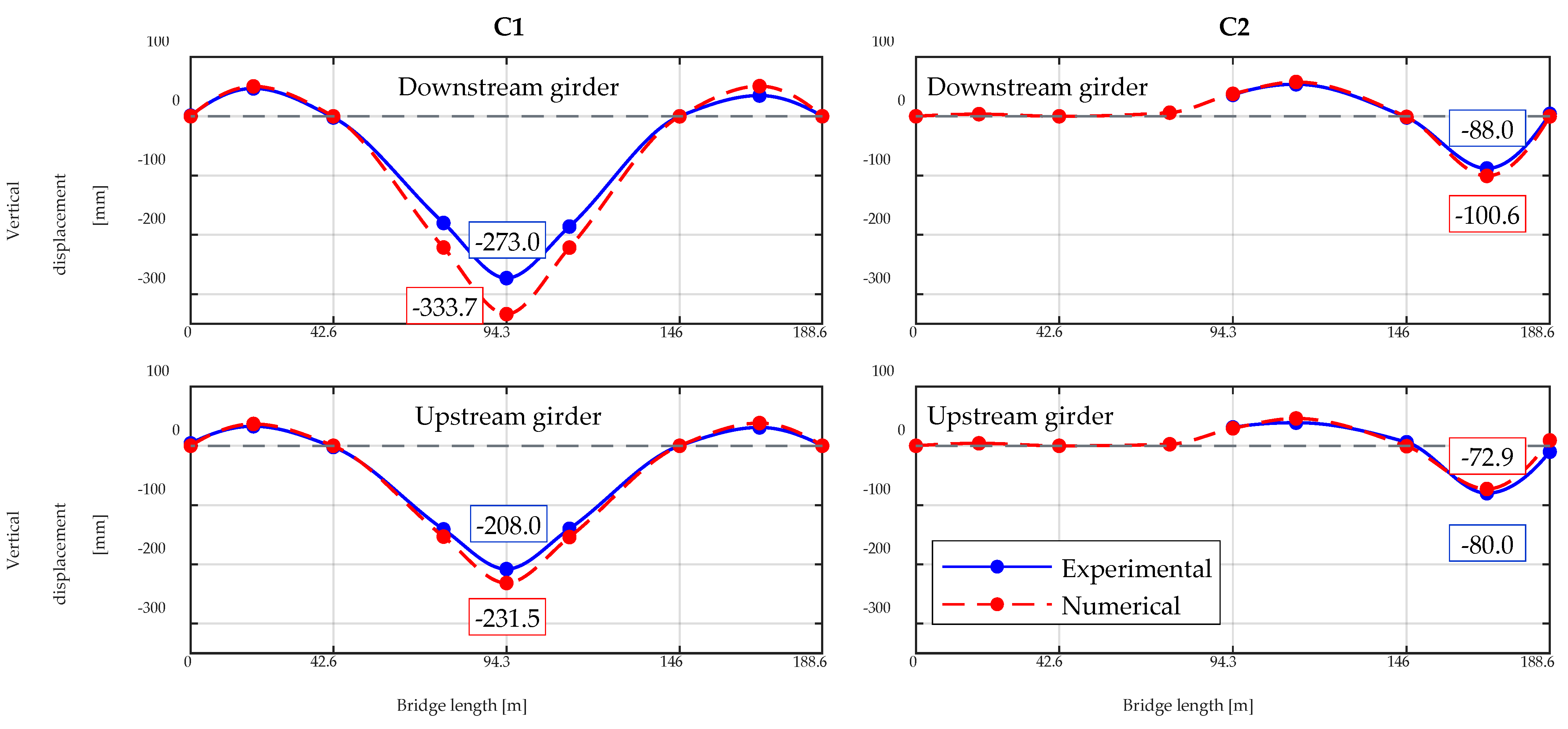
During the bridge loading phases, the vertical deflection of the deck was obtained through topographic measurements. The vertical displacements of some selected points (P1–P18) all along the girders are considered and reported in Figure 8 for the maximum loading phases (configurations C1 and C2). In detail, for C1 all the 18 points are considered and measured, whereas for C2 only those that were nearby the north lateral span (P9–P18) are taken into account since they experienced significant vertical displacements due the load position. As can be seen from Figure 8, the experimental vertical displacements of the deck vary as a function of the truck positions; for C1 the maximum experimental displacement (of about 27.3 cm) was measured at the mid-span of the bridge deck, in correspondence of the downstream side girder (the trucks are placed eccentrically in the transverse direction). On the contrary, the two lateral spans uplift of about 5 cm (4.7 cm at the mid-length of the south lateral span). As for C2, the maximum displacement of 8.8 cm was measured on the downstream side girder in correspondence of the mid-length of the north lateral span.

The experimental deflection of the main girders is compared with the numerical predictions that were obtained through the refined FE model. The comparison is also shown in Figure 8. As can be observed, the numerical displacements are in very good agreement with the experimental ones and the maximum measured deflections are slightly lower than the theoretical ones, revealing a positive outcome of the proof test.

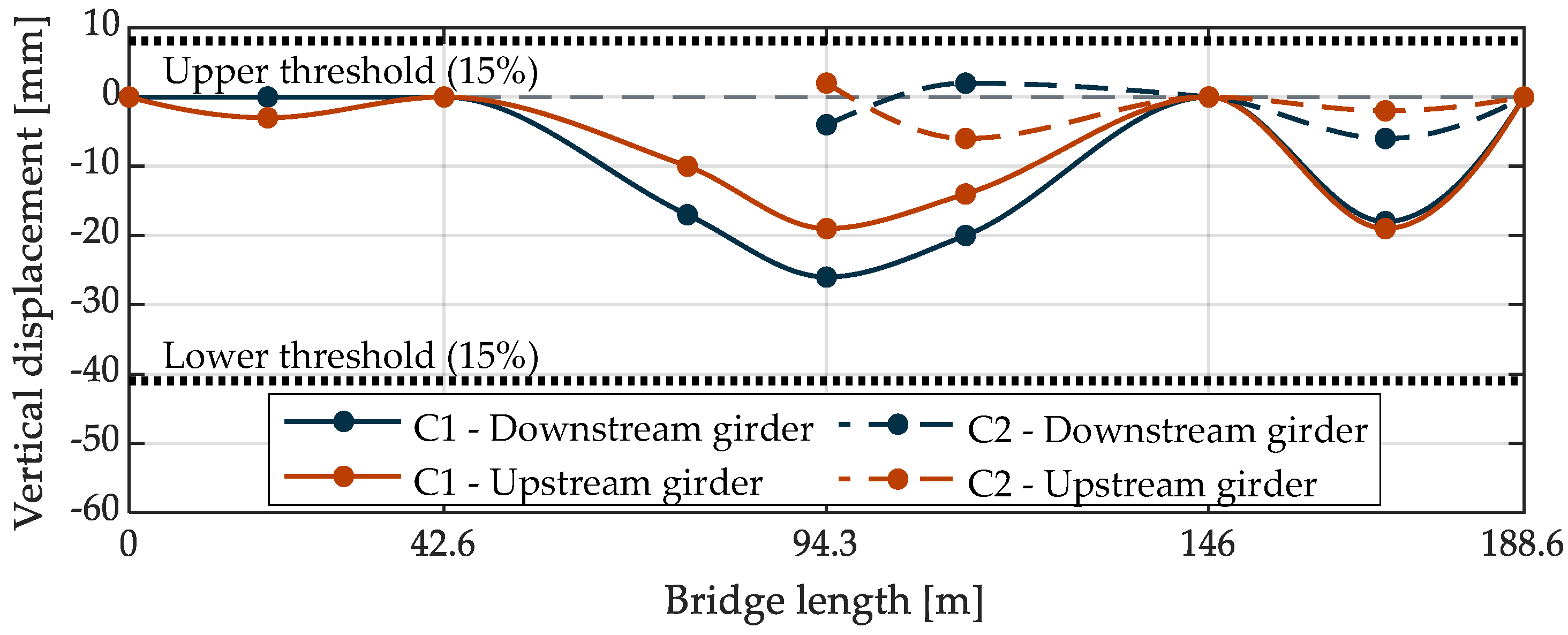
The residual deflections that were measured in the U2 configuration after the removal of loads (i.e., after C1 and after C2) are plotted in Figure 9. They are characterized by very small values, proving that the bridge almost returned to the initial configuration. Moreover, these values are largely lower than the 15% of the maximum vertical displacement that was experienced by the loaded bridge in each load configuration, as required by the Italian Standards [30] for a positive outcome of the proof test.

5.2. Axial Loads on Stays

The axial load of each stay cable during the proof load test was obtained by multiplying the axial load of the instrumented strand by the number of strands, hence assuming the load is equally distributed among each strand of the stay.

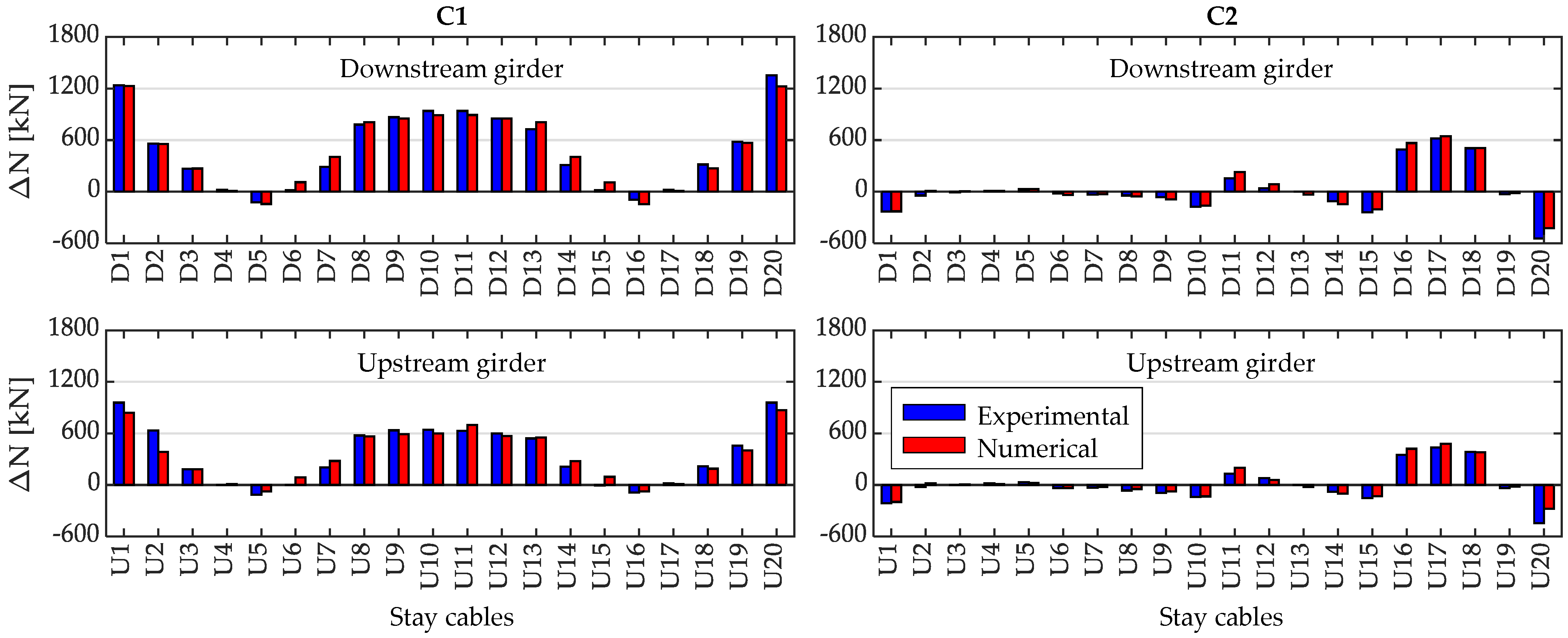
The controlled axial loads refer to the bridge in C1 and C2 load configurations and are reported in Figure 10 in terms of the axial load increase/decrease (∆N) for each stay due to the load application with respect to the unloaded condition (U₀). Negative and positive values in Figure 10 indicate decreases or increases, respectively, of the axial loads with respect to the actions due to the bridge self-weight in the unloaded condition U₀.

As can be observed, during C1 the maximum axial load increment was reached by stays on the downstream side and, in particular, in those that were placed nearby the mid-span (with the greater value just over 900 kN) and in the two stays at the lateral sides, anchored on the abutments (with values around 1200 kN). Also during C2, the axial load increment distribution on strands was consistent with the load position on the deck; indeed, in this case the maximum axial load increment was reached by stays that were placed in the north lateral span, with maximum values on the downstream side of about 600 kN.

Figure 10 also shows the comparison between the experimentally measured cable axial load increments/decrements with values that were obtained from the FE model. It is worth remarking that the FE model provides a very good estimation of the measured ∆N.

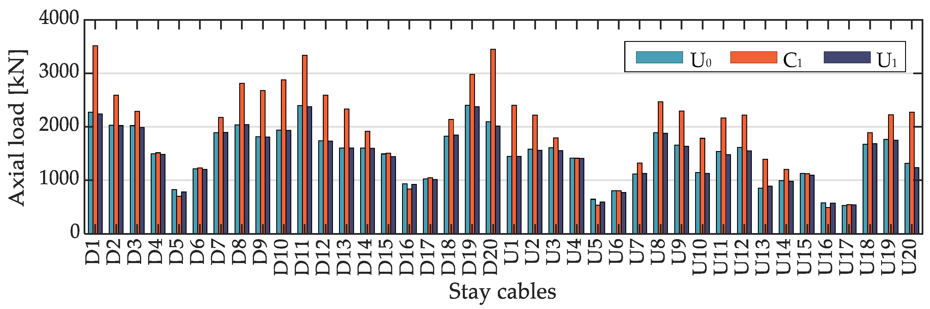
Moreover, from the measured values of the absolute forces, and the numerical applications, it was evident that all the stays remained in the elastic field. Indeed, similar values of axial loads were registered for phases U₀ (unloaded bridge before C1) and U₁ (unloaded bridge after C1), namely before and after the load test, as shown in Figure 11. Thus, it can be concluded that plastic deformations of some stays did not occur since they would have triggered a redistribution of the overall axial forces in the stays.

5.3. Displacements of Pylons

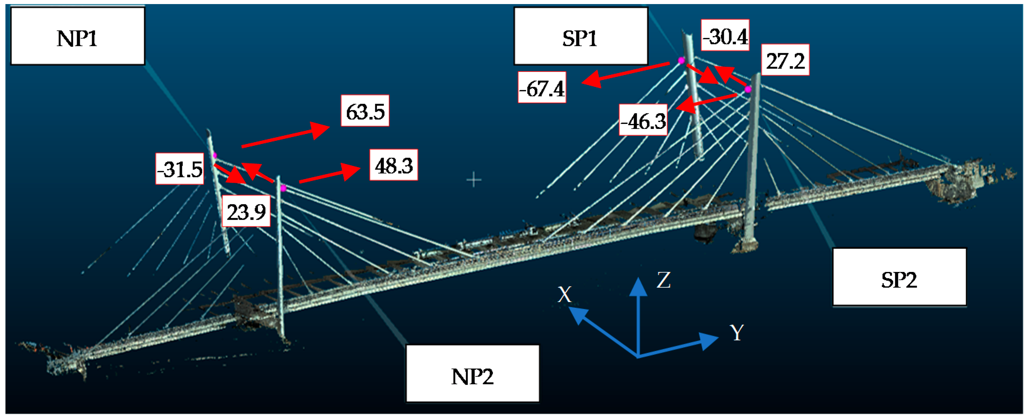
The laser scanner surveys during the proof load phases provide 3D images of the deformed shape of the overall bridge. The 3D coordinates of many points that were scattered throughout the bridge can be acquired at different loading conditions to get the well-known point clouds from which direct measurements of the bridge displacements can be obtained. The approach is promising to control the overall deformed configuration of a bridge and particularly to measure the displacements of points that are inaccessible for sensor positioning. The laser scanner acquisition was adopted to control the pylons displacements. In detail, the acquisitions were performed at unloaded conditions (phase L1) and during configuration C1, corresponding to the application of the maximum load (load phase L5), which is expected to produce the higher displacements of the mid-span deck and pylons. By comparing the acquired point clouds, the displacements that are reported in Figure 12 were obtained.

As can be observed, some parts of the bridge are absent from the cloud because they fall in shadow areas with respect to the laser scanner position. All the four pylons are well visible, hence the laser scanner acquisitions are used to analyze the pylon displacements due to loads of configuration C1. In particular, the longitudinal (Y) and transverse (X) displacements of the south and north pylons at the higher stay anchorages, labelled with SP and NP, respectively, are taken into account and reported in Figure 12. Displacements indicate that the pylons moved toward the middle of the bridge deck, both in the longitudinal and transverse directions, consistently with the applied loads (in the mid-span of the bridge on the downstream side).

The displacements of the same points that were obtained from the FE model in C1 load configuration are listed in

Table 3. Comparison between the experimental and numerical displacements of the investigated pylon points in C1 load configuration.

Point	Longitudinal Displ. (Y) [mm]		Transverse Displ. (X) [mm]
	EXP	NUM	EXP	NUM
NP1	63.5	106.5	−31.5	−26.4
NP2	48.3	77.3	23.9	19.8
SP1	−67.4	−107.3	−30.4	−26.3
SP2	−46.3	−76.0	27.2	22.0

, together with the relevant experimental ones. The reported numerical displacements are calculated by subtracting the contribution of the unload bridge self-weight from the total displacement that was obtained in C1.

It can be observed that the theoretical displacements are similar to the experimental ones, especially the transverse ones, demonstrating that the numerical model is capable of well-describing the behavior of the pylons. Moreover, the longitudinal numerical displacements are always higher than the relevant experimental ones. Finally, the longitudinal symmetric behavior of the structure is also proved, consistently with the applied loads.

5.4. Horizontal Displacements of Supports

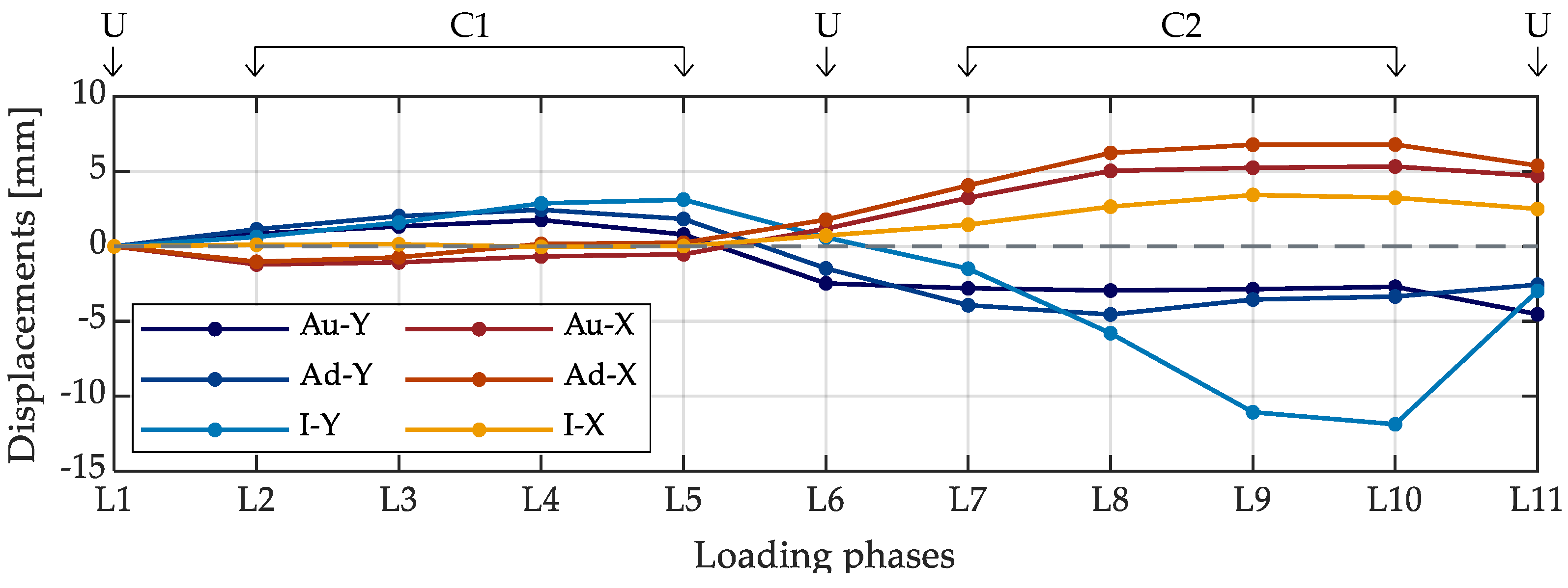
The horizontal transverse (X) and longitudinal (Y) displacements of the north abutment bearings (Au and Ad) and of the isolator (I) that was placed in correspondence of the north pylons are measured during the whole phases of the proof load test. The recorded displacements of each transducer (positioned as reported in Figure 4) are plotted in Figure 13, obtaining displacement profiles that describe the evolution of the support movements (and hence of the bridge deck) during tests.

The values of the longitudinal displacements (Au-Y, Ad-Y, and I-Y) are fully consistent with the expected rotations in the measured cross-sections of the deck because of the applied loads. Actually, in phase L5 the applied loads determine the downward deflection of the loaded central span and the uplift of the lateral spans with consistent rotations of the deck cross-sections at the supports, which are opposite in sign for the north pylon and the north abutment. Rotations of the cross-sections at the supports determine displacements at transducers that are directed towards the center of the lateral span (positive displacements). On the other hand, in phase L10 the applied load causes the downward deflection of the lateral span with consequent rotations of the deck cross-sections at the north abutment and north pylons, which determine displacements that are directed in the opposite direction with respect to the previous one (negative displacements).

The values of the transverse displacements (Au-X, Ad-X, and I-X) are almost zero for C1, while they have positive values for the load in the lateral span (C2), due to the tendency of the deck to translate downstream for the applied loads.

The higher displacements that were experienced during C2 (especially the transverse ones) are due to the position of trucks in the same lateral span where the displacements are measured. The residual displacements are almost negligible after the C1 load configuration (phase L6, with a maximum residual value around 2.5 mm) and very small after C2 (phase L11, with a maximum residual value around 5 mm). It is worth remarking that small residual displacements are physiological during tests and can be also attributable to thermal effects, which are not numerically investigated in view of the uncertainties relevant to the temperature gradient within the deck cross-section and the thermal effects on stays. Indeed, as shown in the sequel, the temperature significantly increased during the period in which the load tests were executed; consequently, a possible contribution of the thermal effects on the measured displacements, producing a deck elongation, cannot be excluded.

The developed numerical model was used to interpret the data of transducers at the supports. As an example,

Table 4. Comparison between the experimental and numerical displacements of the isolator (I).

Load Conf.	Longitudinal Displ. (Y) [mm]		Transverse Displ. (X) [mm]
	EXP	NUM	EXP	NUM
C1	3.1	4.0	0.1	2.9
C2	−11.8	−17.4	3.2	1.5

compares the measured displacements at the isolators with the corresponding numerical values; the experimental data are reproduced quite closely by the numerical model.

5.5. Air and Road Surface Temperature

The air and road surface temperatures were monitored during all the tests mainly because they may have effects on the measured dynamic parameters [31]. The air temperature recording started at 8:30 a.m. and a measure each 15 min was performed, up to 2:30 p.m. For the road surface, measures started at 9:30 and were then performed every 15 min. The trends of the air and road surface temperatures are plotted in Figure 14; it can be noticed that the air temperature uniformly increased during all the test periods, starting from 13 °C, in the early morning, up to almost 30 °C, at the end of tests. As previously stated, in view of the temperature variation, some thermal effects on the displacement measurement cannot be excluded. On the contrary, the effects of temperature on the dynamic measures were revealed to be almost negligible for the case study at hand.

5.6. Modal Parameters of the Bridge Superstructure

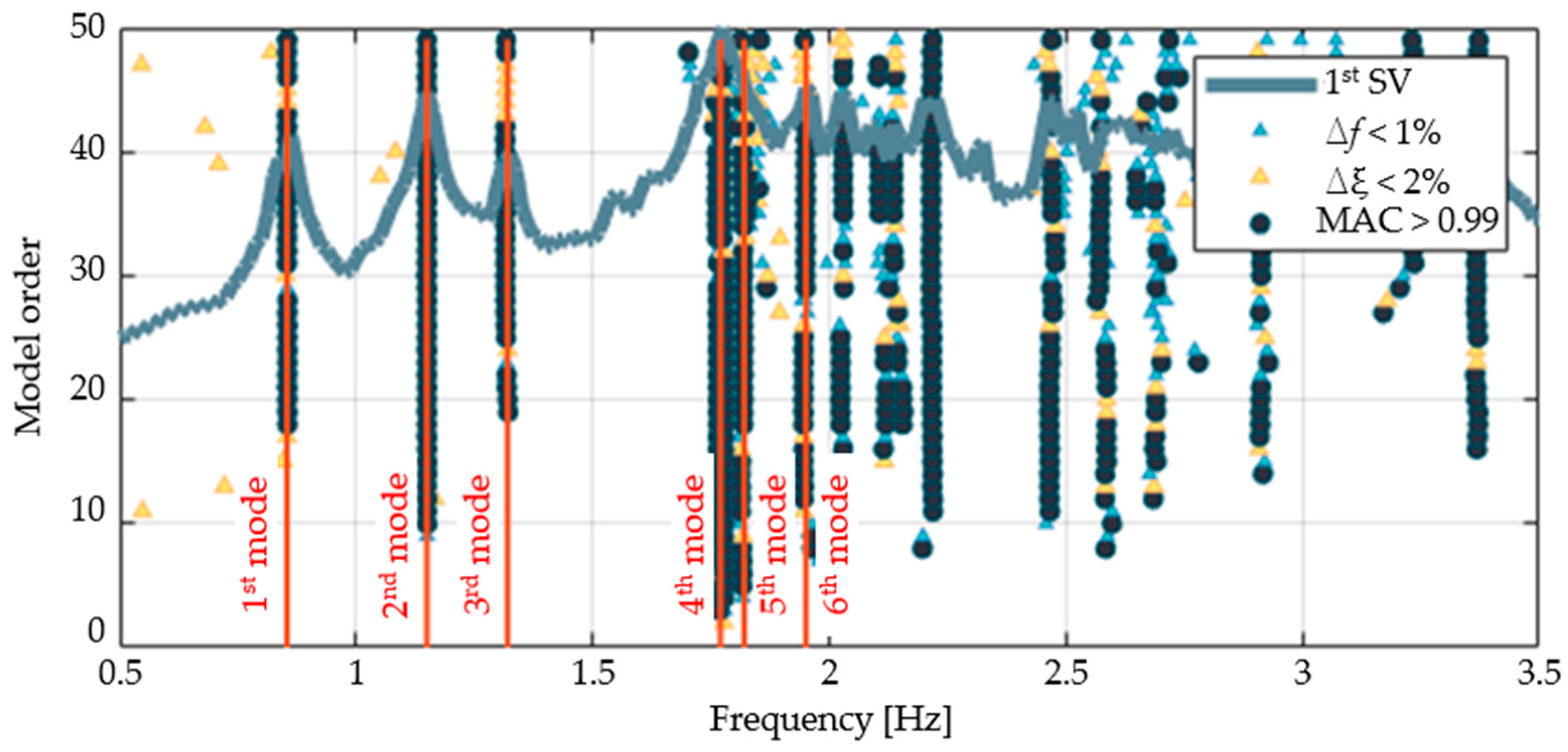
The modal parameters of the bridge are identified for all the performed AVTs (25 tests) and on the basis of the acceleration measurements, adopting the covariance-driven stochastic subspace identification (SSI-COV) technique [32]. The latter is an output-only identification method working in the time domain that assumes the excitation sources are characterized by a flat spectrum (i.e., the input is considered as a white noise). Each of the 25 performed identification procedures foresees the use of a stabilization diagram through which modes are identified once they are recognized to be stable. In this work, a vibration mode is assumed to be stable if the frequency variation (∆f) between two subsequent model orders is less than 1%, the damping ratio variation (∆ξ) is less than 2%, and the modal assurance criterion (MAC) is greater than 0.99. The stabilization diagram of the Dyn.1 test is reported in Figure 15; the first singular value (SV) is also reported for completeness and to highlight the peaks that characterize each vibration mode of the unloaded bridge.

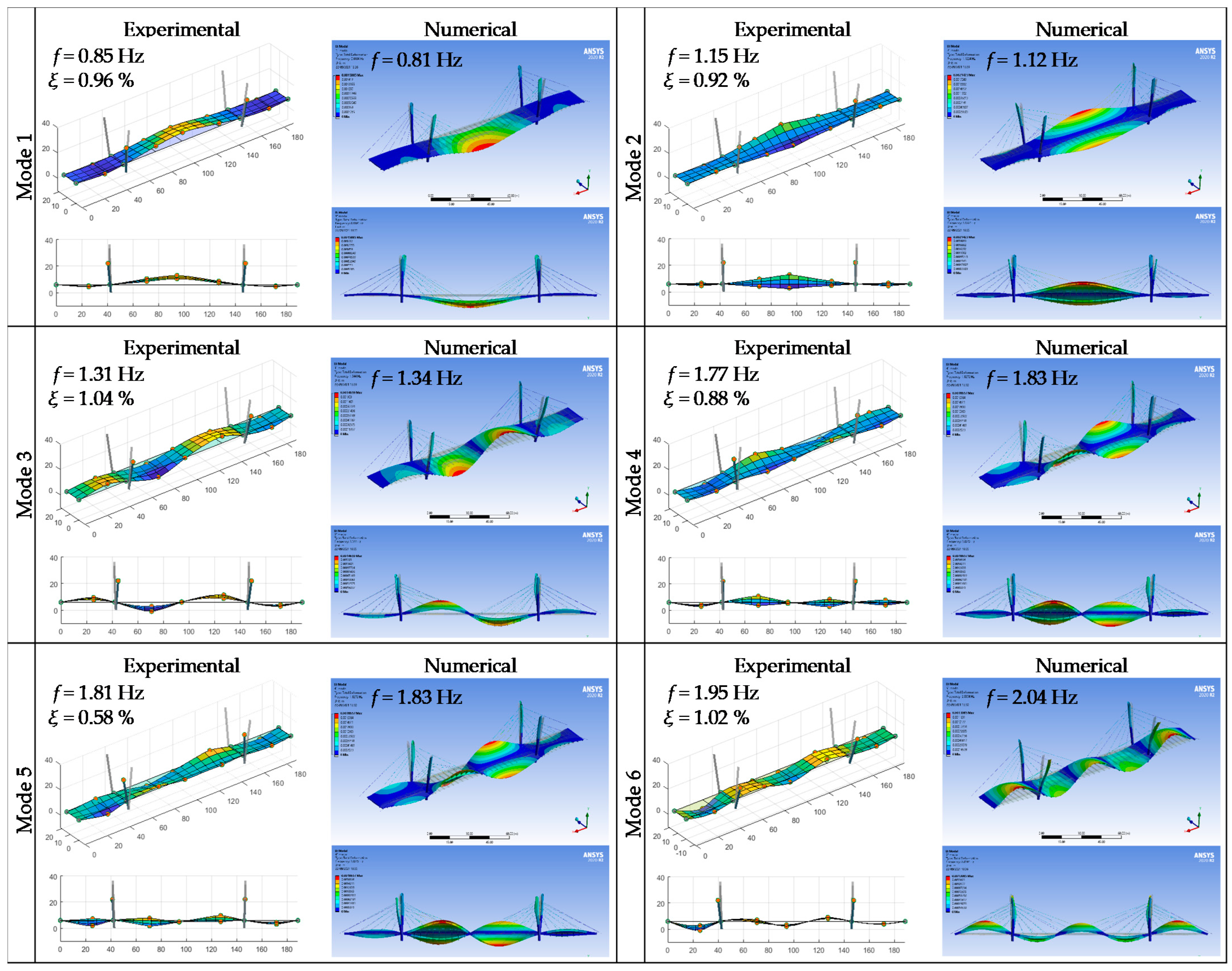
The results of the Dyn.1 test (relevant to the unloaded bridge) are taken as reference for the interpretation of the dynamic test outcomes. In Figure 16, the first six vibration modes that were identified for the unloaded bridge are reported, together with the relevant resonant frequencies and damping ratios. The first three modes represent the first bending, the first torsional, and the second bending mode of the deck, respectively. The fourth and fifth modes are both typical of the second deck torsional mode, even if the mode shapes are also characterized by a significant bending of the edge spans that, in turn, governs the response of the lateral spans more than the torsion.

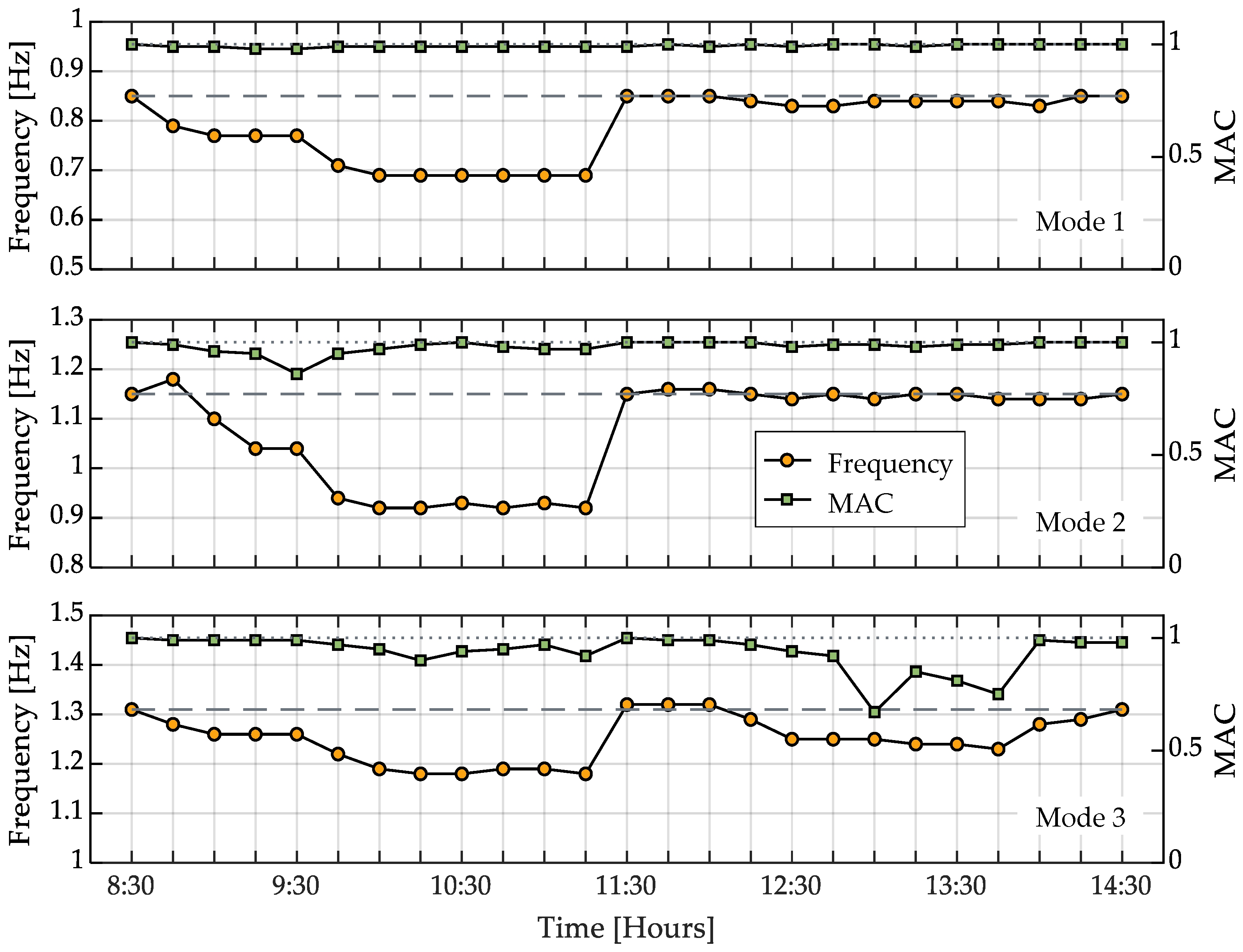
Finally, the sixth mode is the typical third bending deck mode. Figure 17 shows the evolutions of the frequency values and mode shapes (the latter expressed through the MAC indexes that were evaluated with respect to the unloaded configuration) for the first three vibration modes during the whole loading tests, which foresees a cyclic loading and unloading of the bridge. Moreover, in

Table 5. Evolution of the experimental frequencies and damping ratios during the main phases of the proof load test.

Mode	Dyn.1		Dyn.2		Dyn.3		Dyn.4		Dyn.5
	f [Hz]	ξ [%]	f [Hz]	ξ [%]	f [Hz]	ξ [%]	f [Hz]	ξ [%]	f [Hz]	ξ [%]
1	0.85	0.96	0.69	1.16	0.85	1.45	0.84	1.54	0.85	1.76
2	1.15	0.92	0.91	1.68	1.15	1.15	1.15	1.03	1.14	1.01
3	1.31	1.04	1.19	1.32	1.32	1.41	1.24	1.27	1.29	2.62
4	1.77	0.88	1.76	1.36	1.75	1.32	1.76	0.79	1.71	2.57
5	1.81	0.58	1.77	4.55	1.79	2.70	1.78	0.86	1.75	1.17
6	1.95	1.02	1.95	0.59	1.96	0.90	1.92	0.67	1.92	1.66

, the identified resonant frequencies and damping ratios that were relevant to dynamic tests of greater interest (from Dyn.1 to Dyn.5) are listed.

The trends of modal parameters, reported in Figure 17, can be correlated with the bridge loading procedures to investigate the effects of loads (and hence masses) on the bridge dynamic response. The reference frequency value, relevant to the unloaded bridge, is identified for each mode and highlighted with a horizontal dashed line in Figure 17. By gradually loading the bridge up to the C1 loading configuration (reached around 10:00 a.m.), a decreasing frequency trend is evident. In particular, the first and second modes reached frequency values that were around 20% lower than those of the unloaded configuration, while the third frequency reduced about 9%. The frequency values remained stable up to 11.15 a.m. since the C1 load was maintained for more than 1 h. At 11.30 a.m. frequencies returned to the initial values after the removal of the C1 load, demonstrating the absence of permanent damage to the structure. A similar trend can be also noticed during C2 loading procedures and mostly for the third mode, while it was not so evident for the first and second ones. This may be explained by the different position of the added masses on the deck. Indeed, the masses in the central span contribute more to the bridge dynamics with respect to those on the lateral ones, as confirmed by mode shapes. At the end of the load tests, the frequencies of the first three modes were almost the same of those that were identified at the beginning, providing useful information on the health status of the structure after the tests.

The MAC indexes remained almost always constant and close to one, demonstrating that mode shapes were not sensibly affected by the masses that were added on the deck. Only for the third mode (during C2 loading procedures) did the MAC indexes assume lower values; however, they were always greater than 0.6, meaning that the mode shapes remained quite similar.

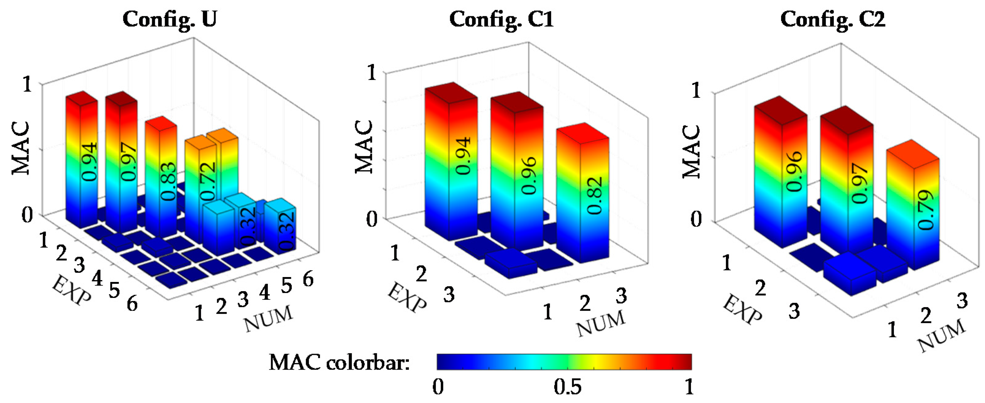
The experimental results were compared with the numerical ones that were obtained by the FE model that was described in the previous section. At first, the unloaded bridge is considered, and the numerical modal parameters, that were obtained from a classical eigenvalue analysis, show a very good agreement with the experimental ones, as can be noted from the frequency and mode shape comparisons shown in Figure 16. In particular, the first three modes show a very good agreement both in terms of frequency and mode shapes; the latter are clearly visible in Figure 18 from the MAC indexes matrix.

Finally, it is interesting to observe that the fundamental experimental frequency is slightly higher than the numerical one, revealing that the real bridge is slightly stiffer than expected, which is considered to be a positive outcome in the framework of proof testing.

As for higher modes, it must be recognized that it was not possible to properly individuate numerically the fourth and fifth experimentally-identified modes. Indeed, they are both similar to the fourth numerical model, which represents the typical second torsional mode of the deck. The latter seems to be more similar to the fifth experimental one in terms of frequency, and to the fourth experimental one in terms of MAC index. According to above considerations, the fourth and fifth experimental modes are both compared with the fourth numerical mode, and further investigations on the reason of the presented issue will be discussed in the subsequent sections, addressing the soil-foundation-superstructure possible interactions. Finally, the sixth numerical mode is quite similar to the sixth experimental ones, especially in term of frequency (difference of about 5%), whereas the mode shapes are quite different to each other, with a MAC index rather low.

The bridge numerical model was also used to interpret the frequencies that were obtained from AVTs that were performed on the loaded bridge. To this purpose, the FE model was loaded with masses that simulate the truck presence over the deck during C1 and C2 loading configurations. In these cases, the comparison between the experimental (EXP) and numerical (NUM) modal parameters was performed considering only the first three modes, which demonstrated to be the most robust ones. The frequency comparison shows a very good agreement, as demonstrated by the frequency values that are reported in

Table 6. Comparison between experimental and numerical frequencies during loading phases.

Mode	Frequency [Hz]
	U		C1		C2
	EXP	NUM	EXP	NUM	EXP	NUM
1	0.85	0.81	0.69	0.63	0.84	0.81
2	1.15	1.12	0.91	1.06	1.15	1.12
3	1.31	1.34	1.19	1.20	1.24	1.31

. Considering the fundamental frequency, also in these cases the FE model provided lower values than the experimental ones that were registered during C1 and C2. The numerical and experimental mode shapes of the first three modes are compared in terms of MAC indexes, as illustrated in Figure 18; again, a very good agreement is observed.

5.7. Results of Impact and Braking Load Tests

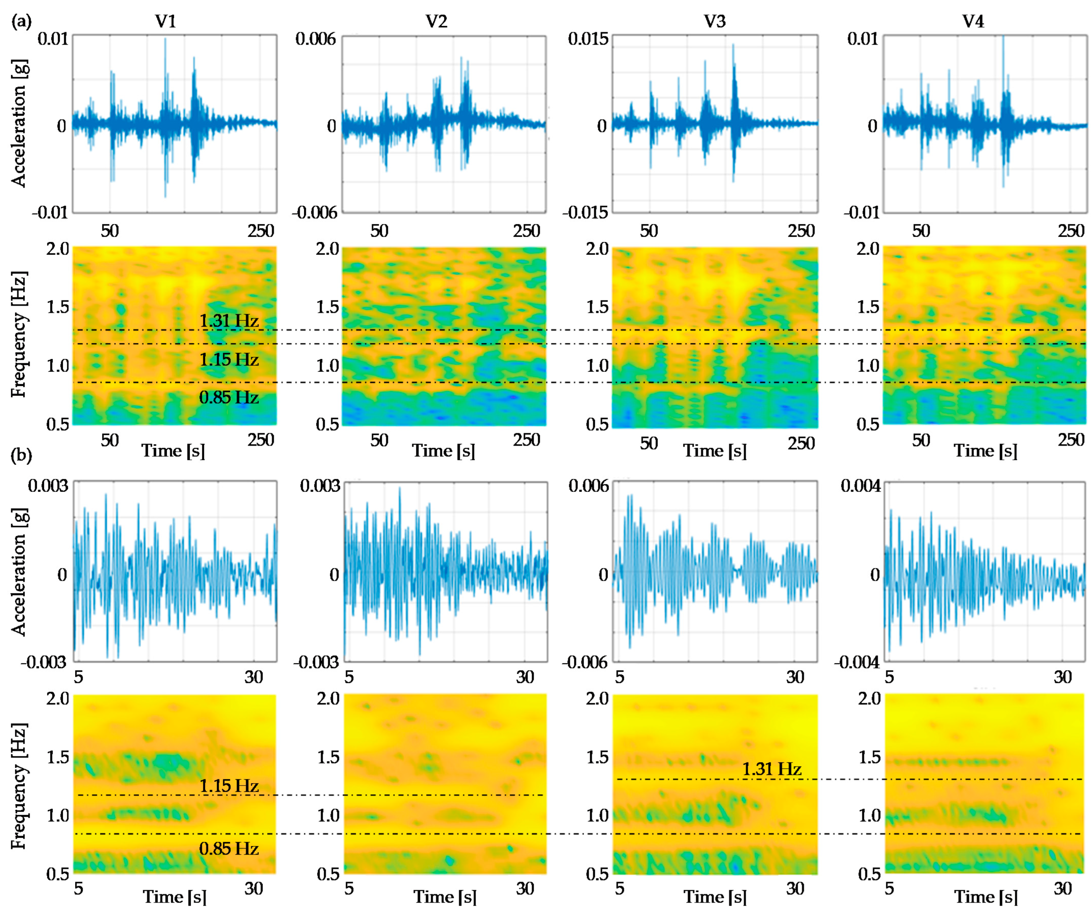
ILTs and BLTs were performed with the aim of characterizing the bridge dynamics under a higher level of vertical and horizontal excitations that were provided to the structure. Obviously, these tests are not used to identify the modal parameters of the bridge with conventional methods because the effects of the excitation that were provided to the structure quickly vanish and hence the recorded accelerations cannot be adopted neither into output-only algorithms (too short signals) nor into input-output procedures (input provided by the truck was not measured). However, they may be very useful tests for investigating the frequency dependency on the acceleration amplitude. To this purpose, the time-frequency analysis was performed in this work through the short time Fourier transform (STFT) algorithm.

The methodology provides information on the variation of the frequency content of the analyzed signals with time. Figure 19 shows the acceleration time histories and the STFT obtained from the vertical accelerations registered by accelerometers that were placed at the mid-span (V1 and V2) and at the north edge span (V3 and V4) during the truck impacts in ILT 2. As for the STFT, a light color (yellow in this work) represents the maximum frequency content of the signal, i.e., a probable resonant frequency, while a dark color (blue in this work) identifies the minimum frequency content.

From the time histories of Figure 19a, relevant to the truck passing slowly over the bump, there are four impacts that are clearly evident, corresponding to the four truck axles, and consequently, in the relevant STFTs, vertical yellow bands rapidly vanishing with time can be observed. Conversely, horizontal yellow bands are always visible in correspondence of the resonance frequencies of the bridge and remain constant over time (marked with dash-dot lines). The horizontal yellow lines (resonant frequencies) are evident considering the STFT that was obtained when the truck passes over the bump with a constant speed (Figure 19b); however, in this case, it is not easy to individuate the impact applications from the acceleration time histories. In all cases, the non-dependence of the bridge resonant frequencies on the vibration amplitude indicates a linear elastic behavior of the bridge in the observed amplitude range.

This phenomenon was observed also for ILT 1. It is worth mentioning that the accelerations recorded during the ILTs ranged between about 1.5–0.3 × 10⁻² g, values that are much greater than those that were measured during AVTs (that were of the order of about 10⁻⁴–10⁻⁵ g).

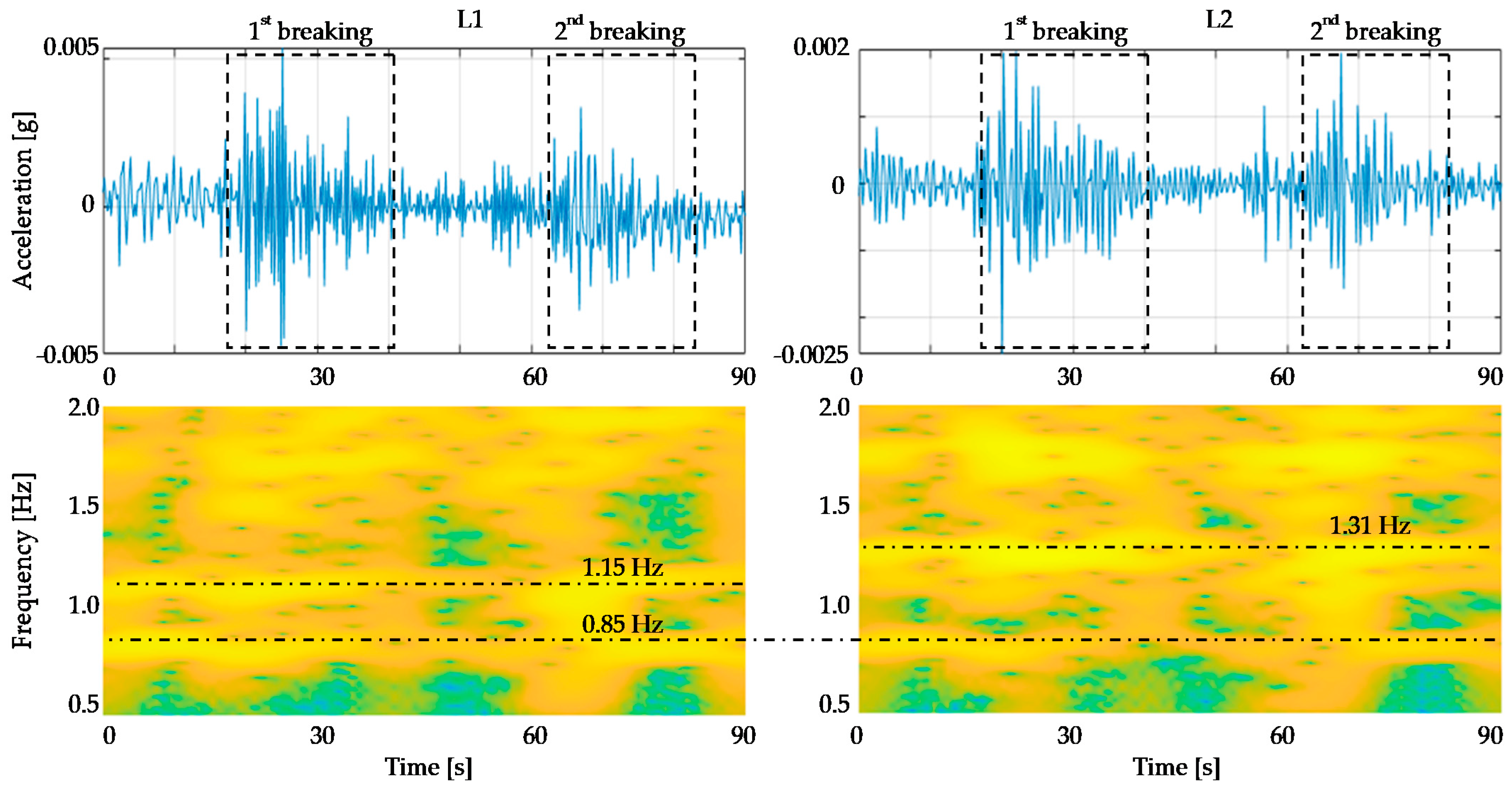
The accelerations that were recorded from BLTs can be analyzed in the same manner. In Figure 20 the time histories and the relevant STFTs for the accelerometers measuring in the longitudinal direction are reported. From the time histories, the effects of the two truck breaks, producing high oscillations of the bridge in the longitudinal direction for a time period of about 20 s, are clearly evident. The relevant STFTs reveal the typical horizontal light-yellow lines as in the case of ILTs. In detail, data from sensor L1 (placed on the bridge deck) allows the identification of the first two frequencies of the unloaded bridge (0.85 and 1.15 Hz), while that from sensor L2 (that was mounted on the downstream north pylon) permits the identification of the first and the third frequencies. As described previously, the horizontality of these lines indicates that the bridge response is elastic when subjected to accelerations due to the truck breaks; the latter are slightly lower than those experienced from the structure under truck impacts, but anyway higher than those measured during AVTs. Unfortunately, the longitudinal displacements of the deck due to the braking were not measured by the transducers that were mounted on the supports and on the isolator because the adopted sensors were not suitable for dynamic measures.

5.8. AVT on a Typical Truck

An AVT was performed on a truck that was adopted for the loading procedures and assumed to be representative for all (Figure 21). The identification aimed at investigating the truck fundamental frequencies, which are necessary to evaluate the possible bridge-truck dynamic interactions affecting the interpretation of the dynamic tests. Indeed, the trucks are usually modelled as added masses within FE models of bridges even if it is well-known that a dynamic interaction exists between the bridge and vehicles, leading to possible misunderstandings in the result interpretations, especially when the bridge and trucks have similar frequencies [25,26].

In this case, the coupled system shows the typical behavior of a tuned-mass system that is characterized by two response peaks of similar amplitudes that make the modal interpretation not easy.

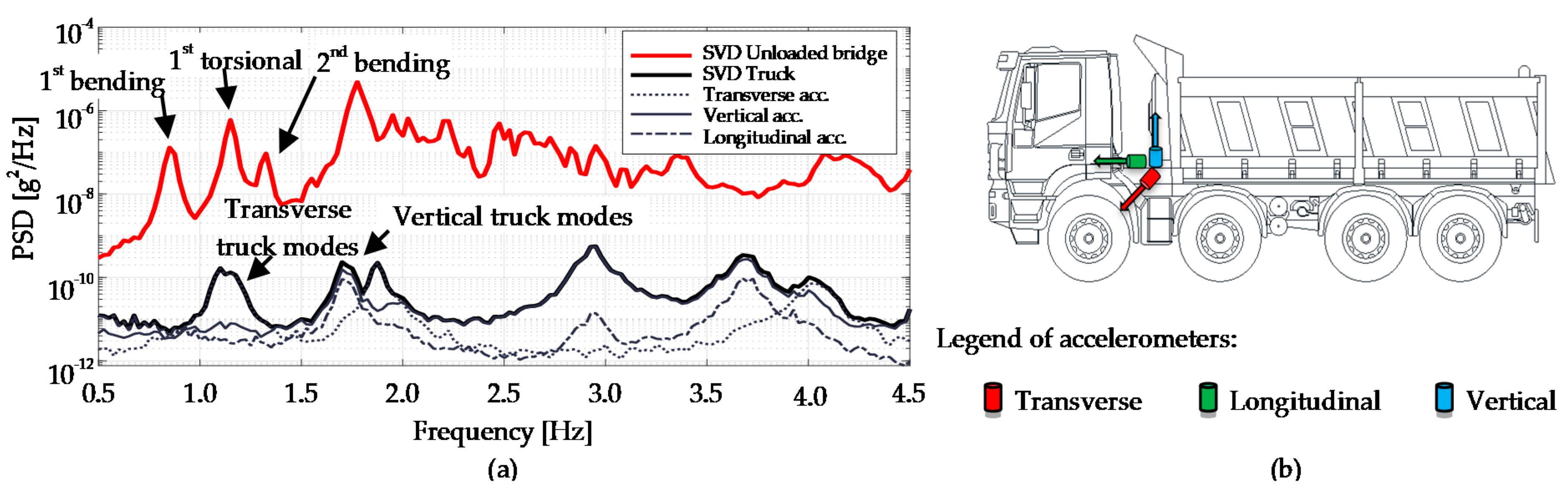
Based on the recorded accelerations on the truck, the power spectral densities (PSDs) for each of the three sensors are calculated and plotted in Figure 21a. In the PSD, which represents the frequency content of the measured accelerations, peaks highlight the presence of resonant frequencies of the system in the considered direction. In addition, the singular value decomposition (SVD) of the accelerometer recordings on the truck, and of the recording on the bridge that were made during the Dyn.1 test (unloaded bridge), are reported in Figure 21a for comparison. The transverse dynamics of the truck (represented with a dotted line in Figure 21a) is characterized by a resonant frequency of about 1.1 Hz, while the vertical and longitudinal ones (represented with continuous and a dash-dot lines, respectively) by a frequency of about 1.7 Hz. Based on previously considerations and taking into account the fundamental frequency of the unloaded bridge (0.85 Hz), it can be concluded that the vertical dynamics of trucks is characterized by different resonances and truck-bridge interaction phenomena can be excluded for the first three bridge vibration modes.

5.9. AVTs on Pylon Foundations

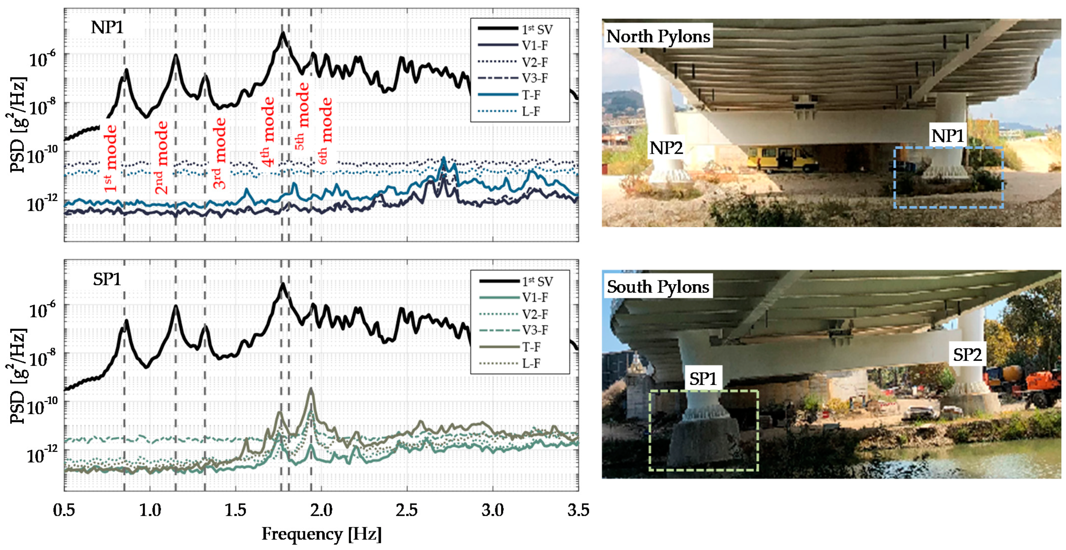
In order to provide useful information for the FE model refinement and calibration, the contribution of the soil-foundation compliance on the overall bridge dynamics is investigated, extending the measurements of vibrations to the foundation basements [33,34]. The results of the AVTs that were performed on the pylon foundations according to the configuration of Figure 6, are shown in Figure 22 in terms of frequency content of the accelerometer recordings.

In particular, the PSDs of sensors that were placed on SP1 and NP1 (V1-F, V2-F, V3-F, T-F, and L-F) are plotted together with the first SVD of the bridge deck, which summarizes the overall dynamics of the unloaded bridge. As can be seen, the higher frequency content of the foundation system is mainly detectable for frequencies that are higher than 1.5 Hz, hence the soil-foundation compliance has greater effects on the bridges higher modes, namely the fourth, fifth, and sixth, than the first three. This may partially justify problems that are encountered in the numerical interpretation of these vibration modes, considering that soil-structure interaction effects are not included in the FE model. Indeed, frequency contents are significantly different between the north and south pylons, probably due to their different restraint conditions. Actually, the downstream side antenna of the south pylon (SP1) is located within the riverbed and has a reduced backfill which gives it a higher deformability with higher peaks in the PSDs. This also affects the behavior of the whole structure for frequencies that are higher than 1.5 Hz and could explain the splitting of the second torsional mode of the deck into the fourth and fifth modes of the overall bridge.

However, the acceleration amplitudes that were recorded on the foundations are overall much lower than those that were recorded on the deck. Thus, it can be concluded that the stiffness of the soil-foundation system is so high that its deformability does not significantly affect the bridge dynamics. Consequently, the fixed base hypothesis that was adopted in the numerical model can be acceptable.

6. Conclusions

The proof testing of cable-stayed bridges cannot be reduced to a simple measure of the deck deflection that is subjected to the design loads before the opening to traffic. The testing of a complex structural system, such as a cable-stayed bridge, is a key issue even during the bridge construction, and particularly during the launching, in order to control the deck deflections and the final configuration of the pylons. The proof testing is certainly an occasion to perform a comprehensive experimental campaign on such systems with the aim of developing a digital twin model of the structure to be used in the framework of the future structural health monitoring of the bridge.

In this context, the paper presented the extensive measurement campaign that was performed during the proof testing of the Filomena Delli Castelli bridge, which combined a comprehensive dynamic experimental campaign to conventional static tests. The collected data were analyzed and interpreted to understand the behavior of the structure under different load and excitation sources. A refined finite element model of the bridge has been also developed for supporting the proof test data interpretation. This model gave good predictions on the static and dynamic responses of the bridge at unloaded and loaded conditions and its candidates to be the digital twin model for what concern the structural behavior of the bridge.

For what concerns the static bridge response, girder deflections, stay cable axial loads, pylons, and support displacements were taken under control during the whole loading phases to analyze the bridges overall response under different load conditions.

The modal parameters were monitored during all the loading procedures and their evolution has played a key role in the bridge behavior interpretation since it allowed the bridge integrity to be verified. Moreover, the impact and breaking load tests, that were performed with a truck over the deck, were useful to investigate the bridge dynamic behavior when it was subjected to higher amplitude excitation with respect to that which was provided by ambient noise.

The dynamic test that was performed on a typical truck that was used for the loading configurations allowed the exclusion of possible erroneous interpretation of the bridge dynamics due to the bridge-truck dynamic interaction phenomena. For the case at hand, the identified truck vertical modes were characterized by frequencies values that were far from the frequencies of the first bridge modes.

The dynamic tests on pylon foundations permitted the investigation of the soil-structure interaction for a better interpretation of the modal shapes of the bridge. Moreover, they were very useful to support the modelling of the bridge base restraint.

The results of all the tests were compared with those that were obtained numerically and provided by the finite element model; the latter revealed trustworthy in representing the bridge behavior when subjected to static and dynamic inputs of different amplitudes. In detail, the static displacements were well interpreted by the model and the obtained modal parameters were in very good agreement with those that were experimentally identified, both for the unloaded and then for the loaded bridge.

In conclusion, the proposed testing methodology could represent a good practice for the proof testing of cable-stayed bridges, proving that extended measurements and a refined model can lead to a good interpretation of the behavior of a complex structure and they could be a valid base for a future structural health monitoring of the bridge.