Article

Lane-Changing Strategy Based on a Novel Sliding Mode Control Approach for Connected Automated Vehicles

1
The Key Laboratory of Road and Traffic Engineering, Ministry of Education, Tongji University, Shanghai 201804, China
2
College of Transportation Engineering, Tongji University, Shanghai 201804, China
*
Author to whom correspondence should be addressed.
Appl. Sci. 2022, 12(21), 11000; https://doi.org/10.3390/app122111000
Submission received: 28 August 2022 / Revised: 16 October 2022 / Accepted: 25 October 2022 / Published: 30 October 2022

Abstract

:
Safe and efficient autonomous lane changing is a key step of connected automated vehicles (CAVs), which can greatly reduce the traffic accident rate and relieve the traffic pressure. Aiming at the requirements of the smoothness and efficiency of the lane-changing trajectory of CAVs, it is necessary to design the lane changing controller to integrate the sensing, decision-making, and control tasks in the driving process. Firstly, based on the vehicle dynamics model, this paper proposes a vehicle lane-changing control strategy based on NNTSMC method (neural network enhanced non-singular fast terminal sliding mode control). The designed lane-changing controller can well realize the designed path tracking, and both lateral position and yaw angle can well track the expected value. This method enables the vehicle to control the front wheel steering angle intelligently, and the lateral acceleration during steering changes in the small scope, which ensures the steering stability of the vehicle. In this study, an improved adaptive RBF neural network with bounded mapping is designed to estimate the upper bound of the total disturbance of the system, which effectively reduces the chattering phenomenon of the control force. The Lyapunov function constructed in this study proves that the designed controller can ensure the stability of the controlled system. Finally, a comparative experiment is performed by the MATLAB/Simulink-CarSim co-simulation. Compared with SMC and TSMC (non-singular fast terminal sliding mode control), the proposed method has a performance improvement of at least 58.0% and 34.1%, respectively. The effectiveness and superiority of the proposed control method were confirmed by the experiments on the co-simulation platform.

1. Introduction

Lane change is one of the most common maneuvers for vehicles on the road, and it needs drivers to consider risk avoidance in multiple directions at the same time, which is usually a driving behavior with high-risk coefficients. In 1999, there were more than half a million lane change-related accidents in the United States in one year [1]. Data show that, during lane changes, driver stress increases significantly, and driving is more prone to errors, leading to higher risks. Vehicle lane-changing behavior is influenced not only by the surrounding traffic environment but also by the surrounding traffic flow, hence research into autonomous lane-changing technology is crucial [2]. To accomplish autonomous lane-changing driving, vehicles can employ the vehicular networks [3] or use the on-board sensors to gather information about the surrounding traffic [4]. Furthermore, the built-in sensors can help vehicles with measuring operating conditions [5]. These devices may allow them to make more informed decisions about the lane-changing procedure, improving vehicle safety, comfort, and efficiency [6]. It is worth mentioning that related technologies related to vehicular networks and vehicle control system, such as authentication and privacy schemes, are also important guarantees for the reliable operation of vehicles [7,8,9].
The key technologies of autonomous lane change can be divided into three categories [10]: lane change decision, lane change path planning, and lane change path tracking control. A lane change decision provides a logical direction for vehicle lane shift. Currently, the most frequent lane shifting models utilized in vehicle lane-changing decision-making mechanisms are the Gipps model [11], the MITSIM model [12], the AIMSUN2 model [13], the CA model [14], the CORSIM model [15], and the SITRAS model [16]. The design of the lane change path must be taken into consideration if it is decided to perform a lane change after the judgment of lane change decision [17]. The purpose of the lane change path design is to make the vehicle have a virtual path as a reference in the process of lane change, so that the lane change action can be completed more safely and smoothly [18,19]. The planning of lane change trajectory needs to transform the time and distance planning problems into constraint optimization problems, and the evaluation indexes in the driving process need to be considered to calculate the reference trajectory satisfying the safety, comfort, and lane change efficiency [20]. The polynomial method [21], trapezoidal acceleration method [22], arc trajectory planning method [23], sine function method [24], and other trajectory functions are indeed common lane change reference trajectory design methods. Designers can choose a solution according to the characteristics of application scenarios as well as the advantages and disadvantages of each method [25].
It is necessary to investigate autonomous vehicle lane-changing to improve driving safety and road smoothness. The actual situation of a vehicle lane-changing procedure can be simplified to a straightforward lane change scenario, which includes the target vehicle A 0 , vehicle A 1 in front of the lane, and vehicle A 2 in the neighboring lane, using an urban two-lane road as an example. Figure 1 depicts the schematic diagram of a lane-changing scenario. Vehicle A 0 has lane change intention because it is dissatisfied with the current lane’s speed due to the vehicle A 1 ’s slower speed in front of it. After vehicle A 0 has the demand for a lane change, it should not have a serious impact on the traffic flow on the basis of ensuring its driving demand. Vehicle A 0 moves into the stage of preparing for a lane change in phases t 0 t 1 . Vehicle A 0 crosses the two-lane decomposition line at time t 2 in phases t 1 t 3 , which is a lane-changing operation. Phases t 1 t 3 correspond to the lane-changing process, where vehicle A 0 crosses the two-lane separation line at t 2 .
Vehicles with intelligent lane change controllers can avoid human error to the greatest extent possible, lowering the risk of collision with vehicle A 1 and vehicle A 2 on the road. The lane-changing time and trajectory can also be strictly tracked by using mathematical calculations rather than the driver’s experience judgement. Based on this process, we can conclude that the use of lane-changing technology will significantly improve CAV’s safety, lane-changing efficiency, and passenger comfort.
Aiming at the demand of lane-changing technology, this study proposes a novel lane-changing control strategy based on the NNTSMC method. The contributions of this paper are as follows: (1) The lane-changing control system oriented to the desired lane-changing trajectory is designed based on the vehicle dynamics model and road condition information. (2) A modified sliding mode control method for lane-changing is designed, which can avoid the shortcomings of traditional sliding mode control. (3) The constructed Lyapunov function demonstrates the stability of the control system. The lane-changing controller is constructed in MATLAB/Simulink-CarSim co-simulation environments. The effectiveness and superiority are confirmed by several experiments.
The remainder of this paper is logically organized as follows: Section 2 primarily analyzes the related work of lane-changing through the literature across the world. The mathematical derivation of the vehicle dynamics model is given in Section 3. The vehicle lane-changing controller description and problem formulation are covered in Section 4. Section 5 contains the analysis of the performances of the verification experiments and the effectiveness of the control mechanism. Section 6 presents a brief conclusion.

2. Related Work

The most fundamental requirement for accomplishing lane change is vehicle motion control that meets the criteria of trajectory tracking, in addition to faultless lane change judgment and vehicle trajectory planning [19]. If the vehicle trajectory tracking does not satisfy the kinematics and dynamics of the vehicle, as well as the driving limitations, the vehicle will vibrate while driving. In addition to reducing passenger comfort, driving shock creates a significant potential safety threat when driving at high speeds. In high-speed driving scenarios, the controller must meet the requirements of quick response speed, high response accuracy, and high adaptability to respond to diverse vehicle lane-changing conditions. In addition to the studies mentioned above, there are numerous other studies concentrating on the tracking of autonomous vehicles’ lane change trajectories, the most of which are based on kinematics or dynamics models and achieve tracking control using different control techniques.
In order to determine the expected yaw angle and yaw speed of vehicles changing lanes, Ren et al. [26] created the lateral acceleration based on positive and negative trapezoidal restrictions. After that, the tracking control law of the longitudinal and lateral coupling variable structure for lane change is constructed using the finite-time sliding mode approach law. Qi et al. [27] researched lane change control of intelligent vehicles employing four-wheel active steering technology to enhance the control performance of vehicle lateral movement. A standard cosine function lane change trajectory is the lane change route model. They created a Simulink simulation model for the closed-loop control system of the vehicle lane shifting path tracking and performed simulation experiments based on the fuzzy adaptive PID theory. The outcomes of the simulation demonstrate that the proposed lane change tracking controller can actually accomplish the desired lane change track tracking. Guo et al. [28] built a novel dummy variable and derived the trajectory tracking controller of a closed-loop control structure by applying integral backsliding approach in order to accomplish lane change trajectory planning and tracking in curves and increase the active safety of vehicles. The trajectory tracking controller’s closed-loop control structure is constructed, and Lyapunov theory is used to assess the stability of the suggested trajectory tracking controller. In order to solve the vehicle’s robust path-following control problem and satisfy the requirements for lateral stability, Chen et al. [29] proposed a H robust control scheme. Their proposal was made in response to the phenomenon that the delay and packet loss brought on by the network would adversely affect the stability and performance of the system. Finally, a comparison with the scenario of no delay and packet loss is used to demonstrate the usefulness of the suggested strategy. For model uncertainty and measurement noise, Li et al. [30] suggested a robust control rule to inhibit these two matching variables, built an adaptive robust controller to maximize path tracking accuracy, and demonstrated its effectiveness employing MATLAB/Simulink-Trucksim co-simulation.
In order to realize the path tracking capability under complicated road scenarios such as low friction coefficient and road disturbance, people have made unremitting efforts. A multi-point pre-view trajectory tracking technique for autonomous vehicles was proposed by Luo et al. [31]. This tracking algorithm takes into account the complexity of the sweeper’s practical application background and employs a way of combining feedforward and feedback control to regulate the vehicle’s lateral movement. The feedforward control section calculates the needed angle using the road information gained from the target trajectory’s curvature detection component, while the feedback control is corrected using the lateral deviation obtained from the trajectory deviation detection. Both the computer experiment and the real-world vehicle test produce positive findings. Chen et al. [32] suggested a path tracking method using an untraced Kalman filter to maintain path tracking performance and increase stability when driving at high speeds on low friction coefficient roads by calculating the vehicle’s critical state and road adhesion coefficient. The path tracking control is then realized using a predictive controller based on a linear time-varying model.
Most of the current research focuses on the control method, and few of them incorporate the vehicle’s dynamic mechanism model when designing lane-changing controllers. The design of the control method must consider the physical structure of the vehicle to have practical significance, which is often ignored. This paper develops a lane-changing controller based on the vehicle dynamics model and sliding mode control algorithm, allowing the controlled vehicle to achieve good lane-changing action and preset path tracking in complex traffic scenarios.

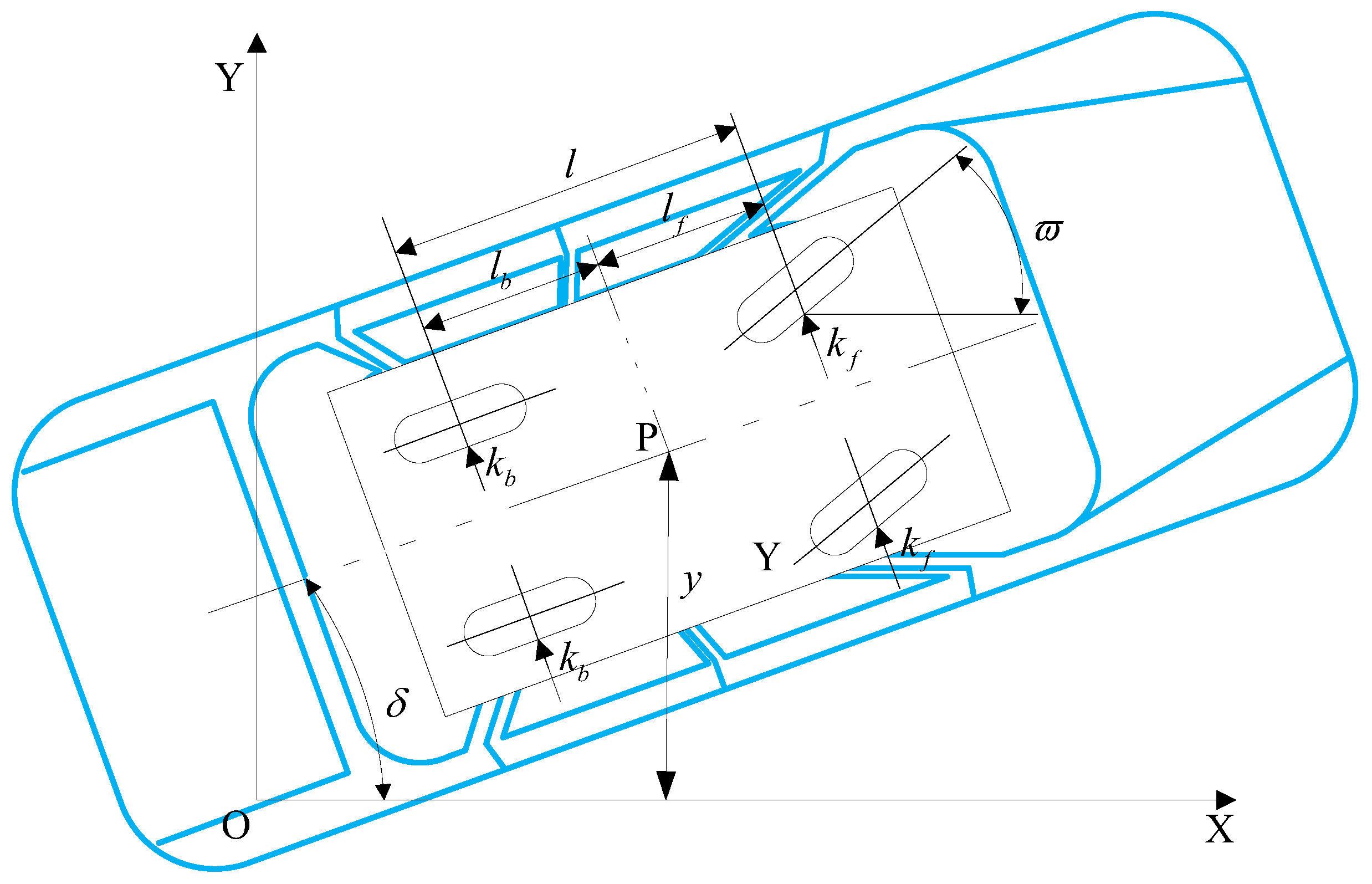
3. Vehicle Dynamics Model

In the process of lane-changing, in addition to maintaining the original longitudinal movement, the vehicle also needs to make appropriate lateral movement according to the road conditions. A schematic diagram of vehicle kinematic model is shown in Figure 2. The motion of the two dimensions is not simply superimposed. Considering generality, the dynamics model of vehicle in lane change process is modeled. In order to facilitate the problem analysis and the realization of control objectives, in the inertial coordinate system OXY , the 2-DOF vehicle dynamic equation of the vehicle is established as follows:
y ˙ y ¨ δ ˙ δ ¨ = 0 1 0 0 0 2 · k f + 2 · k b m v 2 · k f + 2 · k b m 2 · k f · l f 2 · k b · l b m v 0 0 0 1 0 2 · k f · l f + 2 · k b · l b I z v 2 · k f · l f 2 · k b · l b I z 2 · k f · l f 2 + 2 · k b · l b 2 I z v y y ˙ δ δ ˙ + 0 2 · k f m 0 2 · k f · l f I z u
where y and δ denote the lateral offset and the yaw angle of the vehicle, respectively. m is the quality of the vehicle. I z represents the moment of inertia around the vertical-axis of the vehicle. k f and k b stand for the front and rear tire cornering stiffness, respectively. l f and l b are the distance between the front and rear axles and the center of the vehicle mass, respectively. v is the longitudinal speed. y is the distances from the center of mass P of the vehicle to the x-axis. ϖ is the front wheel angle of the vehicle which is described using the controller input variable u.
The vehicle dynamic Equation (1) can be simplified by taking into account the system’s internal parameter inaccuracy and external interference. The model can be shortened to:
y ¨ δ ¨ = k 11 k 12 k 21 k 22 y ˙ δ ˙ + 0 1 0 1 y δ + 1 2 u + Δ f
where k 11 k 12 k 21 k 22 = K , 0 1 0 1 = F , 1 2 = . Simplify the definition of two of the key variables to form the expression θ = y δ .
θ ¨ = K θ ˙ + F θ + u + Δ f
= f + u + Δ f
where Δ f represents the lumped error of the system.
According to the state equation of the system, the lateral displacement, lateral velocity, yaw angle, and yaw velocity of the vehicle can be analyzed under the given input of the front wheel angle. The purpose of lateral lane change control is to reduce the deviation of the trajectory designed for tracking. It is required that the controller can analyze the deviation of the vehicle tracking at a given front wheel angle through the state equation.

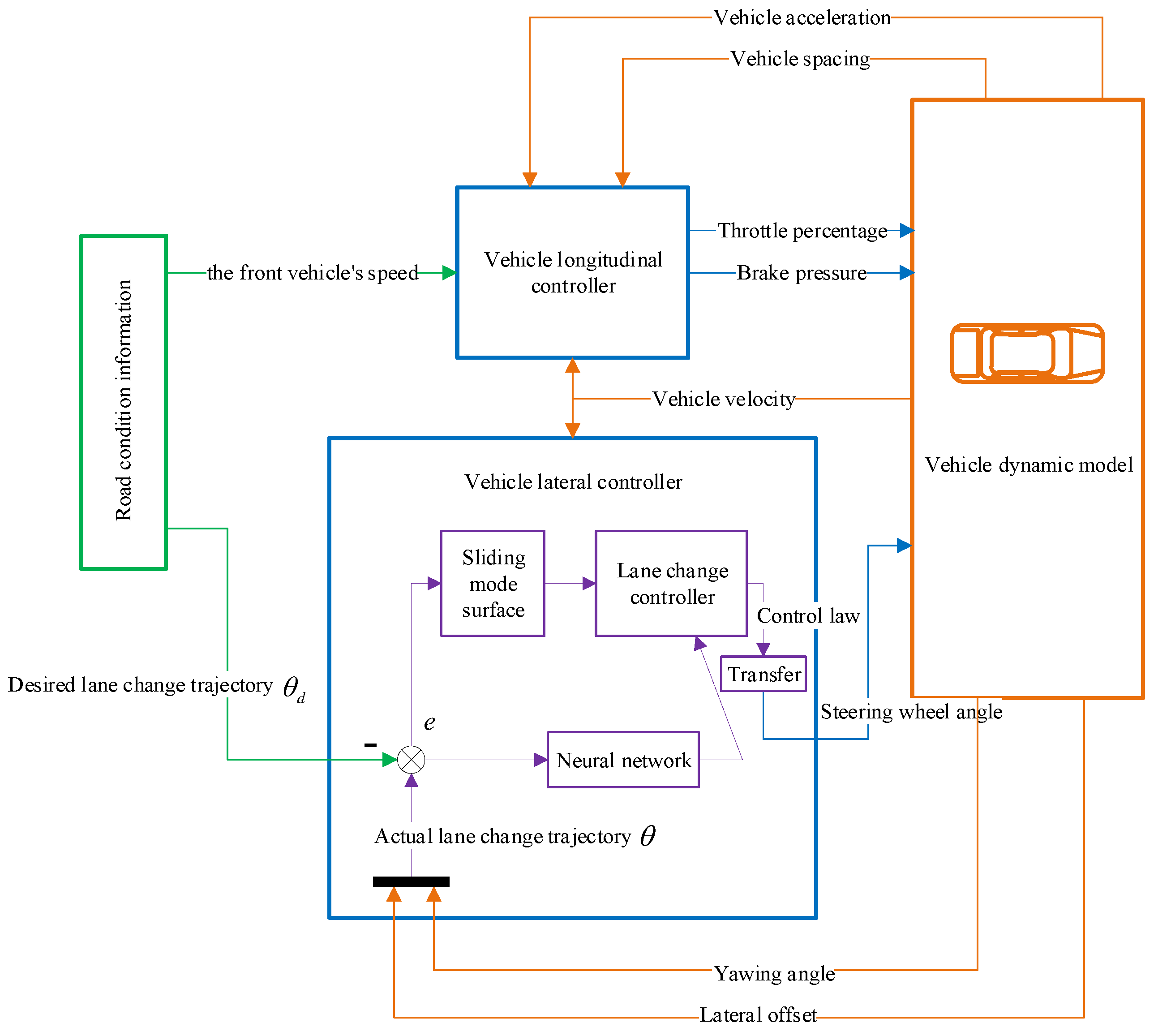
4. Control System and Problem Statement
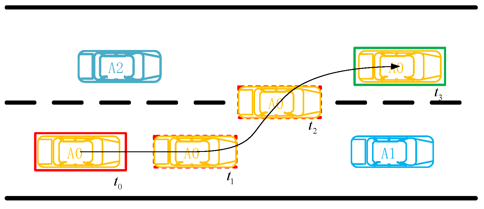
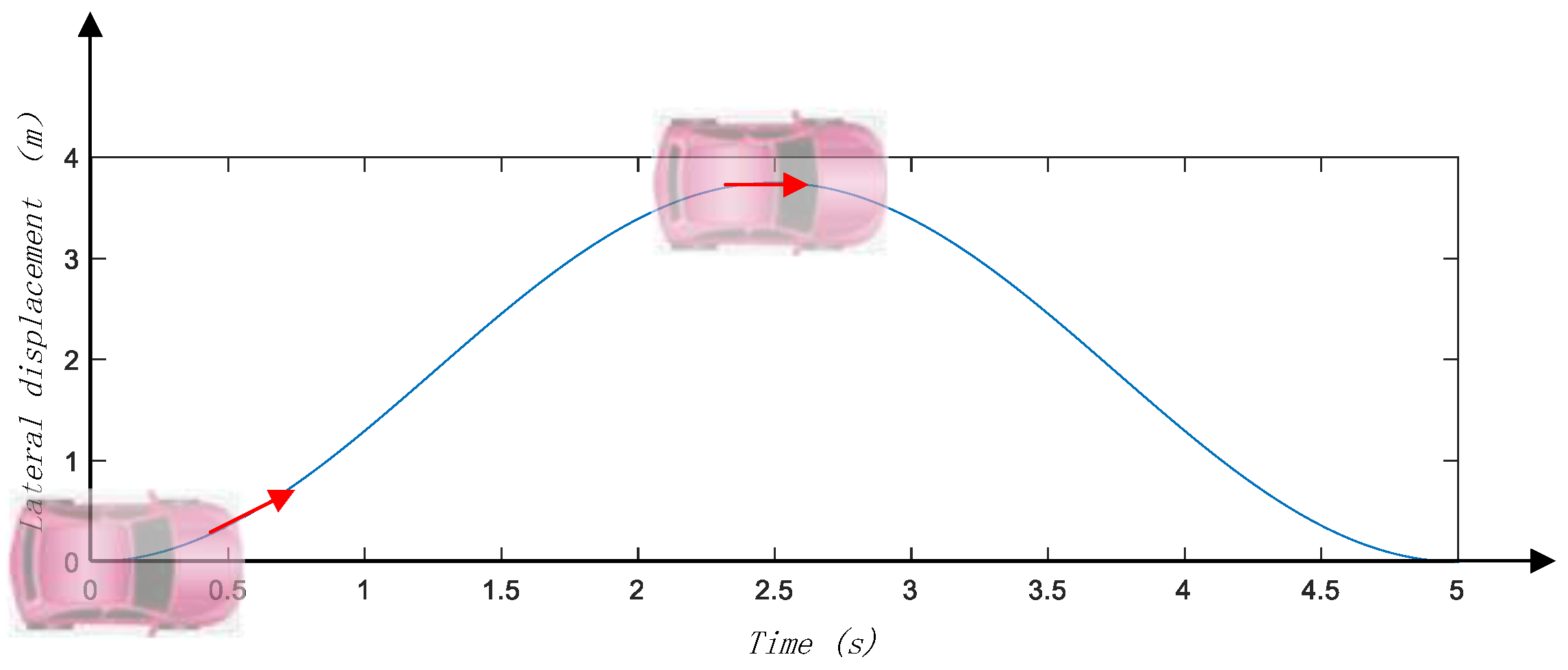
4.1. Path Planning

The cosine function is utilized to build lane-changing trajectory planning in this study:
y ( t ) = 0.5 l w 1 cos π · t l s
According to China’s standard lane width standards, l w is the lane width, which is usually set to l w = 3.75 m. l s represents the vehicle’s longitudinal displacement during lane shift. The cosine lane change trajectory of the vehicle, assuming it completes a lane-changing in five seconds, is illustrated in Figure 3. The cosine function’s lane-changing strategy is simple to calculate, and the lane-changing trajectory is smooth. In addition, the lane-changing trajectory’s lateral acceleration is more gentle, and the vehicle is more comfortable.

4.2. SMC-Based Controller Design

To accomplish the lane change process, the vehicle control system will restrain the vehicle’s movement and force it to follow the intended trajectory strategy. By regulating the steering wheel angle, the lane change process allows the vehicle to follow the intended lane change trajectory.
The ultimate goal of a lane change controller is to manage the steering wheel angle of the vehicle so that it follows the proper lane change trajectory. The vehicle’s tracking error and its derivative are defined as follows:
e = θ θ d
e ˙ = θ ˙ θ ˙ d
e ¨ = θ ¨ θ ¨ d
If the traditional terminal sliding surface s = e ˙ + 1 β e p q , 1 < p q < 2 ,   β > 0 is adopted, the controller design will have a singularity problem when the system converges on the sliding surface. Singularity issues will cause system instability, and the traditional terminal sliding mode function’s convergence rate is slow when the mistake is distant from the phase plane.
The non-singular fast terminal sliding mode surface is proposed in this study to address the slow convergence speed and singularity difficulties of standard terminal sliding mode, as indicated in Equation (8):
s = e + 1 α e γ s i g n ( e ) + 1 β e p q s i g n ( e ˙ )
= e + 1 α s i g γ e + 1 β s i g p q ( e ˙ )
where e γ s i g n ( e ) = s i g γ e , e p q s i g n ( e ˙ ) = s i g p q ( e ˙ ) , α ,   β > 0 , 1 < p q < 2 and γ > p q .
The improved non-singular fast terminal sliding mode control introduces a linear sliding mode and a fast terminal attractor, allowing the system state to swiftly and precisely settle to equilibrium.
Assuming the time from state s 0 to state s = 0 is t r , and the time from state e t r 0 to state e t r + t s = 0 is t s . t s denotes the time to reach equilibrium state. Along the sliding mode (8), the time from any initial condition e 0 to equilibrium state e = 0 is:
t s = 1 β q p · e ( t r ) 0 1 ( u 1 α u γ ) q p d u
The system’s control rate is made up of two components: equivalent control rate u e q and switching control rate u s :
u e q = 1 · θ ¨ d f β q p s i g 2 p q e ˙ γ α s i g γ 1 e · β q p s i g 2 p q e ˙
u s = 1 B d u + sgn s
where > 0 ; therefore, the system’s control rate can be determined as follows:
u = u e q + u s
= 1 · θ ¨ d f β q p s i g 2 p q e ˙ γ α s i g γ 1 e · β q p s i g 2 p q e ˙ + B d u + sgn s
The Lyapunov function is chosen as:
V = 1 2 s 2
Differentiating the Lyapunov function from (13), we have
V ˙ = s s ˙
Theorem 1.
Assume that the upper bound of lumped interference is F. Let Δ f satisfy the hypothesis of Δ f F , and α , β > 0 , 1 < p q < 2 and γ > p q , where p and q are both positive numbers. Then, for nonlinear system model (7), the stability of the closed-loop system can be guaranteed by adopting the sliding mode surface function (8) and the control law (12), and the tracking error can converge to 0 asymptotically in a finite time.
Proof of Theorem 1.
Lyapunov’s theorem is used to prove stability. We can deduce the following from Equation (13):
V ˙ = s e ˙ + γ α s i g γ 1 e e ˙ + 1 β · p q s i g p q 1 e ˙ e ¨
= s e ˙ + γ α s i g γ 1 e e ˙ + 1 β · p q s i g p q 1 e ˙ θ ¨ θ ¨ d
= s e ˙ + γ α s i g γ 1 e e ˙ + 1 β · p q s i g p q 1 e ˙ f + u + Δ f θ ¨ d
= s e ˙ + γ α s i g γ 1 e e ˙ + 1 β · p q s i g p q 1 e ˙ B d u + sgn s
+ Δ f β q p s i g 2 p q e ˙ γ α s i g γ 1 e · β q p s i g 2 p q e ˙
= s e ˙ s i g e ˙ 1 + γ α s i g γ 1 e 1 β · p q s i g p q 1 e ˙ B d u + sgn s + Δ f
= 1 β · p q s i g p q 1 B d u + · s + Δ f · s
1 β · p q s i g p q 1 s B d u + + Δ f 0
The above finishes the proof. □
The system is stable, according to Lyapunov’s second technique. Due to the unknown value of the interference upper bound, a huge interference upper bound must be intentionally imposed, resulting in poor robustness and severe control chattering.

4.3. Enhanced SMC-Based Controller Design

Estimating the upper bound of system lumped disturbance with RBF neural network is a crucial challenge for the enhanced SMC-Based Controller. The upper bound of system lumped interference is estimated using a neural network. Due to the uncertainty of system parameters and external disturbances, robust terms are designed to compensate for the influence caused by disturbances. However, if the robust items are too large, serious chattering will occur in the system. Therefore, this study uses a neural network to estimate the upper bound of system lumped interference. The new proposed self-learning framework is named as NNTSMC, which means a neural network modified version of TSMC (non-singular fast terminal sliding mode control).
Assume that the estimation value of the interference upper bound is set, as the neural network is used to approximate the estimation value of interference upper bound, which can be expressed as: Assuming that the estimation value of the upper bound of interference is set to k ^ , the neural network is used to approximate the estimation value of the upper bound of interference, which may be expressed as:
k ^ = φ ^ T ϕ
where φ is the weight vector of neural network, and n represents the number of nodes of hidden layer. ϕ = ϕ 1 ϕ 2 ϕ n T denotes the output vector of the hidden layer, the Gaussian basis function is used as the membership function, and the output of the i-th node in the hidden layer is:
ϕ i ( x ) = exp ( x H i 2 o 2 i )
where H i is the center vector of the i-th node in the hidden layer, and o 2 i is the base width of the i-th node in the hidden layer, i = 1 , , n .
When the neural network is employed to approach the interference upper bound k ^ , it is assumed that an ideal weight φ * exists, satisfying condition φ * T ϕ Δ f = ε , and ε is the difference between the ideal and real output, satisfying condition k ^ Δ f ε 0 . The weight error of the upper bound of interference estimation by neural network is defined as:
φ ˜ = φ * φ ^ > 0
Based on the above discussion, the improved driving control law can be deduced as follows:
u = u e q + u s = 1 · θ ¨ d f + β q p s i g 2 p q e ˙ + γ α s i g γ 1 e · β q p s i g 2 p q e ˙ 1 k ^ sgn s
Theorem 2.
For the vehicle model under consideration, after the adaptive neural network was added into the original sliding mode control strategy, the designed vehicle lateral control rate was (18), which could still ensure the stability of the controlled system.
The Lyapunov function is designed as:
V = 1 2 s 2 + 1 2 ς φ ˜ T φ ˜
where ς > 0 . Differentiating the Lyapunov function from (19), we have
V ˙ = s s ˙ + 1 ς ˜ ˙ φ T φ ˜
Proof of Theorem 2.
Lyapunov’s theorem is used to prove stability. We can conclude the following from Equation (19).
V ˙ = s e ˙ + γ α s i g γ 1 e e ˙ + 1 β · p q s i g p q 1 e ˙ f + u + Δ f θ ¨ d + 1 ς ˜ ˙ φ T φ ˜ = s e ˙ + γ α s i g γ 1 e e ˙ + 1 β · p q s i g p q 1 e ˙ f + θ ¨ d f + β q p s i g 2 p q e ˙ + γ α s i g γ 1 e · β q p s i g 2 p q e ˙ k ^ sgn s + Δ f θ ¨ d + 1 ς ˜ ˙ φ T φ ˜ = s e ˙ + γ α s i g γ 1 e e ˙ + 1 β · p q s i g p q 1 e ˙ β q p s i g 2 p q e ˙ + γ α s i g γ 1 e · β q p s i g 2 p q e ˙ k ^ sgn s + Δ f + 1 ς ˜ ˙ φ T φ ˜ = s 1 β · p q s i g p q 1 e ˙ k ^ sgn s + Δ f + 1 ς ˜ ˙ φ T φ ˜ = 1 β · p q s i g p q 1 e ˙ φ ^ T ϕ sgn s + Δ f s + 1 ς ˜ ˙ φ T φ ˜ = 1 β · p q s i g p q 1 e ˙ φ ^ T ϕ s Δ f · s + 1 ς ˜ ˙ φ T φ ˜
The weight adaptive law of the neural network is built as follows since the optimal weight φ * is a constant value:
˜ ˙ φ = ^ ˙ φ = ς ϕ s
Substitute Equation (22) into Equation (20) to obtain:
V ˙ = 1 β · p q s i g p q 1 e ˙ φ ^ T ϕ s Δ f · s 1 ς ς ϕ s φ * φ ^
= 1 β · p q s i g p q 1 e ˙ φ ^ T ϕ s Δ f · s s ϕ φ * φ ^
1 β · p q s i g p q 1 e ˙ s φ * T ϕ Δ f
= 1 β · p q s i g p q 1 e ˙ s ε 0
The above finishes the proof. □
The Lyapunov function is negative semidefinite, according to the second method of Lyapunov, and the control rate proposed in this study can ensure system stability. It can be seen from the above proof process that the disturbance upper bound is estimated, and the disturbance compensation is carried out by using an adaptive neural network, which ensures the stability of the system and solves the chattering phenomenon caused by excessive robust gain.
Through the above analysis, it can be seen that, based on the vehicle dynamics model and road condition information, the lane changing control strategy oriented to the desired lane-changing trajectory can be designed. The framework overview of vehicle lateral and longitudinal integrated controller is shown in Figure 4. The lane change control method integrates the sliding mode control method and neural network, which has certain anti-disturbance ability. Lane-changing control is the core of the lateral controller. The lateral controller and longitudinal controller work together to complete the lane change driving process.

5. Experiments and Discussion

In order to verify the performance of the lane-changing controller based on the proposed control strategy, several experiments were designed. The above-mentioned lane-changing trajectory planning and control methods are simulated and evaluated, and the simulation data are reviewed to confirm the correctness and efficacy of the chosen control approach.
MATLAB and CarSim software are chosen for co-simulation. First of all, the vehicle model is constructed in the CarSim software. Then, combined with the control module in MATLAB/Simulink-CarSim co-simulation environments, we can execute the test of the control strategy introduced above. Finally, the driving process of the vehicle is simulated, and the test result can be observed.

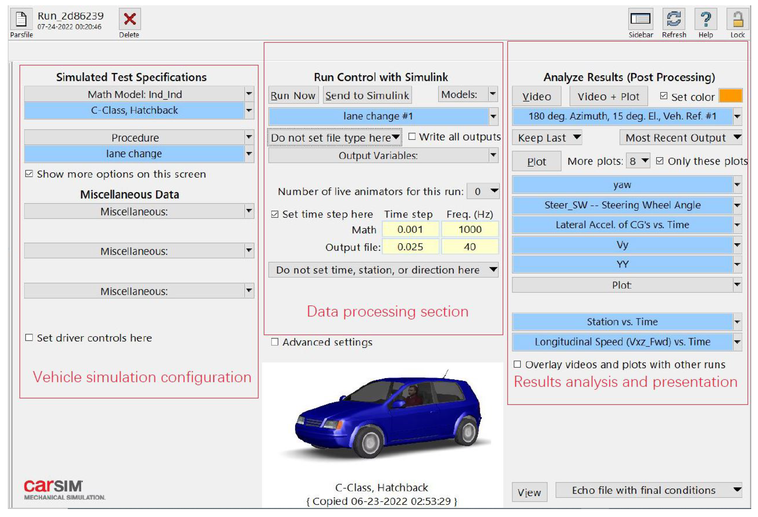
5.1. Experimental Parameter Configuration
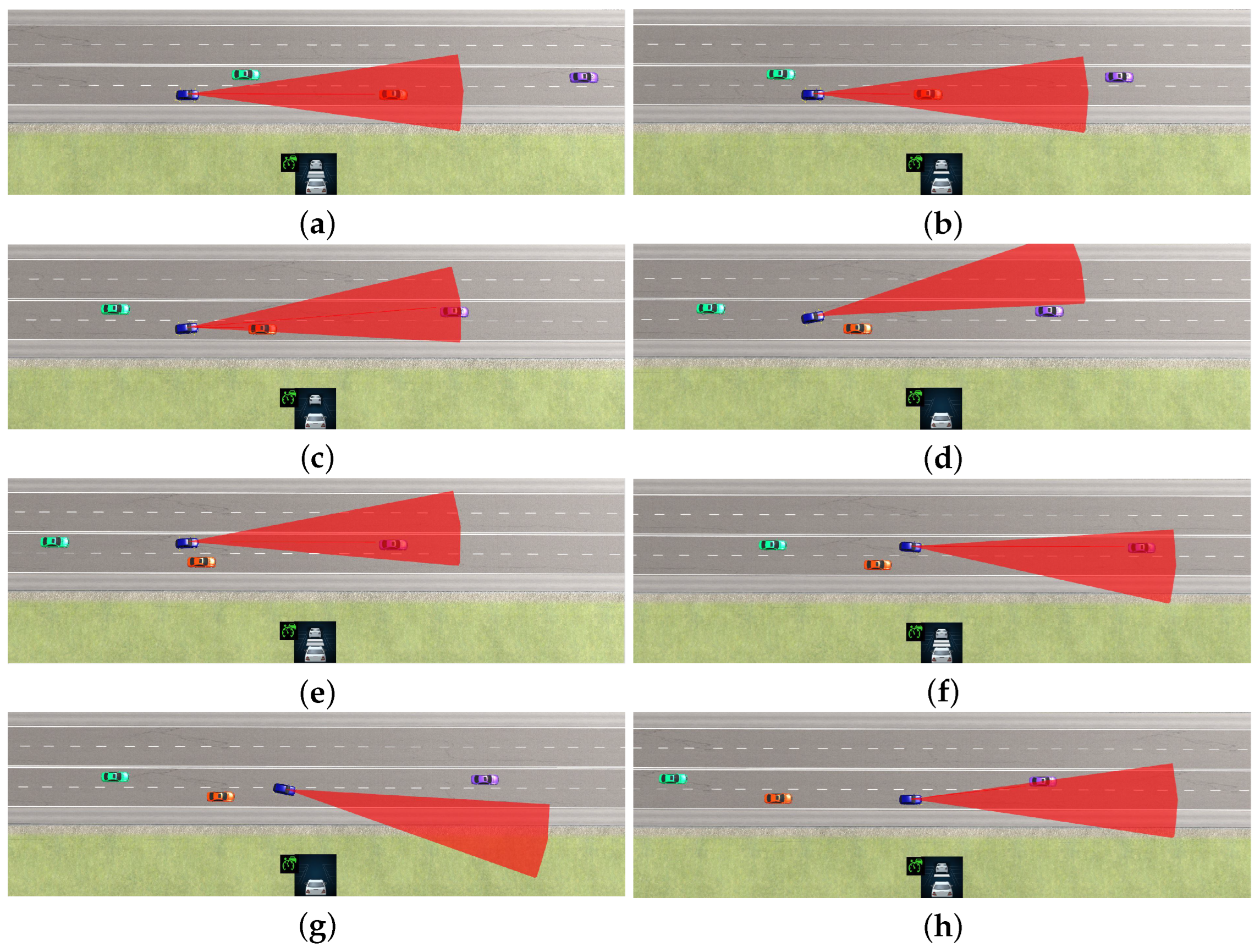
In this paper, the C-class vehicle was selected for the simulation experiment, and the experimental parameter of the whole vehicle was established in CarSim software. Figure 5 demonstrates the main interface of the CarSim simulation software.
The CPU is Intel(R) [email protected] Ghz, and the RAM is 64 GB, in addition to the hardware and software environment setup employed in the simulation experiment. The main parameters of the vehicle are shown in Table 1.
Other parameters, such as the power system coefficient, brake system coefficient, and body air resistance coefficient, all adopt the default specifications of the vehicle in the software. Road parameter settings are modified based on the Road model in “Road: 3D Surface” in CarSim software 2019.0. This software is provided by Mechanical Simulation Corporation, Mountain View, CA, USA.The road model is a two-way four-lane freeway, and the double solid lines in the middle are road dividers in different directions. The track of the experimental road is straight. The length and the width of the lane are 1000 m and 3.75 m, respectively. The road friction coefficient is 0.65, while the other parameters of the road model remain unchanged.

5.2. Scenario Study

This study verifies the performance of the proposed lane-changing strategy in the MATLAB/Simulink-CarSim co-simulation environments. CarSim provides vehicle dynamics model and vehicle-related parameter information. The algorithm of the lane change controller is built in Simulink. In the co-simulation, the steering wheel angle is input into the vehicle dynamics model, and the relative position information, lateral and longitudinal velocity, yaw angle and other related parameters of the vehicle are output variables, and these state variables are input into the lane change controller. The steering wheel angle can be output to the vehicle dynamics model for vehicle attitude control, and the lane change controller can obtain the new control law value based on the input vehicle-related parameter information. The mission of trajectory tracking control is ultimately accomplished by the vehicle dynamics model, which circulates the process and outputs the vehicle state information at the subsequent instant.
In order to verify the effectiveness of the lane-changing control strategy proposed in this paper, two typical lane-changing test scenarios are constructed in the following experiment.
Scenario A tested the scenario in which the ego vehicle changed lanes from the current lane and continued driving in another lane. This scenario primarily validates the proposed framework for dealing with emergency obstacles in front of the current lane or being forced to change lanes because the front vehicle is driving at a low speed. In this scenario, the lane change operation only needs to be performed once.
Experimental scenario B, namely overtaking, tested the scenario in which a vehicle changed lanes from the current lane and then changed lanes again into the original lane to continue driving. This scenario primarily validates the performance of the proposed framework in a similar environment where overtaking is required. The process of overtaking is a combination of two lane-change processes. Finally, the vehicle completed the lane change process while remaining in the original lane.
Figure 6 is an animated screenshot of scenario B. As can be seen from the animation screenshot, before lane change, the ego vehicle runs in the original lane with a good distance. Due to the slow speed of the vehicle in front in the original lane, the distance between vehicles gradually decreases. After the lane-changing demand is generated and the lane-changing decision is formed and executed after the lane-changing condition judgment, the target vehicle gradually moves from the original lane to the target lane along the planned lane-changing trajectory with a small driving error. At the end of the lane change, the target vehicle runs smoothly in the target lane. The screenshot consists of eight sub-images. Figure 6a shows the vehicle perceiving the vehicle ahead in the current lane. Figure 6b shows that the test vehicle has moved close to the front vehicle along the current lane because the speed of the front car is low, and it needs to be forced to change lanes. Figure 6c,d represent the first lane change process, and Figure 6e represents the completion of the first lane change. Figure 6f,g show the second lane-change process. Figure 6h shows the completion of the second lane change. Traffic continued in the same lane.

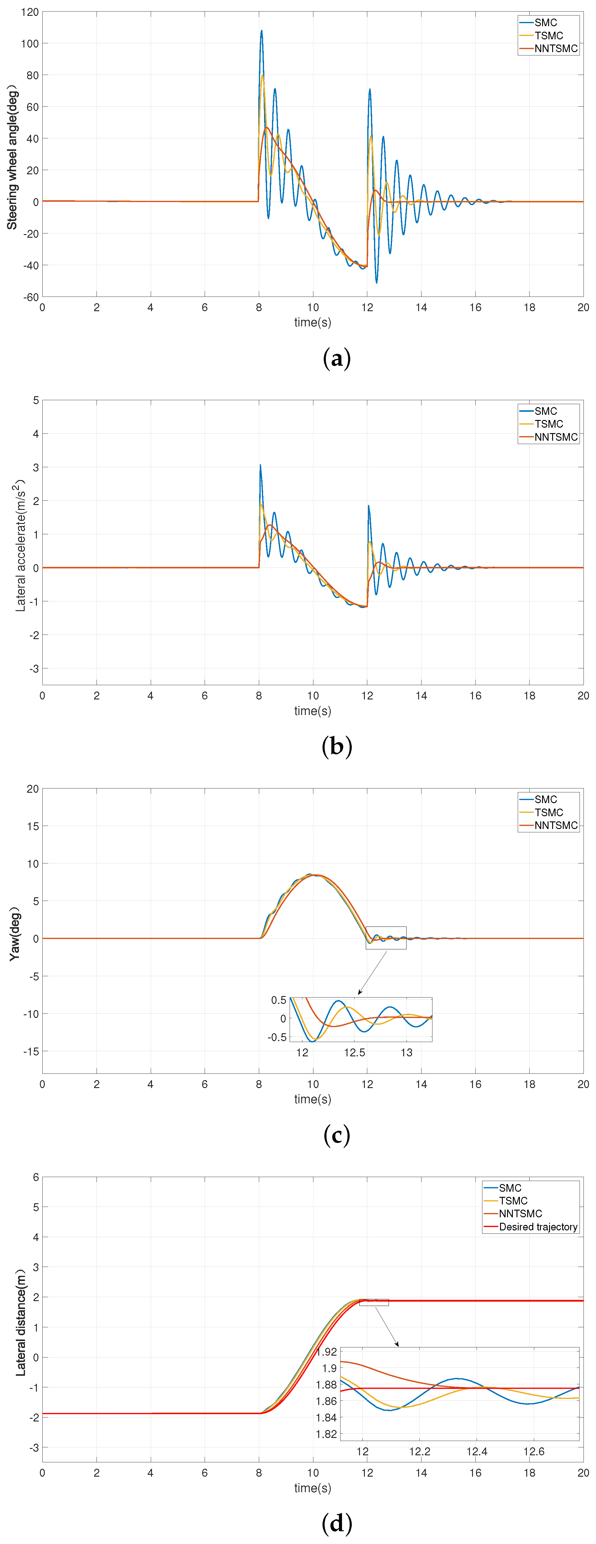
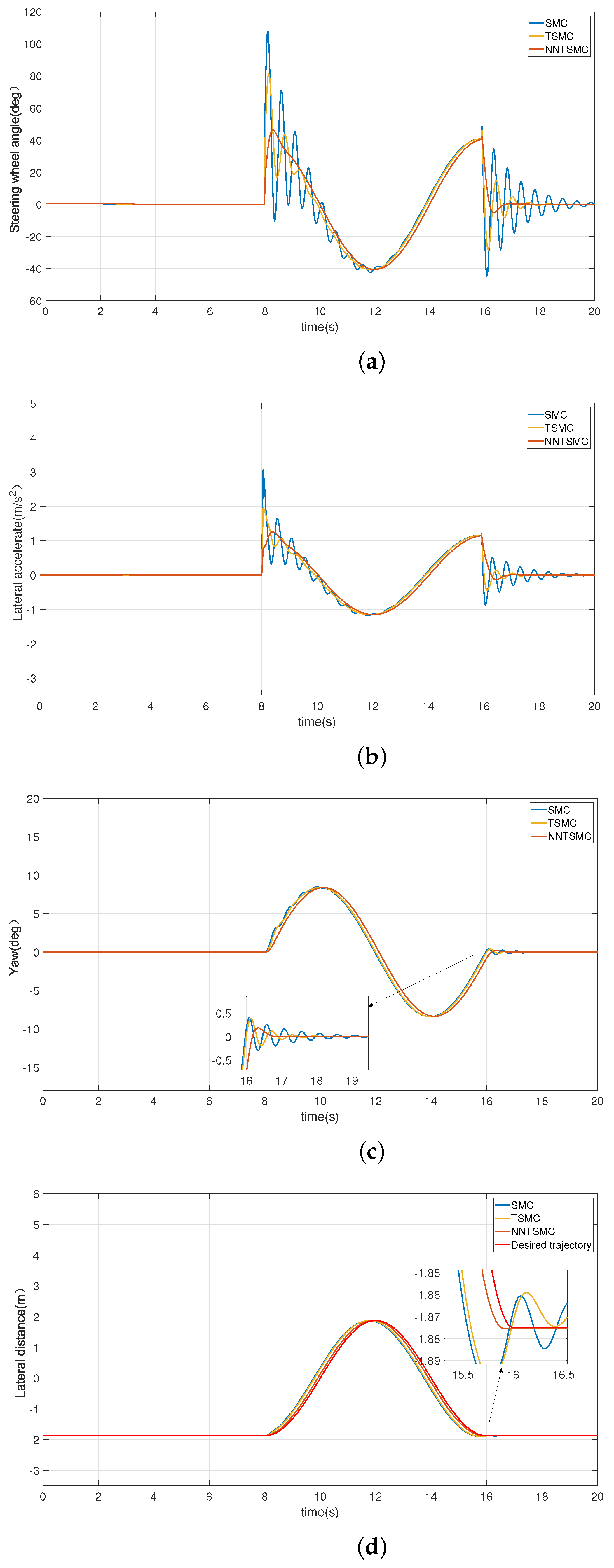
5.3. Verification and Results Discussion

Classical SMC, TSMC, and the method proposed in this study were used for comparison. Two scenario tests were conducted using a MATLAB/Simulink-CarSim co-simulation experimental platform for self-driving vehicles. These tests were carried out on two-way four lane roads with a width of 3.75 m, and the ego vehicle speed is 10 m/s.
This paper takes the low-speed lane-changing scenario as an example, and the results of the two lane change scenarios are shown in Figure 7 and Figure 8, respectively. In this paper, the results of different control methods are plotted in the same picture. Figure 7 shows four diagrams with important state information about the vehicle. As can be seen from the figure, the start time of the lane changing process is the time point of 8 s, and the lane-changing duration is 4 s. As can be seen from Figure 7a, among the three methods, the lane change effect of the controller designed by the SMC method is the most unstable. The SMC has a maximum wheel angle of more than 100 degrees, which is a very drastic lane change operation and even dangerous on the actual road. TSMC performed much better than SMC. Using TSMC method, it can be seen that the maximum peak angle of the commutator wheel is more than 40 degrees. The best performance is NNTSMC, which not only has the best performance in the peak angle of the steering wheel, but also has a stable performance in the whole lane change process. In the whole lane change process, the NNTSMC’s curve is the smoothest from the result. In comparison, SMC and TSMC methods are much less stable.
Lateral acceleration is an important parameter in the process of lane change. As can be seen from Figure 7b, the maximum peak value of SMC’s lateral acceleration reaches 3.065 m/s2, indicating a large overshoot of vehicle state at the instant of lane change. In addition, in the process of switching, the curve of SMC method switches frequently, which is very unstable. The performance of TSMC has been improved, but the maximum peak value is still 1.925 m/s2, and there is occasional instability in the process of lane change. The change of the acceleration of NNTSMC is the smoothest, and the peak value is 1.269 m/s2. From the perspective of lane changing process, the proposed method has the most stable manifestation. Therefore, NNTSMC still has the best performance among the three methods in terms of lateral acceleration.
A similar conclusion can be drawn from Figure 7c. NNTSMC has the best performance in the angle index of yaw, and the local magnification effect of the original image can be seen from the enlarged small block diagram. We can find that the controller designed by the proposed method has the quickest transition process, the fastest control, and the highest precision. Yaw can get back to zero at the end of the lane change very accurately.
In this paper, lateral distance is also a very important measurement index. The accuracy of lateral displacement reflects the accuracy of the vehicle controller. The smaller the error between the measured distance value and the desired value, the better the control effect of the method. From Figure 7d, we can see the lateral distance results of multiple methods. Although all methods finally stabilized at the value of about 1.875 m after lane change, only NNTSMC showed the best performance in the transition process as shown in the enlarged figure. High control precision and rapid control process are the abilities that an excellent control algorithm needs at the same time.
Scenario B is an upgraded version of Scenario A. The common point of the two experiments is that the start time of the lane changing process is 8 s. The difference is that the lane change in scenario B lasts eight seconds. Therefore, the first four seconds of Figure 8a–d is the same process as Figure 7. The difference is, in the second lane change process, the four seconds it takes to switch back into the original lane in Scenario B. From these four subgraphs in Figure 8, it can be seen that the overall performance of NNTSMC maintains outstanding results in the continuous lane change scenario. In terms of wheel angle stability, safety, and comfort reflected by lateral acceleration, and further lateral distance accuracy, the proposed method has the best performance. In comparison, both SMC and TSMC failed to show better accuracy and stability.
Specific experimental results of the MATLAB/Simulink-CarSim co-simulation, including the maximum lateral acceleration and maximum lateral error, are summarized in Table 2. We can make a comparative analysis of the three methods participating in the comparative experiment from the vertical and horizontal dimensions in Table 2. The two variables listed are very relevant to the process of lane change. The maximum lateral acceleration and maximum lateral error can reflect the driving comfort and the accuracy of trajectory tracking during the process of lane-changing, respectively. All test data of the proposed method are shown in bold in Table 2. As can be seen from Table 2, when the vehicle with the lane-changing controller proposed in this paper tracks the corresponding trajectory under different scenarios, the lateral acceleration changes stably without sharp points, and meets the requirements of the vehicle when performing lane-changing actions.
Taking the maximum lateral acceleration as an example, the maximum values of the proposed method in the two scenarios are 1.269 and 1.272, respectively. Compared with SMC and TSMC, the new method achieves significant improvement of 58.6% and 34.1% in scenario A, respectively. Furthermore, in scenario B, the new method achieves a significant improvement of 58.5% and 35.3% over SMC and TSMC, respectively. A similar effect can be seen from the maximum lateral error. In scenario A and scenario B, the new method achieves results of 0.118 and 0.137, respectively, which is significantly better than the other two representative methods. Compared with SMC and TSMC, the new method achieves significant improvement of 58.0% and 53.2% in scenario A, respectively. In scenario B, the new method achieves a significant improvement of 63.7% and 58.6%.
Regardless of the scenario, the vehicle using the proposed method can adjust its state in a short amount of time, and the lateral error is always kept within the smallest range, demonstrating that the vehicle has good handling stability for the lane change trajectory described in the paper. In conclusion, compared with SMC, the proposed method has a performance improvement of at least 58.0% and a performance improvement of at least 34.1% compared with TSMC.
In conclusion, the results of the above two experimental scenarios show that the lane changing controller designed by the method proposed in this paper achieves ideal effects and is competent for complex lane changing scenarios. The results show that the designed lane change control method meets the requirements of lane change maneuver and has pretty good handling and stability, which verifies the effectiveness of the lane change control strategy. Ensure that the vehicle can meet the passenger’s requirements for speed and comfort in the actual lane change.

6. Conclusions

This paper proposes a novel lane-changing control strategy based on the NNTSMC method aiming at improving lane-changing reliability and driving comfort. Lane-changing control strategy integrates a non-singular fast terminal sliding mode control method and neural networks, which possess certain anti-disturbance ability.
As the key technology of vehicle intelligent driving, lane-changing control has great research significance. Based on the established vehicle dynamics model and lane-changing controller, the results are verified in MATLAB/Simulink-CarSim co-simulation environments. CarSim provides a vehicle dynamics model and vehicle related parameter information. The lane-changing controller is constructed in Simulink.
In order to verify the function of the lane-changing controller based on the proposed control strategy, several experiments are also designed in this paper. Simulation experiments with two scenario tests performed on the co-simulation platform confirmed the effectiveness and superiority of the proposed control scheme over the traditional SMC approach and TSMC. The lane-changing trajectory planning model and lane-changing control model established above are simulated and tested. Through the analysis of simulation data, the superiority and effectiveness of the control strategy are verified. The proposed method, in comparison to SMC, has a performance improvement of at least 58.0%, and compared to TSMC, it has a performance improvement of at least 34.1%. Simulation results show that the proposed method can make the vehicle track the lane center with a small error and maintain good driving quality.
Although the test results are ideal, compared with the actual lane-changing scene, there are inevitably some problems that have not been considered comprehensively. In the future, we will attempt to conduct the verification experiment using a physical vehicle. In practical applications, when modeling the vehicle dynamics, the uncertainty of its parameters and the uncertainty of the external environment, such as the friction of mechanical components, wheel skids, etc., will affect the accuracy of trajectory tracking. Therefore, when designing a higher standard lane change controller, it is essential to establish a dynamic model with richer information and base the control algorithm on it.

Author Contributions

Conceptualization, C.W.; modeling, simulation, and validation, C.W.; writing, original draft preparation, C.W.; supervision and critical review, Y.D. All authors have read and agreed to the published version of the manuscript.

Funding

This research was funded by the Shanghai Municipal Education Commission, the Major Natural Science Project of Scientific Research and Innovation Program (No. 2021-01-07-00-07-E00092), the Ministry of Science and Technology of the People’s Republic of China, and the National Key Research and Development Program Grant/No. 2021YFB1600100.

Institutional Review Board Statement

Not applicable.

Informed Consent Statement

Not applicable.

Data Availability Statement

Not applicable.

Conflicts of Interest

The authors declare no conflict of interest.

References

  1. Zheng, Z. Recent developments and research needs in modeling lane changing. Transp. Res. Part B Methodol. 2014, 60, 16–32. [Google Scholar]
  2. Ishtiak, A.; Alan, F.K.; Nagui, M.R.; Thomas, C.; Shams, T. Characterizing lane changing behavior and identifying extreme lane changing traits. Transp. Lett. 2022. [Google Scholar] [CrossRef]
  3. Mahmood, A.A.; Selvakumar, M.; Badiea, A.M.; Zeyad, G.A.; Amjad, Q.; Abdullah, J.A.; Gharbi, A.; Amer, A.S.; Khalil, A. Provably Secure with Efficient Data Sharing Scheme for Fifth-Generation (5G)-Enabled Vehicular Networks without Road-Side Unit (RSU). Sustainability 2022, 14, 9961. [Google Scholar] [CrossRef]
  4. Cui, Y.; Wu, J.Q.; Xu, H.; Wang, A.B. Lane change identification and prediction with roadside LiDAR data. Opt. Laser Technol. 2020, 123, 105934. [Google Scholar] [CrossRef]
  5. Panichpapiboon, S.; Leakkaw, P. Lane change detection with smartphones: A steering wheel-based approach. IEEE Access 2020, 8, 91076–91088. [Google Scholar] [CrossRef]
  6. Woo, H.; Sugimoto, M.; Madokoro, H.; Sato, K.; Tamura, Y.; Yamashita, A.; Asama, H. Goal estimation of mandatory lane changes based on interaction between drivers. Appl. Sci. 2020, 9, 3289. [Google Scholar] [CrossRef]
  7. Mahmood, A.A.; Mohammed, A.; Iznan, H.H.; Selvakumar, M.Z. Survey of Authentication and Privacy Schemes in Vehicular Ad Hoc Networks. IEEE Sens. J. 2021, 21, 2422–2433. [Google Scholar]
  8. Mahmood, A.A.; Mohammed, A.; Selvakumar, M.; Iznan, H.H. A Secure Pseudonym-Based Conditional Privacy-Preservation Authentication Scheme in Vehicular Ad Hoc Networks. Sensors 2022, 22, 1696. [Google Scholar] [CrossRef]
  9. Mahmood, A.A.; Mohammed, A.; Selvakumar, M.; Iznan, H.H. Password-Guessing Attack-Aware Authentication Scheme Based on Chinese Remainder Theorem for 5G-Enabled Vehicular Networks. Appl. Sci. 2022, 12, 1383. [Google Scholar] [CrossRef]
  10. Hu, C.; Wang, Z.; Qin, Y.; Huang, Y.; Wang, J.; Wang, R. Lane Keeping Control of Autonomous Vehicles With Prescribed performance considering the rollover prevention and input saturation. IEEE Trans. Intell. Transp. Syst. 2020, 21, 3091–3103. [Google Scholar]
  11. Gipps, P.G. A model for the structure of lane-changing decision. Transp. Res. Part B Methodol. 1986, 20, 403–414. [Google Scholar] [CrossRef]
  12. Yang, Q.I.; Koutsopoulos, H.N. A model for the structure of lane-changing decision. Transp. Res. C 1996, 4, 113–129. [Google Scholar] [CrossRef]
  13. Barcelo, J.; Ferrer, J.L.; Grau, R. A Route Based Variant of the AIMSUM2 Microsimulation Model. In Proceedings of the Steps Forward Intelligent Transport Systems World Congress, Yokohama, Japan, 9–11 November 1995. [Google Scholar]
  14. Nagel, K.; Wolf, D.E.; Wagner, P. Two-lane traffic rules for cellular automata: A systematic approach. Phys. Rev. E Stat. Phys. Plasmas Fluids Relat. Interdiscip. Top. 1997, 58, 1425–1437. [Google Scholar] [CrossRef]
  15. Benekohal, R.F. Traffic Congestion and Traffic Safety in the 21st Century: Challenges, Innovations, and Opportunities, Chicago, Illinois, June 8–11, 1997: Proceedings of the Conference Sponsored by Urban Transportation Division, ASCE, Highway Division, ASCE; American Society of Civil Engineers: New York, NY, USA, 1997. [Google Scholar]
  16. Hidas, P. Modeling lane changing and merging in microscopic traffic simulation. Transp. Res. C 2002, 10, 351–371. [Google Scholar] [CrossRef]
  17. Chen, L.; Qin, D.F.; Xu, X.; Cai, Y.F.; Xie, J. A path and velocity planning method for lane changing collision avoidance of intelligent vehicle based on cubic 3-D Bezier curve. Adv. Eng. Softw. 2019, 132, 65–73. [Google Scholar] [CrossRef]
  18. Zhang, R.; Zhang, Z.; Guan, Z.; Li, Y.; Li, Z. Autonomous lane changing control for intelligent vehicles. Clust. Comput. 2018, 22, 8657–8667. [Google Scholar] [CrossRef]
  19. Ding, Y.; Zhuang, W.C.; Wang, L.M.; Liu, J.X.; Guvenc, L.; Li, Z. Safe and optimal lane-change path planning for automated driving. Proc. Inst. Mech. Eng. Part D J. Automob. Eng. 2020, 235, 1070–1083. [Google Scholar] [CrossRef]
  20. Feng, Z.Q.; Song, W.J.; Fu, M.Y.; Yang, Y.; Wang, M.L. Decision-making and path planning for highway autonomous driving based on spatio-temporal lane-change gaps. IEEE Syst. J. 2021, 16, 3249–3259. [Google Scholar] [CrossRef]
  21. You, F.; Zhang, R.; Lie, G.; Wang, H.; Wen, H.; Xu, J. Trajectory planning and tracking control for autonomous lane change maneuver based on the cooperative vehicle infrastructure system. Expert Syst. Appl. 2015, 42, 5932–5946. [Google Scholar] [CrossRef]
  22. Ren, D.; Zhang, J.; Zhang, J.; Cui, S. Trajectory planning and yaw rate tracking control for lane changing of intelligent vehicle on curved road. Sci. China Technol. Sci. 2011, 54, 630–642. [Google Scholar] [CrossRef]
  23. Wang, L.; Zhao, X.; Su, H.; Tang, G. Lane changing trajectory planning and tracking control for intelligent vehicle on curved road. SpringerPlus 2016, 5, 1150. [Google Scholar]
  24. Jing, C.; Shu, H.; Shu, R.; Song, Y. Integrated control of electric vehicles based on active front steering and model predictive control. Sci. China Technol. Sci. 2022, 121, 105066. [Google Scholar] [CrossRef]
  25. Zhang, B.; Zhang, J.W.; Liu, Y.; Guo, K.H.; Ding, H.T. Planning flexible and smooth paths for lane-changing manoeuvres of autonomous vehicles. IET Intell. Transp. Syst. 2021, 15, 200–212. [Google Scholar]
  26. Ren, D.; Zhang, J.; Cui, S.; Zhang, J. Variable structure control for platoon lane change in automated highway systems. J. Harbin Inst. Technol. 2009, 41, 109–114. [Google Scholar]
  27. Qi, Z.; Yang, Z.; Huang, Y. Lane Change Track Control for Intelligent 4WS Vehicle Based on Fuzzy Adaptive PID. Chin. J. Automot. Eng. 2012, 2, 379–384. [Google Scholar]
  28. Guo, L.; Ge, P.; Yue, M.; Zhao, Y. Lane Changing Trajectory Planning and Tracking Controller Design for Intelligent Vehicle Running on Curved Road. Math. Probl. Eng. 2014, 2014, 478573. [Google Scholar] [CrossRef] [Green Version]
  29. Chen, C.; Shu, M.; Wang, Y.; Liu, R. Robust H Control for Path Tracking of Network-Based Autonomous Vehicles. Math. Probl. Eng. 2020, 2020, 2537086. [Google Scholar] [CrossRef]
  30. Li, H.; Huang, J.; Yang, Z.; Hu, Z.; Yang, D.; Zhong, Z. Adaptive robust path tracking control for autonomous vehicles with measurement noise. Int. J. Robust Nonlinear Control 2022, 32, 7319–7335. [Google Scholar]
  31. Luo, F.; Zeng, X. Research on path following algorithm for autonomous vehicle based on multiple look-ahead points. Mechatronics 2018, 6, 17–22. [Google Scholar]
  32. Chen, X.; Zhou, B.; Wu, X. Autonomous vehicle path tracking control considering the stability under lane change. Proc. Inst. Mech. Eng. Part I J. Syst. Control Eng. 2021, 235, 1388–1402. [Google Scholar]
Figure 1. Schematic diagram of the vehicle lane-changing scenario.
Applsci 12 11000 g001
Figure 2. Schematic diagram of the Vehicle Kinematic Model.
Applsci 12 11000 g002
Figure 3. Diagram of a cosine lane change trajectory.
Applsci 12 11000 g003
Figure 4. The framework overview of vehicle lateral and longitudinal integrated controllers.
Applsci 12 11000 g004
Figure 5. Main interface of the CarSim simulation software.
Applsci 12 11000 g005
Figure 6. Simulation animation screenshot of Scenario B.
Applsci 12 11000 g006
Figure 7. The experimental results of Scenario A.
Applsci 12 11000 g007
Figure 8. The experimental results of Scenario B.
Applsci 12 11000 g008
Table 1. Main parameters configuration of the vehicle model.
ParameterNumerical Value
Vehicle sprung mass1723 kg
Internal engine power125 N·m
Peak engine torque267.3 kW
Vehicle length2578 mm
Vehicle width1739 mm
Vehicle heigth1478 mm
Distance between mass center and front axle1232 mm
Roll inertia1243.1 kg·m2
Pitch inertia4331.6 kg·m2
Yaw inertia4175 kg·m2
Frontal area1.6 m2
Road friction coefficient0.65
Table 2. Experimental results of the co-simulation.
Method Name V x = 10 (m/s)
Scenario AMaximum lateral acceleration (m/s2)SMC3.065
TSMC1.925
Proposed1.269
Maximum lateral error (m)SMC0.281
TSMC0.252
Proposed0.118
Scenario BMaximum lateral acceleration (m/s2)SMC3.065
TSMC1.965
Proposed1.272
Maximum lateral error (m)SMC0.377
TSMC0.331
Proposed0.137
Publisher’s Note: MDPI stays neutral with regard to jurisdictional claims in published maps and institutional affiliations.

