Article

Real-Time Risk Assessment for Road Transportation of Hazardous Materials Based on GRU-DNN with Multimodal Feature Embedding

1
National Engineering and Research Center for Mountainous Highways, China Merchants Chongqing Communications Research & Design Institute Co., Ltd., Chongqing 400067, China
2
Logistics Research Center, Shanghai Maritime University, Shanghai 201306, China
3
Key Laboratory of Road and Traffic Engineering of the Ministry of Education, Tongji University, Shanghai 201804, China
4
School of Electronic and Control Engineering, Chang’an University, Xi’an 710064, China
*
Author to whom correspondence should be addressed.
These authors contributed equally to this work.
Appl. Sci. 2022, 12(21), 11130; https://doi.org/10.3390/app122111130
Submission received: 27 September 2022 / Revised: 27 October 2022 / Accepted: 30 October 2022 / Published: 2 November 2022

Abstract

:
In this paper, a gated recurrent unit–deep neural network (GRU-DNN) model integrated with multimodal feature embedding (MFE) is developed to evaluate the real-time risk of hazmat road transportation based on various types of data for contributing factors. MFE was incorporated into the framework of a deep learning model in which discrete variables, continuous variables, and images were uniformly embedded. GRU is a pre-trained sub-model, and the DNN is able to directly use the relative structure and weights of the GRU, improving the poor classification and recognition results due to insufficient samples. Additionally, the model is trained and validated based on hazmat road transportation database consisting of 2100 samples with 20 real-time contributing factors and four risk levels in China. The accuracy (ACC), precision (PR), recall (RE), F1-score (F1), and areas under receiver-operating-characteristic curves (AUC) of the proposed model and other commonly used models are compared as performance measurements in numerical examples. Finally, Carlini & Wagner attack and three defenses of adversarial training, dimensionality reduction and prediction similarity are proposed in the training to improve the robustness of the model, alleviating the impact of noise and error on small-sized samples. The results demonstrate that the average ACC of the model reaches 93.51% and 87.6% on the training and validation sets, respectively. The prediction of accidents resulting in injury is the most accurate, followed by fatal accidents. Combined with the RE of 89.0%, the model exhibits excellent performance. In addition, the proposed model outperforms other widely used models based on the overall comparisons of ACC, AUC, F1 and PR-RE curve. Finally, prediction similarity can be used as an effective approach for robustness improvement, with the launched adversarial attacks being detected at a high success rate.

1. Introduction

According to statistics, the transportation of hazardous materials (hazmat) is still on the rise in China. Over 1730 million tons of hazmat were transported across China in 2020 [1]. Approximately 95% of hazardous materials are shipped via long-distance transportation, and nearly 69% are transported by road [2]. During the course of road transportation, there were approximately 1416 hazmat accidents in China between 2010 and 2015 [3]. Road transportation administrations (RTAs) [4] are concentrating their attention on real-time risk assessment for the road transportation of hazmat, since hazmat can be combustible, explosive, toxic, corrosive, or radioactive [5,6], despite the fact that the accident rate for such transportation is quite low (generally from 10−8 to 10−6/km) [7,8]. Road tankers with hazmat can be represented as potential “mobile bombs” that could result in serious casualties, property damage, and environmental pollution [9,10,11,12,13]. Real-time risk assessment of hazmat transportation is challenging due to the numerous risk factors, the unknown operational status of road tanks, and the variable nature of transportation environments [14]. Fortunately, GPS tracking and dashboard cameras have been compulsory in road tankers transporting hazmat in China in recent years. Real-time risk assessment for road transportation of hazmat becomes feasible when the operational condition of road tankers is monitored and various data are simultaneously transferred to RTAs.
Risk assessment is one of the top priorities in the investigation of hazmat transportation, serving as the basis for risk mitigation [6,15,16,17]. In traffic safety studies, the risk is represented by the occurrence of accidents, which is a binary variable (i.e., accident vs. non-accident) [18]. However, the accident rate for hazmat transportation is relatively low, with severity being the most striking feature for hazmat transportation accidents. Hence, the risk of road transportation of hazmat is evaluated on the basis of the occurrence and severity of accidents [19,20]. The relationship between road transportation risk and contributing factors can be assessed on the basis of either parametric or nonparametric approaches. Parametric approaches include traditional statistical models [21,22,23,24,25,26,27], while nonparametric approaches are based on machine learning techniques [1,3,28].
Typical assumptions in traditional statistical models include deterministic data distribution and the existence of a linear relationship between the independent and dependent variables. In contrast, machine learning techniques are able to overcome these limitations and achieve better performance [29]. One of the popular machine learning methods in real-time risk assessment of hazmat road transportation is the Bayesian network-based model [1,3]. This method consists of an easy-to-update model and provides a more reliable and practical forecast [30]. However, contributing factors in the Bayesian network-based model are always discrete, meaning that it cannot accommodate various types of data from GPS tracking and dashboard cameras in road tankers carrying hazmat.
In the literature, mechanical and structural problems with road tanks, road conditions, weather conditions, types of hazmat, and driver error are the main contributing factors reported to expose hazmat transportation to risk of accident occurrence [31,32,33,34,35]. These factors include discrete variables (e.g., weather), continuous variables (e.g., travel speed) and real-time images (e.g., fatigue driving behavior). Compared with other learning architectures, deep learning can model complex non-linear relationships using distributed and hierarchical feature representation [36,37,38]. It advances along the machine learning spectrum as researchers place fewer assumptions on the algorithm [39]. To handle contributing factors of varying data types, multimodal feature embedding (MFE) [40,41,42,43] is integrated into the deep learning framework in this study.
Due to the relatively low accident rate for hazmat road transportation, the sample size of accidents is relatively small such that the results are likely to be biased and sensitive to the noise and errors in samples. Hence, this paper develops a GRU-DNN model that incorporates a deep neural network (DNN) with gated recurrent unit (GRU), and then proposes an adversarial attack and an attack during training to increase the model’s resiliency. The attack techniques are used to provide evidence (i.e., adversarial examples [44]) for the lack of robustness of a DNN. Defense approaches work in tandem with attack techniques to strengthen the DNN such that it can fend off adversarial attack or tell the difference between the incorrect inputs and the adversarial instances [45,46]. To date, most applications of adversarial attack and defense have been concentrated on computer vision models [47]. Since the model developed in our study is based on DNN, the method of adversarial attack and defense can be applied to improve the robustness of risk assessment. From a technical point of view, adversarial attacks fall into three categories: using cost gradients, such as the fast gradient sign method (FGSM) [48], using gradients of the output with respect to DNN’s input, such as the Jacobian saliency map-based attack (JSMA) attack [49], and directly formulating optimization problems to produce adversarial perturbations, such as DeepFool [50] and the Carlini & Wagner (C&W) attack [51]. The approaches for adversarial defenses include adversarial training [48,52], dimensionality reduction [53], prediction similarity [54] and others [55,56,57]. The performances of the former three defense methods are compared in this paper.
Consequently, the objective of this study is to evaluate the real-time risk of hazmat road transportation based on various types of data for contributing factors. To this end, a GRU-DNN model integrated with MFE is developed. The innovation and contribution of this paper mainly include three points: (1) this paper proposes a multi-model deep learning framework. A novel solution is proposed for the complex source of input variables in the analysis of hazardous materials transportation. (2) The variational autoencoder method is innovatively applied, so that multimodal data can be transformed into the same dimension for subsequent feature fusion. (3) Adversarial attack methods are adopted to improve the robustness of the model.
The rest of this paper Is structured as follows: the real-time risk assessment model is formulated in Section 2, where the contributing factors, MFE and GRU-DNN are introduced, respectively. Section 3 provides numerical examples on the basis of which the performance measures are evaluated. To improve the robustness of GRU-DNN with MFE, adversarial attack and corresponding defenses are performed and compared in Section 4. The conclusions of this paper and potential future study are presented in Section 5.

2. Model

2.1. Risk Level and Contributing Factors

In this section, a statistical analysis of data on accidents involving the transportation of hazmat is carried out. The data were obtained from an overall analysis of accident statistics and annual accident reports from the public security department, RTA, and the chemical material accident information website. The results show that the accident rate for hazmat transportation is relatively low, with the severity being the most striking feature for hazmat transportation accidents. Therefore, the risk level of road transportation of hazmat is evaluated with respect to both the occurrence and the severity of the accidents. In this paper, the risk Y is divided into four levels: fatal accidents ( y 1 = 1 ), injury accidents ( y 2 = 2 ), property damage accident ( y 3 = 3 ), and no accident ( y 4 = 4 ). The risk Y = { y 1 , y 2 , y 3 , y 4 } is a discrete variable, as shown in Table 1 [3,17].
The accident records were obtained from RTA and Traffic Monitoring Center (TMC). The independent variables that contribute to the risk of road transportation of hazmat were selected from four aspects: driver behavior, vehicle condition, road condition, and environment. After analyzing the statistical distribution characteristics of hazmat road transportation accidents, a total of 20 contributing factors for real-time hazmat road transportation risk were selected from three dimensions—probability, severity and social influence—of accident occurrence [58], as shown in Table 2.
There are 12 factors contributing to the probability of accident occurrence during the course of hazmat road transportation. It should be noted that risky driving conditions and weather conditions were obtained from the real-time imaging recognition from the dashboard camera, as demonstrated in Figure 1. YOLOv5 and CNN-SCM, integrated with adaptive-frame resolution [59,60,61], were applied to recognize fatigue and distracted driving, respectively in drivers. MobileNet [62] was applied to sense the real-time weather conditions during transport. The details for these recognition models are not described in this paper for readability. The recognition results are presented as images and were immediately transferred to the database in RDA.
In addition, unsafe vehicle behavior was automatically detected via the advanced driver assistance system (ADAS) in the vehicle or roadside cameras installed by the TMC. Furthermore, the data for vehicles traveling via accident-prone road sections and vulnerable communities and regions were obtained on the basis of real-time matching between GPS tracking and geographic information system (GIS) by RTA. The training data in this paper consisted of driving data related to different degrees of accidents. Therefore, compared with normal driving data, the data collected in this paper are abnormal. Therefore, traditional outlier elimination methods cannot be used directly for data pre-processing. This paper only performs outlier screening based on data range, such as vehicle speed between 0 and 120 km/h, and mileage of vehicle between 0 and 400,000 km.

2.2. Multimodal Feature Embedding

As mentioned above, the forecast data in this paper involve multiple categories, and cannot be used for subsequent analysis with the same model. Therefore, the first step of the proposed framework is to use the multimodal representation to map the source data of multiple modalities to the same feature representation space. Information is represented as numerical vectors that can be analyzed by computers or further abstracted into higher-level feature vectors thanks to unimodal representation learning. Multimodal representation learning refers to learning better feature representations by taking advantage of the complementarity between multimodalities and eliminating the redundancy between modalities. Through multimodal representation learning, the data of different modalities can be complemented, ambiguity and uncertainty can be eliminated, and more accurate judgment results can be obtained. The overall pipeline is shown in Figure 2.
Before feature fusion, a Variational Autoencoder (VAE) [63] is employed to reconstruct data from different modalities into high-dimensional features of a specific distribution. As a generative model, VAE first transforms the real samples into a specific data distribution through an encoder network. This data distribution is then passed to a decoder network to obtain the corresponding generated samples. The autoencoder model [64] is trained to ensure the generated samples are close enough to the real samples. It can be seen that autoencoder models do not need to use the label of the sample in the optimization process. This unsupervised optimization method greatly improves the versatility of the model.
As shown in Figure 3, the encoder modally transforms the discrete vector x d and images x i into latent features:
h d = g ( W d x d + b d ) h i = g ( W i x i + b i )
Then, the sampled latent vectors are concatenated and mapped to a specific distribution. Finally, the latent vector in a common space was reconstructed into high-dimensional features for subsequent data fusion.
x d ^ = g ( W d h d ^ + b d ^ ) x i ^ = g ( W i h i ^ + b i ^ )
where x d ^ , x i ^ are the reconstructed features. { h d , h i , h d ^ , h i ^ } are the corresponding latent vectors. { W d , b d , W i , b i , W d , b d ^ , W i , b i ^ } are the convolutional network parameters.

2.3. GRU-DNN

In this paper, we propose a hybrid deep learning model GRU-DNN that integrates Gated Recurrent Unit (GRU) [65] into a Deep Neural Network (DNN) [66,67] in order to perform real-time risk assessment of hazmat road transportation. In the model, the GRU is a pre-trained sub-model. After pre-training, DNN can subsequently directly use the relative structure and weights of the GRU, such that poor classification and recognition results due to insufficient samples can be improved. The DNN model describes the target as a nonlinear function of the input features. Due to its sensitivity and inductive ability to the input data, it is appropriate for the real-time risk assessment of hazmat road transportation.

2.3.1. GRU Model

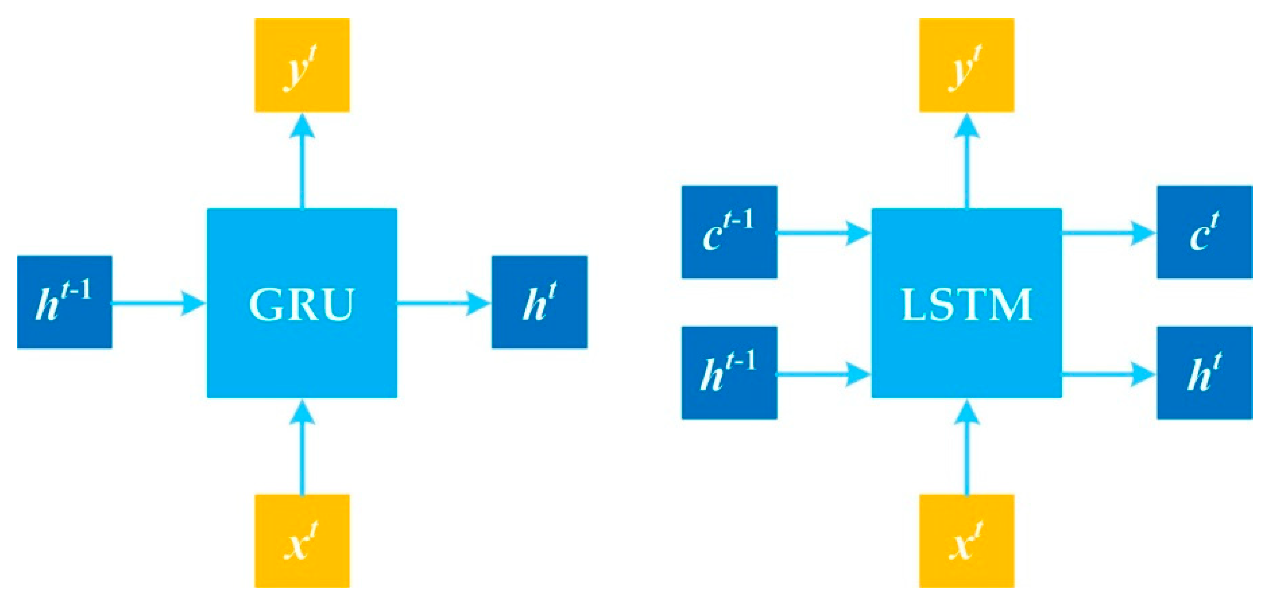
Long Short-Term Memory [68] (LSTM) is a special type of Recurrent Neural Network (RNN) that can prevent gradient vanishing and exploding in the course of long-sequence training. Even though LSTM is widely used, it nevertheless has many parameters, which makes training more difficult. Compared with traditional RNN, LSTM applies the gating mechanism to memorize past information and selectively forget some unimportant information. Three gating signals, the input gate, the forget gate, and the output gate, are constructed to realize the above-mentioned gating mechanism. Therefore, each input vector needs to be mapped into four signals before being input into the cell, corresponding to the input gate, forget gate, output gate, and input vector, respectively. Consequently, the LSTM model will expand by about four times the number of parameters. GRU optimizes the gating mechanism based on LSTM. It uses only two gates, reset gate and update gate, to achieve the same function. It is computationally cheaper and reduces the problem of gradient disappearance while maintaining the same performance. Therefore, GRU is selected as part of the real-time risk assessment model in this paper. Figure 4 depicts the primary structural differences between the GRU and LSTM.
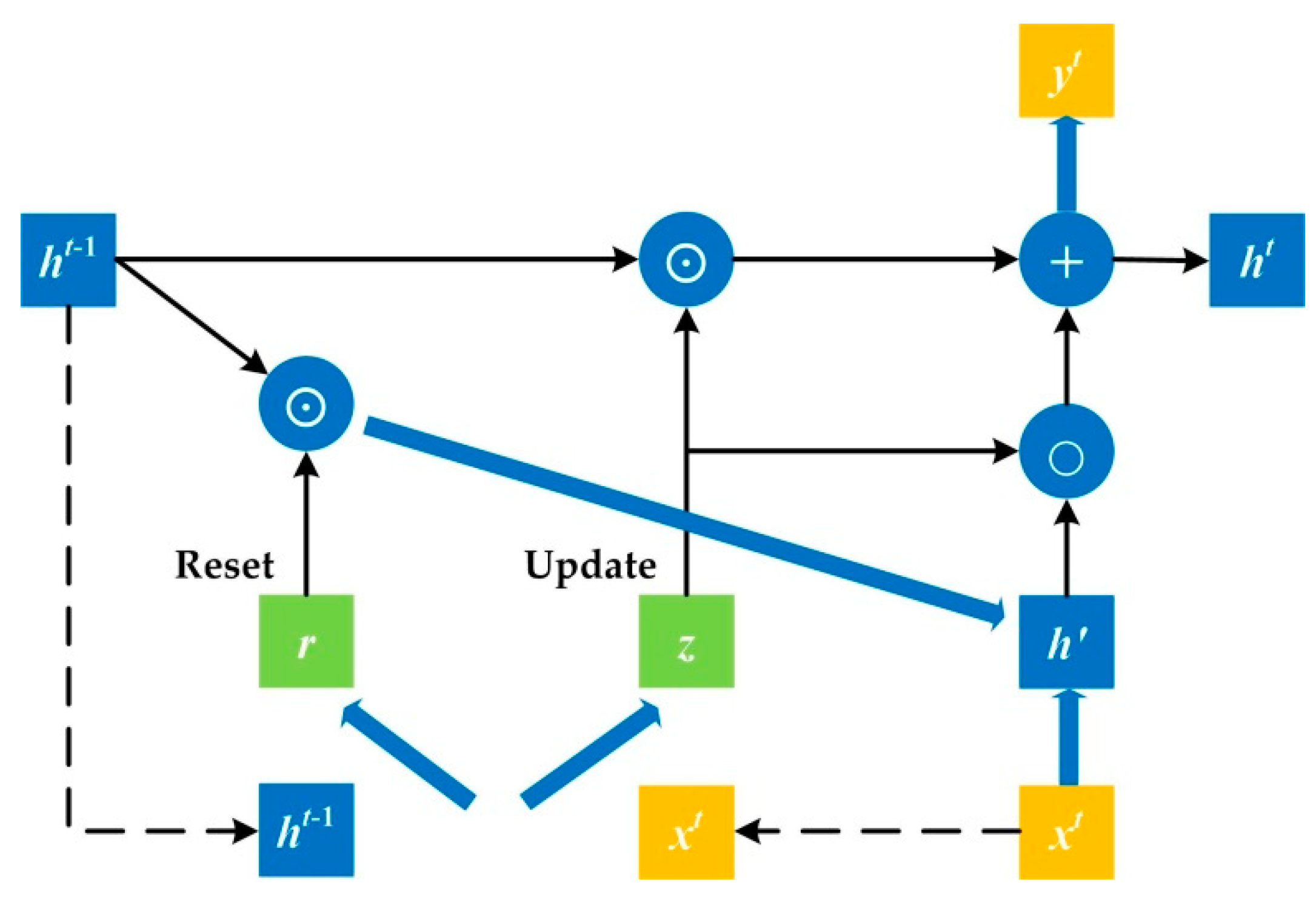
The GRU obtains the two gated states from the transmitted state h t 1 and the input x t of the current node. These two gated states are used to control both the reset gated state r and the update gated state z , as shown in Figure 5, below.
Firstly, the reset gate signal was obtained by the current memory value h t 1 and input vector x t , as shown in Equation (3). Among them, the σ ( x ) refers to the sigma non-linear function. After obtaining the gated signal, we reset the gated state r t to obtain the memory value after updating h t . This first resets the existing memory h t 1   and then stitches it with the current input x t . The transformed value is then applied with an activation transform to scale the data to a range of −1~1, as presented in Equation (4). As a result, h t is obtained, as shown in Figure 4. In this way, h t is targeted to add to the current hidden state, i.e., the state at the current moment is memorized.
r t = σ ( W r · [ h t 1 , x t ] )
h t = tan h ( W h · [ r t · h t 1 , x t ] )
In the updating phase, first the update gate signal is acquired by the same means as Equation (5). Then, GRU uses the same gated z to forget and remember at the same time, and the update expression is as Equation (6).
z t = σ ( W z · [ h t 1 , x t ] )
h t = ( 1 z ) h t 1 + z h t
The range of z is [0, 1]. The closer z is to 1, the greater the amount of data that is remembered; the closer to 0, the more that is forgotten.

2.3.2. DNN Model

DNN can be described as a series of associations between functional transformations and models, as shown in Figure 6. The inputs X = { x 1 , , x i , , x n } ( n = 20 ) by the first network layer are the real-time contributing factors to risk of hazmat road transportation, and we have
a i = b i + i = 1 n x i w i
where a i , b i and w i are defined as the activation, bias, and model weights, respectively. z 1 , , z j , , z m are defined as the units of hidden layer Z , and are obtained via activation function, as presented in Equation (8).
z j = g ( a i )
The most commonly used activation function g ( · ) is the sigmoid. There can be multiple hidden layers. Figure 6 shows only one hidden layer for the sake of simplicity. The activation of the output layer, a 0 , is given by the combination of hidden units, as follows.
a 0 = b 0 + j = 1 m z j w 0 , j
where a 0 , b 0 and w 0 , j are the activation, bias, and model weights, respectively. Finally, the activation function h ( · ) is used to obtain the output Y = { y 1 , y 2 , y 3 , y 4 } , which represents the risk of level IV (blue), level III (green), level II (yellow) and level I (red), as shown in Table 1 and Figure 7.
Y = h ( a 0 )
Given a contributing factor dataset X and associated risk set Y , a model is trained while minimizing the loss function, such that a new input X is able to predict Y in real time. Figure 7 presents the framework for risk assessment based on the DNN model.

3. Experiment and Analysis

3.1. Data Preliminary

The data were mainly obtained from the records in Shaanxi RTA and Shaanxi TMC in China. In accordance with the risk classification and contributing factors for hazmat road transportation described in Section 2.1, we established a hazmat road transportation database, and 2100 samples of data were selected as experimental data.
Two datasets were created from the entire hazmat road transportation database. One was the training set, with 2/3 of X = { x 1 , , x i , , x 20 } and corresponding Y = { y 1 , y 2 , y 3 , y 4 } , and the other was the validation set, with 1/3 of X = { x 1 , , x i , , x 20 } and corresponding Y = { y 1 , y 2 , y 3 , y 4 } . The classifier used in this paper was tf.contrib.learn. The GRU-DNN model with MFE used DNNClassifier from the open-source library TensorFlow.

3.2. Performance Meausures

For the input data, there are four different recognition states following model prediction: True Positives (TP), False Positives (FP), True Negatives (TN) and False Negatives (FN). The specific meanings for these recognition states are provided in Table 3. The output labels are compared with the ground truth. When a correct prediction is made, the number of correct predictions incremented by 1 and the proportion of corresponding recognition state is changed. When a wrong prediction is made, the number of wrong predictions is incremented by 1 and the proportion of corresponding recognition state is changed.
In this paper, four prevalent performance measures were selected to evaluate the model, including accuracy (ACC), precision (PR), recall (RE), and F1-score (F1). The derivations and definitions of the performance measures are demonstrated in Table 4.

3.3. Model Training

For the real-time risk assessment model of hazmat road transportation based on GRU-DNN with MFE, the cross-entropy cost function was used as the loss function, as presented in Equation (11).
l ( W ) = k = 1 s [ ( 1 Y ( k ) ) log ( 1 Y ^ ( X ( k ) ) ) + Y ( k ) log Y ^ ( X ( k ) ) ] +   min λ 2 W 2
where s denotes the number of samples. Y ^ ( X ( k ) ) is the predicted value of the sample X ( k ) . ( X ( k ) , Y ( k ) ) represents the data samples and corresponding labels. The second term is the weight penalty term, and λ is the penalty coefficient.
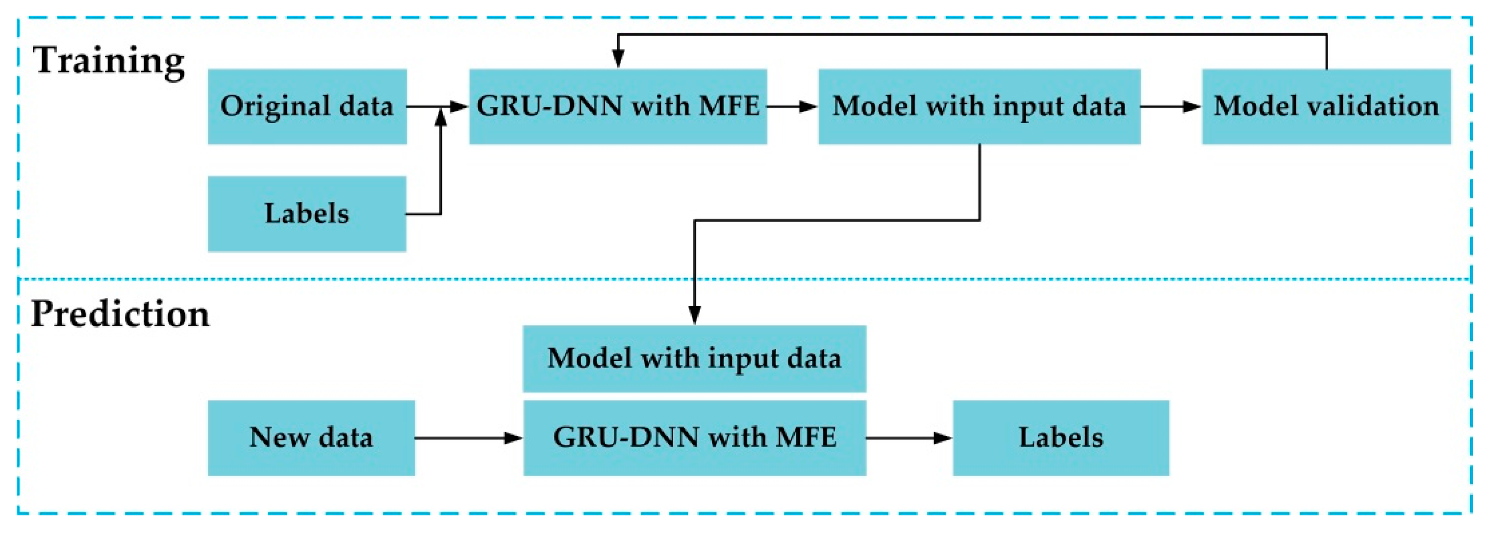
During model building, we added dropout and batch normalization (BN) operators to prevent model overfitting. The dropout operator allows the model to stop the activation of a neuron with a certain probability during forward propagation. This makes the model more generalizable, because it does not depend too much on some local features. The BN operation is added between each layer of the CNN, which can adjust the weights of neurons to a standard normal distribution. Generally speaking, with increasing network depth, the model becomes more difficult to train and the convergence becomes slower and slower. Through the adjustment of the BN layer, the input of each layer can be unified to a fixed distribution. In this way, the complexity of the model can be appropriately increased to prevent the model from overfitting. Adam was chosen as the optimizer of the model. The learning rate was set as 0.001, and the mini-batch was 10. To improve the computational efficiency and smooth the output curve for comparative analysis, the average loss was recorded for every 10 epochs and the trained model was verified and saved for every epoch. Therefore, the training results of different stages were analyzed. In Figure 8, the training procedure is displayed.
To evaluate the impact of different learning rates on the GRU-DNN with MFE, three learning rates of 0.002, 0.001 and 0.0001 were set in the training process based on the transfer learning strategy [69]. The losses with different learning rate are presented in Figure 9.
Figure 9 indicates that the loss of the learning rate 0.001 is the lowest. The training loss decreased rapidly in the first 200 epochs, and the training tended to stabilize after 400 epochs. To evaluate the performance of the model, the four measures described above were used, as demonstrated in Table 5.
Actually, in addition to ACC, PR and RE should also be considered. The former shows the proportion of accurate predictions made by the model among all the predicted samples. The latter shows the proportion of predicted positive samples to the true samples. In the prediction of an emergency, such as accidents during hazmat road transportation, consideration should not only be of FPs and TPs, but rather the RE should also be used as a measure. Therefore, the model offers great prediction performance.
Then, we compared performance between the training sets and validation sets. The ACCs of the TS and VS with a learning rate of 0.001 are shown in Figure 10.
As illustrated in Figure 10, the average ACC of the model on the training sets reaches up to 93.51%, and it reaches 87.6% on the validation set. Combined with the RE shown in Table 5, the model has excellent performance in real-time risk assessment of hazmat road transportation. Table 6 shows the prediction results of three real-time risk levels. The road transportation accidents corresponding to the three real-time risk levels are fatal accidents, injury accidents, and property damage accidents. Their ACCs are 94.3%, 95.8%, and 90.5%, respectively. Among them, the prediction of injury accidents is the most accurate, followed by fatal accidents. The results represent good performance of the model for the real-time risk assessment of hazmat road transportation, which meets the requirements of the experiments.

3.4. Model Comparison

In this section, models such as DNN, Convolutional Neural Network (CNN) [70], and Mixed Logistic Regression (MLR) [71] were integrated with MFE and applied to the same hazmat transportation dataset to serve as comparisons for GRU-DNN with MFE. ACC was selected as the performance measure. The ACCs of DNN with MFE, CNN with MFE, MLR with MFE and GRU-DNN with MFE are illustrated in Figure 11.
As shown in Figure 11, the curves were fitted according to the results such that they became smoother and easier to interpret. The GRU-DNN with MFE converges better than the other three models. It has better performance and generalization ability. Figure 12 is the PR-RE (P-R) curve of the model of GRU-DNN with MFE. This curve completely covers the P-R curves of the other three models, indicating that the GRU-DNN with MFE offers the best performance among the four models.
This study also applied the following models to the prediction of the real-time risk of hazmat road transportation to serve as comparisons with our model: K-Nearest Neighbor (KNN) [72], Support Vector Machine (SVM) [73], Naive Bayes (NB) [74], Decision Tree (DT) [75], and Random Forest (RF) [64]. MFE was integrated with these models as well. A performance comparison of the nine models is presented in Table 7. AUC is the area under the receiver operating characteristic (ROC) curve 7 [76]. If the ROC curve of a model encircles that of another one, the former model is definitely better than the latter one. However, AUC is more appropriate for the comparison among models if the ROCs of these models intersect with each other. AUC values often fall between 0.5 and 1. The closer the AUC gets to 1.0, the more accurately the model captures reality. When it is equal to 0.5, the model only poorly reflects reality reality.
Even though the ACCs of CNN, KNN and RF with MFE are slightly higher than that of GRU-DNN with MFE, the AUC of GRU-DNN is significantly higher than that of the other three models. After the analysis of ACC, AUC and F1, presented in Table 7, the performance of GRU-DNN with MFE was found to be better than that of any of the other models on the basis of the comparison in this paper.

4. Adversarial Attack and Defenses

During the road transportation of hazmat, some errors in risk assessment or emergency rescue decision making can potentially lead to major accidents. The effectiveness of deep learning cannot be guaranteed when the dataset contains noise, errors and so forth. In particular, for the hazmat road transportation accident dataset, the sample size is relatively small, such that the results are likely to be biased and sensitive to noise and error. Therefore, it is necessary to improve the robustness of the GRU-DNN with MFE, reducing the number of false warnings caused by abnormal feedback data.
Adversarial attacks are widely used in deep learning. Given an input, an adversarial attack tries to produce a perturbation or distortion to the input leading the input to be misclassified by a well-trained DNN. The antagonistic case must typically be misclassified with high confidence. Widely used adversarial attacks include FGSM [48], JSMA [49], DeepFool [50], C&W attack [51], etc. C&W attack was developed based on FGSM and transforms the generation of adversarial examples into a constrained optimization problem, minimizing the l 0 -, l 2 - or l -norm-based perturbations under the premise that the model outputs are all wrong results. Additionally, the formulation of the C&W attack can avoid the box constraint. The C&W attack is regarded as being a powerful attack that is more effective than FGSM, JSMA and DeepFool. It is able to generate an adversarial example that has a significantly smaller perturbation distance, especially on the l 2 -norm metric [46].
In this paper, C&W attack with l 2 -norm mode was performed, using the following constrained optimization problem.
minimize δ 2 + c max { max i l ( Z ( X + δ ) i ) Z ( X + δ ) t , κ }
subject   to   X + δ [ 0 , 1 ] n
where δ denotes the adversarial perturbations and δ = { δ 1 , , δ n } where n = 20 in this paper. δ 2 is the l 2 -norm and δ 2 = ( i = 1 n δ i 2 ) 1 2 . Z ( · ) denotes the hidden layer of the proposed model. t and l are the target and correct labels of X , respectively. κ represents the confidence that the adversarial example is misclassified. The higher the κ , the stronger the attack ability, but the larger the perturbations of the adversarial example. The first term in Equation (7) represents the distance between normal sample X and adversarial example X + δ . The objective is to find a small change from δ to X such that the classification of X is changed, but the result is still valid, which is reflected by the second term. The main part of the second term should have been in the constraint condition. Due to its high non-linearity and box characteristic, it is added to the objective function for optimization with a hyperparameter c , balancing the weight of the two terms and avoiding the box constraint.
On the opposite side of adversarial attacks, various defense techniques have been developed that aim to either provide immunity from the attack or to identify the adversarial examples such that the decision of the DNN will be more robust. The evolution of attack and defense strategies has previously been presented as an “arms race”. For example, most defenses against attacks in white box settings, such as defensive distillation [55], have been demonstrated to be vulnerable to attacks relying on iterative optimization, as is the case with the C & W attack [51,77].
In this study, we perform and compare three approaches for adversarial defenses: adversarial training [48,52], dimensionality reduction [53], and prediction similarity [54].

4.1. Adversarial Training

Among the most notable forms of defense is adversarial training. By retraining the model using adversarial examples and learning to classify them correctly, it is possible to increase the resilience of DNNs against adversarial attacks. Its principle can be expressed as follows:
θ * = argmin θ E ( X , Y ) T [ max δ [ ϵ , ϵ ] n l ( X + δ ; Y ; f θ ) ]
where f θ is GRU-DNN parameterized by θ . l ( · ) denotes the loss function. T is the training set. E represents the probabilistic expectation. This expression is based on the assumption that all neighbors within the allowed perturbation ball [ ϵ , ϵ ] n should have the same class label, i.e., local robustness.

4.2. Dimensionality Reduction

Techniques for dimensional reduction aim to project high-dimensional data into a lower-dimensional space under certain constraints. When dealing with high-dimensional data, i.e., each sample comprises a lot of features, it is challenging to determine which characteristics are crucial. Imposing constraints may also make the performance of learning tasks on the data in the original high-dimensional space problematic. Before the data are processed as input to the DNN in dimensionality reduction cases, the data are projected onto a lower-dimensional space first, which removes as much noise as possible and makes the classifier more robust via modifying the training phase.
Due to the structural characteristics of GRU-DNN, the dimensionality reduction layer, presented as encoder or autoencoder, can be inserted in different positions, as presented in Figure 13.
The first dimensionality reduction method is the intermediate encoder. The intermediate encoder is used to obtain variables between the initial GRU and the new DNN. The new DNN is trained with the output of the encoder as the input data. This defense differs from other defenses because the encoder trains a new DNN, leading the structure of the GRU-DNN model to change. It reduces the dimensionality of the DNN features and eliminates the least important features to denoise.
The second method is the intermediate autoencoder. It will be inserted into the DNN previously. In this case, the GRU-DNN-based model is not retrained, with the GRU and DNN retaining their original structures. The intermediate autoencoder denoises the output of the GRU before the GRU output is used as the input data for the DNN.
The last is the initial autoencoder which uses the dataset to train the autoencoder and inserts it before the GRU. Both GRU and DNN remain the original weights and are not retrained. The initial autoencoder cleans up the data noise after MFE and before the GRU-DNN which is used to make classifications.

4.3. Prediction Similarity

Prediction similarity does not modify the model directly, being an external layer added to the original model. This external layer saves the history records of input, assessment output, and specifically designed features. The premise is the inspiration behind the features that adversarial assaults require several assessments of comparable data to produce adversarial examples. Based on the data obtained in the external layer, a probability assessment feature can be generated to evaluate whether the input is adversarial or not. To compare the real input data with prior data, similarity metrics are used. This layer could take a step to fend off the adversarial attack if it is highly probable that the output of the layer would serve as the real sample in an adversarial example.
Contributing factors, predicted risk assessment value (the level and the probability), minimum distance to all previous samples, prediction alarm (number of times the percentage of the class is smaller) and distance alarm (number of samples with distance less than the threshold) are selected as the features saved in each prediction. The similarity between two samples is measured by mean squared error (MSE)
When an attack is identified, action is taken to stop it. In this paper, it returns the opposite class if the detector senses something suspicious. This causes the adversarial attack to believe that it has already achieved an adversarial example, when it actually has not.

4.4. Effectiveness of the Three Defense Approaches

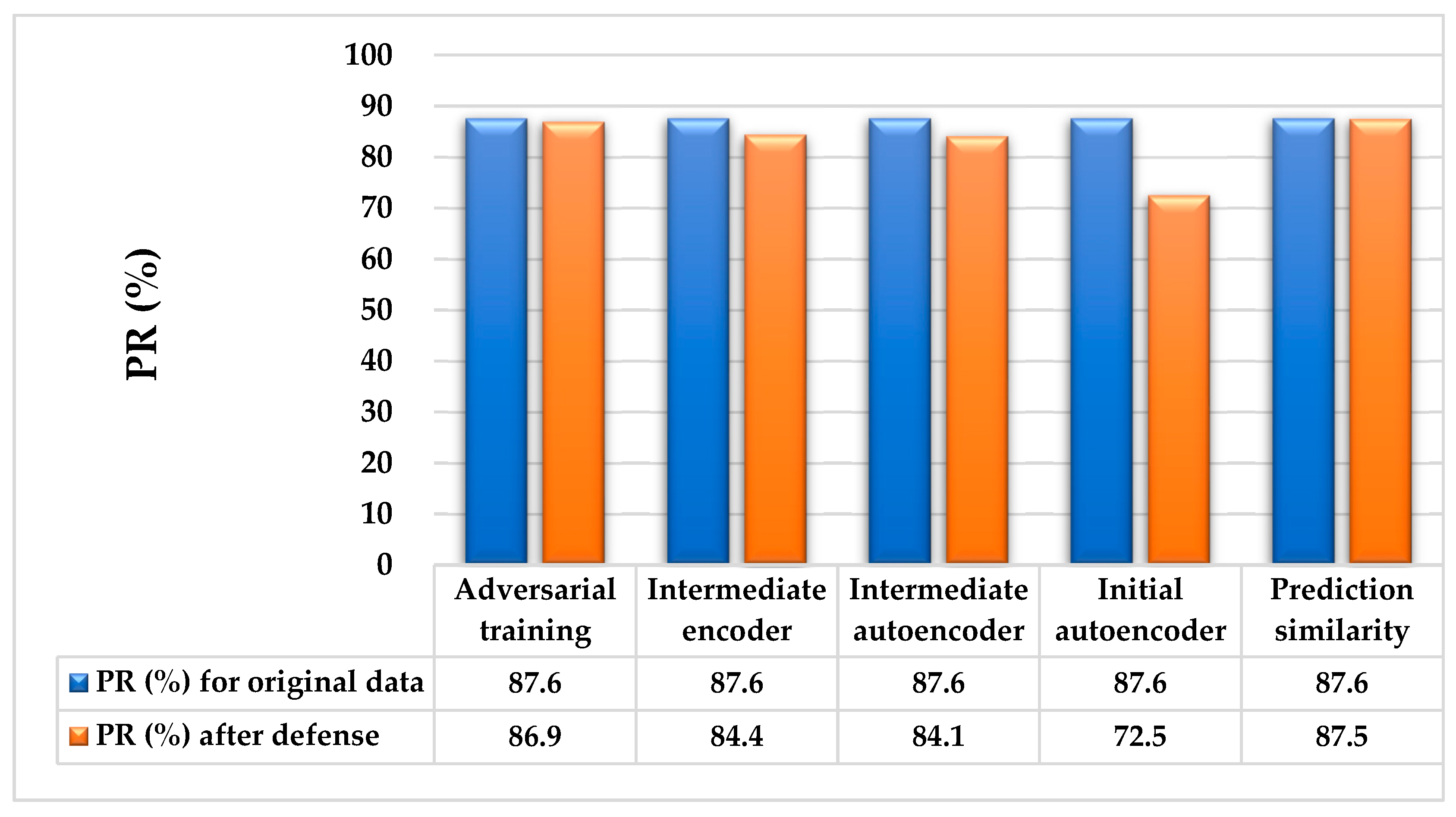
Compared with the original model, GRU-DNN with MFE, PRs of the defense GRU-DNN with MFE via adversarial training and dimensionality reduction both decrease, as shown in Figure 14. The prediction similarity method detects adversarial attacks and returns the opposite class, for example, FP. This may affect the PR of the model. However, it can be seen from the experimental results in Figure 13 that the defense of GRU-DNN with MFE via prediction similarity and the original model leave little gap in PR. The PR of the prediction similarity is the closest to the original GRU-DNN with MFE among the three approaches.
Additionally, the impacts of known and new adversarial attacks on the three defense approaches are investigated, as shown in Table 8. Adversarial training is the best option to differentiate among known adversarial examples. Unfortunately, if there are new adversarial attacks, it is unable to detect new adversarial attack attempts. In this case, adversarial training is therefore unreliable. For dimensionality reduction, even though it does not detect new adversarial attacks, new adversarial attacks are nevertheless distinguishable from known attacks to human eyes. Unlike the former two approaches, prediction similarity is capable of detecting new adversarial attacks with a success rate of 99.5%, which is obviously the highest among the three approaches.
In sum, for adversarial training, dimensionality reduction and prediction similarity to improve the robustness of the GRU-DNN with MFE, the following conclusions can be drawn:
(1)
Adversarial training increases the difficulty of generating new adversarial attacks. With the new adversarial examples obtained, the model has to be retrained to ensure those vulnerabilities are taken into consideration, which is an infinite recursive defense process.
(2)
Dimensionality reduction is effective at seeking new vulnerabilities, since the generation of new adversarial examples is detectable to the human eye. When PR remains stable, the GRU-DNN with MFE can be made more robust.
(3)
Prediction similarity is only the addition of an external detection layer and does not necessitate the modification of the structure of GRU-DNN with MFE, such that the known adversarial examples are impossible to detect using this approach. However, it can be used as an effective input for risk assessment to detect with a high success rate when an adversarial attack is launched, thus significantly improving the robustness of the model.

5. Conclusions

To assess the real-time risk of hazmat road transportation based on various types of data for contributing factors, this paper developed a gated recurrent unit-deep neural network (GRU-DNN) model integrated with multimodal feature embedding (MFE). MFE was incorporated into the framework of the deep learning model, in which discrete variables, continuous variables, and images were uniformly embedded. GRU was a pre-trained sub-model, the relative structure and weight of which could subsequently be used directly by the DNN, improving the poor classification and recognition results due to the insufficient number of samples. Then, the model was trained and validated based on a hazmat road transportation database of 2100 samples with 20 real-time contributing factors and four risk levels. Furthermore, the performance measures were evaluated in the numerical examples, whereby the accuracies (ACCs), precisions (PRs), recalls (REs), F1-scores (F1s) and areas under receiver-operating-characteristic curves (AUCs) were compared between the proposed model and other widely used models. Finally, Carlini & Wagner attack and three corresponding defenses—adversarial training, dimensionality reduction and prediction similarity—were proposed in the training to improve the robustness of the model, alleviating the impact of noise and error on the small-sized samples.
The results demonstrated that the average ACC of the model was able to reach 93.51% and 87.6% on the training and validation sets, respectively. The prediction of injury accidents was the most accurate, followed by fatal accidents. Combined with the 89.0% RE, the model demonstrated excellent performance at real-time risk assessment of hazmat road transportation. In addition, the proposed model outperformed DNN, Convolutional Neural Network, Mixed Logistic Regression, K-Nearest Neighbor, Support Vector Machine, Naive Bayes, Decision Tree, and Random Forest based on the overall comparisons of the ACC, AUC, F1 and PR-RE curve. Finally, prediction similarity was an effective approach for improving the robustness of GRU-DNN with MFE, with the launched adversarial attacks being detected with a high success rate.
In future research, more variables will be considered. Meanwhile, multimodal data fusion will adopt more fusion methods to better analyze the state of road transportation of hazardous materials. On the other hand, data on the road transportation of hazardous materials is insufficient. Therefore, more robust prediction models are needed for small numbers of samples. At the same time, during the model deployment process, the mechanism of continuously updating the model based on the difference between the predicted data and the real data should also be explored in the future.

Author Contributions

Conceptualization, S.Y. and Y.L. (Yi Li); methodology, S.Y., Y.L. (Yishun Li) and Y.L. (Yi Li); software, Y.L. (Yishun Li); validation, Y.L. (Yi Li); formal analysis, Y.L. (Yi Li); investigation, S.Y. and G.L.; resources, G.L.; data curation, Y.L. (Yishun Li); writing—original draft preparation, S.Y., Y.L. (Yi Li) and Z.X.; writing—review and editing, S.Y. and Y.L. (Yishun Li); visualization, S.Y.; supervision, Y.L. (Yi Li); project administration, S.Y.; funding acquisition, S.Y. All authors have read and agreed to the published version of the manuscript.

Funding

This research was funded by National Natural Science Foundation of China, grant number 71901190 and Project for Science and Technology Plan of Guangxi, China, grant number AB20159032.

Institutional Review Board Statement

Not applicable.

Data Availability Statement

The data presented in this study are available on request from the corresponding author.

Conflicts of Interest

The authors declare no conflict of interest.

References

  1. Liu, L.; Wu, Q.; Li, S.; Li, Y.; Fan, T. Risk assessment of hazmat road transportation considering environmental risk under time-varying conditions. Int. J. Environ. Res. Public Health 2021, 18, 9780. [Google Scholar] [CrossRef] [PubMed]
  2. Dong, S.; Zhou, J.; Ma, C. Design of a network optimization platform for the multivehicle transportation of hazardous materials. Int. J. Environ. Res. Public Health 2020, 17, 1104. [Google Scholar] [CrossRef] [Green Version]
  3. Li, Y.; Xu, D.; Shuai, J. Real-time risk analysis of road tanker containing flammable liquid based on fuzzy Bayesian network. Process Saf. Environ. Prot. 2020, 134, 36–46. [Google Scholar] [CrossRef]
  4. Ditta, A.; Figueroa, O.; Galindo, G.; Yie-Pinedo, R. A review on research in transportation of hazardous materials. Socio-Econ. Plan. Sci. 2019, 68, 100665. [Google Scholar] [CrossRef]
  5. Guo, J.; Luo, C. Risk assessment of hazardous materials transportation: A review of research progress in the last thirty years. J. Traffic Transp. Eng. Engl. Ed. 2022, 9, 571–590. [Google Scholar] [CrossRef]
  6. Erkut, E.; Tjandra, S.; Verter, V. Hazardous materials transportation. Handb. Oper. Res. Manag. Sci. 2007, 14, 539–621. [Google Scholar]
  7. Huang, X.; Wang, X.; Pei, J.; Xu, M.; Huang, X.; Luo, Y. Risk assessment of the areas along the highway due to hazardous material transportation accidents. Nat. Hazards 2018, 93, 1181–1202. [Google Scholar] [CrossRef]
  8. Liu, X.; Turla, T.; Zhang, Z. Accident-cause-specific risk analysis of rail transport of hazardous materials. Transp. Res. Rec. J. Transp. Res. Board 2018, 2672, 176–187. [Google Scholar] [CrossRef]
  9. Ma, C.; Zhou, J.; Xu, X.; Pan, F.; Xu, J. Fleet scheduling optimization of hazardous materials transportation: A literature review. J. Adv. Transp. 2020, 2020, 4079617. [Google Scholar] [CrossRef]
  10. Gaweesh, S.; Khan, M.; Ahmed, M. Development of a novel framework for hazardous materials placard recognition system to conduct commodity flow studies using artificial intelligence AlexNet Convolutional Neural Network. Transp. Res. Rec. J. Transp. Res. Board 2021, 2675, 1357–1371. [Google Scholar] [CrossRef]
  11. Li, S.; Zu, Y.; Fang, H.; Liu, L.; Fan, T. Design optimization of a HAZMAT multimodal Hub-and-Spoke network with detour. Int. J. Environ. Res. Public Health 2021, 18, 12470. [Google Scholar] [CrossRef] [PubMed]
  12. Hu, H.; Li, X.; Zhang, Y.; Shang, C.; Zhang, S. Multi-objective location-routing model for hazardous material logistics with traffic restriction constraint in inter-city roads. Comput. Ind. Eng. 2019, 128, 861–876. [Google Scholar] [CrossRef]
  13. Zero, L.; Bersani, C.; Paolucci, M.; Sacile, R. Two new approaches for the bi-objective shortest path with a fuzzy objective applied to HAZMAT transportation. J. Hazard. Mater. 2019, 375, 96–106. [Google Scholar] [CrossRef] [PubMed]
  14. Zhong, H.; Wang, J.; Yip, T.; Gu, Y. An innovative gravity-based approach to assess vulnerability of a Hazmat road transportation network: A case study of Guangzhou, China. Transp. Res. Part D Transp. Environ. 2018, 62, 659–671. [Google Scholar] [CrossRef]
  15. Li, Y.; Yang, Q.; Chin, K. A decision support model for risk management of hazardous materials road transportation based on quality function deployment. Transp. Res. Part D Transp. Environ. 2019, 74, 154–173. [Google Scholar] [CrossRef]
  16. Hu, H.; Du, J.; Li, X.; Shang, C.; Shen, Q. Risk models for hazardous material transportation subject to weight variation considerations. IEEE Trans. Fuzzy Syst. 2020, 29, 2997467. [Google Scholar] [CrossRef]
  17. Zhou, L.; Guo, C.; Cui, Y.; Wu, J.; Lv, Y.; Du, Z. Characteristics, cause, and severity analysis for hazmat transportation risk management. Int. J. Environ. Res. Public Health 2020, 17, 2793. [Google Scholar] [CrossRef] [Green Version]
  18. Arun, A.; Haque, M.; Bhaskar, A.; Washington, S.; Sayed, T. A systematic mapping review of surrogate safety assessment using traffic conflict techniques. Accid. Anal. Prev. 2021, 153, 106016. [Google Scholar] [CrossRef]
  19. Cordeiro, F.; Bezerra, B.; Peixoto, A.; Ramos, R. Methodological aspects for modeling the environmental risk of transporting hazardous materials by road. Transp. Res. Part D Transp. Environ. 2016, 44, 105–121. [Google Scholar] [CrossRef]
  20. Janno, J.; Koppel, O. Operational risks in dangerous goods transportation chain on roads. LogForum 2018, 14, 33–41. [Google Scholar] [CrossRef]
  21. Verter, V.; Kara, B. A GIS-based framework for hazardous materials transport risk assessment. Risk Anal. 2001, 21, 1109–1120. [Google Scholar] [CrossRef] [PubMed]
  22. Ronza, A.; Vílchez, J.; Casal, J. Using transportation accident databases to investigate ignition and explosion probabilities of flammable spills. J. Hazard. Mater. 2007, 146, 106–123. [Google Scholar] [CrossRef]
  23. Landucci, G.; Antonioni, G.; Tugnoli, A.; Bonvicini, S.; Molag, M.; Cozzani, V. HazMat transportation risk assessment: A revisitation in the perspective of the Viareggio LPG accident. J. Loss Prev. Process Ind. 2017, 49, 36–46. [Google Scholar] [CrossRef]
  24. Benekos, I.; Diamantidis, D. On risk assessment and risk acceptance of dangerous goods transportation through road tunnels in Greece. Saf. Sci. 2017, 91, 1–10. [Google Scholar] [CrossRef]
  25. Ke, G.; Zhang, H.; Bookbinder, J. A dual toll policy for maintaining risk equity in hazardous materials transportation with fuzzy incident rate. Int. J. Prod. Econ. 2020, 227, 107650. [Google Scholar] [CrossRef]
  26. Tao, L.; Chen, L.; Long, P.; Chen, C.; Wang, J. Integrated risk assessment method for spent fuel road transportation accident under complex environment. Nucl. Eng. Technol. 2021, 53, 393–398. [Google Scholar] [CrossRef]
  27. Weng, J.; Gan, X.; Zhang, Z. A quantitative risk assessment model for evaluating hazmat transportation accident risk. Saf. Sci. 2021, 137, 105198. [Google Scholar] [CrossRef]
  28. Qu, Z.; Wang, Y. Research on risk assessment of hazardous freight road transportation based on BP neural network. Int. Conf. Logist. Syst. Intell. Manag. 2010, 2, 629–631. [Google Scholar]
  29. Li, P.; Abdel-Aty, M. A hybrid machine learning model for predicting real-time secondary crash likelihood. Accid. Anal. Prev. 2022, 165, 106504. [Google Scholar] [CrossRef] [PubMed]
  30. Islam, R.; Khan, F.; Venkatesan, R. Real time risk analysis of kick detection: Testing and validation. Reliab. Eng. Syst. Saf. 2017, 161, 25–37. [Google Scholar] [CrossRef]
  31. Fabiano, B.; Currò, F.; Reverberi, A.; Pastorino, R. Dangerous good transportation by road: From risk analysis to emergency planning. J. Loss Prev. Process Ind. 2005, 18, 403–413. [Google Scholar] [CrossRef]
  32. Yang, J.; Li, F.; Zhou, J.; Zhang, L.; Huang, L.; Bi, J. A survey on hazardous materials accidents during road transport in China from 2000 to 2008. J. Hazard. Mater. 2010, 184, 647–653. [Google Scholar] [CrossRef]
  33. Citro, L.; Gagliardi, R. Risk assessment of hydrocarbon release by pipeline. Chem. Eng. Trans. 2012, 28, 85–90. [Google Scholar]
  34. Shen, X.; Yan, Y.; Li, X.; Xie, C.; Wang, L. Analysis on tank truck accidents involved in road hazardous materials transportation in China. Traffic Inj. Prev. 2014, 15, 762–768. [Google Scholar] [CrossRef] [PubMed]
  35. Ambituuni, A.; Amezaga, J.; Werner, D. Risk assessment of petroleum product transportation by road: A framework for regulatory improvement. Saf. Sci. 2015, 79, 324–335. [Google Scholar] [CrossRef] [Green Version]
  36. Krizhevsky, A.; Sutskever, I.; Hinton, G. ImageNet classification with deep convolutional neural networks. Adv. Neural Inf. Process. Syst. 2012, 25, 1097–1105. [Google Scholar] [CrossRef] [Green Version]
  37. Ma, X.; Tao, Z.; Wang, Y.; Yu, H.; Wang, Y. Long short-term memory neural network for traffic speed prediction using remote microwave sensor data. Transp. Res. Part C Emerg. Technol. 2015, 54, 187–197. [Google Scholar] [CrossRef]
  38. Deng, L. Deep learning: From speech recognition to language and multimodal processing. APSIPA Trans. Signal Inf. Process. 2016, 5, 1–15. [Google Scholar] [CrossRef]
  39. Beam, A.; Kohane, I. Big data and machine learning in health care. J. Am. Med. Assoc. 2018, 319, 1317–1318. [Google Scholar] [CrossRef]
  40. Zhang, Y.; Wang, S.; Xia, K.; Jiang, Y.; Qian, P. Alzheimer’s disease multiclass diagnosis via multimodal neuroimaging embedding feature selection and fusion. Inf. Fusion 2021, 66, 170–183. [Google Scholar] [CrossRef]
  41. Chen, W.; Wang, W.; Liu, L.; Lew, M. New ideas and trends in deep multimodal content understanding: A review. Neurocomputing 2021, 426, 195–215. [Google Scholar] [CrossRef]
  42. Dasgupta, K.; Das, A.; Das, S.; Bhattacharya, U.; Yogamani, S. Spatio-contextual deep network based multimodal pedestrian detection for autonomous driving. IEEE Trans. Intell. Transp. Syst. 2022, 23, 15940. [Google Scholar] [CrossRef]
  43. Wang, S.; Guo, W. Sparse multigraph embedding for multimodal feature representation. IEEE Trans. Multimed. 2017, 19, 1454–1466. [Google Scholar] [CrossRef]
  44. Szegedy, C.; Zaremba, W.; Sutskever, I.; Bruna, J.; Erhan, D.; Goodfellow, I.; Fergus, R. Intriguing properties of neural networks. arXiv 2014, arXiv:1312.6199. [Google Scholar]
  45. Deng, Z.; Yang, X.; Xu, S.; Su, H.; Zhu, J. Libre: A practical Bayesian approach to adversarial detection. In Proceedings of the IEEE/CVF Conference on Computer Vision and Pattern Recognition, Nashville, TN, USA, 20–25 June 2021; IEEE: Manhattan, NY, USA, 2021; pp. 972–982. [Google Scholar]
  46. Huang, X.; Kroening, D.; Ruan, W.; Sharp, J.; Sun, Y.; Thoma, E.; Wu, M.; Yi, X. A survey of safety and trustworthiness of deep neural networks: Verification, testing, adversarial attack and defence, and interpretability. Comput. Sci. Rev. 2020, 37, 100270. [Google Scholar] [CrossRef]
  47. Zhang, X.; Wang, J.; Wang, T.; Jiang, R.; Xu, J.; Zhao, L. Robust feature learning for adversarial defense via hierarchical feature alignment. Inf. Sci. 2021, 560, 256–270. [Google Scholar] [CrossRef]
  48. Goodfellow, I.J.; Shlens, J.; Szegedy, C. Explaining and harnessing adversarial examples. arXiv 2014, arXiv:1412.6572. [Google Scholar]
  49. Papernot, N.; McDaniel, P.D.; Jha, S.; Fredrikson, M.; Berkay Celik, Z.; Swami, A. The limitations of deep learning in adversarial settings. In Proceedings of the 2016 IEEE European Symposium on Security and Privacy (EuroS & P), Saarbruecken, Germany, 21–24 March 2016; IEEE: Manhattan, NY, USA, 2016; pp. 372–387. [Google Scholar]
  50. Moosavi-Dezfooli, S.M.; Fawzi, A.; Frossard, P. Deepfool: A simple and accurate method to fool deep neural networks. In Proceedings of the IEEE Conference on Computer Vision and Pattern Recognition, Las Vegas, NV, USA, 27–30 June 2016; IEEE: Manhattan, NY, USA, 2016; pp. 2574–2582. [Google Scholar]
  51. Carlini, N.; Wagner, D. Adversarial examples are not easily detected: Bypassing ten detection methods. In Proceedings of the 10th ACM Workshop on Artificial Intelligence and Security, Dallas, TX, USA, 3 November 2017; ACM: New York, NY, USA, 2017; pp. 3–14. [Google Scholar]
  52. Madry, A.; Makelov, A.; Schmidt, L.; Tsipras, D.; Vladu, A. Towards deep learning models resistant to adversarial attacks. arXiv 2017, arXiv:1706.06083. [Google Scholar]
  53. Xu, W.; Evans, D.; Qi, Y. Feature squeezing: Detecting adversarial examples in deep neural networks. In Network and Distributed System Security Symposium (NDSS); The Internet Society: Singapore, 2018. [Google Scholar]
  54. Echeberria-Barrio, X.; Gil-Lerchundi, A.; Egana-Zubia, J.; Orduna-Urrutia, R. Understanding deep learning defenses against adversarial examples through visualizations for dynamic risk assessment. Neural Comput. Appl. 2022, 1–14. [Google Scholar] [CrossRef]
  55. Hinton, G.; Vinyals, O.; Dean, J. Distilling the knowledge in a neural network. arXiv 2015, arXiv:1503.02531. [Google Scholar]
  56. Meng, D.; Chen, H. Magnet: A two-pronged defense against adversarial examples. In ACM Conference on Computer and Communications Security; ACM: New York, NY, USA, 2017. [Google Scholar]
  57. Dhillon, G.S.; Azizzadenesheli, K.; Lipton, Z.C.; Bernstein, J.; Kossaifi, J.; Khanna, A.; Anandkumar, A. Stochastic activation pruning for robust adversarial defense. arXiv 2018, arXiv:1803.01442. [Google Scholar]
  58. Lu, Y.D. Research on Real-Time Risk Warning Method for Hazardous Materials Transportation by Road; China University of Geosciences: Beijing, China, 2018. [Google Scholar]
  59. Wang, Q.; Si, G.; Qu, K.; Gong, J.; Cui, L. Transmission line foreign body fault detection using multi-feature fusion based on modified YOLOv5. J. Phys. Conf. Ser. 2022, 2320, 012028. [Google Scholar] [CrossRef]
  60. Wang, Z.; She, Q.; Smolic, A. ACTION-Net: Multipath excitation for action recognition. arXiv 2021, arXiv:2103.07372. [Google Scholar] [CrossRef]
  61. Abtahi, S.; Omidyeganeh, M.; Shirmohammadi, S.; Hariri, B. YawDD: A yawning detection dataset. In Proceedings of the 5th ACM Multimedia Systems Conference, Singapore, 19–21 March 2014; pp. 24–28. [Google Scholar]
  62. Howard, A.; Sandler, M.; Chu, G.; Chen, B.; Tan, M.; Wang, W.; Zhu, Y.; Pang, R.; Vasudevan, V. Searching for MobileNetV3. In Proceedings of the IEEE/CVF International Conference on Computer Vision, Seoul, Korea, 27 October–2 November 2019; IEEE: Manhattan, NY, USA, 2019; pp. 1314–1324. [Google Scholar]
  63. Kusner, M.J.; Paige, B.; Hernández-Lobato, J.M. Grammar variational autoencoder. In Proceedings of the International Conference on Machine Learning, Sydney, Australia, 6–11 August, 2017; pp. 1945–1954. [Google Scholar]
  64. Ham, J.; Chen, Y.; Crawford, M. Investigation of the random forest framework for classification of hyperspectral data. IEEE Trans. Geosci. Remote Sens. 2005, 43, 492–501. [Google Scholar] [CrossRef] [Green Version]
  65. Dey, R.; Saemt, F. Gate-variants of gated recurrent unit (GRU) neural networks. In Proceedings of the IEEE International Midwest Symposium on Circuits & Systems, Boston, MA, USA, 6–9 August 2017; IEEE: Manhattan, NY, USA, 2017; pp. 1597–1600. [Google Scholar]
  66. Diener, L.; Janke, M.; Schultz, T. Direct conversion from facial myoelectric signals to speech using Deep Neural Networks. In Proceedings of the 2015 International Joint Conference on Neural Networks (IJCNN), Killarney, Ireland, 12–17 July 2015. [Google Scholar]
  67. Li, Y.; Liu, C.; Yue, G.; Gao, Q.; Du, Y. Deep learning-based pavement subsurface distress detection via ground penetrating radar data. Autom. Constr. 2022, 142, 104516. [Google Scholar] [CrossRef]
  68. Shi, X.; Chen, Z.; Wang, H. Convolutional LSTM network: A machine learning approach for precipitation nowcasting. In Advances in Neural Information Processing Systems 28 (NIPS 2015); MIT Press: Cambridge, MA, USA, 2015. [Google Scholar]
  69. Li, Y.; Che, P.; Liu, C.; Wu, D.; Du, Y. Cross-scene pavement distress detection by a novel transfer learning framework. Comput. -Aided Civ. Infrastruct. Eng. 2021, 36, 1398–1415. [Google Scholar] [CrossRef]
  70. Li, B.; Wang, K.; Zhang, A. Automatic classification of pavement crack using deep convolutional neural network. Int. J. Pavement Eng. 2020, 21, 457–463. [Google Scholar] [CrossRef]
  71. Gai, K.; Zhu, X.; Li, H. Learning Piece-Wise Linear Models from Large Scale Data for Ad Click Prediction; Cornell University Library: Ithaca, NY, USA, 2017. [Google Scholar]
  72. Zhang, M.; Zhou, Z. ML-KNN: A lazy learning approach to multi-label learning. Pattern Recognit. 2007, 40, 2038–2048. [Google Scholar] [CrossRef]
  73. Hearst, M.; Dumais, S.; Osman, E. Support vector machines. IEEE Intell. Syst. Appl. 1998, 13, 18–28. [Google Scholar] [CrossRef] [Green Version]
  74. Chen, J.; Huang, H.; Tian, S. Feature selection for text classification with Naïve Bayes. Expert Syst. Appl. 2009, 36, 5432–5435. [Google Scholar] [CrossRef]
  75. Safavian, S.; Landgrebe, D. A survey of decision tree classifier methodology. IEEE Trans. Syst. Man Cybern. 1991, 21, 660–674. [Google Scholar] [CrossRef]
  76. Wang, Y.Y.; Chen, S.C. A survey of evaluation and design for AUC based classifier. Pattern Recognit. Artif. Intell. 2011, 24, 64–71. [Google Scholar]
  77. Carlini, N.; Wagner, D. Magnet and efficient defenses against adversarial attacks are not robust to adversarial examples. arXiv 2017, arXiv:1711.08478. [Google Scholar]
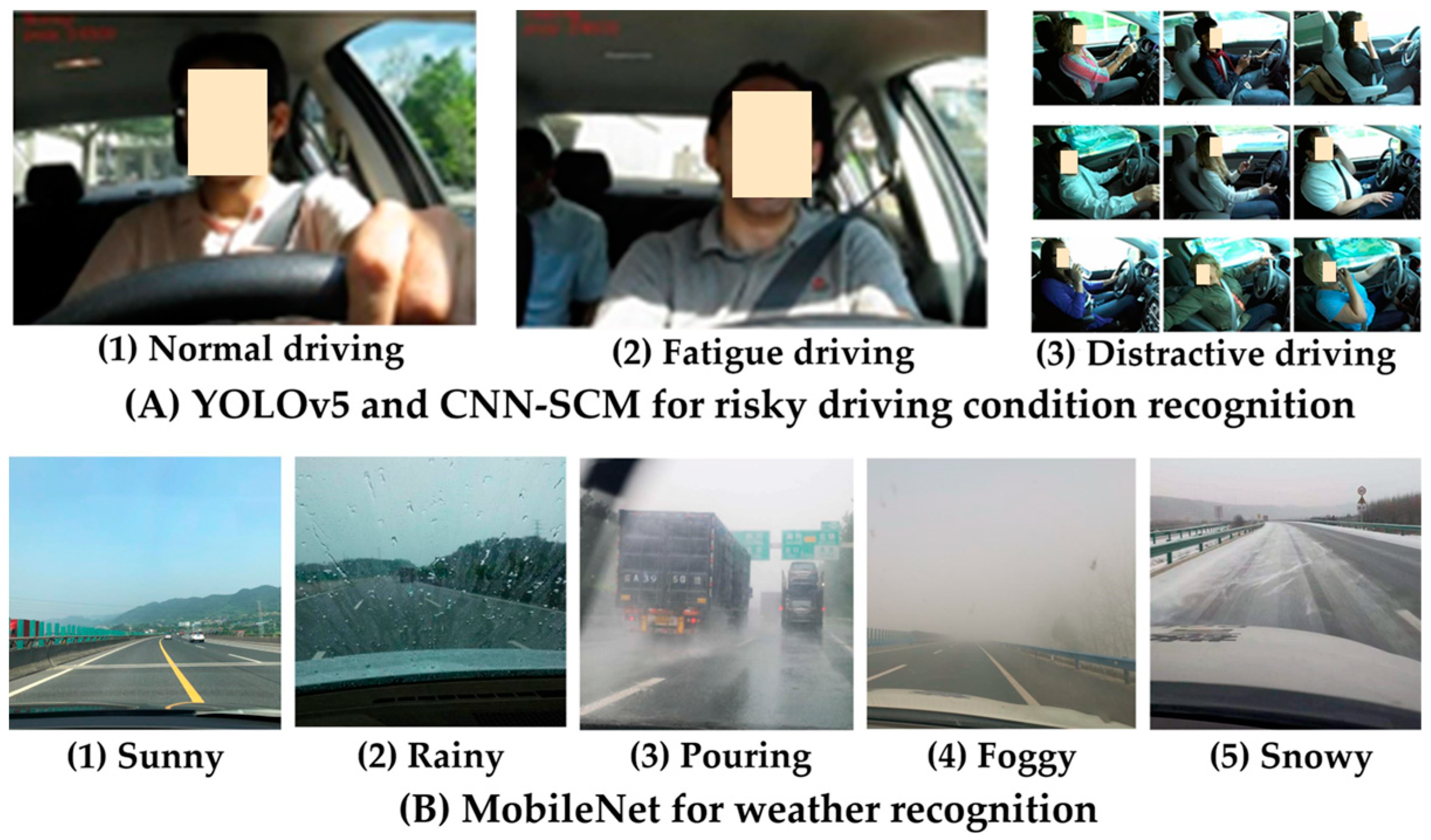
Figure 1. Recognitions for risky driving and weather conditions from dashboard camera.
Applsci 12 11130 g001
Figure 2. Multimodal feature embedding.
Applsci 12 11130 g002
Figure 3. Autoencoder for multimodal feature extraction.
Applsci 12 11130 g003
Figure 4. Structural comparison between GRU and LSTM.
Applsci 12 11130 g004
Figure 5. Gated information. (A) current gates state; (B) update gated state; (C) current transmitted state.
Applsci 12 11130 g005
Figure 6. Structure of GRU.
Applsci 12 11130 g006
Figure 7. Risk assessment based on DNN.
Applsci 12 11130 g007
Figure 8. Training process of GRU-DNN with MFE.
Applsci 12 11130 g008
Figure 9. Losses with different learning rates. (A) learning rate of 0.002; (B) learning rate of 0.001; (C) learning rate of 0.0001.
Applsci 12 11130 g009
Figure 10. ACCs of training and validation sets with 0.001 learning rate.
Applsci 12 11130 g010
Figure 11. ACCs of four models in training and validation sets. (A) training set; (B) validation set.
Applsci 12 11130 g011
Figure 12. P-R curves of four models.
Applsci 12 11130 g012
Figure 13. Dimensionality reduction encoders for GRU-DNN with MFE. (A) intermediate encoder; (B) intermediate autoencoder; (C) initial autoencoder.
Applsci 12 11130 g013
Figure 14. PR comparison between defense models and original model.
Applsci 12 11130 g014
Table 1. Real-time risk levels for hazmat road transportation.
Y LevelClassificationDescriptionColor for Presentation
1Level Iextremely high riskfatal accidentsred
2Level IIhigh riskinjury accidentsyellow
3Level IIImedium riskproperty damage accidentgreen
4Level IVlow riskno accidentblue
Table 2. Contributing factors for real-time risk of hazmat road transportation.
Attributes for Accident OccurrenceContributing Factor for AttributesType of DataValue of DataSource of Data
probabilitytravel speed of vehicle P 1 C[0, 120] (km/h)I
mileage of vehicle P 2 C[0, 4 × 10⁵] (km)I
inspection status of vehicle P 3 D0 = qualified
1 = disqualified
II
load of vehicle P 4 C0 = no overload
1 = overload
2 = heavy overload
VI
vehicle type P 5 D0 = tank
1 = van
III
accident-prone road section P 6 D0 = no accident-prone road section
1 = tunnel
2 = bridge
3 = long downgrade
4 = long upgrade
5 = zigzag
6 = village
7 = unsignalized intersection
IV and VII
risky driving condition P 7 Enormal, fatigue, distracted drivingV
traffic violation record P 8 D0 = no record
1 = traffic violation during transportation
2 = involved in normal accident
3 = involved in severe accident
III
duration for continuous driving P 9 C[0, 4] (h)IV
unsafe vehicle behavior P 10 D0 = no unsafe driving behavior
1 = unsafe car-following
2 = unsafe lane-changing
I or VI
time of the day P 11 D0 = morning
1 = noon
2 = afternoon
3 = night
4 = midnight
/
weather condition P 12 Esunny, raining, pouring, foggy, snowyV
severitytype of hazmat S 1 D0 = explosives
1 = compressed gases and liquefied gases
2 = flammable liquids
3 = flammable solids, substances liable to spontaneous combustion and substances emitting flammable gases when wet
4 = oxidizing substances and organic peroxides
5 = poisons and infectious substances
6 = radioactive substances
7 = corrosives
8 = miscellaneous dangerous substances
III
physicochemical property of hazmat S 2 D0 = explosive
1 = flammable
2 = corrosive
3 = oxidative
4 = poisonous
5 = radiative
III
ratio of hazmat amount to tank volume S 3 C[0, 92] (%)II
leakage of hazmat S 4 D0 = no leakage
1 = permeating leakage
2 = water-clock leakage
3 = heavy leakage
4 = flowing leakage
I and VI
social influencesensitive period I 1 D0 = no
1 = holiday
2 = festival
3 = other large-scale activities
/
traffic condition I 2 D0 = uncongested
1 = congested
2 = heavily congested
VI
vulnerable community passed by I 3 D0 = no vulnerable community
1 = school
2 = hospital
3 = large community
IV and VII
vulnerable natural region passed by I 4 D0 = no vulnerable natural region
1 = river
2 = reservoir or lake
3 = forest
IV and VII
Note: Type of data: C: continuous variable; D: discrete variable; E: image. Source of data: I: real-time sensors in vehicle; II: data transferred to RTA before transporting; III: database in RTA; IV: real-time GPS tracking; V: real-time dashboard camera; VI: real-time data in TMC; VII: data in GIS in RTA.
Table 3. Combination of labels and prediction results.
LabelAccidentNon-Accident
Prediction Result
AccidentTPFP
Non-accidentFNTN
Table 4. Derivations and definitions of four performance measures.
Performance MeasuresDerivationDefinition
ACC (%) T P + T N T P + T N + F P + F N Proportion of accurate predictions in the predicted sample
PR (%) T P T P + F P Proportion of true positives to predicted positives
RE (%) T P T P + T N Proportion of predicted positive samples to the true samples
F1 (%) 2 T P 2 T P + F P + F N Harmonic mean of precision and recall
Table 5. Performance of DRU-DNN with MFE.
MeasureACC (%)PR (%)RE (%)F1 (%)
Performance87.686.589.087.7
Table 6. Prediction result of real-time risk levels of road hazmat transportation.
Risk LevelPR (%)RE (%)F1 (%)
Risk level I94.383.288.4
Risk level II95.885.690.4
Risk level III90.582.586.3
Table 7. Comparisons among nine models.
ModelACC (%)AUCF1 (%)
GRU-DNN with MFE87.60.9187.7
CNN with MFE88.10.7783.6
MLR with MFE75.40.6267.1
DNN with MFE82.50.8178.1
KNN with MFE88.70.8288.3
SVM with MFE83.30.8081.5
NB with MFE76.90.8678.9
DT with MFE83.20.8583.3
RF with MFE88.80.8488.5
Table 8. Impacts of known and new adversarial attack on three defense approaches.
Defense ApproachesDetection for Known Adversarial AttackDetection of New Adversarial Attack
Adversarial training92.0%No new adversarial attack attempts are detected
Dimensionality reductionIntermediate encoder62.3%New adversarial attacks are not detected, but are known, and new attacks are distinguishable
Intermediate autoencoder65.3%
Initial autoencoder71.7%
Prediction similarity0%The detection rate of the new adversarial attacks is 99.5%
Publisher’s Note: MDPI stays neutral with regard to jurisdictional claims in published maps and institutional affiliations.