Article

GPR Data Augmentation Methods by Incorporating Domain Knowledge

1
Key Laboratory of Road and Traffic Engineering of the Ministry of Education, Tongji University, Shanghai 201804, China
2
Henan Wanli Transportation Technology Group Co., Ltd., Xuchang 461000, China
3
College of Resource and Environment, Henan Institute of Engineering, Zhengzhou 451191, China
*
Author to whom correspondence should be addressed.
Appl. Sci. 2022, 12(21), 10896; https://doi.org/10.3390/app122110896
Submission received: 25 September 2022 / Revised: 23 October 2022 / Accepted: 25 October 2022 / Published: 27 October 2022

Abstract

:
Deep learning has significantly improved the recognition efficiency and accuracy of ground-penetrating radar (GPR) images. A significant number of weight parameters need to be specified, which requires lots of labeled GPR images. However, obtaining the ground-truth subsurface distress labels is challenging as they are invisible. Data augmentation is a predominant method to expand the dataset. The traditional data augmentation methods, such as rotating, scaling, cropping, and flipping, would change the GPR signals’ real features and cause the model’s poor generalization ability. We proposed three GPR data augmentation methods (gain compensation, station spacing, and radar signal mapping) to overcome these challenges by incorporating domain knowledge. Then, the most state-of-the-art model YOLOv7 was applied to verify the effectiveness of these data augmentation methods. The results showed that the proposed data augmentation methods decrease loss function values when the training epochs grow. The performance of the deep learning model gradually became stable when the original datasets were augmented two times, four times, and eight times, proving that the augmented datasets can increase the robustness of the training model. The proposed data augmentation methods can be used to expand the datasets when the labeled training GPR images are insufficient.

1. Introduction

Road surface and subsurface distress significantly affect the service life and driving comfort [1]. Therefore, it is necessary to detect distress for road maintenance. Cavity and crack are two typical road subsurface distresses. Many non-destructive testing techniques have been applied to detect these distresses [2,3]. Compared with the other non-destructive testing (NDT) techniques, ground penetrating radar (GPR) has the advantages of high speed, high precision, and low cost, and it has been one of the most wildly used geophysical prospecting methods [4]. The GPR device transmits electromagnetic waves (EW) through the subsurface medium by transmitting antennae, while the receiving antennae receive the signals reflected from anomalies in the subsurface. Meanwhile, the computer software system records the two-way travel time and the signal strength (amplitude). The GPR image is obtained when the amplitude intensity of the multiple signals is expressed in color or grayscale. The EW emitted by the GPR contains 10–5000 MHz [5], also commonly referred to ultra-wideband (UWB) radio wave device. The operating frequency band of the GPR device contains a variety of communication signals, so it is unavoidable to interfere with the external environment, which will cause the received signal to be accompanied by a large number of undesired signals. Additionally, the GPR signal attenuates when traveling through the subsurface medium because of the geometrical spreading losses of the EW waves [6]. Therefore, signal pre-processing methods are usually required by experienced technicians to improve the signal-to-noise ratio and eliminate wavelet attenuation. The efficiency and accuracy of GPR data interpretation are highly dependent on experienced technicians, which cannot be guaranteed when the amount of data is large [7]. Therefore, the automatic identification of GPR data is of great significance to its development.
Various algorithms for the automatic detection and interpretation of GPR data have been proposed and successfully applied. The initial automatic identification of the object mainly utilized the electromagnetic wave theory and rule-based algorithms for the identification of special graphs, such as drawing the normalized amplitude value fluctuation map of the A-scan single-channel signal to determine the approximate location of the target [6], and the identification of the hyperbolic curve formed by the target echo based on the Hough transform and least squares method in the B-scan image [8]. Although the rule-based recognition algorithm performs better under ideal conditions such as numerical simulations and indoor models, the EWs are seriously distorted by the interference of the environment in actual engineering, and it is difficult to separate the target well from the background noise. The development of digital signal and image processing techniques has further contributed to the automatic identification of GPR data [9]. Many advanced machine learning classifiers have been proposed to construct the relationship between extracted features and objects, such as support vector machine (SVM), neural network (NN), K-nearest neighbors (KNN), hidden Markov model (HMM), naive Bayes (NB), decision tree (DT), etc. [10,11]. However, the precision of traditional machine learning algorithms is highly dependent on manually selected features, so the above algorithms only perform well on specific GPR radargrams.
Automatic feature extraction by deep learning has gradually become the primary orientation of machine learning in recent years [12]. The power of deep learning to extract complex features of images has significantly improved the recognition efficiency and accuracy of GPR data and accelerated the development of machine learning. The emergence of AlexNet promotes the development of deep learning which was first proposed in the ImageNet competition [13]. Then, similar models VGG-16, GoogleNet, ResNet-50, DenseNet, and SqueezeNet etc. appeared. At present, the CNN model can be categorized into a one-stage detector and a two-stage detector. The two stages of a two-stage detector can be divided into generating proposals and recognizing the proposals. The typical two-stage detectors in GPR images include Faster R-CNN [14], Mask R-CNN [15], and Cascade R-CNN [16]. Although the two-stage detector can achieve high detection accuracy, they lost the detection speed greatly. The one-stage detector can accelerate the speed of detection using a single end-to-end model [17], including single shot multibox detector (SSD) [18], you only look once (YOLO) [19], CenterNet [20] and RetinaNet [21]. Among these, the YOLO model is the most widely used in GPR image detection. With the development of CNN, the YOLO version has been updated from YOLOV3 to YOLOV7; YOLO V7 is the latest version of the YOLO which ensures efficient model inference and high accuracy [22].
A significant number of weight parameters need to be specified when training the CNN model, which requires lots of labeled GPR images. However, obtaining the ground-truth subsurface distress labels is challenging as they are invisible. The insufficient number of training sets will cause instability of the training network, difficulty in reducing the loss function, and overfitting in the deep network [23]. Currently, three leading solutions are used to address these problems: transfer learning, architecture network modification, and data augmentation. Transfer learning is a method that uses a pre-trained model from the natural datasets, and then this model is reused as the basis for learning a model for a new task [24]. However, the natural datasets used for pre-training are quite different from the GPR radargram. This method cannot effectively improve recognition accuracy and training efficiency. Most CNN architectures are designed for general image detection tasks, and these models may not be suitable for GPR image analysis. So, architecture network modification is another optimizing method, such as choosing a strong classification layer, modifying anchor scale, and size, etc. [25]. However, this method is challenging to maintain high accuracy and low data requirement simultaneously. Data augmentation is another widely used method for model optimization, which is one of the most effective methods to overcome insufficient GPR training datasets [26].
Data augmentation techniques belong to the category of data warping, which is a strategy for increasing the variability and volume of training data in data space [27]. At present, there are three main data augmentation methods: (a) Performing color and geometric augmentations are the simple data augmentation strategy to establish the GPR datasets [28], such as rotating, flipping, and cropping input images, changing the color space of the images, and reflecting the images, etc. Liu et al. used the strategy of horizontal flipping and image scaling 1.5 and 2 times for data augmentation when detecting rebar in concrete using GPR. Lei et al. applied the same strategy for data augmentation, including flipping, stretching, compression, and image enhancement, which makes the deep learning model less susceptible to details in limited datasets [8]. Zong et al. used a computer vision tool, Albumentations [29], to augment the collected GPR data, involving a combination of blurring, cropping, rotation, mirror flip, etc. [30]. However, these data augmentation strategies may not be suitable in consideration of the characteristics of GPR data because the reflection features of the target also have fixed directions. Additionally, the real feature of the target would be changed by using rotation and other strategies, which can easily cause the model’s poor generalization ability. (b) The second method is based on the finite-difference time-domain (FDTD) simulation to generate more GPR images [31]. However, these simulated images have discrepancies with the real field data because of lacking the background clutter caused by subsurface environmental noise. (c) With the development of generative adversarial networks (GAN), it became possible to create arguably pseudo-realistic-looking imagery. Veal et al. investigated the potential for GAN to increase the number of training images based on imbalance and limited labeled data of GPR [32]. While GAN has demonstrated good performance on data augmentation tasks, they are often hard to converge because of mode oscillation or collapse [33]. To improve the quality of generated GPR images and the convergence of the model, Qin et al. proposed a new GAN network by adding convolutional layers to create synthetic images [26]. However, insufficient training datasets can also adversely impact the GAN network used in image generating tasks because training the GAN model requires sufficient data. Chen. et al. overcome this problem by using the SinGAN to augment the B-scan images, which can generate new images from a single training image [34]. At present, the traditional augmentation techniques can increase the training data and reduce overfitting when training a deep learning model. It also faces many challenges, such as not being like real GPR images, insufficient variety of images, instability during training, etc.
In this paper, we present the data augmentation methods by incorporating domain knowledge. Two typical road subsurface distress (cavity and crack) were collected from the field detection, which was verified by core drilling and industrial endoscope. In addition, the locations of subsurface distress were labeled based on the verified results. Then, the YOLOv7 model was used to study the effectiveness of these data augmentation methods. The proposed data augmentation methods will decrease the values of the loss function and increase the stability of the model.

2. Methods

Unlike conventional digital images, GPR images are mapped from EW signals, so the feature of GPR images is highly related to the received signal and mapping rules, the received signal is affected by acquisition parameters and signal processing methods. Gain compensation was one of the signal processing methods, which can affect the brightness and contrast of the GPR image. Station spacing is the parameter that should be set before data acquisition, which can affect the resolution of the signal. When the amplitude values are mapped into the image, the radar signal mapping rules can affect the GPR image’s color space. So, we proposed three GPR data augmentation methods: image brightness transformation based on gain compensation, image resolution transformations based on station spacing, and color space transformations based on radar signal mapping rules. The pipeline of the method is shown in Figure 1. The pipeline shows three GPR data augmentation methods by incorporating domain knowledge. The first one is image brightness transformation based on gain compensation. The second one is image resolution transformations based on station spacing, and the third one is color space transformations based on radar signal mapping rules.

2.1. Image Brightness Transformation Based on Gain Compensation

The reflected signal features of the target are weak due to the attenuation of the EW when traveling through the medium, which is one of the most important challenging factors in the GPR automatic identification. Signal gain compensation is considered to be the time-varying enhancement of signal amplitude strength that can be used to compensate for the energy loss caused by EW attenuation [35]. The reflected signal was changing from weak to strong through the adjustment of the gain function, which caused the GPR images’ brightness and contrasts to change.
Three gain functions are most commonly used to process the GPR data depending on the target. The first method is automatic gain control (AGC), which is an automatic function applied to each single-channel wave of the GPR based on the difference between the maximum amplitude of all the traces and the average amplitude of the specific time window. This algorithm is a function to compensate for the amplitude difference between two traces, so it is necessary to select the time window carefully to prevent excessive noise in the section. The second method is spherical and exponential (SEC). This method compensates for the loss of the EW energy by the exponential function because it considers that the geometric diffusion effect attenuates the EW. The disadvantage of using SEC is highly related to the exponential gain factor which could hide the earlier time amplitudes [36]. The third method is inverse amplitude decay (IAD). A main amplitude decay function is calculated just like a data-adaptive filter. Then, each trace is applied by the inverse function. In addition, the gain function can also be set by expert experience, including simple constant, linear, and exponential gain functions to the signal. However, the choice of gain function type should depend on the physical model of the detected target. Considering the characteristics of road sub-surface distresses, we adopt the IAD gain compensation method.
Assuming that in a homogeneous medium, the EW amplitude at a distance from the transmitting antenna is:
A = A 0 r e α t
In Equation (1), A 0 is the raw amplitude without energy loss; 1 r is the spreading factor; α is the absorption coefficient of the medium; t is the travel time of the EW. So the real amplitude A 0 is calculated as follows:
A 0 = Are α t
In Equation (2), the real path of the reflected EW r = v t , v is the speed of the EW, and the gain function is the coefficient of A , then the gain function can be defined as Equation (3).
W e = v t e α t
After the gain function is determined, we select seven gain coefficients of 0.2, 0.4, 0.6, 0.8, 1.2, 1.4, and 1.6 for gain adjustment, the coefficient of 1.0 is the original GPR data. Figure 2 shows an example of the GPR image generated with different gain coefficients. Figure 2a is the original GPR image, and Figure 2b–h is the gain coefficients of 0.2, 0.4, 0.6, 0.8, 1.2, 1.4, and 1.6, respectively. It can be seen that the target features become more obvious when the gain coefficient increases.

2.2. Image Resolution Transformations Based on Station Spacing

Multiple A-scan traces are collected and recorded at different positions when the GPR device moves along the survey line (see example in Figure 3a). The GPR image is obtained when the amplitude intensity of the multiple A-scan signals is expressed in color or grayscale (see example in Figure 3b), which is the most commonly used data display result in commercial devices.
Station spacing is the distance between each A-scan trace (also known as step size). It is necessary to set the proper station spacing before GPR data acquisition. The choice of station spacing depends on the antenna’s center frequency and the medium’s dielectric properties. To avoid the reflected signal overlapped, station spacing should be smaller than the Nyquist spacing, which is one-quarter of the EW’s wavelength when traveling through the medium [37]. We define the station spacing Δ x with the following Equation (4):
Δ x λ 4 = c 4 f c ε r
In Equation (4), λ is the wavelength of the signal, f c is the center frequency of the antenna, c = 3 × 10 8   m / s is the speed of the light, ε r is the relative dielectric constant. In addition, the choice of station spacing should also comprehensively consider the moving speed of antenna, distance between the transmit and receive antenna, sampling rate, etc. In actual field GPR detection, the station spacing should be set as small as possible to increase the number of scans when moving above the target, which can make the reflected signal clearer. However, if the station spacing is set too small, the GPR system may lose traces due to the limitation of GPR hardware. To simulate the GPR device collecting data at different station spacing, we used the traces extraction method which can adjust the station spacing by artificially removing the collected A-scan traces. However, the displays of the target features can be blurry if too many A-scan traces are extracted, so the interval 1, 2, 3, 4, 5, 6, and 7 traces are selected to extract one single signal, respectively, for data augmentation. Figure 4 shows the GPR images of the target feature by extracting signals at different intervals. Figure 4a is the original GPR image, and Figure 4b–h is the interval 1, 2, 3, 4, 5, 6, and 7 traces selected to extract one single signal, respectively. It can be seen that as the interval of the extracted signals increases, the morphological characteristics of the target in the GPR image do not show significant changes, while the number of pixels of the image gradually decreases.

2.3. Color Space Transformations Based on Radar Signal Mapping Rules

Image brightness adjustment and color space conversion on color channels are effective methods for data augmentation. The two-dimensional profile of GPR generally adopts a waveform image and greyscale image, in which the waveform image is formed by multiple A-scan traces (see example in Figure 3a). The greyscale image is obtained by mapping the amplitude values of the multiple A-scan traces into the greyscale information (see example in Figure 3b). The GPR device recorded signal amplitude values with a range of [−20,000, 20,000] [36]. The traditional signal imaging method directly maps the amplitude values into the greyscale image. Black corresponds to the maximum value of the positive signal phase, while white corresponds to the minimum value of the negative signal phase. Other values of the amplitude are mapped into gray through proportional interpolation. However, the greyscale image is a single channel image with a pixel value range of [0, 255], which will cause the loss of reflected signal information. This method can only display the difference of the amplitude greater than 156 in the greyscale image and cannot preserve the phase information, which is very important to identify the target type.
Compared with the single-channel grayscale image, the color image can obtain various colors through the changes in the three channels of red, yellow, and blue. Additionally, three channels all have the pixel value range of [0, 255] for each color, so the color image can retain more reflected signal information. A suitable mapping method can reduce the information loss of the GPR reflected signal and strengthen the features of the target. Therefore, we changed the radar signal mapping method for data augmentation. The mapping rules include adjusting different color scales and color space, and 8 colormaps (gray, afmhot, bwr, cool, jet, ocean, rainbow, and RdGy) are chosen in the matplotlib module for signal imaging. Figure 5 shows the GPR images under different mapping rules.

2.4. Deep Learning Model

YOLO V7 is modified and trained for subsurface distress detection in this paper [22]. YOLO V7 is the latest version of the YOLO (You Only Look Once) series. As a one-stage object detection model, it takes the image as input and directly regresses the object class and coordinates via backpropagation. The processed reflected radar signal was mapped into a three-channel image and used as the input. When subsurface distress exists in the image, the model outputs an array of ( x , y , w , h , c ) , represents the horizontal and vertical coordinates, length, width and distress type, respectively. The model consists of three parts: input, backbone, and head. The input layer first pre-processes the input image and aligns to a 640 × 640 or 416 × 416 size RGB image. The processed images are fed into the backbone network to extract features. Based on the output of the three layers in the backbone network, the head layer fuses them and performs classification and bounding box coordinates prediction as the final result.
Ensuring efficient model inference while maintaining high accuracy has been a thorny problem. The model mainly addresses this challenge through the network architecture design and adjustment of the training strategy. In terms of network architecture design, YOLO V7 extends the efficient long-range attention network (ELAN) [38], called Extended-ELAN (E-ELAN). In large-scale ELAN, the network can reach a stable state regardless of the gradient path length and the number of blocks. E-ELAN expands, shuffles, and merges cardinality to improve the network’s learning ability without destroying the original gradient paths. The network’s learning ability can be improved without destroying the original gradient path. In addition to maintaining the original ELAN design architecture, E-ELAN can also guide different groups of computational blocks to learn more diverse features.
In addition, YOLOv7 uses a concatenation-based model scaling approach. The primary purpose of model scaling is to generate models of different scales to meet the needs of different inference speeds. Traditional scaling methods perform the scaling-up or scaling-down process without changing the in-degree and out-degree of each model layer. However, suppose these methods are applied to a concatenation-based architecture. In that case, it is found that the computational block of the concatenate-based transformation layer decreases or increases when the execution depth is scaled up or down. Therefore, this model proposes that when scaling the depth factor of a computation block, the change in the output channel of the block must also be calculated. Then, the transition layer will be scaled with an equal change in width factor. This composite scaling method maintains the model’s characteristics at the initial design time and maintains the optimal structure.
In terms of training strategy, the authors introduce soft labels, which consider the distribution of prediction results and ground truth, into the model training. Unlike the usual soft label training, the model adds a “label allocator”. This allocator uses the predictions of the lead head as a guide to generate coarse to fine hierarchical labels for the learning of the auxiliary head and the lead head, respectively. This allocation gives the lead head a stronger learning capability. In addition, the generated soft labels are more representative of the differences and correlations between the source data and the object.

3. Data Description

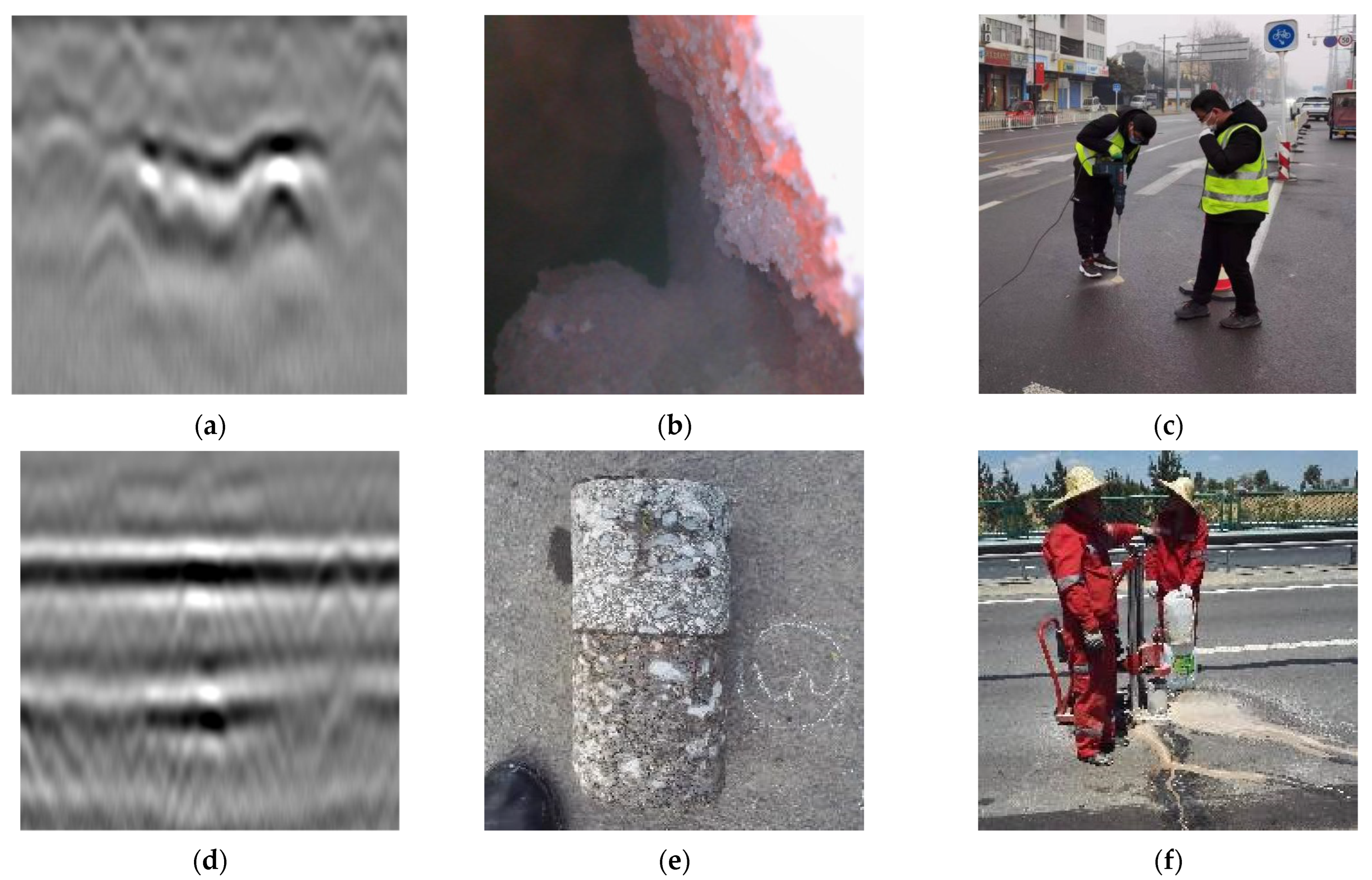
3.1. Field Data Collection

GPR data in this paper were all collected from field detection which was verified by experienced technicians and core drilling. Four urban roads and two highways in China were selected to ensure the diversity of data, and the total length is over 500 km, covering the southern, northern and central cities in China. Table 1 shows the detailed road structure. Four urban roads are in Zhengzhou, Kaifeng, and Xi’an, and two highways are in Anyang and Ningbo. The road structure is semi-rigid pavement that asphalt surface layers on semi-rigid base layers. The surface layer of the urban road consists of the upper layer and lower layer while highways consist of upper layer, middle layer and lower layer. Four-channel GPR system was used for the detection of the whole experiment road because it can be mounted on a vehicle with fast speed and high coverage area. Then, the hand-towed GPR device was used for detailed detection at the location of distresses. The two GPR systems mentioned above are ground-coupled data acquisition that shown in Figure 6. Figure 6a shows the Four-channel GPR system with one 200 MHz antenna, two 400 MHz antenna, and one 900 MHz antenna. Figure 6b shows the four-channel GPR system mounted on a vehicle. Figure 6c shows the hand-towed GPR device with a 400 MHz antenna. The collected GPR image and verified distress are shown in Figure 7. Figure 7a shows the GPR image of the cavity. Figure 7b shows that a cavity was verified by an industrial endoscope though a 2 cm diameter borehole. Figure 7c shows the electric hammer drill working at cavity distress. Figure 7d shows the GPR image of the crack. Figure 7e shows the crack verified by coring. Figure 7f shows the core drilling machine in crack distress. Most of the GPR data for training in this paper was collected by the hand-towing GPR device to ensure the quality of the data. The collected GPR data of cavity and crack distress is shown in Table 2. These samples are insufficient for training the deep learning model, so we could use the data augmentation to raise the number of training samples.

3.2. Data Augmentation

To further learn about the effectiveness of different data augmentation methods, we applied three strategies to establish the augmented GPR datasets by two times, four times, and eight times. Table 3 shows the statistics of augmented data for training. The data augmentation strategy was studied as follows: four training sessions were conducted at training datasets of 547, 1094, 2188, and 4376 images, and the same deep learning model was used with the only change in the data samples to study the training details on the model performance.

4. Result and Discussion

4.1. Evaluation Metrics

The training loss value of YOLOv7 consists of box_loss, cls_loss, obj_loss, and the total loss value is the sum of these three losses (as shown in Equation (5)).
Loss = box _ loss + cls _ loss + obj _ loss
In Equation (5), box_loss denotes the loss of object position, which measures how well the predicted bounding box locates an object. The IoU loss function was used to calculate the box_loss. The IoU is the ratio of the intersection and union between the predicted bounding box and the ground-truth box. The cls_loss denotes the loss of object category loss, which measures the probability that the region of interest exists an object. The obj_loss denotes the loss of whether it contains the object, which indicates how well the model can predict the object correctly [39].
To evaluate the performance of the data augmentation method in this paper, the following evaluation metrics were used, such as precision (P), recall (R), F1_score, and the mean average precision (mAP). Additionally, the evaluation metrics can be calculated as follows:
P = T P T P + F P
R = T P T P + F N
In Equations (6) and (7), T P is the number of true positives, which means that there is subsurface distress in the ground truth value, and so do prediction. F P is the number of false positives, it means that there is no subsurface distress in the ground truth value, but it is predicted that there is distress. F N is the number of false negatives, which is the opposite of F P . P denotes how well the model in classifying an object as positive, and R denotes the ability to detect the positive samples.
F 1 _ s c o r e = 2 P R P + R
A P = 0 1 P ( r ) d r
The values of F 1 _ s c o r e combines the result of P and R ranges from [0, 1], in which 1 denotes the best output of the model and 0 denotes the worst output of the model. A P is defined as the area under the P R curve, which measures the model’s accuracy for each class, and P ( r ) refers to the precision value for which the recall is r . m A P is the average of A P for all classes. m A P _ 0.5 is the mean average precision that the IoU threshold is 0.5. m A P _ 0.5 : 0.95 represents the average m A P at different IoU thresholds (from 0.5 to 0.95 in steps of 0.05).

4.2. Training Details

The YOLOv7 was trained and tested in the experiment. The detailed experimental environment configuration is shown in Table 4. As for the hyperparameters, the hyperparameters involved in this paper mainly include initialization parameters and training hyperparameters. To ensure the comparability of each case, we keep the parameter initialization consistent and use open-source pre-training parameters. In terms of training hyperparameters, this paper does not deliberately control the consistency but selects the hyperparameters that achieve the best results. However, it is found through experiments that the training hyperparameters for the best results for each case are the same, that is: the batch size is 16, the learning rate is 0.001, and the learning rate decays ten times after 100 epochs, and ten times again after 200 epochs.
To validate the effectiveness of data augmentation, the augmented GPR datasets by two times, four times, and eight times have been used for training the model. For every augmented dataset, a total of training epochs were set 300, input image size is 416*416. If the model’s performance was measured on the verification set at the end of the training process, it is also not representative [40]. So, eight evaluation metrics (box_loss, cls_loss, obj_loss, total loss, precision, recall, mAP_0.5, and mAP_0.5:0.95) were displayed as the training epochs increased during the training process.

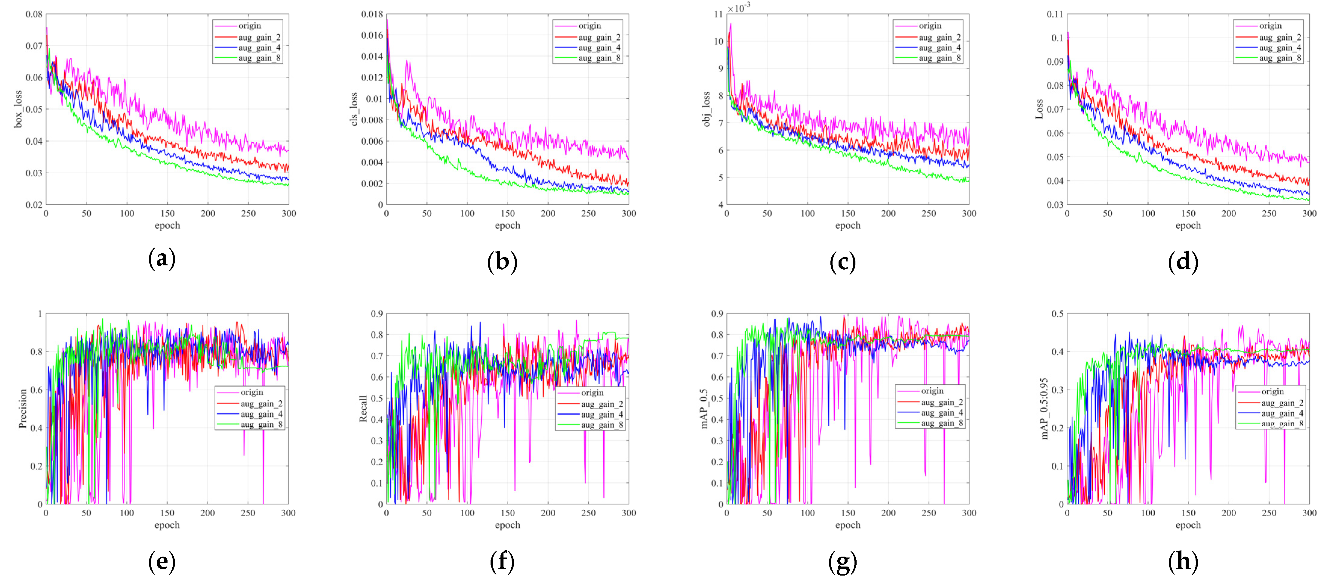
4.2.1. Image Brightness Transformation Based on Gain Compensation

Figure 8 shows the training details on the original and three augmented datasets using the gain compensation strategy. It can be seen that four types of loss functions on the verification set decrease when the training epochs grow. In addition, when the original datasets were augmented, the loss functions would decrease too, especially the cls_loss function trained on eight times datasets decreases rapidly compared to other datasets. At the same time, we used precision, recall, and mAP to evaluate the performance of different augmented datasets. The precision, recall, and mAP have been fluctuating during the model training on the original datasets. When the training datasets were augmented two times, four times, and eight times, these three metrics gradually become stable, proving that the augmented datasets can increase the robustness of the training model. The values of recall, mAP_0.5, and mAP_0.5:0.95 of the model were improved as the datasets increased, while the values of precision reached the maximum on the four times datasets. The gain compensation strategy considers the effect of gain on radar imaging, which can augment the datasets by simulating the EW propagation through different mediums. Therefore, this strategy can improve the value of recall very well but not always improve the value of precision when the datasets increase.

4.2.2. Image Resolution Transformations Based on Station Spacing

Figure 9 shows the training details on the original datasets and three augmented datasets by using the station spacing strategy. It can be seen that four types of loss functions on the verification set decrease when the training epochs grow. The model’s performance is not significantly improved when trained on the two times datasets. The values of cls_loss that trained on four times and eight times datasets decrease rapidly compared to the origin and two times datasets, and the final value is basically the same. At the same time, we use precision, recall, and mAP to evaluate the performance of different augmented datasets. The precision, recall, and mAP have fluctuated during the model training on the original datasets. When the training datasets were augmented two times, four times, and eight times, these three metrics gradually became stable, proving that the augmented datasets can increase the robustness of the training model. Although the model can converge fastest and is the most stable at the eight times datasets, the values of precision, recall, mAP_0.5, and mAP_0.5:0.95 reach the maximum when the model training on the four times augmented datasets. The station spacing strategy considers the effect of the setting parameters of the GPR device, which can augment the datasets by setting different station spacing when collecting the data.

4.2.3. Color Space Transformations Based on Radar Signal Mapping Rules

Figure 10 shows the training details on the original datasets and three augmented datasets by using the radar signal imaging strategy. It can be seen that four types of loss functions on the verification set decrease when the training epochs grow. The values of the four loss of model are not significantly decreased when training on the two times and four times datasets. However, when the model training on the eight times datasets, the values of four loss are decreased rapidly and the final value is the lowest. The precision, recall, and mAP have fluctuated when the model is trained on the original datasets. When the training datasets were augmented two times, four times, and eight times, these three metrics gradually become stable, proving that the augmented datasets can increase the robustness of the training model. Although the model can converge fastest and is the most stable at the eight times datasets, the values of precision, recall, mAP_0.5 and mAP_0.5:0.95 are the basically same when the model is trained on the four times augmented datasets. The radar signal imaging strategy takes into account the effect of the pixel value range when mapping the amplitude values into the image.

4.3. Comparative Study

4.3.1. Traditional Data Augmentation Methods

Then, we compare our data augmentation method with the traditional method in computer vision. The traditional method includes cropping, rotating, and flipping variations, which are realized by using the Albumentations [29]. Every traditional data augmentation strategy was used once to establish the GPR datasets and add the original datasets to obtain the four times augmented datasets. In this process, the crop size is randomly sampled from the range of [128, 256] pixels and resized to a 418 × 418 square image, the rotation angle is set to 15°, and the flipping variations are horizontal.

4.3.2. Results

We chose four times augmented datasets to train with the YOLOv7 model based on the training details that were studied above. All the augmented data are trained by the same deep learning model, and the performance of the model is compared in Table 5. The performance of the model training on the datasets augmented by strategy in this paper is better than the datasets augmented by using the traditional method. Compared to the traditional method, the results show that three data augmentation methods by incorporating domain knowledge can improve the precision rate by 10.45%, 8.99%, and 9.92%, respectively, and improve the recall rate by 9.80%, 1.96%, and 3.22%, improve the F1_score rate by 10.22%, 5.31%, and 6.40%, improve the mAP_0.5 rate by 3.71%, 1.79%, and 3.32%. For crack detection, in addition to the gain compensation strategy, the precision of the crack decreased when using the other augmented strategies. The morphology of the crack in the GPR image shows a typical hyperbolic shape, and the data augmentation strategies change the shape of the hyperbola to a certain extent, which leads to a drop in precision.

5. Conclusions

In this paper, we have proposed GPR data augmentation methods based on incorporating domain knowledge. The YOLOv7 model trains the augmented datasets to realize the automatic detection of the subsurface cavity and crack. These data augmentation methods can decrease loss function values when the training epochs grow. Additionally, the performance of the deep learning model gradually became stable when the original datasets were augmented two times, four times, and eight times, proving that the augmented datasets can increase the robustness of the training model. Compared with the traditional data augmentation method, the data augmentation method proposed in this paper incorporates domain knowledge of GPR. The gain compensation strategy considers the effect of gain on radar imaging, which can augment the datasets by simulating the EW propagation through different mediums. The station spacing strategy takes into account the impact of the setting parameters of the GPR device, which can augment the datasets by setting different station spacing when collecting the data. The radar signal imaging strategy takes into account the effect of the pixel value range when mapping the amplitude values into the image. In addition, our proposed method achieved higher precision, recall, F1_score, and mAP_0.5 compared with the traditional data augmentation method. However, we only chose a single data augmentation method and one deep learning model (YOLOv7) to study the impact of the model in this paper. Thus, a combination of different techniques and different deep learning models (such as Faster_CNN, SSD, Transformer, etc.), will be considered and compared for future work.

Author Contributions

Conceptualization, G.Y. and C.L.; methodology, G.Y.; C.L. and S.G.; software, Y.L.; validation, Y.L. and S.G.; formal analysis, G.Y.; investigation, G.Y.; data curation, G.Y. and S.G.; writing—original draft preparation, G.Y.; writing—review and editing, G.Y.; project administration, C.L.; funding acquisition, Y.D. and C.L. All authors have read and agreed to the published version of the manuscript.

Funding

This work is supported by the National key research and development program of China (2021YFB1600100), and the Scientific Research Project of the Shanghai Science and Technology Commission (21DZ1200601).

Institutional Review Board Statement

Not applicable.

Informed Consent Statement

Not applicable.

Data Availability Statement

The data used to support the findings of this study are available from the corresponding author upon request.

Conflicts of Interest

The authors declare no conflict of interest.

References

  1. Liu, C.; Wu, D.; Li, Y.; Du, Y. Large-scale pavement roughness measurements with vehicle crowdsourced data using semi-supervised learning. Transp. Res. Part C Emerg. Technol. 2021, 125, 103048. [Google Scholar] [CrossRef]
  2. Du, Y.; Weng, Z.; Li, F.; Ablat, G.; Wu, D.; Liu, C. A novel approach for pavement texture characterisation using 2D-wavelet decomposition. Int. J. Pavement Eng. 2022, 23, 1851–1866. [Google Scholar] [CrossRef]
  3. Liu, C.; Nie, T.; Du, Y.; Cao, J.; Wu, D.; Li, F. A Response-Type Road Anomaly Detection and Evaluation Method for Steady Driving of Automated Vehicles. IEEE T. Intell. Transp. 2022, 1–12. [Google Scholar] [CrossRef]
  4. Yue, G.; Du, Y.; Liu, C.; Guo, S.; Li, Y.; Gao, Q. Road subsurface distress recognition method using multiattribute feature fusion with ground penetratin gradar. Int. J. Pavement Eng. 2022, 1–13. [Google Scholar] [CrossRef]
  5. Peng, M.; Wang, D.; Liu, L.; Shi, Z.; Shen, J.; Ma, F. Recent Advances in the GPR Detection of Grouting Defects behind Shield Tunnel Segments. Remote Sens. 2021, 13, 4596. [Google Scholar] [CrossRef]
  6. Guo, S.; Xu, Z.; Li, X.; Zhu, P. Detection and Characterization of Cracks in Highway Pavement with the Amplitude Variation of GPR Diffracted Waves: Insights from Forward Modeling and Field Data. Remote Sens. 2022, 14, 976. [Google Scholar] [CrossRef]
  7. Benedetto, A.; Tosti, F.; Bianchini Ciampoli, L.; D Amico, F. An overview of ground-penetrating radar signal processing techniques for road inspections. Signal Process. 2017, 132, 201–209. [Google Scholar] [CrossRef]
  8. Lei, W.; Hou, F.; Xi, J.; Tan, Q.; Xu, M.; Jiang, X.; Liu, G.; Gu, Q. Automatic hyperbola detection and fitting in GPR B-scan image. Automat. Constr. 2019, 106, 102839. [Google Scholar] [CrossRef]
  9. Hwang, J.; Kim, D.; Li, X.; Min, D. Polarity Change Extraction of GPR Data for Under-road Cavity Detection: Application on Sudeoksa Testbed Data. J. Environ. Eng. Geoph. 2019, 24, 419–431. [Google Scholar] [CrossRef]
  10. Frigui, H.; Gader, P. Detection and Discrimination of Land Mines in Ground-Penetrating Radar Based on Edge Histogram Descriptors and a Possibilistic K-Nearest Neighbor Classifier. IEEE Trans. Fuzzy Syst. 2009, 17, 185–199. [Google Scholar] [CrossRef]
  11. Todkar, S.S.; Le Bastard, C.; Baltazart, V.; Ihamouten, A.; Dérobert, X. Performance assessment of SVM-based classification techniques for the detection of artificial debondings within pavement structures from stepped-frequency A-scan radar data. NDT E Int. 2019, 107, 102128. [Google Scholar] [CrossRef]
  12. Xu, J.; Zhang, J.; Sun, W. Recognition of the Typical Distress in Concrete Pavement Based on GPR and 1D-CNN. Remote Sens. 2021, 13, 2375. [Google Scholar] [CrossRef]
  13. Krizhevsky, A.; Sutskever, I.; Hinton, G.E. ImageNet Classification with Deep Convolutional Neural Networks. Commun. ACM 2017, 60, 84–90. [Google Scholar] [CrossRef] [Green Version]
  14. Gao, J.; Yuan, D.; Tong, Z.; Yang, J.; Yu, D. Autonomous pavement distress detection using ground penetrating radar and region-based deep learning. Measurement 2020, 164, 108077. [Google Scholar] [CrossRef]
  15. Hou, F.; Lei, W.; Li, S.; Xi, J.; Xu, M.; Luo, J. Improved Mask R-CNN with distance guided intersection over union for GPR signature detection and segmentation. Automat. Constr. 2021, 121, 103414. [Google Scholar] [CrossRef]
  16. Chen, S.; Wang, L.; Fang, Z.; Shi, Z.; Zhang, A. A Ground-penetrating Radar Object Detection Method Based on Deep Learning. In Proceedings of the 2021 IEEE 4th International Conference on Electronic Information and Communication Technology (ICEICT), Xi’an, China, 18–20 August 2021; pp. 110–113. [Google Scholar] [CrossRef]
  17. Li, X.; Liu, H.; Zhou, F.; Chen, Z.; Giannakis, I.; Slob, E. Deep learning-based nondestructive evaluation of reinforcement bars using ground penetrating radar and electromagnetic induction data. Comput. Aided Civ. Inf. 2021. [Google Scholar] [CrossRef]
  18. Liu, W.; Anguelov, D.; Erhan, D.; Szegedy, C.; Reed, S.; Fu, C.Y.; Berg, A.C. SSD: Single Shot Multi Box Detector. In Proceedings of European Conference on Computer Vision, Amsterdam, The Netherlands, 8–16 October 2016; Springer: Berlin, Germany, 2016; pp. 21–37. [Google Scholar] [CrossRef] [Green Version]
  19. Redmon, J.; Farhadi, A. YOLOv3: An Incremental Improvement. arXiv 2018, arXiv:1804.02767. [Google Scholar]
  20. Duan, K.; Bai, S.; Xie, L.; Qi, H.; Huang, Q.; Tian, Q. CenterNet: Keypoint Triplets for Object Detection. In Proceedings of the 2019 IEEE/CVF International Conference on Computer Vision (ICCV), Seoul, Korea, 27 October–2 November 2019; pp. 6568–6577. [Google Scholar]
  21. Lin, T.-Y.; Goyal, P.; Girshick, R.B.; He, K.; Dollar, P. Focal Loss for Dense Object Detection. IEEE Trans. Pattern Anal. Mach. Intell. 2020, 42, 318–327. [Google Scholar] [CrossRef] [Green Version]
  22. Wang, C.; Bochkovskiy, A.; Liao, H.M. YOLOv7: Trainable bag-of-freebies sets new state-of-the-art for real-time object detectors. arXiv 2022, arXiv:2207.02696. [Google Scholar]
  23. Li, Y.; Che, P.; Liu, C.; Wu, D.; Du, Y. Cross-scene pavement distress detection by a novel transfer learning framework. Comput. Aided Civ. Inf. 2021, 36, 1398–1415. [Google Scholar] [CrossRef]
  24. Bralich, J.; Reichman, D.; Collins, L.; Malof, J. Improving convolutional neural networks for buried target detection in ground penetrating radar using transfer learning via pretraining. In Detection and Sensing of Mines, Explosive Objects, and Obscured Targets XXII; International Society for Optics and Photonics: Anaheim, CA, USA, 2017; p. 101820X. [Google Scholar] [CrossRef]
  25. Ozkaya, U.; Ozturk, S.; Melgani, F.; Seyfi, L. Residual CNN plus Bi-LSTM model to analyze GPR B scan images. Automat. Constr. 2021, 123, 103525. [Google Scholar] [CrossRef]
  26. Qin, H.; Zhang, D.; Tang, Y.; Wang, Y. Automatic recognition of tunnel lining elements from GPR images using deep convolutional networks with data augmentation. Automat. Constr. 2021, 130, 103830. [Google Scholar] [CrossRef]
  27. Perez, L.; Wang, J. The Effectiveness of Data Augmentation in Image Classification using Deep Learning. arXiv 2017, arXiv:1712.04621. [Google Scholar]
  28. Liu, H.; Lin, C.; Cui, J.; Fan, L.; Xie, X.; Spencer, B.F. Detection and localization of rebar in concrete by deep learning using ground penetrating radar. Automat. Constr. 2020, 118, 103279. [Google Scholar] [CrossRef]
  29. Buslaev, A.; Iglovikov, V.I.; Khvedchenya, E.; Parinov, A.; Druzhinin, M.; Kalinin, A.A. Albumentations: Fast and Flexible Image Augmentations. Information 2020, 11, 125. [Google Scholar] [CrossRef] [Green Version]
  30. Zong, Z.; Chen, C.; Mi, X.; Sun, W.; Song, Y.; Li, J.; Dong, Z.; Huang, R.; Yang, B. A Deep Learning Approach for Urban Underground Objects Detection from Vehicle-Borne Ground Penetrating Radar Data in Real-Time. In Proceedings of the International Archives of the Photogrammetry, Remote Sensing and Spatial Information Sciences, Munich, Germany, 18–20 September 2019; Volume 42, pp. 293–299. [Google Scholar] [CrossRef] [Green Version]
  31. Sonoda, J.; Kimoto, T. Object Identification form GPR Images by Deep Learning. In Proceedings of the 2018 Asia-Pacific Microwave Conference (APMC), Kyoto, Japan, 6–9 November 2018; pp. 1298–1300. [Google Scholar] [CrossRef]
  32. Veal, C.; Dowdy, J.; Brockner, B.; Anderson, D.T.; Ball, J.E.; Scott, G. Generative adversarial networks for ground penetrating radar in hand held explosive hazard detection. In Detection and Sensing of Mines, Explosive Objects, and Obscured Targets XXIII; SPIE: Orlando, FL, USA, 2018; p. 106280T. [Google Scholar] [CrossRef]
  33. Li, J.; Madry, A.; Peebles, J.; Schmidt, L. On the Limitations of First-Order Approximation in GAN Dynamics. In Proceedings of the 35th International Conference on Machine Learning, Stockholm, Sweden, 10–15 July 2018; pp. 3005–3013. [Google Scholar]
  34. Chen, G.; Bai, X.; Wang, G.; Wang, L.; Luo, X.; Ji, M.; Feng, P.; Zhang, Y. Subsurface Voids Detection from Limited Ground Penetrating Radar Data Using Generative Adversarial Network and YOLOV5. In Proceedings of the 2021 IEEE International Geoscience and Remote Sensing Symposium IGARSS, Brussels, Belgium, 12 October 2021; pp. 8600–8603. [Google Scholar] [CrossRef]
  35. Bianchini Ciampoli, L.; Tosti, F.; Economou, N.; Benedetto, F. Signal Processing of GPR Data for Road Surveys. Geosciences 2019, 9, 96. [Google Scholar] [CrossRef]
  36. Li, Y.; Liu, C.; Yue, G.; Gao, Q.; Du, Y. Deep learning-based pavement subsurface distress detection via ground penetrating radar data. Automat. Constr. 2022, 142, 104516. [Google Scholar] [CrossRef]
  37. Verdonck, L.; Taelman, D.; Vermeulen, F.; Docter, R. The Impact of Spatial Sampling and Migration on the Interpretation of Complex Archaeological Ground-penetrating Radar Data. Archaeol. Prospect. 2015, 22, 91–103. [Google Scholar] [CrossRef]
  38. Zhang, X.; Zeng, H.; Guo, S.; Zhang, L. Efficient Long Range Attention Network for Image Super resolution. arXiv 2022, arXiv:2203.06697. [Google Scholar]
  39. Kasper-Eulaers, M.; Hahn, N.; Berger, S.; Sebulonsen, T.; Myrland, Ø.; Kummervold, P.E. Short Communication: Detecting Heavy Goods Vehicles in Rest Areas in Winter Conditions Using YOLOv5. Algorithms 2021, 14, 114. [Google Scholar] [CrossRef]
  40. Reichman, D.; Collins, L.M.; Malof, J.M. Some good practices for applying convolutional neural networks to buried threat detection in Ground Penetrating Radar. In Proceedings of the 2017 9th International Workshop on Advanced Ground Penetrating Radar (IWAGPR), Edinburgh, UK, 28–30 June 2017; pp. 1–5. [Google Scholar] [CrossRef]
Figure 1. GPR data augmentation methods by incorporating domain knowledge: image brightness transformation based on gain compensation, image resolution transformations based on station spacing, and color space transformations based on radar signal mapping rules.
Applsci 12 10896 g001
Figure 2. (a) The original GPR image; (bh) are the GPR images that were generated with 0.2, 0.4, 0.6, 0.8, 1.2, 1.4, and 1.6 gain coefficients.
Applsci 12 10896 g002
Figure 3. (a) Multiple A-scan traces along the survey line; (b) the GPR image in grayscale.
Applsci 12 10896 g003
Figure 4. (a) The original GPR image; (bh) are the interval 1, 2, 3, 4, 5, 6, 7 traces are selected to extract one single signal, respectively.
Applsci 12 10896 g004
Figure 5. (a) The original GPR image at gray mapping rules; (bh) are the GPR image at afmhot, bwr, cool, jet, ocean, rainbow, and RdGy mapping rules, respectively.
Applsci 12 10896 g005
Figure 6. (a) The four-channel GPR system (b) GPR system was mounted on a vehicle; (c) the hand-towed GPR device.
Applsci 12 10896 g006
Figure 7. (a) The GPR image of cavity; (b) cavity was verified by an industrial endoscope; (c) field picture at cavity distress location; (d) the GPR image of crack; (e) crack was verified by coring; (f) field picture at crack distress location.
Applsci 12 10896 g007
Figure 8. The training details of gain compensation augmentation strategy: (a) box_loss; (b) cls_loss; (c) obj_loss; (d) total of three loss; (e) precision; (f) recall; (g) mAP_0.5; (h) mAP_0.5:0.95.
Applsci 12 10896 g008
Figure 9. The training details of station spacing augmentation strategy: (a) box_loss; (b) cls_loss; (c) obj_loss; (d) total of three loss; (e) precision; (f) recall; (g) mAP_0.5; (h) mAP_0.5:0.95.
Applsci 12 10896 g009
Figure 10. The training details of radar signal imaging augmentation strategy: (a) box_loss; (b) cls_loss; (c) obj_loss; (d) total of three loss; (e) precision; (f) recall; (g) mAP_0.5; (h) mAP_0.5:0.95.
Applsci 12 10896 g010aApplsci 12 10896 g010b
Table 1. Road structures.
RoadsUrban RoadHighway
LocationZhengzhou
Henan
Kaifeng
Henan
Xi’an
Shaanxi
Huainan
Anhui
Anyang
Henan
Ningbo
Zhejiang
SurfacesUpper layers4 cm AC-16C4 cm AC-13C4 cm AC-13C4 cm AC-13C4 cm AC-13C4 cm SMA-13
Middle layers////6 cm AC-16C6 cm AC-16C
Lower layers6 cm AC-20C6 cm AC-16C6 cm AC-16C6 cm AC-16C9 cm AC-20C10 cm ATB-25
BasesUpper bases18 cm Cement stabilized gavels18 cm Cement stabilized gavels20 cm Cement stabilized gavels8 cm Cement stabilized gavels18 cm Cement stabilized gavels20 cm Cement stabilized gavels
Lower Bases18 cm cement stabilized gavels18 cm cement stabilized gavels20 cm cement stabilized gavels20 cm Granular18 cm cement stabilized gavels20 cm cement stabilized gavels
Table 2. The statistics of collected field data.
Training SetValidation SetTesting Set
The number of cavities3124848
The number of cracks2716363
The number of images547108108
Table 3. The statistics of augmented data for training.
AugmentationsGain CompensationStation SpacingRadar Signal Imaging
2 Times4 Times8 Times2 Times4 Times8 Times2 Times4 Times8 Times
The number of cavities624124824966241248249662412482496
The number of cracks542108421685421084216854210842168
The number of images109421884376109421884376109421884376
Table 4. The configuration of the environment.
ParametersConfiguration
System environmentLinux
GPUNVIDIA GTX 1080Ti
GPU accelerationCUDA 10.1
Training frameworkPytorch 1.12.1
LanguagePython 3.9.12
Table 5. The performance of model comparison using different augmented data for training.
AugmentationsOriginalGain CompensationStation SpacingRadar Signal Mapping RulesTraditional Method
CavityCrackAllCavityCrackAllCavityCrackAllCavityCrackAllCavityCrackAll
precision0.5840.9120.7480.7470.9220.8350.7690.8790.8240.7630.8990.8310.6630.8490.756
recall0.7910.6190.7050.8540.7130.7840.8330.6230.7280.8210.6520.7370.7780.6490.714
F1_score0.6720.7370.7260.7970.8040.8090.8000.7290.7730.7910.7560.7810.7160.7360.734
mAP_0.50.7310.8200.7760.7960.8270.8110.8110.7810.7960.7970.8190.8080.8150.7490.782
Publisher’s Note: MDPI stays neutral with regard to jurisdictional claims in published maps and institutional affiliations.

