GNSS-Based Dam Monitoring: The Application of a Statistical Approach for Time Series Analysis to a Case Study

Abstract

Dams are one of the most important engineering works of the current human society, and it is crucial to monitor and obtain analytical data to log their conditions, predict their behavior and, eventually, receive early warnings for planning interventions and maintenance activities. In this context, GNSS-based point displacement monitoring is nowadays a consolidated technique that is able to provide daily millimeter level accuracy, even with less sophisticated and less expensive single-frequency equipment. If properly designed, daily records of such monitoring systems produce time series that, when long enough, allow for an accurate reconstruction of the geometrical deformation of the structure, thus guiding semi-automatic early warning systems. This paper focuses on the procedure for the GNSS time series processing with a statistical approach. In particular, real-world times series collected from a dam monitoring test case are processed as an example of data filtering. A remove–restore technique based on a collocation approach is applied here. Basically, it consists of an initial deterministic modeling by polynomials and periodical components through least squares adjustment and Fourier transform, respectively, followed by a stochastic modeling based on empirical covariance estimation and a collocation approach. Filtered time series are interpreted by autoregressive models based on environmental factors such as air or water temperature and reservoir water level. Spatial analysis is finally performed by computing correlations between displacements of the monitored points, as well as by visualizing the overall structure deformation in time. Results positively validate the proposed data processing workflow, providing useful hints for the implementation of automatic early warning systems in the framework of structural monitoring based on continuous displacement measurements.

1. Introduction

Monitoring civil infrastructures plays a key role in ensuring their safety conditions and maintaining their operational functions during the whole lifecycle. Infrastructural systems are subject to aging and are under continuous operational stress, and sometimes additional overstress due to exceptional events may occur. For this reason, without adequate control and monitoring systems, they can represent serious risks of losses for the society from several perspectives: economic, environmental and even for the health and safety of people. In this context, Italian infrastructures are considered at high risk, with Italy being particularly sensitive to natural hazards [1,2]. In the period 1944–2017, landslides, floods and earthquakes caused about 10,000 victims and led to estimated economic losses of about 290 billion euros [3].

Among all civil infrastructures, dams are one of the most important engineering structures of the current human society. They supply water for domestic and industrial use and irrigation purposes and are also involved in hydroelectric power generation and river navigation. Thus, it is crucial to monitor and gather analytical data to log their conditions, predict their behavior and, eventually, receive early warnings for planning interventions and maintenance activities. The failure of dams, although rare, can be catastrophic and may cause immense damage and loss of life [4]. The most extreme example is the sequential failure in 1975 of the Banqiao Reservoir Dam and more than 60 others in Henan Province, China. Dramatically, the official number of victims caused by this event was 26,000 [5]. Dam health monitoring plays an important role in securing their structural integrity and maintaining their longevity. It calls for the use of multiple sensors for monitoring a wide variety of quantities such as body deformation, point displacements, temperature, uplift and pore pressures, seepage and drainage rates, and piezometric level, just to cite the most significant ones [6]. Regarding the measurement of displacements and deformation, i.e., the geometric variation of the dam and its surroundings, the typical approach consists of monitoring a set of Control Points (CPs) established properly in key positions (e.g., the dam crest, the downstream banks, the lateral abutments) to retrieve the general behavior of the whole structure. Several techniques have been developed and applied by exploiting technological advancements that brought innovation and enhancements in terms of acquisition rate, spatial coverage, accuracy, and automation.

Since the beginning of the 20th century, the static monitoring of dams was mainly based on geodetic control networks by applying classical techniques such as precision triangulation and geometric leveling [7,8]. Such measurements of absolute and relative displacements of the structure and of the nearby areas were often complemented or integrated with other measurement methods based on geotechnics and structural sensors, e.g., direct and inverted pendulums, rock meters, tiltmeters, strain meters and clinometers [9,10,11]. The main drawbacks of such monitoring systems were essentially the necessity of favorable atmospheric conditions, specialized personnel and expert surveyors, as well as the long duration of both the measurements and processing procedures [12]. Starting from the 1960s, total electronic motorized stations, digital levels and, in general, the introduction of automatic data reading, acquisition, recording, and telemetric transmission allowed for continuous monitoring, thus providing denser long-term data series and subsequently enhancing the capability of analyzing deformation patterns [13,14].

As happened with remote sensing techniques [15,16,17,18], the application of methods based on Global Navigation Satellite Systems (GNSS) is now consolidated, where GNSS networks of points are measured with reference to proximal CORS (Continuously Operating Reference Station) or other stations established on purpose in nearby stable areas [19,20,21,22]. More recently, automatic systems based on GNSS positioning have been developed to be integrated into early-warning systems for dam safety management [23,24]. Furthermore, recent research proved that low-cost and mass-market GNSS equipment can also be properly used for structural monitoring purposes, and adequate accuracies and system integrity can be reached without geodetic level instrumentation [25,26,27,28], making the GNSS approach even more attractive and widespread. In fact, by reducing the overall cost of the GNSS monitoring systems, more CPs can be instrumented, and a more comprehensive and broad reconstruction of the dam displacement/deformation over time and space is attainable.

In the framework of GNSS dam monitoring, the typical setup consists of a (or more) reference station installed on a stable platform located some hundred to thousands of meters apart from the dam body, several monitoring stations on the dam crest, and in the case of earth embankments, on the downstream shell. Relative positioning is performed between the reference (considered fixed) and the monitoring points, and on the basis of 24 h continuous measurements, daily positioning solutions are provided [29,30,31]. The estimated positions are commonly framed in a previously established local reference frame with one of the horizontal axes parallel to the dam crest and an upward vertical axis. Three-dimensional CP displacements are typically considered independent of each other, and the corresponding temporal series represent the time-dependent position variations along the most meaningful directions, i.e., the dam crest, the reservoir up/downstream, and the altitude. Such temporal series suffer from measurement noise, and they are generally smoothed, filtering out the high-frequency variations by means of interpolation techniques [32]. The resulting 3D time series describes the dam displacement in correspondence with the monitored points. It is known that environmental factors and operation activities influence the displacements, and therefore, they should be modeled in order to analyze the residual data looking for unexpected trends or behaviors. Air/water temperature and reservoir water level are the main factors to be taken into account for computing the so-called HTT (Hydrostatic Temperature Time) model of displacements [33,34,35,36].

In this paper, a statistical approach for dam monitoring based on the use of GNSS techniques is described and detailed, taking as reference the experience of a real case of an embankment dam monitored with such a methodology. Despite the fact that results will be presented and discussed with reference to a real case, the goal of the manuscript is more associated with the accurate description of the methodological approach of these analyses, from the preliminary processing to the final interpretation, so as to set up a general and effective procedure for structural monitoring.

2. Materials and Methods

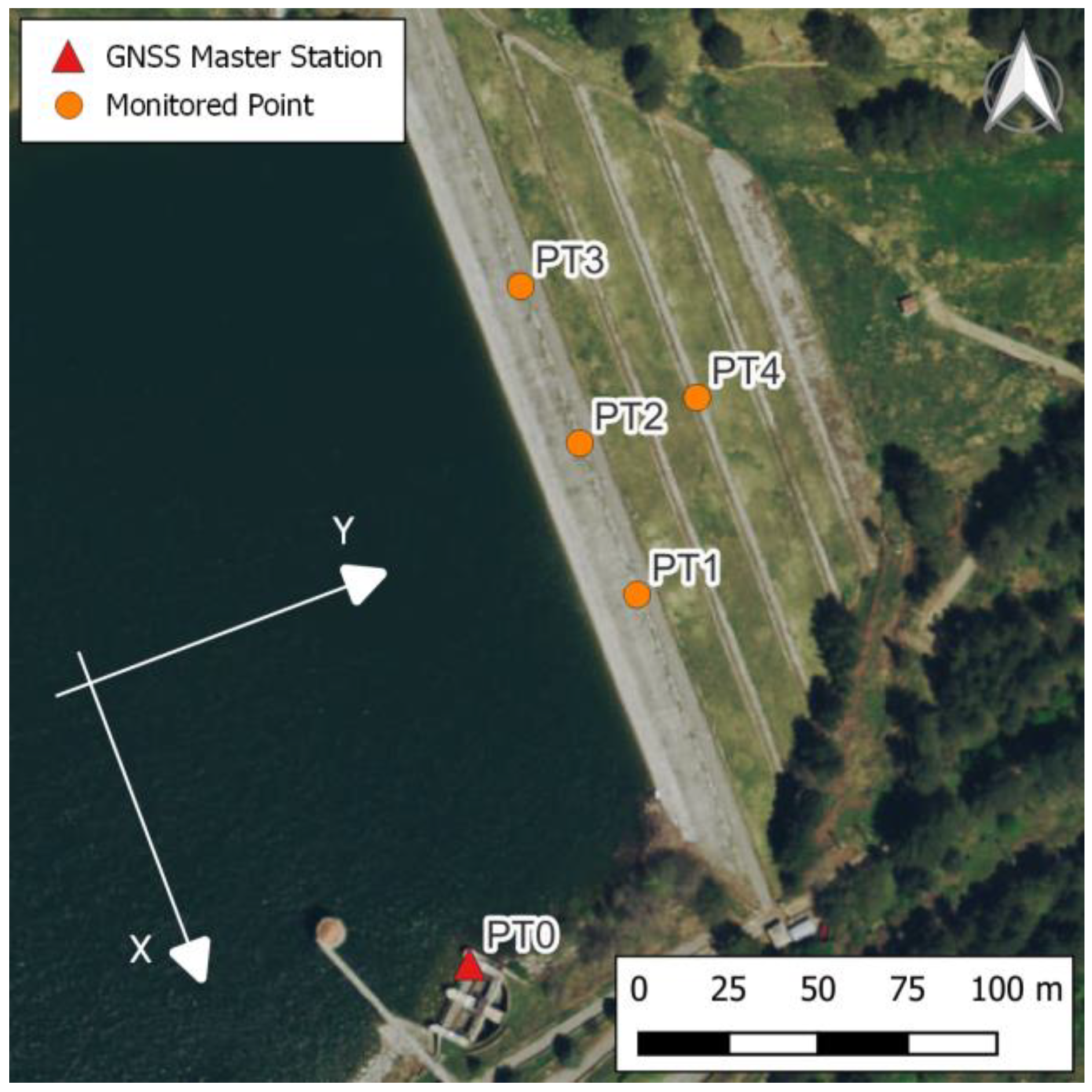
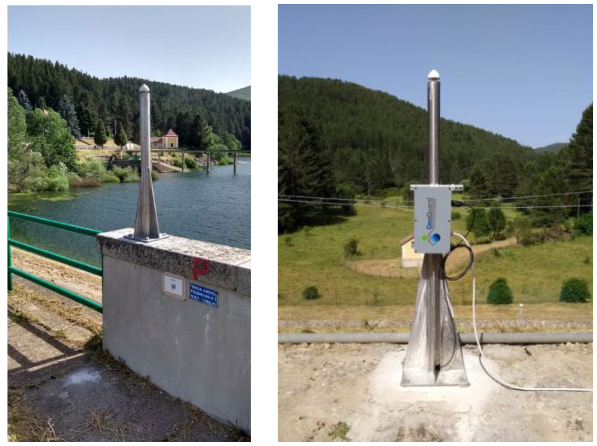
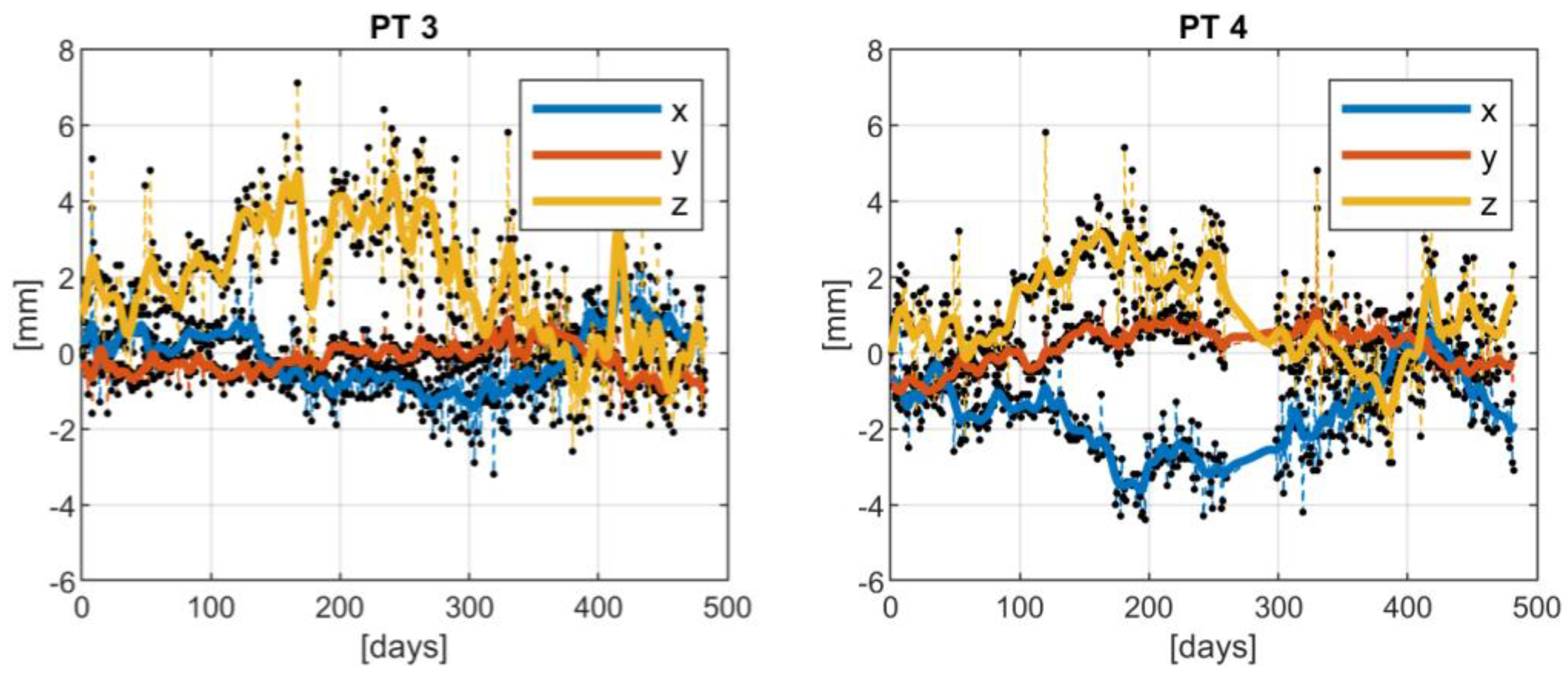
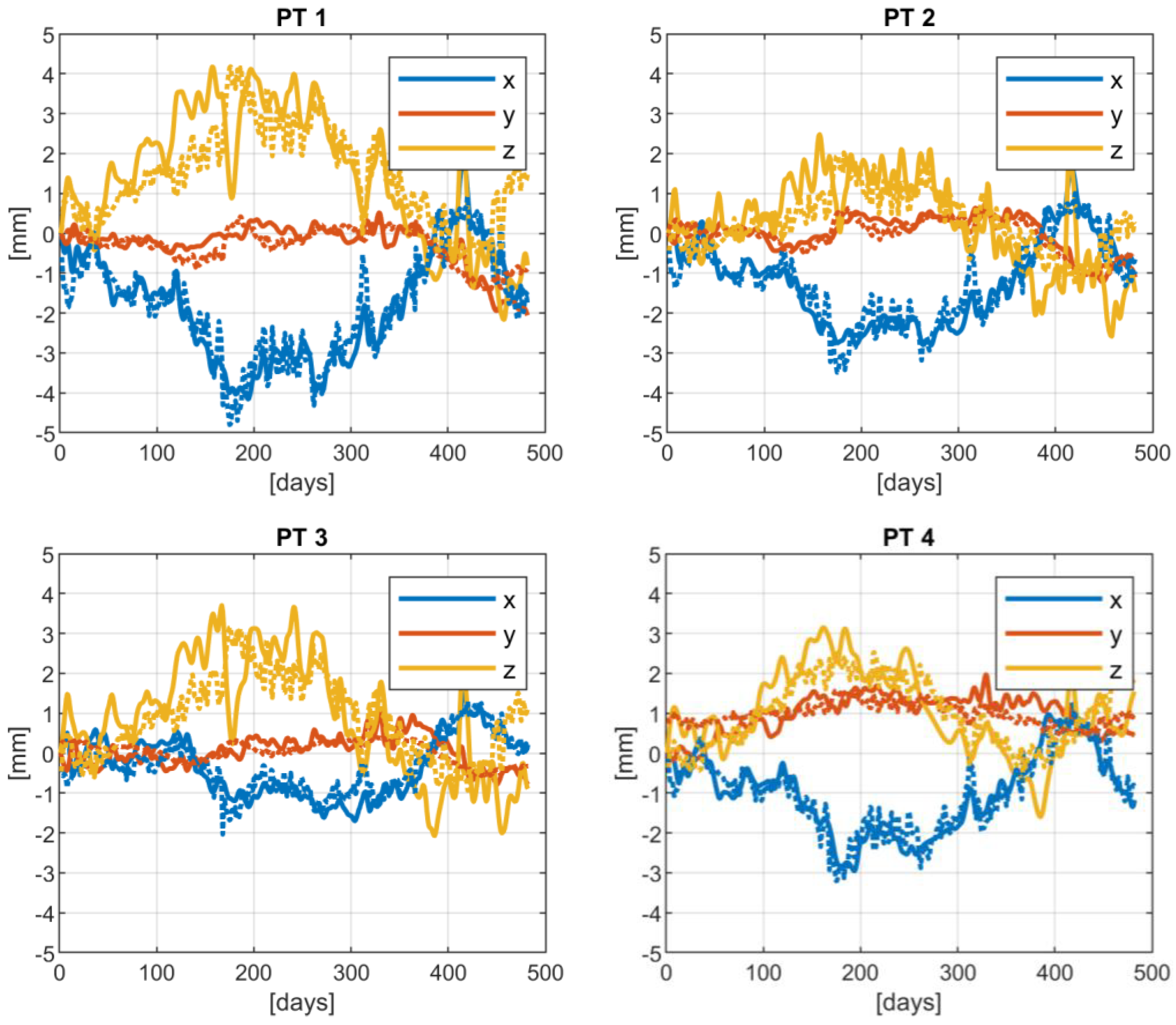
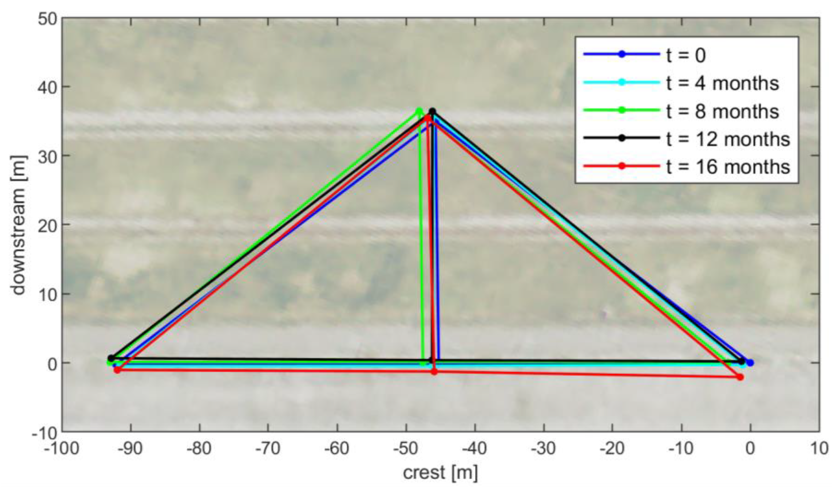
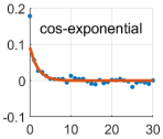
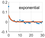
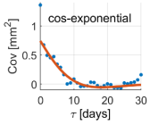
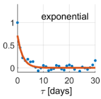
This section presents the real case of dam monitoring based on GNSS techniques and is taken as a reference to exemplify the methodological approach for the analysis and interpretation of the displacement time series logged by the GNSS monitoring system. Two subsections are reported. The first one focuses on the description of the monitored structure, its characteristics and the installed GNSS monitoring equipment. For security and privacy reasons, site and structure will be described in a general way, and any information that could potentially lead to identifying the location and/or the responsible personnel/organization/company of the dam will be omitted. The second subsection deals with the processing required to filter the raw time series for the subsequent displacement interpretation, with particular reference to a possible practical implementation in the framework of an early warning system.

2.1. GNSS Equipment, Installation and Raw Data Processing

Five single frequency u-blox NEO-M8T GNSS [37] receivers coupled with Tallysman TW3740 antennas were installed and distributed, as shown in Figure 1. With such receivers, millimetric accuracies have been proved to be achievable [25], in line with the requirements for dam monitoring. One (PT0) was located close, but outside the dam body and used as a reference point, three (PT1–3) were installed on the dam crest and one (PT4) on the downstream shell. PT0 was powered by a battery tied to a solar panel, while PT1–4 were connected to the electric network. Antennas mounted on the dam crest were connected to their receivers through coaxial cables with a maximum length of 50 m to reach the unique unit gathering all the receivers. In addition, PT0 was controlled by relative positioning with respect to the closest available CORS belonging to a national reference network.

For the installation of PT stations, steel pillars supporting the antennas were monumented on granite blocks integrated with the crest’s concrete walls or concrete plinths realized for the purpose. With such monumentations, the stability of the installed antennas was ensured, as well as sky visibility in the case of persistent snowfall (see Figure 2).

Daily position solutions were computed for each of the four PT1–4 stations through double-difference relative positioning with respect to the reference station PT0. Bernese 5.2 software was used to process the 5 s sampling observed sessions, and phase ambiguity resolution was performed by applying the Sigma method [38]. Since the baseline lengths are in the order of a few tens of meters and there is almost no height difference amongst the points, atmospheric effects such as tropospheric and ionospheric delays can be neglected by using the double difference approach [25]. The reference PT0 coordinates were previously determined on the basis of a static positioning session (one week long) performed by assuming the closest CORS as the reference station. ETRF2000-RDN [39] PT station coordinates were determined, but for the purpose of dam monitoring, a local reference system was defined. This local reference system was centered at PT0 with X-Y axes referring to the horizontal coordinates rotated to be aligned with the longitudinal and transversal directions of the dam. Time series of the 3D coordinates of the PT monitoring stations were computed and made suitable for further processing and analyses aiming at determining the detectable time-dependent displacements of the dam. The analyzed time series refer to the period Jul/2019–Nov/2020.

2.2. Displacement Time Series Analysis

The time series of the daily estimated displacements of each point along the three local XYZ axes needed to be filtered to properly manage the observation noise [40,41], fill possible gaps, and allow for a straightforward modeling and interpretation of the displacements. The filtering was performed by applying the collocation approach [42,43], thus modeling the signal in time as a stationary random process. A requirement for such an approach is that the signal to be treated is zero-mean, which is not guaranteed in the case of time series regarding point displacements. To fulfill this requirement, a remove–compute–restore scheme was adopted, where the first step consists of removing a deterministic trend from the observed data by modeling it as the sum of a polynomial and a periodical component. After this stage, the observed residual displacements were filtered by collocation, and finally, the deterministic trend was added back to the filtered time series to estimate the displacement.

Given the proposed scheme, we wrote the observation equation as:

$$d_o^{\left(j,k\right)}\left(t\right)=p^{\left(j,k\right)}\left(t\right)+q^{\left(j,k\right)}\left(t\right)+y^{\left(j,k\right)}\left(t\right)+\nu \left(t\right)$$

(1)

where, considering a point $j$ and a coordinate $k$, $p^{\left(j,k\right)}\left(t\right)$ and $q^{\left(j,k\right)}\left(t\right)$ are the polynomial and periodic deterministic trends, respectively, $y^{\left(j,k\right)}\left(t\right)$ the residual displacement to be stochastically modeled, and $\nu \left(t\right)$ the observation noise. Note that each $\left(j, k\right)$ combination was independently processed. Therefore, for the sake of simplicity, the $\left(j, k\right)$ indexes are omitted in the notation of the following equations.

The estimation of the polynomial trend was performed by least squares adjustment [44], expressing the polynomial as:

$$p\left(t\right)={\displaystyle \sum }_{i=0}^N{a}_i{t}^i$$

(2)

where $a_i$ are the coefficients to be estimated, and $N$ is the degree of the polynomial. The least squares adjustment was solved disregarding possible periodical components and residual displacements. To avoid an over parametrization of the interpolating function, the optimal polynomial degree $N$ needed to be calibrated. To this aim, a first estimate of the set of $a_i$ coefficients was performed with $N=\overline{N}$, where $\overline{N}$ is the maximum allowable degree. Then, a statistical test (t-test) to check whether the estimated value of the $N$-degree coefficient $a_N$ was significantly different from zero was applied. If the test hypothesis was accepted, the current $N$ degree of the polynomial was chosen as optimal; otherwise, the least squares adjustment was performed again after reducing the current degree $N$ by 1. This procedure was iterated until the null hypothesis on the $N$-degree coefficient was rejected.

As for the periodical component of the signal $q\left(t\right)$, it was determined by means of a Fourier analysis of the polynomial-reduced displacements $u\left(t\right)$, namely:

$$U\left(f\right)=\mathcal{F}\left(u\left(t\right)\right)=\mathcal{F}\left(d_o\left(t\right)-\widehat{p}\left(t\right)\right)$$

(3)

where $\mathcal{F}\left(\cdot \right)$ is the Fourier transform operator, $f$ is the frequency, and $\widehat{p}\left(t\right)$ is the previously estimated polynomial deterministic trend. Note that possible data gaps were filled by using the previously estimated polynomial trend to make the discrete Fourier transform applicable. These interpolated values were only used for the purpose of Fourier analysis. Given the transformed residuals $U\left(f\right)$, the empirical Amplitude Spectral Density (ASD) of $u\left(t\right)$ was computed as:

$$A_u\left(f\right)=\left|U\left(f\right)\right|$$

(4)

From Equation (4), a smoothed model ${\stackrel{-}{A}}_u$ of the ASD was determined by applying a moving median filter. The ratio between the empirical and filtered ASDs

$$r\left(f\right)=\frac{A_u\left(f\right)}{{\overline{A}}_u\left(f\right)}$$

(5)

was then used to identify the main frequencies carrying a periodical contribution in the signal. This periodical effect was decomposed in two parts, one related to low frequencies, i.e., in the range $\left|f\right|<{\overline{f}}_L$, and one related to high frequencies, i.e., in the range $\left|f\right|>{\overline{f}}_H$. Note that, according to the proposed model, the condition ${\overline{f}}_H\ge {\overline{f}}_L$ must always be satisfied. The choice of introducing two thresholds allows for flexibility in the data analysis, making it possible to adapt the analysis to the physical behavior of the considered phenomenon or structure, e.g., by excluding middle frequencies, i.e., ${\overline{f}}_H>\left|f\right|>{\overline{f}}_L$, from the analysis. Given the ratio $r\left(f\right)$ of Equation (5), a threshold $\overline{r}>1$ can be defined to identify the frequencies of the dominating periodical contributions, i.e., the frequencies satisfying the condition $r\left(f\right)>\overline{r}$. The periodical trends were then computed by an inverse Fourier transform of the coefficients $U\left(f\right)$ corresponding to the identified frequencies that are also included in the chosen frequency ranges (low or high frequencies). This translates into the following estimation equations:

$${\widehat{q}}_L\left(t\right)={\mathcal{F}}^{-1}\left(U\left(f\right)\left(1-\frac{1}{r\left(f\right)}\right){\chi }_L\left(f\right)\right)$$

(6)

$${\widehat{q}}_H\left(t\right)={\mathcal{F}}^{-1}\left(U\left(f\right)\left(1-\frac{1}{r\left(f\right)}\right){\chi }_H\left(f\right)\right)$$

(7)

where the characteristic functions ${\chi }_L\left(f\right)$ and ${\chi }_H\left(f\right)$ are defined as:

$${\chi }_L\left(f\right)=\left\{\begin{array}{c}1 \left|f\right|< {\overline{f}}_L\wedge r\left(f\right)>\overline{r}\\ 0 \mathrm{o}\mathrm{t}\mathrm{h}\mathrm{e}\mathrm{r}\mathrm{w}\mathrm{i}\mathrm{s}\mathrm{e} \end{array}\right.$$

(8)

$${\chi }_H\left(f\right)=\left\{\begin{array}{c}1 \left|f\right|>{\overline{f}}_H\wedge r\left(f\right)>\overline{r}\\ 0 \mathrm{o}\mathrm{t}\mathrm{h}\mathrm{e}\mathrm{r}\mathrm{w}\mathrm{i}\mathrm{s}\mathrm{e} \end{array}\right.$$

(9)

Note that the introduction of the scale factor $\left(1-\frac{1}{r\left(f\right)}\right)$ before the inverse Fourier transform in Equations (6) and (7) was required to empirically distinguish the periodical from the stochastic component under the assumption that the ASD of the stochastic component was equal to the moving-median ASD.

In summary, the overall periodical effect was determined as:

$$\widehat{q}\left(t\right)={\widehat{q}}_L\left(t\right)+{\widehat{q}}_H\left(t\right)$$

(10)

In the following, the detected low and high-frequency components were treated with a different approach. In particular, the former was assumed to be related to the physical phenomenon, while the latter to the noise. Therefore, they were both removed from the observations, but only the low-frequency periodical component ${\widehat{q}}_L\left(t\right)$ was subsequently restored after the collocation step.

Once polynomial and periodical deterministic trends were computed, they were used to reduce the signal and isolate the observations of the stochastic component $y\left(t\right)$ from the overall displacement observations $d_o\left(t\right)$. Therefore, the observation equation becomes:

$$y_o\left(t\right)=d_o\left(t\right)-\widehat{p}\left(t\right)-{\widehat{q}}_L\left(t\right)-{\widehat{q}}_H\left(t\right)+\nu \left(t\right)=\tilde{y}\left(t\right)+\nu \left(t\right)=y\left(t\right)+\eta \left(t\right)$$

(11)

where $\eta \left(t\right)$ includes both the measurement noise $\nu \left(t\right)$ and the estimation error of the polynomial and periodical deterministic components. For the sake of simplicity, the possible correlations between $y\left(t\right)$ and $\eta \left(t\right)$ were neglected and $\eta \left(t\right)$ was assumed to be white.

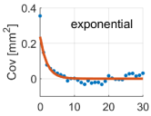
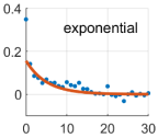
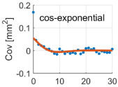
Given the observations reduced as in Equation (11), the empirical covariance function of the signal was determined as:

$$C^e\left(\tau \right)=\frac{1}{N_{\tau }}{\displaystyle \sum }_{}^i{y}_o\left(t_i\right)y_o\left(t_i-\tau \right)$$

(12)

where the summation extends $\forall t \in T: \left(t-\tau \right) \in T$, with $T$ being the overall set of observation epochs, and $N_{\tau }$ is the number of couples for a given $\tau$. The empirical covariance function was used to determine an analytical covariance model $\widehat{C}\left(\tau \right)$, along with the determination of ${\sigma }_{\eta }^2$. In particular, $\widehat{C}\left(\tau \right)$ was determined by a best fit procedure on $C^e\left(\tau \right)$ for $\left|\tau \right|>0$ since at $\tau =0$, the empirical covariance combines signal and noise, according to the assumption of a white $\eta \left(t\right)$. Once the model $\widehat{C}\left(\tau \right)$ was defined, the variance of the noise was computed as:

$${\widehat{\sigma }}_{\eta }^2=C^e\left(0\right)-\widehat{C}\left(0\right)$$

(13)

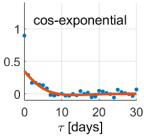
The best covariance model was chosen among several candidate models as the one with the lowest residuals between the empirical and analytical covariances. Then, the collocation estimate of the filtered signal was computed as:

$$\widehat{y}\left(\mathit{t}\right)={\mathrm{C}}_{yy}\left(\mathit{t},{\mathit{t}}_o\right){\left[{\mathrm{C}}_{yy}\left({\mathit{t}}_o,{\mathit{t}}_o\right)+{\sigma }_{\eta }^{2}I\right]}^{-1}{y}_o\left({\mathit{t}}_o\right)$$

(14)

where the $\mathit{t}$ and ${\mathit{t}}_o$ are the vectors containing the estimation and observation epochs, respectively, and the notation ${\mathrm{C}}_{yy}\left({\mathit{t}}_o,{\mathit{t}}_o\right)$ represents the covariance matrix computed by evaluating the model covariance $\widehat{C}\left(\tau \right)$ for all the possible time lags $\tau$ coming from the possible combinations of the elements of the vectors ${\mathit{t}}_o$.

Finally, from the output of Equation (14), the modeled displacement at the estimation epochs $\mathit{t}$ was computed by restoring the polynomial and periodical components as

$$\widehat{d}\left(\mathit{t}\right)=\widehat{y}\left(\mathit{t}\right)+\widehat{p}\left(\mathit{t}\right)+{\widehat{q}}_L\left(t\right)$$

(15)

3. Results

The observed GNSS displacements were filtered by means of the procedure previously explained in Section 2.2. As already stated, we independently processed the displacement time series of each coordinate (x, y, and z) and point (PT1, 2, 3 and 4), leading to twelve different analyses. In the following, the way in which the filtering algorithm has been applied is described, also explaining the choice and calibration of the different algorithm parameters.

As for the polynomial interpolation (Equation (2)), a maximum degree $\overline{N}=3$ was considered. In other words, only linear, quadratic, and cubic functions were considered as possible trends. The iterative approach for determining the optimal degree $N$ of the interpolating functions was performed by considering a 5% significance level for the t-test.

Table 1. Degree of the polynomial trends used to reduce the observed displacements.

Coordinate	PT1	PT2	PT3	PT4
x	cubic	cubic	cubic	cubic
y	cubic	cubic	cubic	quadratic
z	cubic	cubic	cubic	cubic

shows the resulting degree for each coordinate of each point.

Regarding the periodical deterministic component, the first step was to choose the threshold frequencies ${\overline{f}}_L$ and ${\overline{f}}_H$, in order to define the low and high frequency ranges. These two ranges were defined by considering periods longer than 25 days (for the low-frequency range) and smaller than 3 days (for the high-frequency range). To identify the periodical trend, a threshold $\overline{r}=2$ was chosen (see Equation (5)) and therefore this trend was reconstructed from the Fourier coefficients having a power that is at least double the one of the background signal. An example of this analysis is reported in Figure 3, considering the point PT1, showing the empirical and moving-median ASDs and flagging with stars the identified periodical frequencies that were modeled and removed from the signal by means of Equations (6) and (7).

Note that, to apply the discrete Fourier transform (DFT), it was required to work with regularly sampled data. In general, this requirement is satisfied thanks to GNSS daily solutions. However, there are few gaps in the data, e.g., related to temporary anomalies of the receivers or errors in the data transfer. In general, missing data were less than 2% of the whole period, apart from time series of the point PT4, in which there was about 10% missing data due to a receiver fault in March 2020. To allow the usage of DFT, these data gaps were filled with values computed by the polynomial deterministic trends estimated at the previous step, without a significant impact on the periodical component analysis.

Once the observed displacements were reduced for polynomial and periodical deterministic trends, we applied the stochastic analysis based on the collocation approach. To this aim, the first step was to compute the empirical covariance function and to fit it with a model. The candidate models proposed in this analysis were: exponential, cosine-exponential, Gaussian, cosine-Gaussian and power-Gaussian, shown in Equations (6)–(20), respectively.

$$C\left(\tau \right)=b_1\exp \left(-b_2\tau \right)$$

(16)

$$C\left(\tau \right)=b_1\exp \left(-b_2\tau \right)\cos \left(2\pi b_3\tau \right)$$

(17)

$$C\left(\tau \right)=b_1\exp \left(-b_2{\tau }^2\right)$$

(18)

$$C\left(\tau \right)=b_1\exp \left(-b_2{\tau }^2\right)\cos \left(2\pi b_3\tau \right)$$

(19)

$$C\left(\tau \right)=b_1\exp \left(-b_2{\tau }^2\right)\left(1-b_3{\tau }^2\right)$$

(20)

Due to the non-linear shape of the covariance models of Equations (6)–(20), the optimal values of the $b_i$ positive parameters were retrieved by a discrete exhaustive optimization after defining admissible bounded ranges of possible values. The best covariance model among the five possibilities was chosen as the one minimizing the square residuals between the empirical and model covariances, namely the one better fitting the empirical covariance function. Applying Equation (13), the noise variance ${\sigma }_{\eta }^2$ was estimated, too. It is worth recalling that we were treating the time series of each coordinate and each point independently; therefore, we estimated twelve different covariance models, as well as twelve different noise variances. The optimal covariance models for each coordinate at each point are shown in

Table 2. Estimated covariance models for all the components at all the points. Red lines represent the estimated models, while blue dots the empirical covariance functions. Units are days for the $\tau$ axis (abscissa) and ${\mathrm{mm}}^2$ for the covariance axis (ordinate). The ${\sigma }_{\eta }^2$ is the difference between the red curve and the blue dot at the origin ($\tau =0$).

	PT1	PT2	PT3	PT4
x
y
z

.

Finally, applying Equations (14) and (15), the filtered time series of the displacements of all the stations were computed and shown in Figure 4.

It is worth remarking that considering $\eta \left(t\right)$ as white noise has been just an approximation. However, without any further a priori information, this hypothesis cannot be improved since the effect of signal and noise are summed into the covariance function and cannot be discriminated. On the other hand, disregarding correlation in the noise could lead to a “rougher” behavior in the estimate of the stochastic component. To mitigate this effect, based on an empirical assumption, the estimated stochastic signal was smoothed by a mobile-mean filter before applying the restore step of Equation (15). Figure 4 shows how the noise of GNSS observations is filtered out (compare solid and dashed lines). Comparing the GNSS observations with the estimated displacements, the Root Mean Square (RMS) error of the resulting residuals can be determined. This RMS allows understanding the overall accuracy level of the raw GNSS measurements. This accuracy is at the level of 0.5 mm for the horizontal components and at the level of 1.0 mm for the vertical one, as shown in

Table 3. RMS of the differences between the estimated displacements and corresponding raw GNSS observations. Units are mm.

Coordinate	PT1	PT2	PT3	PT4
x	0.51	0.50	0.51	0.53
y	0.34	0.32	0.34	0.36
z	0.93	0.88	0.88	0.79

.

4. Discussion

The filtered displacement time series were compared with respect to available external data, such as the water level in the reservoir and temperature of both the air and water surface. In particular, the time series of the reservoir water level ($H_W$) in proximity of the dam crest was available with hourly time sampling and 0.1 cm resolution. Regarding the temperature, air ($T_A$) and shallow water ($T_W$) temperatures measured in the dam proximity were both available. The former was observed with hourly time sampling and 0.1 °C resolution, while the latter with a daily time sampling (observation at 8:00 am) with 1 °C resolution. To allow for comparison, daily averages of $H_W$ and $T_A$ were computed. This was not required for $T_W$ due to its sampling rate. As for possible missing data, they were filled by linear interpolation. Figure 5 shows the time series of $H_W$, $T_A$ and $T_W$. It should be noted that, unsurprisingly, air and shallow water temperatures, namely $T_A$ and $T_W$, matched each other with a linear correlation index $\rho =+0.93$. Therefore, $T_W$ was not considered for further analyses.

A first comparison was performed by computing the linear correlation index of the filtered GNSS displacement time series with the reservoir water level and the air temperature to understand how much these environmental variables are explanatory of the observed dam displacements. As for the water lever, the results are shown in

Table 4. Linear correlation index computed between the filtered GNSS displacement time series and the reservoir water level.

Coordinate	PT1	PT2	PT3	PT4
x	−0.13	−0.21	−0.49	−0.16
y	0.68	0.76	0.63	0.06
z	0.04	0.05	−0.07	−0.46

, where all the correlation indexes computed between the displacement time series of each coordinate of each point and water level $H_W$ are reported.

From Table 4, a significant correlation of about 70% can be noted along the downstream direction (y coordinate) for points PT 1–3, as well as a correlation of about 45% for the altitude direction (z coordinate) for the point PT4 located on the downstream shell.

Regarding the correlation between the displacements and air temperature,

Table 5. Linear correlation index computed between the filtered GNSS displacement time series and the air temperature.

Coordinate	PT1	PT2	PT3	PT4
x	0.83	0.78	0.52	0.82
y	−0.16	−0.22	−0.04	−0.48
z	−0.66	−0.59	−0.66	−0.74

shows the computed linear correlation indexes between the filtered GNSS displacement time series and the air temperature $T_A$.

The results of Table 5 highlight a high correlation of the displacement along the crest direction (x coordinate) for all the points (with an index ranging from about 50% to 80%), as well as along the vertical direction (z coordinate) with estimated indexes ranging between about −60% and −80%.

The computed correlation indexes suggest that the displacements could be related to a linear combination of the effects of water height and air temperature. Therefore, a combination of two autoregressive models (considering both $H_W$ and $T_A$) can be exploited. The general form of this model can be expressed as:

$${\overline{d}}^{\left(j,k\right)}\left(t\right)={\displaystyle \sum }_{i=0}^{N_H^{\left(j,k\right)}}{b}_{i,H}^{\left(j,k\right)}{H}_w\left(t-i\right)+{\displaystyle \sum }_{i=0}^{N_T^{\left(j,k\right)}}{b}_{i,T}^{\left(j,k\right)}{T}_A\left(t-i\right)+c^{\left(j,k\right)}$$

(21)

where the set of parameters $b_i$ and the parameter $c$ can be estimated by fitting the filtered time series of each $\left(j,k\right)$ point-coordinate combination through least squares adjustment. For each time series, the maximum orders $N_H^{\left(j,k\right)}$ and $N_T^{\left(j,k\right)}$ related to the two environmental components of the model had to be calibrated. This calibration was based on a t-test on the significance of the estimated parameters. The idea was to choose for each component the maximum order for which all the estimated parameters were significantly different from zero. The results showed that the maximum order was 1 or 0 for both components for all $\left(j,k\right)$ point-coordinate combinations, meaning that, at least according to the proposed model, variations in temperature and water level had effects on the displacement with a maximum delay of 1 day.

The estimated autoregressive models are shown in Figure 6 (see dashed lines), and in evaluating their performances in explaining the dam displacement, the linear correlation index was computed between the filtered GNSS time series and the autoregressive models for each coordinate and point. The computed indexes, shown in

Table 6. Linear correlation index computed between the filtered GNSS displacement time series and the autoregressive model of the displacement based on air temperature and water level.

Coordinate	PT1	PT2	PT3	PT4
x	0.95	0.93	0.88	0.95
y	0.79	0.90	0.67	0.53
z	0.71	0.64	0.68	0.79

, highlight that there is a high correlation between observed and modelled displacements, showing that, as expected, the main environmental factors determining the dam displacement are the temperature and the water level.

This kind of analysis shows how the relationship between the dam displacement and the external factors can be determined by means of autoregressive models. This is a fundamental step to evaluate the expected displacements at monitored points. In fact, knowing the displacements due to some external quantities that can be observed independently, it becomes easier to interpret the overall GNSS displacement time series and, for instance, to calibrate thresholds of an early warning system based on the residual displacements.

Finally, spatial analyses were also carried out to determine correlations between the estimated displacements at different PT stations. Along the crest direction, the displacements of PTs 1, 2 and 4 were extremely coherent, while the displacement of PT3 was slightly less coherent, even if the correlation with the other points was very high ($\rho$ ranging between 85% and 92%, see

Table 7. Correlation of the displacement along the crest direction (X-axis) of all the possible couples of points.

PT Station	2	3	4
1	0.99	0.87	0.97
2		0.92	0.96
3			0.85

). Less evident was the coherency between PT displacements along the stream direction; in this case, the point PT4 placed on the downstream shell showed to be quite uncorrelated with the other points placed on the dam crest (see

Table 8. Correlation of the displacement along the stream direction (Y-axis) of all the possible couples of points.

PT Station	2	3	4
1	0.92	0.75	0.49
2		0.86	0.58
3			0.70

). In the vertical direction, PTs 1, 2 and 3 showed to be highly correlated with each other and less correlated with PT4 (see

Table 9. Correlation of the displacement along the vertical direction (Z-axis) of all the possible couple of points.

PT Station	2	3	4
1	0.96	0.97	0.69
2		0.97	0.70
3			0.75

).

With such a kind of analysis, at a first approximation, one could imagine that the dam body was rigidly moving because of the high correlation between the displacements of the points, particularly those on the dam crest. However, by properly magnifying the displacements and jointly illustrating them in the XY plane (see Figure 7), a finer interpretation of the overall deformation of the structure in time can be retrieved. In fact, Figure 7 represents well how the dam structure moved differently in the XY plane during the considered period. Note how the dam body seemed to deform more along the crest direction, keeping one side of the crest almost constrained (the left side in the figure) and concentrating the movements on the other one (the right side in the figure). The reason for this asymmetric behavior might be a minor stability and/or a major rigidity of the right side of the structure and the anchored supports.

5. Conclusions

In this paper, a statistical approach to data processing for dam monitoring based on the use of GNSS techniques has been described and detailed. In particular, the description of the approach focused on the treatment of the processed GNSS daily solutions composing the three-dimensional displacement time series of four points monitoring a dam body.

First, a filtering procedure for reducing the observation noise was applied. This task was performed by applying the collocation approach after estimating and removing a deterministic component from the observations. For the deterministic modeling, a t-test was implemented to choose the polynomial order and avoid over-parametrization. Cubic polynomials resulted in being, in almost all cases, the optimal choice for removing the trend component from the observed time series. On these preliminary residual data, Fourier analyses were carried out to also determine the presence of significant periodic components. They are detected by looking for spikes in the ASD and then removed to obtain a sort of second-order residual data to be further filtered. Such residual data revealed still having an S/N ranging between 30 and 50%, as it came out from the analysis of the corresponding covariance functions. Therefore, exploiting the signal correlation, a final stochastic filtering by the collocation approach was implemented on the residual data. By restoring the previously removed deterministic trend and periodic components, the resulting filtered time series were obtained and were ready for interpretation. Submillimeter RMS was obtained from the comparisons between the original and the filtered GNSS time series, showing the high accuracy of the implemented low-cost GNSS system in the case study.

The filtered time series interpretation was performed by means of correlation analyses with typical HTT models. They revealed that temperature was more correlated with displacements in the XZ crest vertical plane, while the reservoir water level was more related to displacements in the Y downstream direction, and this is particularly true for points located on the dam crest. These results led to estimate a linear autoregressive model including both temperature and reservoir filling with a maximum delay of 1 day. The resulting model was able to explain most of the 3D logged displacements, especially for the central point on the dam crest. From such an approach, an empirical indication of the “unexpected” displacements deserving more attention, and maybe alerting a surveillance team can be achieved. Although environmental temperature cannot be controlled, the reservoir water level can be tuned in the case of necessity by predicting reliable, expected displacements. On the other hand, unexpected displacements that can be observed could be signs of mechanical inefficiencies or, in general, criticalities of the structure.