Article

Monitoring of Structures and Infrastructures by Low-Cost GNSS Receivers

1
Geomatics Research and Development (GReD) s.r.l., Via Cavour 2, 22074 Lomazzo, Italy
2
Department of Civil and Environmental Engineering, Politecnico di Milano, Piazza Leonardo da Vinci 32, 20133 Milan, Italy
3
Autostrade per l’Italia S.p.A., Via Bergamini 50, 00159 Rome, Italy
*
Author to whom correspondence should be addressed.
Appl. Sci. 2022, 12(23), 12468; https://doi.org/10.3390/app122312468
Submission received: 31 October 2022 / Revised: 25 November 2022 / Accepted: 28 November 2022 / Published: 6 December 2022
(This article belongs to the Special Issue GNSS Techniques for Land and Structure Monitoring)

Abstract

:
This paper deals with the problem of geodetic monitoring of structures by means of permanent GNSS stations, with a focus on a specific project of monitoring a bridge by a small network of three stations. What is peculiar about this paper is that the stations used are endowed with low-cost GNSS receivers, and the data treated continuously cover a time-span of more than 4 years. The monitoring service GeoGuard, at work on the project, has proved to be reliable in terms of both hardware and software. The results display almost uniform accuracy at less than the 1 mm level for daily adjusted coordinates and at the level of ∼1–2 mm for hourly solutions. After a short review on the basics of positioning by GNSS phase observations, the error of the estimated coordinates is discussed in detail, and a procedure of warning/alarm is described. The experience in terms of hardware and software employed is then presented together with the results, which are mostly displayed in graphical form and with a few tables.

1. Introduction

The construction of large structures, such as dams, bridges, skyscrapers, etc., is certainly an important activity of human society. As structures are subject to degradation of their mechanical characteristics, their maintenance and safety become fundamental issues for both avoiding damage to the population and for the economical losses implied by a structural collapse. Quantitative changes of a number of measurable indexes can be monitored in time to program actions of restoration or, in extreme cases, for demolition of the structure.
Geodetic monitoring, which is a traditional tool of this kind, focuses on the positioning of the body of the structure with respect to the environment (e.g., detecting an anomalous inclination) and on the changes to its geometric figure, namely its deformation (or strain).
This task has been performed in the past by classical geodetic instrumentation (such as theodolites, distance meters, levels, etc.) or by special tools derived from the former; nowadays a new tool has entered into the geodetic arsenal, namely Global Navigation Satellite System (GNSS) receivers, which, for the Global Positioning System (GPS) system only, date back to 1978, the year of the launch of the first experimental GPS satellite.
Synthetic Aperture Radar (SAR) observations are nowadays also an important tool for structure monitoring, which, however, have different characteristics than GNSS monitoring. The integration of the two is an interesting subject of research.
Moreover, with the introduction of new satellite systems such as GLONASS, BEIDOU and GALILEO, GNSS tools have enormously improved their performance in terms of positioning accuracy. It is a characteristic of GNSS observations to be based on time-shift measurements of two kinds of signals: the code and the carrier phase.
Since the measurement is based on aligning the received signal with a copy generated inside the receiver, the accuracy of the measurement depends crucially on the quality and stability of the local oscillator. Thus, there are nowadays a large variety of receivers with accuracy ranging from dozen of meters down to the sub-millimeter-level. The most precise instruments, also called geodetic receivers, can reach the lower extreme of the accuracy scale, so it was natural that they could be applied to structural monitoring; early examples are, for instance, Refs. [1,2,3]. Of course many diverse applications are present in the literature: e.g., Refs. [4,5] deals with dam monitoring, Refs. [6,7,8,9] deals with bridge monitoring, Refs. [10,11] also deals with bridge monitoring by combining GNSS with accelerometers, Ref. [12] deals with cultural heritage monitoring, and [13,14,15] deals with monitoring a bridge in a landslide area and also integrating SAR observations. On this subject, one can consult as well the interesting paper [16].
In recent years, however, new receivers have been developed with much lower cost and electronic noise that is not too high, although they are not at the same level as geodetic receivers. Nevertheless, the noise is “white” enough to be averaged over a large number of measurements and to provide the estimate of the position of a network of receivers with the millimeter-level required to get useful information for structural monitoring.
For several years, GReD (Geomatics Research and Development, a spin-off of Politecnico di Milano university), in cooperation with Algowatt SpA, has been providing a monitoring service called GeoGuard [17,18,19,20] to deploy suitable stations providing GNSS measurements on a network of receivers installed on structures, infrastructures and territory.
The corresponding data are collected and analyzed to identify the continuous network deformation in time. In 2015, GeoGuard started a project with Autostrade per l’Italia SpA, the main Italian highway operator, to monitor three points on a bridge; it is a small network, later upgraded with three additional points, that has been continuously working since then and has provided interesting results that are analyzed in the paper.

2. Concepts

2.1. What We Want to Monitor

First, we have to identify on the structure a certain number of material points, the motion of which significantly represent its mechanical behavior. This choice cannot be done by the GNSS expert alone nor by the structural engineer alone, but they have to collaborate in designing the monitoring network, taking into account the structural importance of the motion of the analyzed material points and sky-visibility-related issues, i.e., direct access to the signals coming from the satellites. For instance, in the example analyzed in this paper, the position of the GNSS antennas was dictated by the need of monitoring structural elements potentially affected by a landslide motion. Of course, in other circumstances, different suitable positions could be chosen. Let us recall that the point monitored by GNSS is, as a matter of fact, the phase center of the antenna of the receiver, so it is usually necessary to install a mechanically rigid connection between the antenna and the material point on the structure of the object being monitored.
The result of the monitoring should then be a time series of the estimated coordinates for all points of the network and, if possible, the covariance matrices of the estimation errors. As a minimum, the variances of the estimation errors should be known.
One remark concerns the kind of coordinate system we are looking at: one coordinate should always be in the vertical direction Z; as for the other two horizontal coordinates, they can be chosen to be meaningful for the structure. For instance, for a bridge, it is obviously interesting to have one axis longitudinal and the other transverse to the direction of the bridge.

2.2. Absolute and Relative Positioning

When we speak about coordinates, we should always specify what kind of coordinate system we are talking about (in our case a Cartesian system) and the physical reference to which the axes are attached. In fact, in principle we could estimate the coordinates of points in the same system in which the orbits of the GNSS satellites are computed, namely the International Terrestrial Reference System [21,22]. This is also called, improperly, absolute positioning. Nevertheless, coordinates of this kind are somehow confusing since they include geophysical motions, such as those of plate tectonics, which are of no interest for our problem. In fact, as already recalled, we want to study local phenomena and, in particular, how the structure moves with respect to its close environment and how points on the structure move with respect to each other. This because deformation implies a stress that, in the long run, can weaken the resilience of the structure. To achieve both results, one can include in the monitoring network a station placed outside the structure in such a way that it is not affected by the same forces causing the structural deformation. Of course, this reference point is usually chosen to be stable with respect to its environment. This point is called master station M and is used as the origin of our local reference system. Then, by treating the GNSS data in a suitable modality, called relative positioning, we can derive coordinates of the points on the structure in this local reference system.
This approach, though elementary, has the advantage of allowing the elimination of a number of effects related to the transmission of signals from satellites to receivers and thereby increasing the accuracy of the coordinate estimates.
Of course, in this setting, any anomalous motion of the reference station M when the origin of the reference system is attached to it will result in a parallel and opposite inverse translation of the monitored points. We first notice that this is a rigid motion that does not affect the estimate of the strain tensor on the structure. Moreover, the same station M can be, in turn, monitored by a larger positioning service present in the area if there are permanent stations linked to the ITRS that are not too far away. A design of a star-shaped network is so established, which is typical for monitoring schemes (see Figure 1).
Indeed, according to the practical case in consideration, the scheme could be amplified and replicated with more stars. One has to remark that usually the distances between bases in permanent stations are farther than the distances between stations in the monitoring network. Since shorter distances between bases provide more accurate positioning, it is useful to fix the local reference system by a master station M close to the monitored structure [23].

2.3. Electronic Noise, Model Error and Estimation Errors

We will not discuss here the observation equations of the GNSS observables because this is a well-known matter that has been well-described in many books together with different analysis strategies [24,25,26,27].
However, we will use the list of the following very well-known factors that enter into a carrier-phase measurement: the distance between satellite and receiver antennas, variation of the velocity of the electromagnetic wave through the shield of the atmosphere (ionospheric and tropospheric effects), electronic errors from the beat of the oscillators and the circuits of the transmitter and receiver (also known as clock errors and biases), the electronic error in the correlation of the incoming signal with a local replica, an initial integer ambiguity when the local replica is locked to the receiver signal (this is an integer number of wavelengths of the carrier), and finally, electromagnetic interference of the environment where the receiver is situated, also called multipath.
As for the error due to the clock of the transmitters, one can observe that this is an atomic clock with great stability, so that in this context, it can be considered approximately zero. Further, the biases from the satellite circuits are monitored by the International GNSS Service [28,29] and are made available to users. As for the initial integer ambiguities, we know that they are constant so long as the received signal and replica are locked to each other. However, either by degradation of the signal in crossing the atmosphere or simply because the line of sight between the two antennas is obstructed by some obstacle, the lock can be lost, and when it is re-established, a new, different integer ambiguity has to be used—we have a jump in the ambiguity called a cycle slip. Such cycle slips can be very large, and are therefore easily identifiable, but they can also as small as a single unit, corresponding to a jump of ∼20 cm in a specific measurement, which is much harder to detect.
All software for the estimation of position from GNSS observations have algorithms that identify cycle slips, and indeed, this negatively affects the estimation of some coordinates.
Since nowadays low-cost receivers can track two frequencies, it is possible to form the so-called geometry-free combination, namely the difference between the phases in metric form, which depends only on the electronic noise, the initial ambiguities and the ionospheric effect. If, in addition, we subtract two such combinations from two stations separated only by tens of meters, the ionospheric effect is eliminated, and we are left with a usually constant ambiguity and the electronic noise only, apart from maybe the presence of a multipath effect.
In Figure 2, we present the plot for the above combination on 720 epochs, namely 1 h with observation lag of 5 s. Since the index is constructed by combining four observations, assuming that the electronic noise is at the same level in the two receivers and for the two frequencies, we see that the s.q.m. of the noise is roughly ∼2 cm.
By itself, this figure might not be sufficient to monitor the position of a point at millimeter-level, also considering that beyond coordinates of the stations one has to estimate many other parameters, especially clock errors and ambiguities. Nevertheless, one has to take into account that by using, for instance, two frequencies and two or three constellations at every measurement epoch, one has between 20 and 40 observed phases, and even more importantly, since we are looking for a position that is only slowly changing, we can assume that for a certain period the coordinates of the stations are constant. For instance, when the observation lag is 15 s, we get 5780 measurement epochs per day, and if we assume that on average we track 15 satellites per epoch on two frequencies, we obtain 174,800 phases per receiver. For a short base with only two stations and using a technique of double differencing, in the easiest case, one has to determine, beyond the three components of the base vector, some 15,000 other parameters. Under these conditions, a least-squares adjustment gives for the coordinates and estimated error at the sub-millimeter level. This is an overly optimistic estimate due to undervaluation of the model errors, which might be individually small but altogether affect the coordinates at the millimeter level. Since the mean-square-error estimate of the coordinates is a sensible issue when we have to design an alarm, we analyze the matter more closely in the next section.
Here, we close by underlining that the estimated coordinates are time-averaged over the period of the data on which they are considered as constant in the least-squares model. This mean that, for instance, if we take daily solutions or hourly solutions, they are physically two different variables, since in the former, periodic motions with a period shorter than 1 day will be averaged out, while in the latter, averaging will be effective only for periods shorter than 1 h. It follows that hourly solutions describe the motion more tightly than daily solutions; on the other hand, we expect them to be noisier since they are derived from the compensation of a smaller number of observations. Thus, there is a typical trade-off between latency of the solution and its accuracy. The choice of the length of the period of compensation depends mainly on two factors: the kind of position variation we want to monitor and the presence of a warning that we are close to a critical variation, in which case, we might want to follow the motion more closely despite the lower accuracy of the estimate.

2.4. The a Posteriori Motion Model

Let { x ( t ) } , t = 1 × T , 2 × T , be the time series of the true values of any of the coordinates of the monitoring network. The values of the coordinates are considered at multiples of the compensation period T; thus, for instance, t attains the values t = day 1, day 2, ….
Let { x ^ ( t ) } be the time series of the values of x ( t ) estimated by compensating the observations made over the last T period before t. We can write
x ^ ( t ) = x ( t ) + η ( t )
where { η ( t ) } is the series of the estimation errors. We assume that x ( t ) can be represented by
x ( t ) = m ( t ) + s ( t ) + a ( t )
where
  • m ( t ) is the mean slow motion, which is a trend, and that could very well be m ( t ) 0 when the point does not drift away from a reference mean position.
  • s ( t ) is a true signal in x ( t ) due to external causes that, however, has a limited extent and is often periodic; as an example, one can think of mean temperature of seasons causing cycles of expansion and contraction of a concrete structure.
  • a ( t ) represents an anomalous sudden change in the coordinate x. Characteristic of this term is its persistence. For instance, if a ( t ) represents a slip of a crack in the direction of x at epoch t, then the original position in x is not recovered in the subsequent epochs. This allows discrimination between this term and other anomalous changes that are included in η ( t ) . A clear example is presented in Figure 3.
As for the estimation error η ( t ) , we can adopt the representation
η ( t ) = ε ( t ) + b ( t ) + o ( t )
where
  • ε ( t ) is the ordinary measurement noise propagated from the observations to the estimates through the least-squares algorithm.
  • b ( t ) is that part of the model error in the observation equations that is absorbed into the parameter estimates by the least-squares algorithm. Typically, b ( t ) is smooth in time and can be treated as correlated (not white) noise. The presence of b ( t ) is, in fact, the reason why the estimation error σ ε provided by the least-squares adjustment is systematically too optimistic.
  • o ( t ) is an outlier in the series x ^ ( t ) ; namely, it is a value that at a specific epoch t is clearly far away from values at neighboring epochs and that can be smoothly interpolated. An example is given in Figure 3. Such values can be generated by a set of observations with a particularly unfavorable signal-to-noise ratio, by restricted sky visibility, and/or by some undetected cycle slip that can bias the estimates of the ambiguities and, consequently, of the coordinates, too.
The example represented in Figure 3, concerning the monitoring of a point on a bridge with reduced sky visibility, shows hourly coordinates obtained by using GPS observations only (red dots) and GPS and Galileo joint observations (blue dots). When data from the GPS-only system are processed, a number of outliers due to quite unfavorable sky visibility are clearly detectable. However, the same example shows that the joint use of GPS and Galileo, doubling the number of tracked satellites and diversifying the directions of the lines of sight, can reduce, if not eliminate, the outliers, meaning that the evolving technology of low-cost receivers can significantly reduce this effect.
Summarizing, we can:
  • Represent m ( t ) by the linear combination of some shifted base functions; e.g., we use cubic splines,
    ( t = 2 T , 3 T , ) m ( t ) = i = 2 2 p i S ( t k i τ ) ,
    with p i parameters to be determined by interpolation and τ as the inter-distance (in time) between the central points of two consecutive splines. For instance, for daily solutions ( T = 1 day), splines with an interdistance of 1 week = τ have proved to be effective. In case of fast movements, interdistances might be shortened.
  • Model s ( t ) as a linear response to one (or more) exogenous forces ξ ( t ) possibly shifted in time
    s ( t ) = i = 0 m λ i ξ ( t i T )
    where T is the basic interval of the solutions (1 day, 1 h, …), λ i are parameters to be adjusted to the data, and m is the “memory” distance of the influence of ξ on x.
  • Not model a ( t ) , verifying a posteriori whether there are jumps in the trajectory of x ^ ( t ) that persist after the discontinuity epoch.
  • Not model o ( t ) for the same reason as for the previous point.
  • Model
    ε ( t ) + b ( t ) = ν ( t )
    as simple white noise because we have no idea of the exact stochastic model of this error.
We wrap up by establishing for x ^ ( t ) the model (in the case of cubic splines as base functions for m ( t ) ):
x ^ ( t ) = i = 2 2 p i S ( t k i τ ) + i = 0 m λ i ξ ( t i T ) + ν ( t )
where parameters { p i , λ i } have to be determined from “data” { x ^ ( t ) } by means of a simple least-squares algorithm according to the hypothesis that ν ( t ) is white noise. As we know, this last hypothesis does not significantly influence the estimation of the parameters, and on the other hand, the subsequent estimate of σ ν 2 becomes much more realistic than the underestimated σ ε 2 coming from the first application of least squares to the original data.
The model (7) holds under the hypothesis that there is only one exogenous variable ξ ( t ) influencing the changes in the coordinate x ( t ) , but it can be easily generalized to more variables. Moreover, the idea is that the relation ξ x is just linear. Indeed, more advanced models, including non-linearities, could be treated with different approaches, stochastic or deterministic, using various optimization algorithms, for instance, those of machine learning [30,31,32] applied to build expert systems.
One has to notice that, once calibrated by interpolation on a suitable batch of data up to some time E, the model could also be used to predict the value of the next observation x ^ p r ( t ¯ + T ) ; this opens the way to the design of an alarm based on the difference between the effectively observed x ^ ( t ¯ + T ) and the one-step-ahead predicted observation, i.e., on
u ^ ( t ¯ + T ) = x ^ ( t ¯ + T ) x ^ p r ( t ¯ + T ) .

2.5. Warnings and Alarms

We design two procedures, each based on a two-step level, warning and alarm, intended to answer two questions:
  • Q1: Is the deviation of x ^ ( t ) from the slowly varying and predictable motion model statistically significant?
  • Q2: Is the shift in x ^ ( t ) assuming a critical value larger than a given structurally critical threshold S ¯ ?
In both cases, the answer comes from evaluating the probability that u ^ ( t ¯ + T ) attains a value larger than some critical threshold c under some hypothesis H on average. The value of c, as typical of statistical inference, is chosen so that
P ( u ^ ( t ¯ + T ) > c | H ) ) = α
where α is some significance probability parameter, the value of which is discussed below.
We make the hypothesis, justified by experience, that the variable u ^ ( t ) is normally distributed, with the anomalous motion a ( t ) as an average, and
σ u 2 = σ ν 2 + σ p r 2
as variance; here, σ p r 2 is the variance of the predicted value x ^ p r ( t ¯ + T ) , which can be derived from the covariance of the parameters p ^ i , λ ^ i estimated by least squares applied to the model (7).
Since practice shows that σ p r 2 σ ν 2 , we continue by assuming that σ u 2 σ ν 2 , so we put
u ^ ( t ) N [ a ( t ) , σ ν 2 ] u ^ ( t ) a ( t ) σ ν = Z ,
with Z a standard normal variable.
Therefore, we have [33]:
P ( u ^ ( t ¯ + T ) > c | H ) = P Z > c a ( t ) σ ν = α ,
so that we must have
c a ( t ) σ ν = Z α c = a ( t ) + Z α σ ν .
Let us remark that we are reasoning here on only one tail of the normal distribution, as if c , u ^ ( t ¯ + T ) > 0 ; yet it is very easy to generalize our conclusion to cases using two tails. Now, if our “observed” u ^ ( t ¯ + T ) > c and α are chosen to be conveniently small, Equation (12) says that it is likely that the hypothesis H is wrong. On the other hand, α cannot be too small because we do not want to risk failing to give an alarm. Therefore, we decide α = 1 % .
Moreover, a particularly high value of u ^ ( t ¯ + T ) might be due to the presence of an outlier in x ^ ( t ¯ + T ) , which most likely disappears after that epoch.
Thus, when c is overtaken by u ^ ( t ¯ + T ) , we do not immediately raise an alarm, but we only declare a warning, i.e., a state of pre-alarm requiring one further step before the alarm is confirmed. This second step consists, essentially, of producing a two-step ahead prediction x ^ p r ( t ¯ + 2 T ) and seeing whether, again, at time t ¯ + 2 T , the residual
v ^ ( t ¯ + 2 T ) = x ^ ( t ¯ + 2 T ) x ^ p r ( t ¯ + 2 T )
confirms the warning because
v ^ ( t ¯ + 2 T ) > c .
The advantage of this approach is that now we have
P ( u ^ ( t ¯ + T ) > c ; v ^ ( t ¯ + T ) > c | H ) = α 2
so that the probability that we give an alarm when, on the contrary, H is true, i.e., a false alarm, is now diminished significantly.
For instance, for a series of daily solutions, with α = 0.01 , we expect to have three false alarms per year, while with α 2 = 0.0001 , the false alarms, on average, decrease to 1 in 27 years. Moreover, if the event u ^ ( t ¯ + T ) > c is an isolated outlier, then with the two-step residuals, we expect v ^ ( t ¯ + T ) < c , so the alarm will not be raised in vain.
Indeed, this happens at the cost of two-step latency of the alarm; on the other hand, the decrease in false alarms clearly has a favorable economical implication. One can also observe that, when deemed useful, the latency can be reduced by switching from a solution over the time interval T to one over a shorter interval; for instance, if a daily solution raises a warning, we can switch to hourly solutions to verify whether the alarm is confirmed or not.
We can now answer the two initial questions:
(a1)
In this case, the hypothesis H is
H : a ( t ¯ + T ) = 0
and we want to verify whether there is evidence in the data that (17) is not correct.
In this case, the critical threshold is simply
c = Z α σ ν .
It is clear that if we want to go with two tails, the test must verify whether
| u ^ ( t ¯ + T ) | < c = Z α / 2 σ ν
to accept H with the significance level α .
(a2)
In this case, the hypothesis H we want to test is
H : a ^ ( t ¯ + T ) S ¯ ,
where S ¯ is the threshold established by a structural engineer by considering that if (20) is verified, there is a risk to the stability of the structure.
We then have to fix a critical value c < S ¯ (when S ¯ > 0 ), such that if
u ^ ( t ¯ + T ) > c
we have a high probability of confirming H when this is true. Or, equivalently, we must have
P ( u ^ ( t ¯ + T ) < c | H ) = α .
Let us start with a simple hypothesis H
a ^ ( t ¯ + T ) = S ¯ ;
in this case, we have to impose
P ( u ^ ( t ¯ + T ) < c | H ) = P ( Z < S ¯ c σ ν ) = α
leading to
S ¯ c σ ν = Z α c = S ¯ Z α σ ν ,
given the symmetry of the distribution of Z with respect to zero.
Now it is clear that if we change H from (23) to
H : a ^ ( t ¯ + T ) > S ¯
we will have, with the same α and c as in (24),
P ( u ^ ( t ¯ + T ) < c | H ) < α ,
namely, the choice of c is conservative in the sense that the probability of declaring H false because u ^ ( t ¯ + T ) < c when, on the contrary, H is true, is even smaller than α .
Just to make a small example with realistic numbers, assume there is a series of hourly solutions with σ ν = 3 mm, and S ¯ is fixed to S ¯ = 4 cm; then H 0 ( a ( t ¯ + T ) = 0 ) is refused if
u ^ ( t ¯ + T ) , v ^ ( t ¯ + T ) > 7   mm
and H 1 : a ^ ( t ¯ + T ) 4 cm is accepted if
u ^ ( t ¯ + T ) , v ^ ( t ¯ + T ) > 33   mm .

3. The Experience

3.1. Many Examples

GReD has much experience in monitoring implementations in different situations. For instance, we cite pylons, dams, landslides, penstocks, ancient monuments, retaining walls and bridges.
It might be worth mentioning the quite successful, 3-year-long Geodetic Integrated Monitoring System (GIMS) project, funded by the European GNSS Agency under the European Union’s Horizon 2020 program (grant agreement No. 776335), in which, leading an international consortium, GReD has monitored two landslides in Slovenia by GNSS jointly with SAR and inertial systems [13,14,15].
However, the most mature experience of GReD has been the almost 7-year-long, still ongoing monitoring of a bridge by Autostrade per l’Italia S.p.A. (ASPI), which we shall discuss in depth in this section. We focus the analysis only on the first 4 years of the monitoring activity.
Let us only remember that here, “monitoring” means a set of actions, grouped into the so-called GeoGuard system, including the network project, its implementation in the field, data collection and elaboration, and near real-time representation of the results by a dedicated website, followed by a more-refined post-analysis of these results.

3.2. The Structure of the Bridge and Its Problems

The bridge has an overall length of 66 m and an average elevation of 8 m. It consists of two side-by-side decks, each of which is made up of two simply supported spans with a span of 31.50 m and consisting of prestressed post-tensioned concrete. Each deck has a width of approximately 16 m and is made up of five reinforced concrete beams connected by five crossbeams and a 20 cm thick upper slab. The structure is located in an area subject to hydrogeological risk. Prior to installation of the GNSS monitoring system, the area was already monitored with piezometers and inclinometers to measure ground displacement and the changes in the water-table level, as well as with a system based on strain gauges installed on the bridge to monitor deck movement with respect to elevation. This system is expected to be able to correlate land displacement with any subsequent displacement of the bridge. The layout, initially composed of three antennas, has been successively integrated with three other points located on the central pier. The GNSS monitoring system has also been installed on some other bridges along the network.

3.3. The Network and the Installation on the Bridge

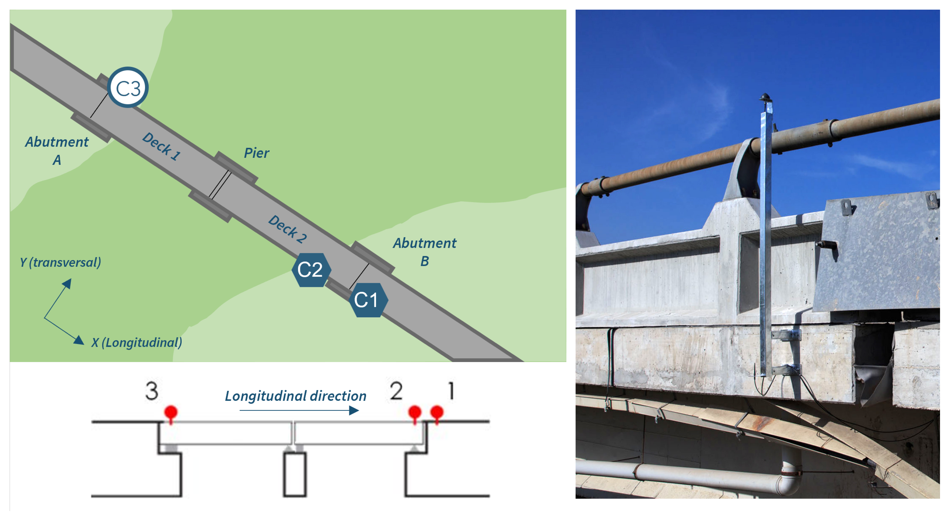
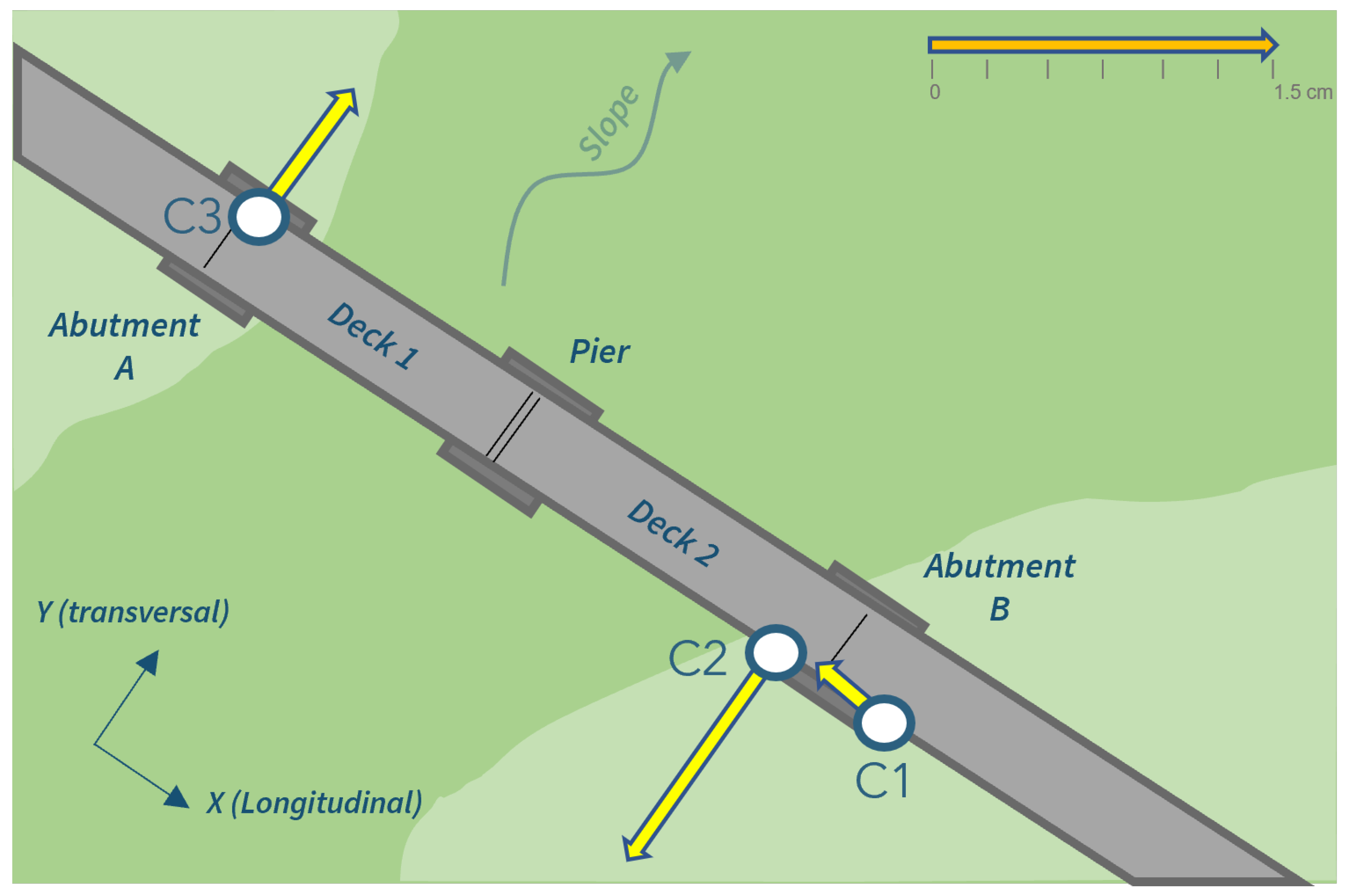
The local monitoring network is composed of only three stations (called C1, C2 and C3) placed in such a way as to have information on the longitudinal deformation (bases C1–C3 and C2–C3) as well as on the relative transversal motion between a pier and a deck. The position of the points is illustrated in Figure 4. The three stations started operating in February 2016. As a matter of fact, the design was enriched with three additional stations located on the central pier in 2020; however, we will examine only the smaller network, for which a full data set that is about 4 years long is available.
As can be seen in Figure 4, the mounting of the antennas brings them above the level of the bridge in order to guarantee better sky visibility.
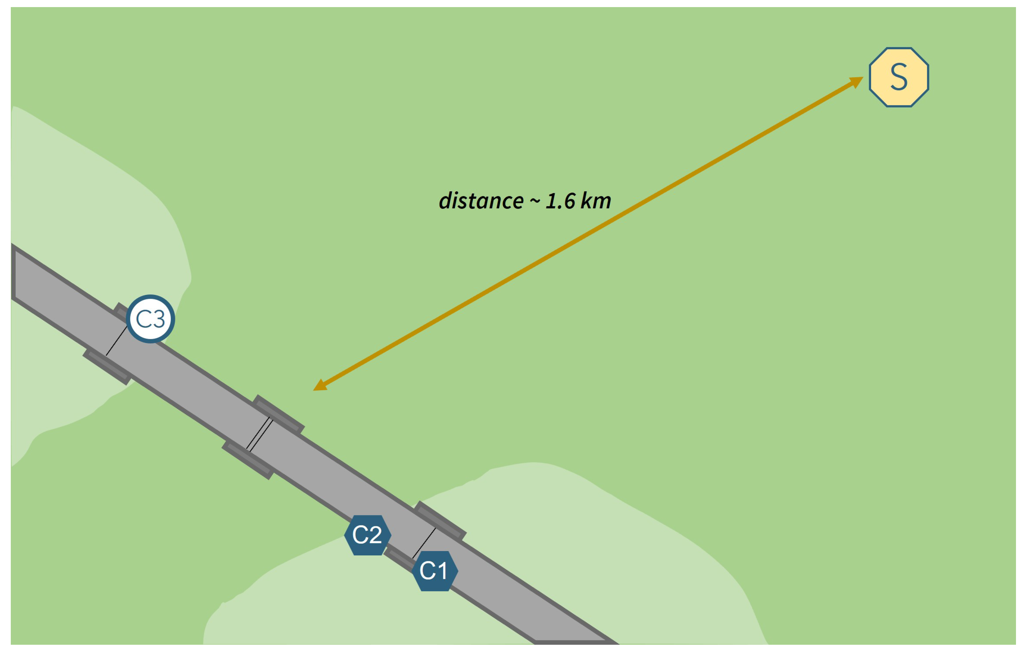
This small local network has been analyzed locally to display its internal differential motion. C3 has been chosen as the master station, and the origin of a Cartesian system has been fixed there; however, any of the three stations may be used as a local master. The X-axis is directed along the bridge, the Y-axis is transversal, and the Z-axis is vertical. Beyond these three points, the monitoring network can be considered to include another permanent geodetic station S, part of the geodetic Italian network, 2 km from the bridge. The use of S as reference, although providing noisier positions, is quite useful for finding long-term motions of the bridge with respect to its environment, as we will see in Section 3.6.

3.4. Hardware and Software

The stations deployed on the bridge are called GeoGuard Monitoring Units (GMU). They have been specifically designed and realized by GReD and algoWatt for monitoring applications in different contexts.
They are schematically composed of:
  • Tallysman GNSS antenna and cables;
  • Solar panel (30 W, 50 W, or 80 W) to provide electric power when it is not available on site;
  • Box containing a battery (providing autonomy for 5–7 days), a GNSS receiver, memory and a transmission apparatus (based on u-blox SARA-U201 module);
  • Low-cost, single-frequency, multi-constellation GNSS receiver (u-blox NEO-M8T) or low-cost, dual-frequency, multi-constellation GNSS receiver (u-blox ZED-F9T).
Data are accumulated and transmission is usually performed every 5 or 15 min; in case one transmission fails, it is repeated at the next slot. Data are received by the GeoGuard analysis center, are identified and validated, and are then passed to the computing engine, which is in charge of estimating the positions of the points with a chosen latency, in this case, daily or hourly. All the data discussed in the paper have been processed by GReD using its own proprietary GNSS software, Breva®.
Results are then collected and provided to the customer in digital and graphical form in a dedicated area of the GeoGuard system. If anomalous motion is detected, a warning and, in the case of persistence, an alarm are issued in the data center and are shared by email, instant messaging applications and/or SMS. The types of solutions presently provided as a continuous service are summarized in Table 1.

3.5. Results of Relative Motion

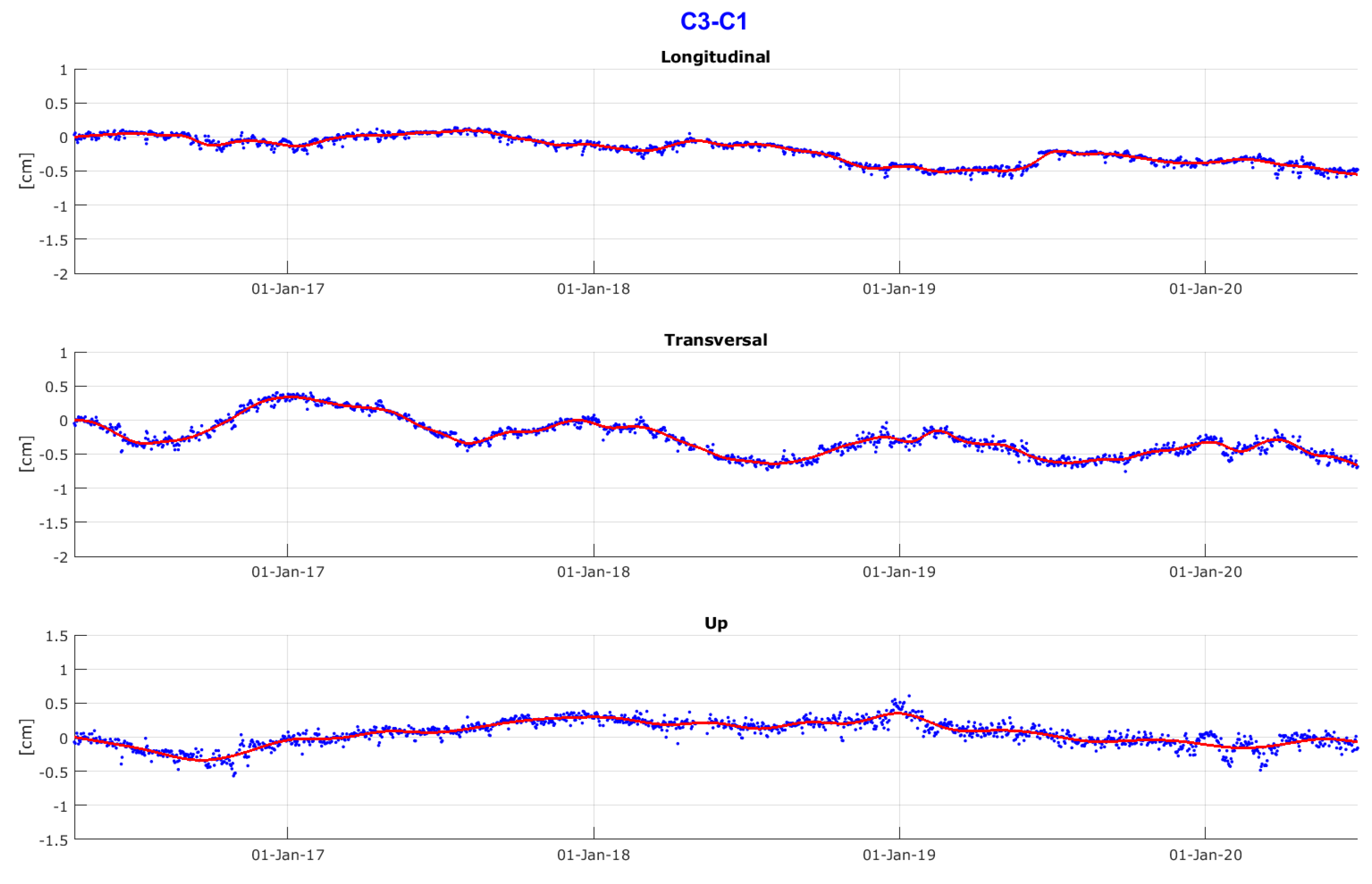
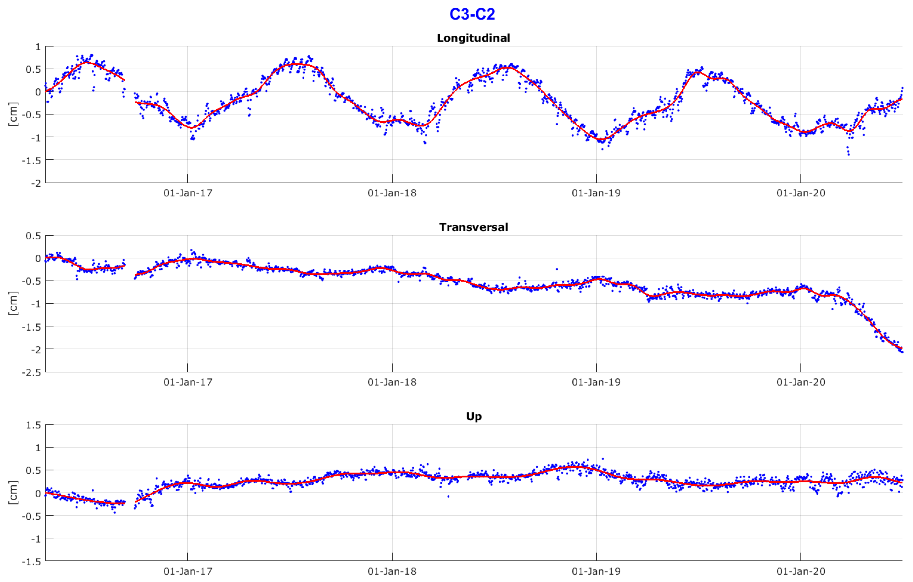
In Figure 5 and Figure 6, we present the daily solutions of the positioning of C1 and C2 with respect to C3 for a time-span of about 4 years. Note that the first day’s solutions are taken as the origin, i.e., only variations are plotted. The first remark is that there is quite a clear separation between the “slow” mean motion, interpolated by cubic splines and represented by the red curves in the figures, and the essentially random oscillations of the daily solutions around the former. The r.m.s. of the residuals is summarized in the following table.
The σ X figure in Table 2 is reduced to 0.5 mm by using a 3-day spline that better describes a shorter period motion.
A second comment is that there is a substantial difference between the behavior of the mean motion for the the bases:
  • C3–C1: very little motion of at most ∼1 cm over the 4 years in all the coordinates, a long-term very small negative trend in X and Y;
  • C3–C2: marked seasonal signal with an amplitude of ∼2 cm in X (longitudinal) with clear annual periodicity;
  • C3–C2: very small negative trend in Y up to March 2020, followed by a descent during springtime, a period in which ASPI had been working on the bridge. Although it is not covered by the displayed data, it is possible to prove stabilization of the descent after about 3 months;
  • C3–C2: essential stability in Z with a pattern very similar to that of C3–C1.
The reason why the signal is present in C3–C2 and not in C3–C1 is structural. C3 is fixed to Abutment A (Figure 4), while C2 is on the extreme of Deck 2, which is constrained to the middle pier and free to move on Abutment B, as described in Section 3.3. On the contrary, C1 is tied to Abutment B.
The origin of the period of the signal in X (longitudinal) of the base C3–C2 is essentially related to the seasonal oscillation of the temperature of the structure, as we prove later. Temperatures have been measured by a thermometer embedded in the structure. This signal is clearly more important in the longitudinal direction, which is also the direction of the base, than in the transversal direction. Thus, the oscillation of X (longitudinal) in C3–C2 represents the thermal linear elongation of the structure of the bridge over a length of about 32 m.
To corroborate this statement, we can compare the plot of X of C3–C2 with that of the mean daily temperature of the bridge. Apart from the visual agreement, we find a correlation coefficient of ρ = 0.95 , which is quite significant. Furthermore an elementary linear regression of Δ X i = x i x ¯ over Δ T i = T i T ¯ gives a linear regression coefficient
a = E ( Δ X i Δ i ) E ( Δ T i 2 ) = 0.000473   mK 1
which, divided by the length of Deck 2, provides the mean thermal expansion coefficient
α = 1.48 × 10 5   K 1
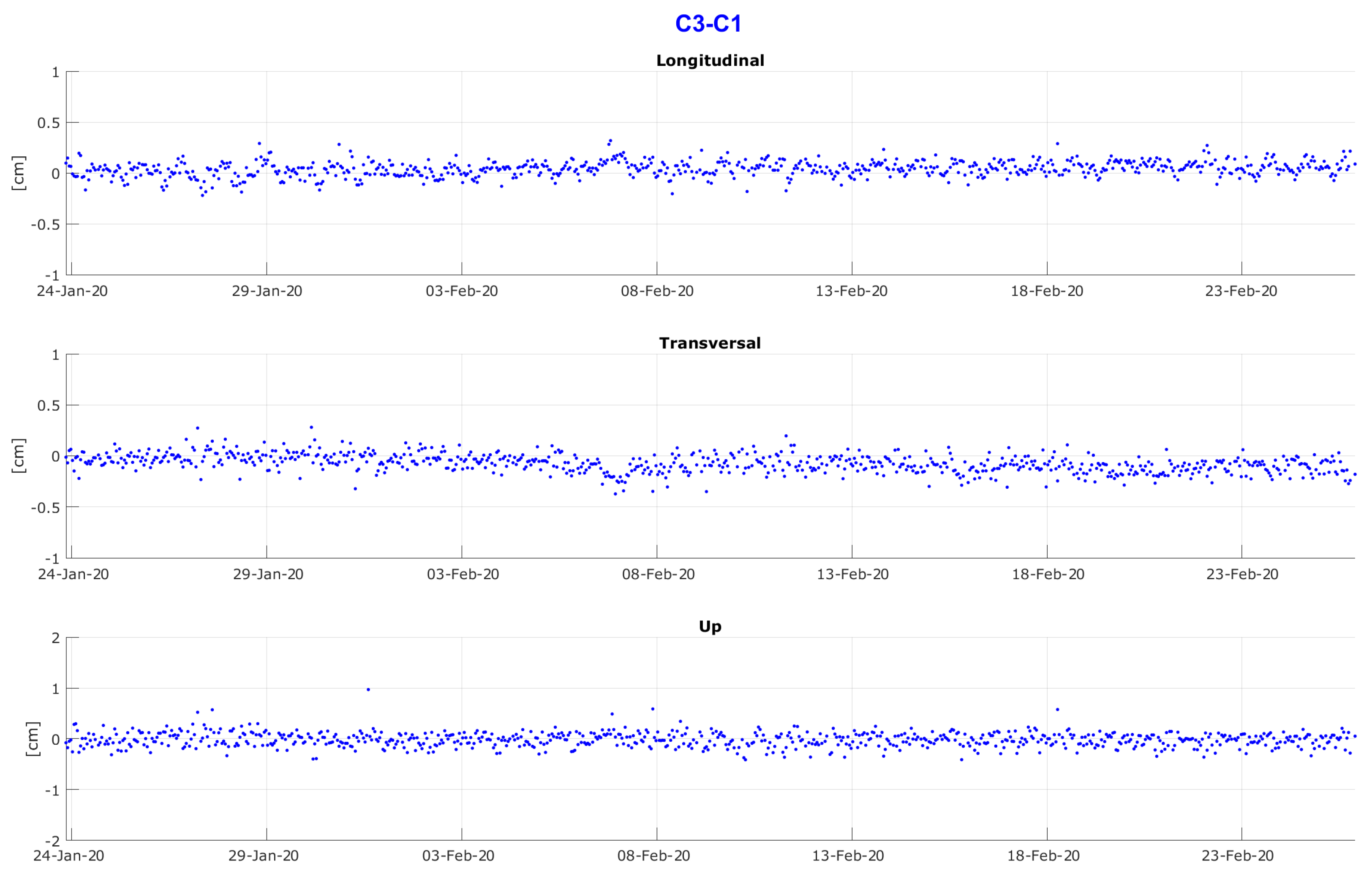
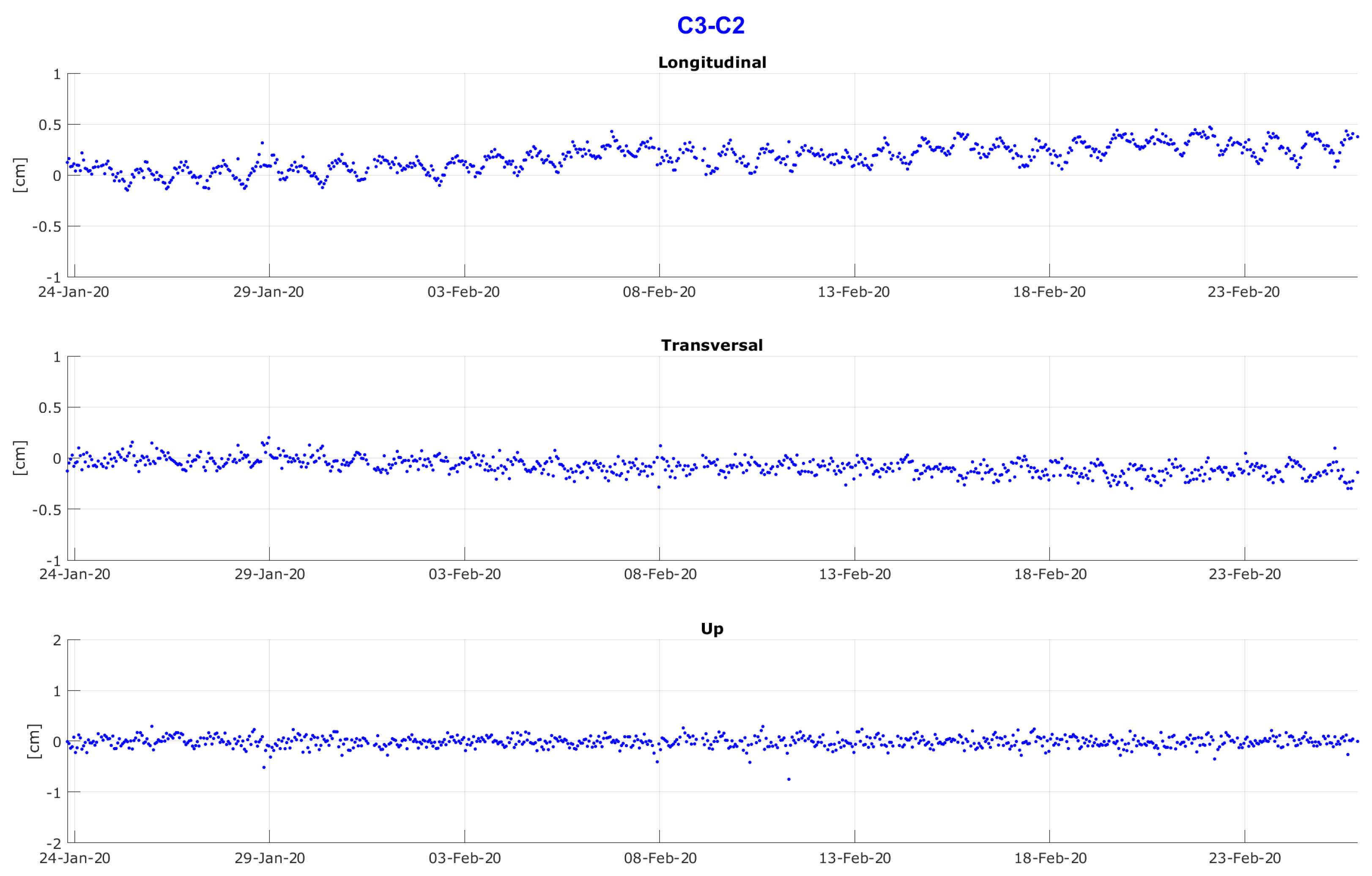
Finally, in Figure 7 and Figure 8, we present the hourly solutions of the two bases, C3–C1 and C3–C2, over a period of 1 month. The first remark is that the series are quite noisier than those of daily solutions, as can be verified from Table 3.
On the other hand, in the horizontal coordinates X and Y, there now appears a quite clear periodic signal with a daily period and a mean oscillation of about 4 mm; this will be discussed in Section 4.

3.6. Results of the Absolute Motion

The permanent station S (Figure 9), which is 1.6 km away from the bridge and is framed in the global ITRF system, has been used to compute the absolute displacements.
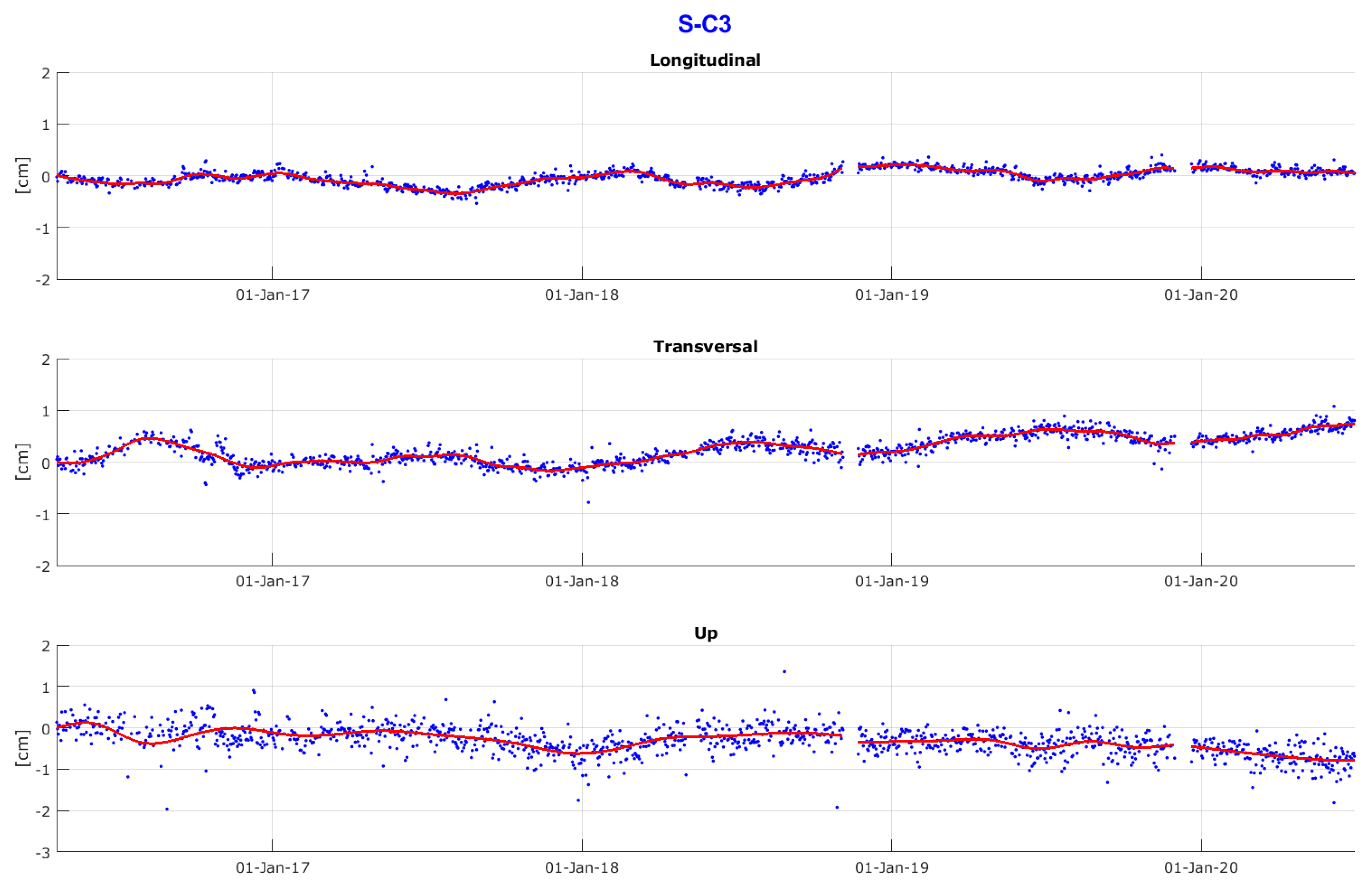
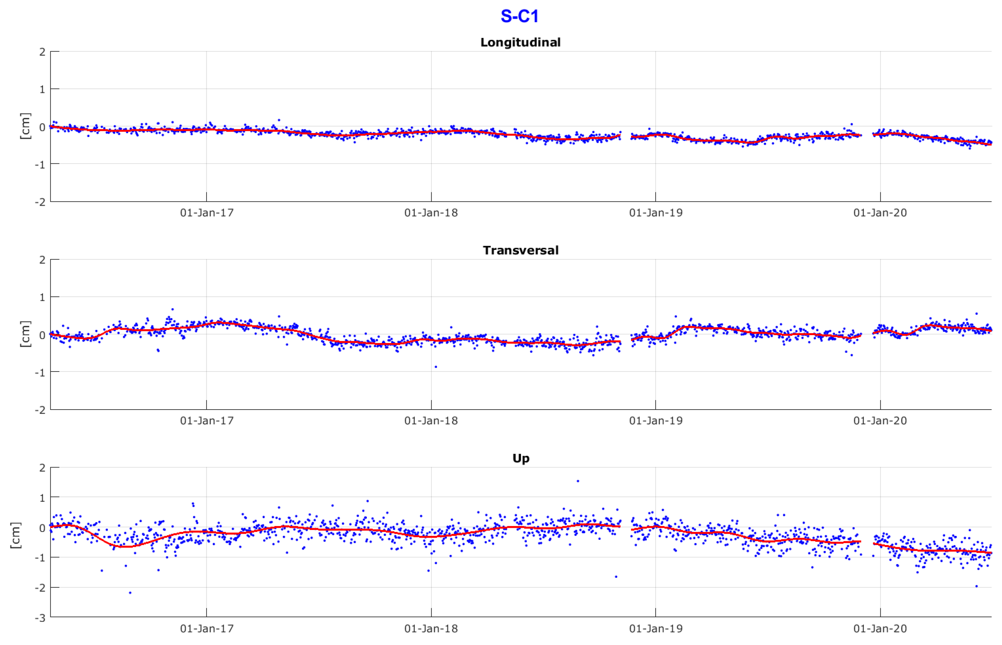
The time series of the coordinates of S with respect to other permanent stations in the area included in the International Terrestrial Reference Frame allows for careful monitoring of the stability of the reference station. In Figure 10, Figure 11 and Figure 12, we present the time series of the shifts of the three stations, C1, C2, and C3, with respect to the permanent station S. Therefore, we interpret the plots of Figure 10, Figure 11 and Figure 12 as the motion of the bridge with respect to the surrounding area, say, of some tens of kilometers of diameter.
The first remark we can make on Figure 10, Figure 11 and Figure 12 is that the estimates of the longer bases, S–C3, S–C1, and S–C2, are significantly noisier than those of the very short baselines on the bridge, as expected. This is confirmed by numbers in Table 4.
Next, we can analyze the plot in Figure 10 to study the absolute motion of our local reference C3.
The series in X of C3 (Figure 10) shows a non-significant trend of a couple of millimeters over 4 years, while Y has a more important trend of about 8 mm over 4 years. To better understand this motion, we plotted the shift in the horizontal plane with the Y-axis along the steepest descent direction of the slope (Figure 13).
As can be seen, in this system, we find that the motion of C3 is only in the slope direction. More accurate analysis shows that the motion presents mostly in the years 2018–2019, while it slows down in later years. Corresponding to the sliding of C3 towards the valley, we also see motion of C2 in the uphill direction, displaying a possible clockwise rotation of the structure in the horizontal plane.
The behavior of C3 in the up direction is interesting; in fact, though much noisier, the plot shows a clear subsidence of about 1 cm in 4 years. Even more interesting is that a subsidence almost coinciding with that of C3 is found in the plots of C1 (Figure 11) and C2 (Figure 12). This also demonstrates the importance of framing the local intrinsic network within a larger network of permanent stations so that parallel motion of the structure with respect to the surrounding area can be revealed. Another important remark regards the plot of the X time series of C2 (Figure 12), where the thermal oscillation is again fairly visible.
Given that C3 does not move so much in X, it is not surprising that we again find an oscillation of about 1.5 cm, as in Figure 6.

4. Discussion and Perspectives

4.1. Discussion

The observational model of the GNSS phases contains so many factors that when trying to interpret time variations of the estimated coordinates of a station, one is always in doubt as to which factor is the origin of the variation. Thus, interpretation of the adjusted coordinates of the station needs some considerations coming from outside the information of the phase measurement alone. We have already seen, for instance, that the signal in X on the base C3–C2 has a clear correlation with the temperature (Figure 8), but it is not known whether the temperature produces elongation on the basis of expansion of the deck or via tropospheric correction, which is usually neglected for such short bases. The answer comes from a combination of different considerations: structurally, point C2 is clamped to Deck 2, which is leaning on a pier and, to some extent, is free to move in the longitudinal direction of the bridge; if the effect was due to imperfect modeling of tropospheric effects, a similar signal should be present in the base C3–C1, which is very close to the other base. In addition, the longer basis S–C2 should be much more affected by tropospheric bias, while the signal in the “absolute” position of C2 displays a signal very similar to that of the “relative” position.
Moreover, the thermal expansion coefficient α estimated in the previous section has a value quite comparable to that of reinforced concrete. All these factors point in the direction of confirming that the phenomenon seen as variations of components of the base is, in fact, thermic elongation. This is important because in a step in the post analysis we can identify it and get information on the structural behavior of the bridge. Further, by removing this component, one is left with a smoother series, i.e., with smaller residuals that give an obvious advantage from the point of view of monitoring interpretation.
Coming to the hourly solutions for C3–C2, we again find a periodic signal in longitudinal direction along the bridge length that is strongly correlated to the daily temperature excursion. Once more, comparison with C3–C1 excludes a tropospheric origin, and we ascribe it to thermal expansion.
We can observe that in the hourly solution, the Z component of both C3–C1 and C3–C2 seems to contain a periodic signal, too, although it is affected by more noise. The two signals in this case have a similar pattern, which is not surprising considering that structurally, so to speak, one station is leaning on the other. We presume, therefore, that this last signal is a common shift due to thermal expansion of the pier on which both C1 and C2 are leaning.

4.2. Perspectives

This long experiment of GNSS monitoring of a bridge suggests three lines of improvement that we briefly describe:
  • We strive to shorten the time unit of adjustments by going to 15–30 min in such a way as to improve latency while still remaining with RMS under 1 cm.
  • Parallel experiments show that it is possible to combine GNSS observations with other sources of data, primarily inclinometers, to improve the monitoring capability of the system. Further, an external source of information, such as SAR, can be integrated into a unique solution.
  • We expect that future data from monitoring sites will be endowed with specific expert systems that also combine completely different information, such as temperatures (of the air and the structure), the level of rain by pluviometers placed near the structure, and other ancillary variables such as the level of water of a river the bridge is crossing, or the level of water of an artificial lake barring the monitored dam.
Thus, the monitoring practice seems to be subject of quite interesting technological and scientific developments in the near future.

Author Contributions

Conceptualization, all authors; methodology, F.S., S.C. and S.B.; software, S.C.; validation, S.C. and S.B.; data curation, L.P.; writing—original draft preparation, F.S. and S.C.; writing—review and editing, L.P., S.C. and S.B. All authors have read and agreed to the published version of the manuscript.

Funding

This research received no external funding.

Institutional Review Board Statement

Not applicable.

Informed Consent Statement

Not applicable.

Data Availability Statement

Not applicable.

Acknowledgments

The authors acknowledge Autostrade per l’Italia SpA, algoWatt SpA and GReD Srl for the effective and enthusiastic cooperation in providing data and supporting the described experience.

Conflicts of Interest

The authors declare no conflict of interest.

Abbreviations

The following abbreviations are used in this manuscript:
ASPIAutostrade per l’Italia
GNSSGlobal Navigation Satellite System
GPSGlobal Positioning System
GReDGeomatics Research & Development
RMSRoot Mean Square
SARSynthetic Aperture Radar

References

  1. DeLoach, S.R. Continuous deformation monitoring with GPS. J. Surv. Eng. 1989, 115, 93–110. [Google Scholar] [CrossRef]
  2. Bock, Y.; Shimada, S. Continuously monitoring GPS networks for deformation measurements. In Global Positioning System: An Overview; Springer: New York, NY, USA, 1990; pp. 40–56. [Google Scholar]
  3. Lovse, J.; Teskey, W.; Lachapelle, G.; Cannon, M. Dynamic deformation monitoring of tall structure using GPS technology. J. Surv. Eng. 1995, 121, 35–40. [Google Scholar] [CrossRef]
  4. Hudnut, K.W.; Behr, J.A. Continuous GPS monitoring of structural deformation at Pacoima Dam, California. Seismol. Res. Lett. 1998, 69, 299–308. [Google Scholar] [CrossRef]
  5. Reguzzoni, M.; Rossi, L.; De Gaetani, C.I.; Caldera, S.; Barzaghi, R. GNSS-Based Dam Monitoring: The Application of a Statistical Approach for Time Series Analysis to a Case Study. Appl. Sci. 2022, 12, 9981. [Google Scholar] [CrossRef]
  6. Fujino, Y.; Murata, M.; Okano, S.; Takeguchi, M. Monitoring system of the Akashi Kaikyo Bridge and displacement measurement using GPS. In Proceedings of the Nondestructive Evaluation of Highways, Utilities, and Pipelines IV, SPIE, Newport Beach, CA, USA, 9 June 2000; Volume 3995, pp. 229–236. [Google Scholar]
  7. Kaloop, M.R.; Li, H. Monitoring of bridge deformation using GPS technique. KSCE J. Civ. Eng. 2009, 13, 423–431. [Google Scholar] [CrossRef]
  8. Watson, C.; Watson, T.; Coleman, R. Structural monitoring of cable-stayed bridge: Analysis of GPS versus modeled deflections. J. Surv. Eng. 2007, 133, 23–28. [Google Scholar] [CrossRef]
  9. Bianchi, S.; Biondini, F.; Anghileri, M.; Capacci, L.; Rosati, G.; Cazzulani, G.; Caldera, S. GNSS-based structural monitoring of the Isola Dovarese Bridge, Italy. In Bridge Safety, Maintenance, Management, Life-Cycle, Resilience and Sustainability; CRC Press: Barcelona, Spain, 11–15 July 2022; pp. 1857–1863. [Google Scholar]
  10. Roberts, G.W.; Meng, X.; Dodson, A.H. Integrating a global positioning system and accelerometers to monitor the deflection of bridges. J. Surv. Eng. 2004, 130, 65–72. [Google Scholar] [CrossRef]
  11. Meng, X.; Roberts, G.W.; Dodson, A.H.; Ince, S.; Waugh, S. GNSS for structural deformation and deflection monitoring: Implementation and data analysis. In Proceedings of the 3rd IAG/12th FIG Symposium, Baden, Germany, 22–24 May 2006; pp. 22–24. [Google Scholar]
  12. Barzaghi, R.; Reguzzoni, M.; De Gaetani, C.I.; Caldera, S.; Rossi, L. Cultural heritage monitoring by low-cost gnss receivers: A feasibility study for san gaudenzio’s cupola, novara. Int. Arch. Photogramm. Remote Sens. Spat. Inf. Sci. 2019, XLII-2/W11, 209–216. [Google Scholar] [CrossRef] [Green Version]
  13. Šegina, E.; Peternel, T.; Urbančič, T.; Realini, E.; Zupan, M.; Jež, J.; Caldera, S.; Gatti, A.; Tagliaferro, G.; Consoli, A.; et al. Monitoring surface displacement of a deep-seated landslide by a low-cost and near real-time GNSS system. Remote Sens. 2020, 12, 3375. [Google Scholar] [CrossRef]
  14. Crosetto, M.; Luzi, G.; Monserrat, O.; Barra, A.; Cuevas-González, M.; Palamá, R.; Krishnakumar, V.; Wassie, Y.; Mirmazloumi, S.M.; Espín-López, P.; et al. Deformation monitoring using sar interferometry and active and passive reflectors. Int. Arch. Photogramm. Remote Sens. Spat. Inf. Sci. 2020, XLIII-B3-2020, 287–292. [Google Scholar] [CrossRef]
  15. Luzi, G.; Espín-López, P.F.; Mira Pérez, F.; Monserrat, O.; Crosetto, M. A Low-Cost Active Reflector for Interferometric Monitoring Based on Sentinel-1 SAR Images. Sensors 2021, 21, 2008. [Google Scholar] [CrossRef] [PubMed]
  16. Delo, G.; Civera, M.; Lenticchia, E.; Miraglia, G.; Surace, C.; Ceravolo, R. Interferometric Satellite Data in Structural Health Monitoring: An Application to the Effects of the Construction of a Subway Line in the Urban Area of Rome. Appl. Sci. 2022, 12, 1658. [Google Scholar] [CrossRef]
  17. Caldera, S.; Realini, E.; Reguzzoni, M.; Sampietro, D.; Sansò, F. GeoGuard: Un nuovo servizio di monitoraggio geodetico per l’osservazione di segnali geodinamici. In Proceedings of the 34° Convegno Nazionale GNGTS, Luglioprint, Trieste, Italy, 17–19 November 2015; pp. 83–88. [Google Scholar]
  18. Caldera, S.; Realini, E.; Barzaghi, R.; Reguzzoni, M.; Sansò, F. Experimental study on low-cost satellite-based geodetic monitoring over short baselines. J. Surv. Eng. 2016, 142, 04015016. [Google Scholar] [CrossRef]
  19. Sampietro, D.; Caldera, S.; Capponi, M.; Realini, E. Geoguard-An innovative technology based on low-cost GNSS receivers to monitor surface deformations. In Proceedings of the First EAGE Workshop on Practical Reservoir Monitoring, Amsterdam, The Netherlands, 6–9 March 2017; European Association of Geoscientists & Engineers: Amsterdam, The Netherlands, 2017; p. 505. [Google Scholar]
  20. Tagliaferro, G.; Caldera, S.; Realini, E.; Molinari, D.; Pasqui, L. GeoGuard: Low-cost GNSS technologies for the continuous monitoring of structures and land movements. In Proceedings of the EGU General Assembly Conference Abstracts, Vienna, Austria, 8–13 April 2018; p. 13898. [Google Scholar]
  21. Altamimi, Z.; Boucher, C.; Sillard, P. New trends for the realization of the International Terrestrial Reference System. Adv. Space Res. 2002, 30, 175–184. [Google Scholar] [CrossRef]
  22. Altamimi, Z.; Rebischung, P.; Métivier, L.; Collilieux, X. ITRF2014: A new release of the International Terrestrial Reference Frame modeling nonlinear station motions. J. Geophys. Res. Solid Earth 2016, 121, 6109–6131. [Google Scholar] [CrossRef] [Green Version]
  23. Tagliaferro, G.; Caldera, S. Impact of Double Differences Correlation on the Adjustment of Small GNSS Networks. J. Surv. Eng. 2019, 145, 04019002. [Google Scholar] [CrossRef]
  24. Hofmann-Wellenhof, B.; Lichtenegger, H.; Collins, J. Global Positioning System: Theory and Practice; Springer Science & Business Media: Vienna, Austria, 2012. [Google Scholar]
  25. Leick, A.; Rapoport, L.; Tatarnikov, D. GPS Satellite Surveying; John Wiley & Sons: Hoboken, NJ, USA, 2015. [Google Scholar]
  26. Teunissen, P.J.; Montenbruck, O. Springer Handbook of Global Navigation Satellite Systems; Springer: Cham, Switzerland, 2017; Volume 10. [Google Scholar]
  27. Sansò, F.; Betti, B.; Albertella, A. Positioning. Posizionamento Classico e Satellitare; CittàStudi Edizioni: Milan, Italy, 2019. [Google Scholar]
  28. Kouba, J. A Guide to Using International GNSS Service (IGS) Products. 2009. Available online: https://kb.igs.org/hc/en-us/articles/201271873-A-Guide-to-Using-the-IGS-Products (accessed on 30 October 2022).
  29. Johnston, G.; Riddell, A.; Hausler, G. The international GNSS service. In Springer Handbook of Global Navigation Satellite Systems; Springer: Cham, Switzerland, 2017; pp. 967–982. [Google Scholar]
  30. Bengio, Y. Learning Deep Architectures for AI; Now Publishers Inc.: Delft, The Netherlands, 2009. [Google Scholar]
  31. LeCun, Y.; Bengio, Y.; Hinton, G. Deep learning. Nature 2015, 521, 436–444. [Google Scholar] [CrossRef] [PubMed]
  32. Ruder, S. An overview of gradient descent optimization algorithms. arXiv 2016, arXiv:1609.04747. [Google Scholar]
  33. Cox, D.R.; Hinkley, D.V. Theoretical Statistics; CRC Press: Boca Raton, FL, USA, 1979. [Google Scholar]
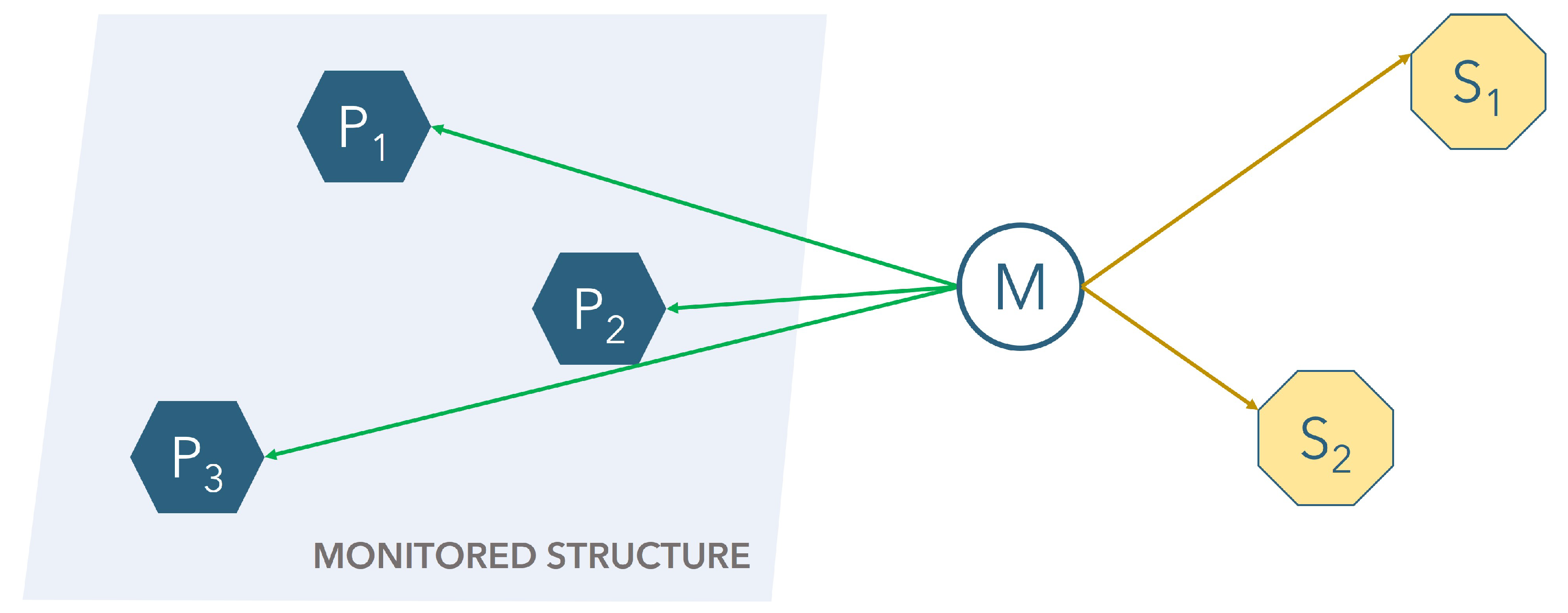
Figure 1. The star-shaped design of a monitoring network; M master station; P 1 , P 2 , P 3 monitored points; and S 1 , S 2 permanent stations of a global positioning service.
Applsci 12 12468 g001
Figure 2. The difference of geometry-free combination between two closed GNSS stations after subtracting the average. GNSS receivers are u-blox.
Applsci 12 12468 g002
Figure 3. Hourly estimates of the coordinates of a point on a bridge: red dots are GPS-only solutions; blue dots are GPS and Galileo joint solutions. Outliers are quite evident.
Applsci 12 12468 g003
Figure 4. Monitoring network deployed on the bridge, together with an example of installation.
Applsci 12 12468 g004
Figure 5. Daily solutions of C3–C1 baseline.
Applsci 12 12468 g005
Figure 6. Daily solutions of C3–C2 baseline.
Applsci 12 12468 g006
Figure 7. Hourly positions of C3–C1 baseline.
Applsci 12 12468 g007
Figure 8. Hourly positions for C3–C2 baseline.
Applsci 12 12468 g008
Figure 9. Conceptual scheme showing the position of permanent station S with respect to the monitoring network on the bridge. The aspect ratio is not maintained.
Applsci 12 12468 g009
Figure 10. Baseline S–C3.
Applsci 12 12468 g010
Figure 11. Baseline S–C1.
Applsci 12 12468 g011
Figure 12. Baseline S–C2.
Applsci 12 12468 g012
Figure 13. X and Y components on the baseline S–C3 with the X-axis oriented along the steepest descent direction of the slope.
Applsci 12 12468 g013
Table 1. Solutions continuously provided for the monitored bridge.
Time IntervalModalityLatency
1 h (24 solutions per day)Relative15 min after the end of the hour, for early warning
2 h (12 solutions per day)Relative15 min after the end of 2 h, to confirm the warning
24 h (daily solution)Relative/AbsoluteDelivered after midnight
Table 2. Root mean squares (RMSs) of X Y Z with respect to the mean motion (splines every 14 days) for the 2 baselines over the 6-year period.
BaselineLength σ X (Longitudinal) σ Y (Transversal) σ Z (Up)
C3–C169.1 m0.4 mm0.5 mm0.7 mm
C3–C267.4 m1.1 mm0.6 mm0.7 mm
Table 3. Root mean squares (RMSs) of X Y Z with respect to the mean motion (splines every 14 days) for the 2 baselines over the 1-month period.
BaselineLength σ X (Longitudinal) σ Y (Transversal) σ Z (Up)
C3–C1horiz.: 69.1 m, vertic.: −0.4 m0.7 mm0.8 mm1.4 mm
C3–C2horiz.: 67.4 m, vertic.: −0.4 m0.9 mm0.7 mm1.1 mm
Table 4. Root mean squares (RMSs) of X Y Z with respect to the mean motion (splines every 14 days) for the 3 baselines over the monitoring period.
BaselineLength σ X (Longitudinal) σ Y (Transversal) σ Z (Up)
S–C1horiz.: 2390.5 m, vertic.: −214.6 m0.6 mm1.0 mm2.7 mm
S–C2horiz.: 2390.3 m, vertic.: −214.2 m1.1 mm1.0 mm2.7 mm
S–C3horiz.: 2405.2 m, vertic.: −214.2 m0.6 mm1.0 mm2.6 mm
Publisher’s Note: MDPI stays neutral with regard to jurisdictional claims in published maps and institutional affiliations.