On the Patterns and Scaling Properties of the 2021–2022 Arkalochori Earthquake Sequence (Central Crete, Greece) Based on Seismological, Geophysical and Satellite Observations

Abstract

The 27 September 2021 damaging mainshock (Mw6.0) close to Arkalochori village is the strongest earthquake that was recorded during the instrumental period of seismicity in Central Crete (Greece). The mainshock was preceded by a significant number of foreshocks that lasted nearly four months. Maximum ground subsidence of about 18 cm was estimated from InSAR processing. The aftershock sequence is located in an almost NE-SW direction and divided into two main clusters, the southern and the northern ones. The foreshock activity, the deformation area, and the strongest aftershocks are located within the southern cluster. Based on body-wave travel times, a 3-D velocity model was developed, while using combined space and ground-based geodetic techniques, the co-seismic ground deformation is presented. Moreover, we examined the co-seismic static stress changes with respect to the aftershocks’ spatial distribution during the major events of the foreshocks, the Mw = 6.0 main event as well as the largest aftershock. Both the foreshock and the aftershock sequences obey the scaling law for the frequency-magnitude distribution as derived from the framework of non-extensive statistical physics (NESP). The aftershock production rate decays according to the modified Omori scaling law, exhibiting various Omori regimes due to the generation of secondary aftershock sequences. The analysis of the inter-event time distribution, based on NESP, further indicates asymptotic power-law scaling and long-range correlations among the events. The spatiotemporal evolution of the aftershock sequence indicates triggering by co-seismic stress transfer, while its slow migration towards the outer edges of the area of the aftershocks, related to the logarithm of time, further indicates a possible afterslip.

1. Introduction

Greece is located at the southeastern tip of Europe where a variety of geological processes take place, such as the formation of the Alpine Mountain chain from the Western French Alps to the Dinarides in the Balkan Peninsula due to the collision between European and Nubian plates. Furthermore, observed intense deformation in the Aegean and the surrounding regions produces a significant portion of SE Europe’s seismicity, concentrated in thrust structures along the Hellenic Arc and smaller extensive ruptures in the area of the Aegean back-arc [1,2,3,4].

The epicentral area is located in the front of the Hellenic arc, near the region where the European and Nubia plates converge, giving rise to large earthquakes [1,2,3,4,5]. The most characteristic tectonic features in the vicinity of the rapture zone are the two large tectonic basins located in the northern Heraklion and the southwest Messara. These were formed by extensional forces from an arc-normal pull since 11 Ma which formed the average NNE-SSW direction faults [1,2]. The basins are filled with Miocene to Pliocene sediments overlaid by Quaternary deposits and in the north-eastern part, there are exposed nappes tectonic features consisting of Carbonates of the Tripolis and Trypalion units.

Several field surveys showed the existence of active extensional faults in the upper crust of Crete along both E-W and N-S directions, (e.g., [6,7,8,9,10,11,12]). The 2021 seismic crisis in Arkalochori and the neighboring villages was located in a fault system of what was considered possibly active with NW-SE and NE-SW direction of strike, (e.g., [8,10,11,13,14,15]), bounding the Heraklion basin.

Destructive earthquakes occurred in the broader Crete region during the pre-instrumental era [16,17,18]. In Central Crete, two major historical earthquakes have been reported, both in the vicinity of Heraklion. The first one was on 1 July 1494 (M = 5.4) [16] while on 26 November 1595, a second event (M ~ 6.4) took place, both causing severe damage on the island of Crete [16,18].

On 27 September 2021 an Mw = 6.0 event, linked to an approximately N-S trending normal fault at the central part of the island of Crete, Greece, occurred ~20 km to the south of the prefecture’s capital. The occurrence of the mainshock took place after a long time of foreshocks since the first half of June 2021 with criticality characteristics [19] and a long aftershock sequence with the strongest event occurring on 28 September with local magnitude M_L5.3. Following the recent report by ITSAK [20], the recorded PGA at the epicentral area (Arkalochori) was 0.62 g in the horizontal component (N-S) and 0.82 g in the vertical one, with a duration of strong ground motion (>0.1 g) almost 6 s. Its focal mechanism is characterized by an SSW-NNE to SW-NE-trending, nearly dip-slip normal faulting. Its strike generally ranges from N200° E–N230° E and its dip angle varies between 40° and 60°. The active fault associated with the main event is the Kastelli Fault, which has a progressive change in the strike from 225° to 265° northeastwards and dips between 60°–80° northwestwards [9,21,22,23].

In this work, we present the consistency between seismological, geodetic, satellite, and geophysical data for the 2021–2022 Arkalochori earthquake sequence, highlighting the complementarity of multi-disciplinary approaches. First, we relocate the 2021–2022 Central Crete earthquake sequence to have a more accurate insight on its distribution and scaling properties. Based on body-wave travel times, we have developed a 3D velocity model, while using combined space and ground based geodetic techniques the co-seismic ground deformation is obtained. Moreover, we examined the co-seismic static stress changes with respect to the aftershocks’ spatial distribution during the major events of the foreshocks, the Mw = 6.0 main event as well as the largest aftershock. In addition, the scaling properties of the 2021–2022 Central Crete earthquake sequence are investigated thoroughly and we analyzed the aftershocks decay rate based on the modified-Omori formula. Furthermore, the frequency–magnitude distribution parameters of the earthquake sequence along with that of the distribution of inter-event times between the successive events are viewed in terms of non-extensive statistical physics in order to provide more detailed insights into the complex nature of the long-term correlation of the earthquake generation process.

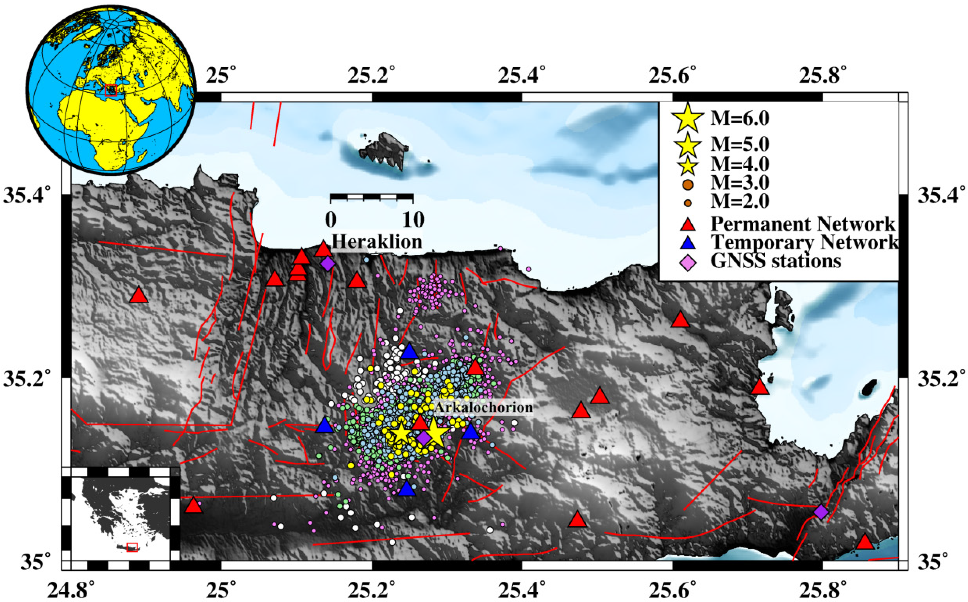
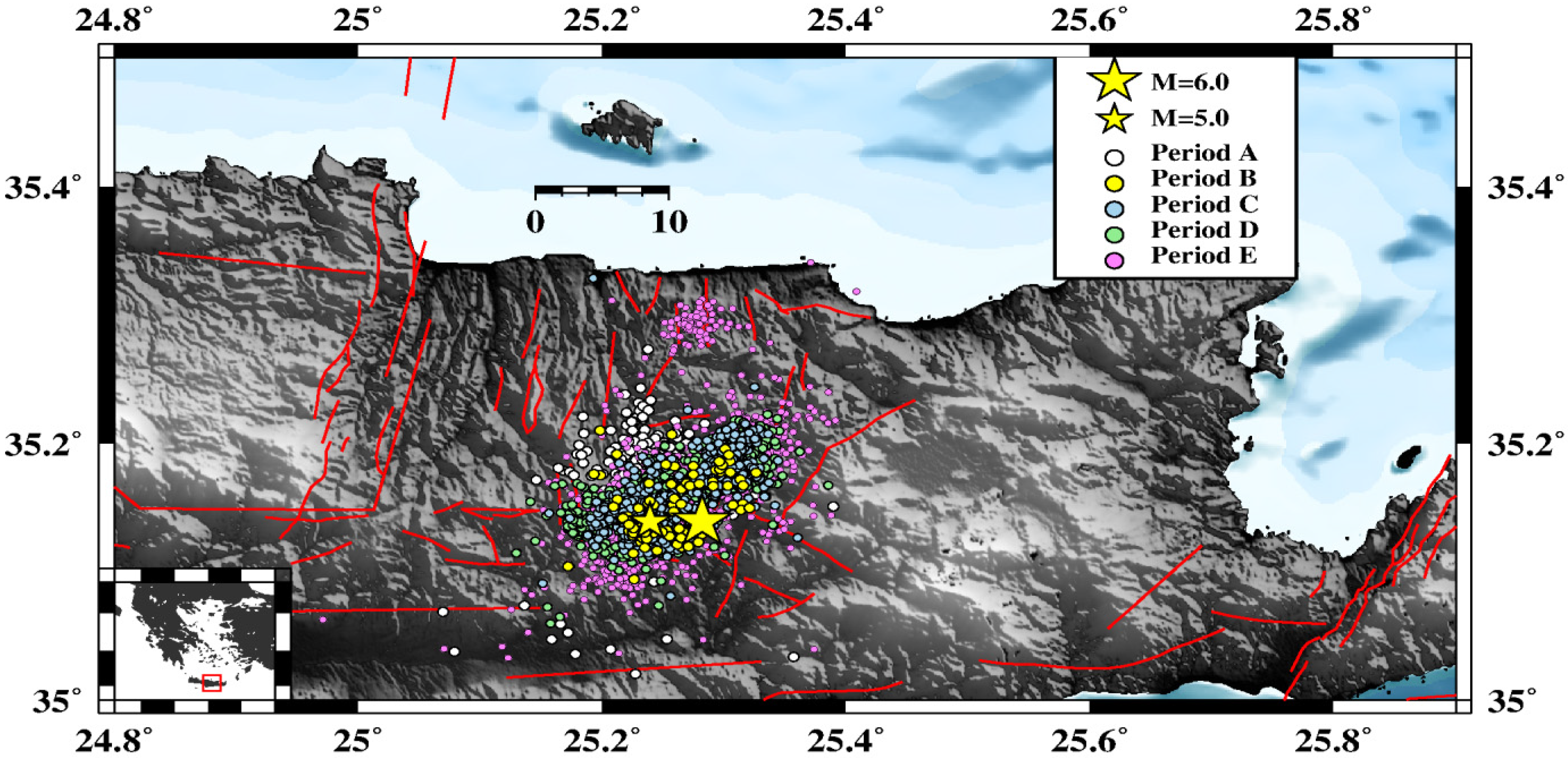
2. Seismological Data and Earthquake Sequence Analysis

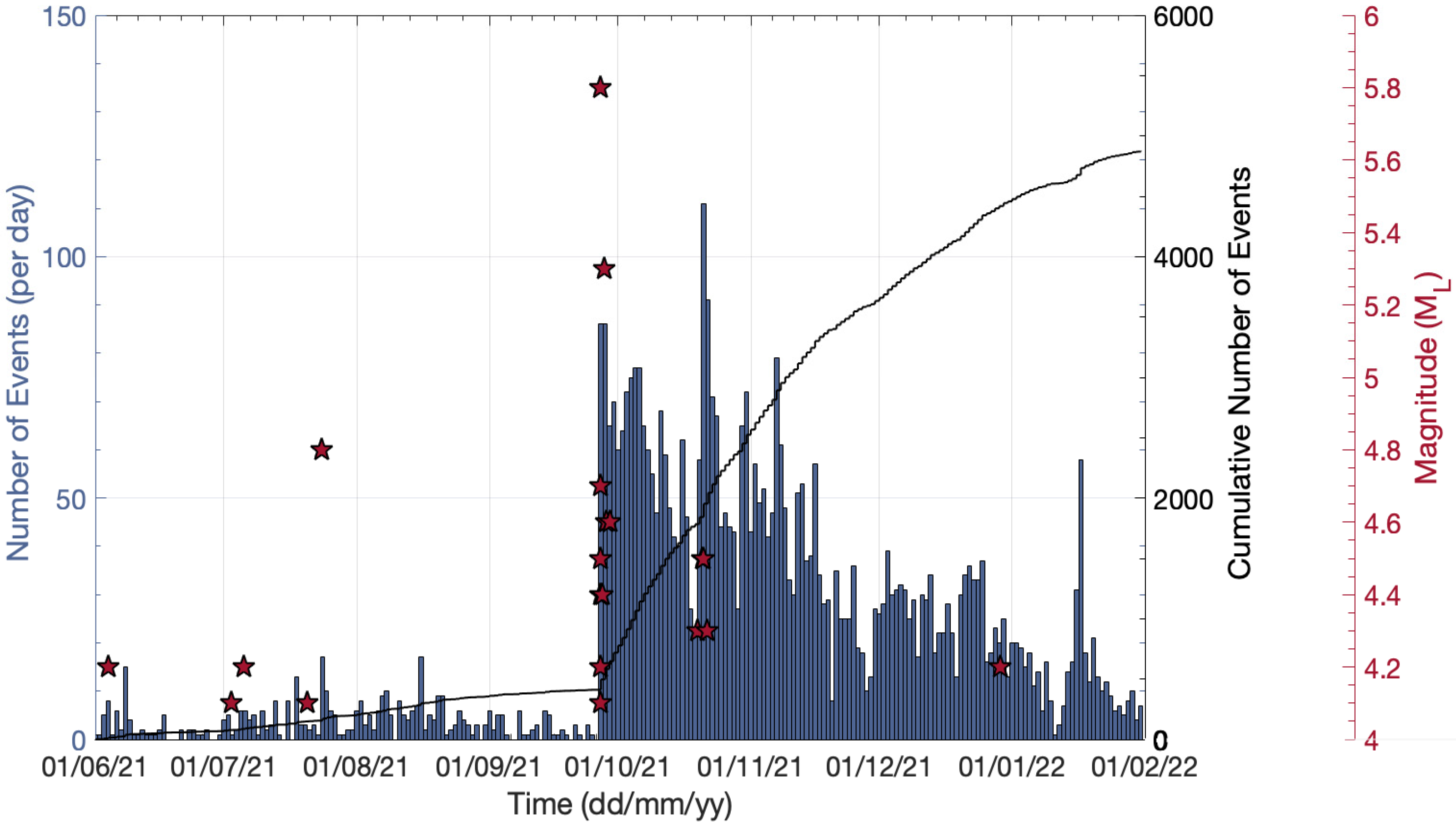
The 2021 seismic crisis in the wider area of Arkalochori began in the form of an earthquake swarm in early June 2021. The situation, however, changed dramatically since the occurrence of the Mw = 6.0 main event on 27 September 2021. Although several permanent stations of the Hellenic Unified Seismological Network operate on the island of Crete at the time of the mainshock, the closest station to the epicentral area was KNSS of the Hellenic Mediterranean University Research Center (HC network at formerly Technological Educational Institute of Crete [24]), at a distance of about 12–22 km. These data were manually revised using a regional 1D model and were put into a relocation procedure in order to obtain more accurate results, as will be discussed in the next sections.

2.1. Data Analysis

The Arkalochori earthquake sequence is divided into two main temporal groups, one that preceded the 27 September Mw = 6.0 mainshock, consisting of 620 events with a significant rise in numbers during July and August 2021, and the aftershock sequence, divided into three sub-groups, composed by 4130 seismic events (Figure 1). A major part of the sequence was recorded by local stations of the regional Hellenic Unified Seismological Network (HUSN), with the nearest stations being KNSS, PFKS (IFEGG), located ~20 km to the SW and NE of the epicenter, respectively. On October 1, 2021, the Geodynamics Institute of the National Observatory of Athens (GI-NOA) installed 4 temporary stations (CRE1–4) around the aftershock zone, contributing to the depth accuracy and providing a preliminary hypocentral solution for this time period.

A total of 4750 events of the 2021–2022 Arkalochori sequence that occurred during the period between 13 January and 31 January 2022 (Figure 2) were detected and manually analyzed using real-time waveform data from the Hellenic Unified Seismological Network (HUSN) in the SeisComP3 graphical user interface [25]. During the first stage of the sequence analysis, hypocenters were located in near real-time, by employing the Hypo71 single-event algorithm [26] and a custom regional 1D velocity model for the Hellenic peninsula [27].

In this study, two local 1D velocity models [28,29] have been used through the second stage of the data processing, running the HypoInverse code [30]. Residual values from these models were compared (

Table 1. Comparison of the error statistics between Model 1 [28] and Model 2 [29] for the Arkalochori seismic sequence.

Model	Model 1	Model 2
Mean RMS (s)	0.26	0.26
Mean ERH (km)	1.30	1.31
Mean ERZ (km)	4.41	4.52
Mean Depth (km)	9.43	13.94

) with no significant differences, while the epicentral differences were less than 0.5 km, whereas the depths, which are more sensitive to the velocity model, differed by about 1 km on average. The [28] velocity model (Model 1) provided much shallower events than the respective ones of [29] (Model 2) and especially for the stronger events of the sequence (Mw = 6.0 and Mw = 5.3) that were located at a depth shallower than 5 km (2.7 and 0.7 km, respectively), which seemed unrealistic in terms of earthquake physics and the past of the area.

The final hypocentral locations were obtained using the velocity model of [29]. The range of depth distribution is mainly between 5 and 15 km for the aftershocks of the 27 September Mw = 6.0 event. Figure 2 presents the distribution of 4750 events that were manually revised and relocated with HypoInverse code, along with the faults in the area as extracted from [31].

The seismic sequence was divided into five sub-groups according to its spatiotemporal occurrence (Figure 3):

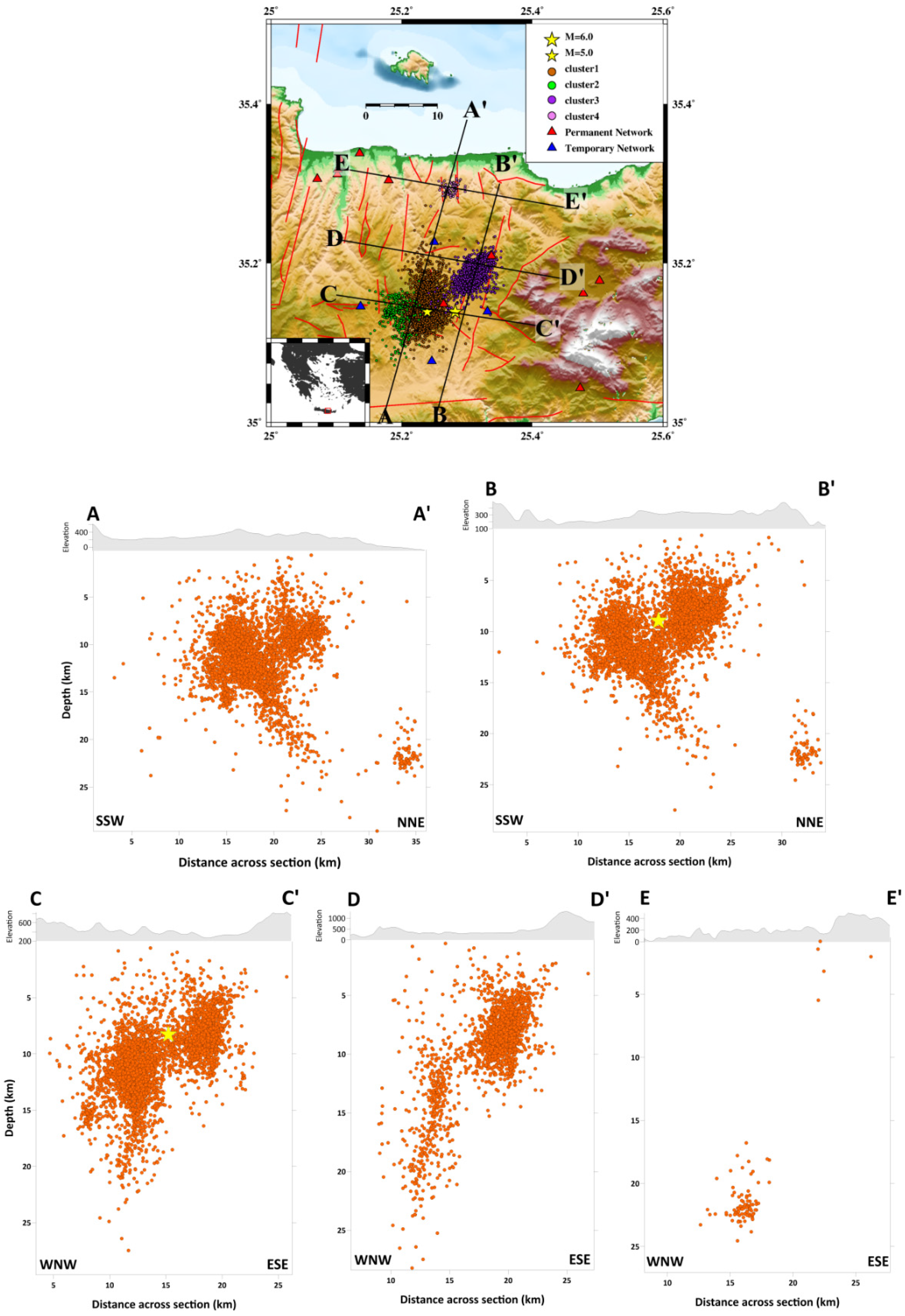
• 13 January–27 September 2021 (period A), consisting of 620 events;
• 27 September–28 September 2021 (period B), the first day of the aftershock sequence and just a few hours before the greatest aftershock (M5.3), composed of 90 events;
• 28 September–12 October 2021 (period C), just after the occurrence of the M = 5.3 aftershock at 04:48 UTC, consisting of 803 events;
• 12 October–31 October 2021 (period D), where the M = 4.0 event took place after a significant decay in the aftershocks number in Arkalochori;
• 1 November–31 January 2022 (period E), which comprises small to moderate magnitude events in a deeper part of the crust (H > 20 km) located near Herakleion.

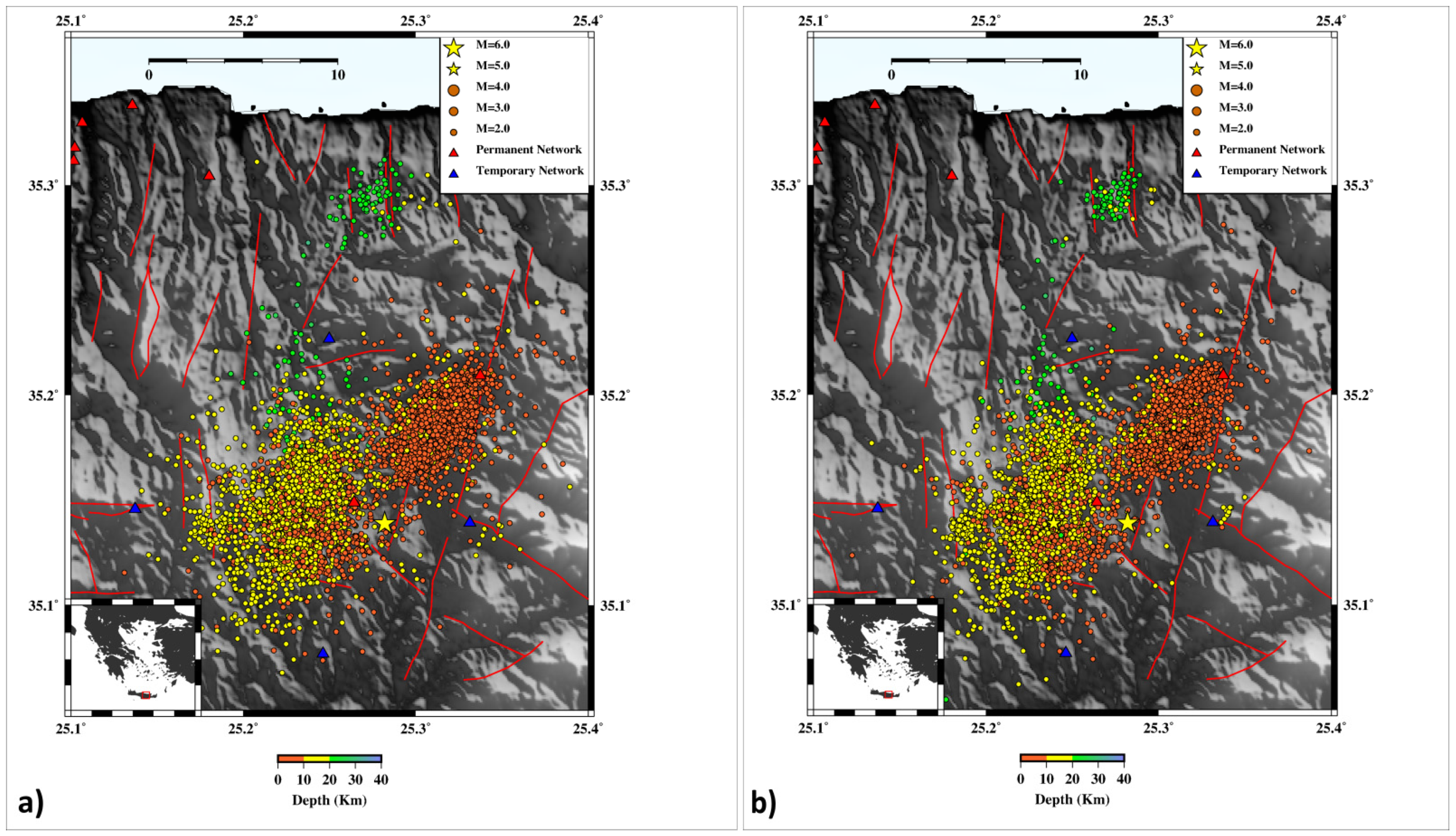
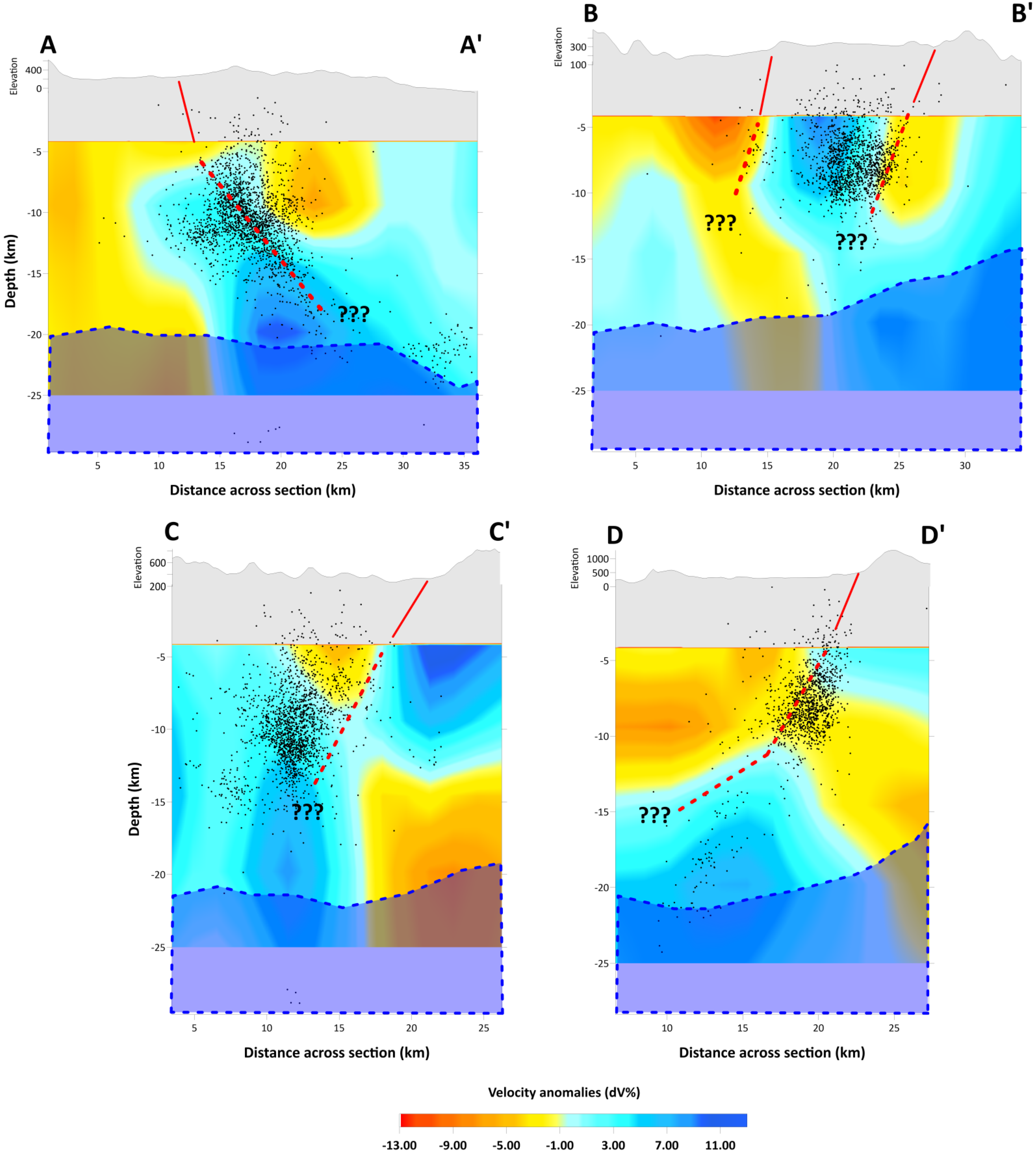
2.2. Hypocentral Relocation of the Earthquake Sequence

Accurate earthquake hypocenter parameters are required in order to obtain a detailed image of the structural properties and processes that trigger seismic activity. The precision of hypocenter locations and their uncertainties depend on several factors, including the number and quality of available seismic phases, the accuracy with which arrival times are measured, the network geometry, the knowledge of the velocity structure, and the linear approximation to a set of non-linear equations, which is assumed in the inversion. hypoDD [32] is an algorithm that reduces residuals between observed and theoretical differences of travel times (or double differences) for pairs of neighboring events at each station that recorded both events, as can be seen from Equation (1). This way, errors due to unmodeled velocity structures are minimized without station corrections. A minimum 1D layered velocity model is used to predict the travel time differences and partial derivatives (Equation (2)).

$$d{r}_k^{ij}={(t_k^i-t_k^j)}^{obs}-{(t_k^i-t_k^j)}^{cal}$$

(1)

$$\frac{\partial t_k^i}{\partial m}\Delta m^i-\frac{\partial t_k^i}{\partial m}\Delta m^j=d{r}_k^{ij}$$

(2)

where m = (x, y, z).

Inter-event distance and misfit weighting are applied to catalog data after the end of each iteration, in order to optimize their quality during the relocation procedure. Horizontal and vertical relative spatial errors can be minimized by approximately one order of magnitude under certain conditions. In this study, more than 4500 events of M_L ≥ 0.6, comprising 58,777 phases, were relocated with hypoDD. Among the main factors that had been taken into consideration during the relocation procedure were the following: (a) network coverage of the area, (b) the size of the dominant clusters, and (c) their maximum separation distance. This led to the formation of 98,070 P- and 43,812 S-phase pairs, respectively, for the whole volume, while in the central cluster (cluster #1), where the mainshock (M = 6.0) largest aftershock (Mw = 5.3) is situated, 98,070 P- and 18,673 S-phase pairs were formed.

In the area of Central Crete, 4728 out of 4750 events of the initial catalog (M ≥ 0.6), were relocated with hypoDD, giving a first result that could be rated as satisfactory. The mean temporal errors (rms) were reduced from 0.14 s to 0.11 s, while the spatial errors (erx, ery, erz) were decreased from 1.0, 0.8, and 2.0 km to 0.3, 0.3, and 0.4 km, respectively (Table 1). The hypoDD-estimated errors in the final locations were calculated using the LSQR method, which may not be representative of the real ones [32].

The epicenter of the mainshock was located less than 3 km to the SE of Arkalochori (lat: 35.1416° N, long: 25.2736° E) at a depth of ~9.6 km, obtained by the double difference algorithm procedure. The optimization of the final results leads to the clustering of the earthquake sequence into four main clusters. A dense cluster of events has occurred west of the mainshock, in an approximately 15 km long area associated with the foreshocks (cluster 1). The epicenters of cluster 2 were mainly distributed in the area between Amourgeles and Parthenio N-S oriented normal faults, in the region to the west of Arkalochori. Further to the NE, another significant cluster of events (cluster 3) was also observed, in the footwall of Agnos NE-SW striking normal fault, near Kastelli (Figure 4). Most seismicity is in a range of focal depths between 7 and 18 km.

Furthermore, five (5) cross-sections were performed in order to see the impact of the relocation procedure on the sequence hypocentral depths and the discrimination of the local activated structures. Cross-sections 1–2 have an NNE-SSW orientation, and 3–5 WNW-ESE direction, perpendicular to the NE trending faults. The geometry of the hypocenters as they appear in the performed cross-sections, reveal the activation of a fault, dipping ~60° to the WNW, and a smaller antithetic structure, possibly connected to Galatas N-S striking normal fault (Figure 5).

An almost sub-vertical structure makes an appearance in the cross-sections north of the epicenter of the mainshock (sections B–B’, D–D’; Figure 5). The earthquake activity that belongs to cluster 4, started on 16 January 2022, with an event of M_L = 3.3 and continued throughout the first two months of 2022 as the latest contribution to the seismic sequence. The hypocenters appear to be located in deeper parts of the crust and they have an apparent dip towards the WNW.

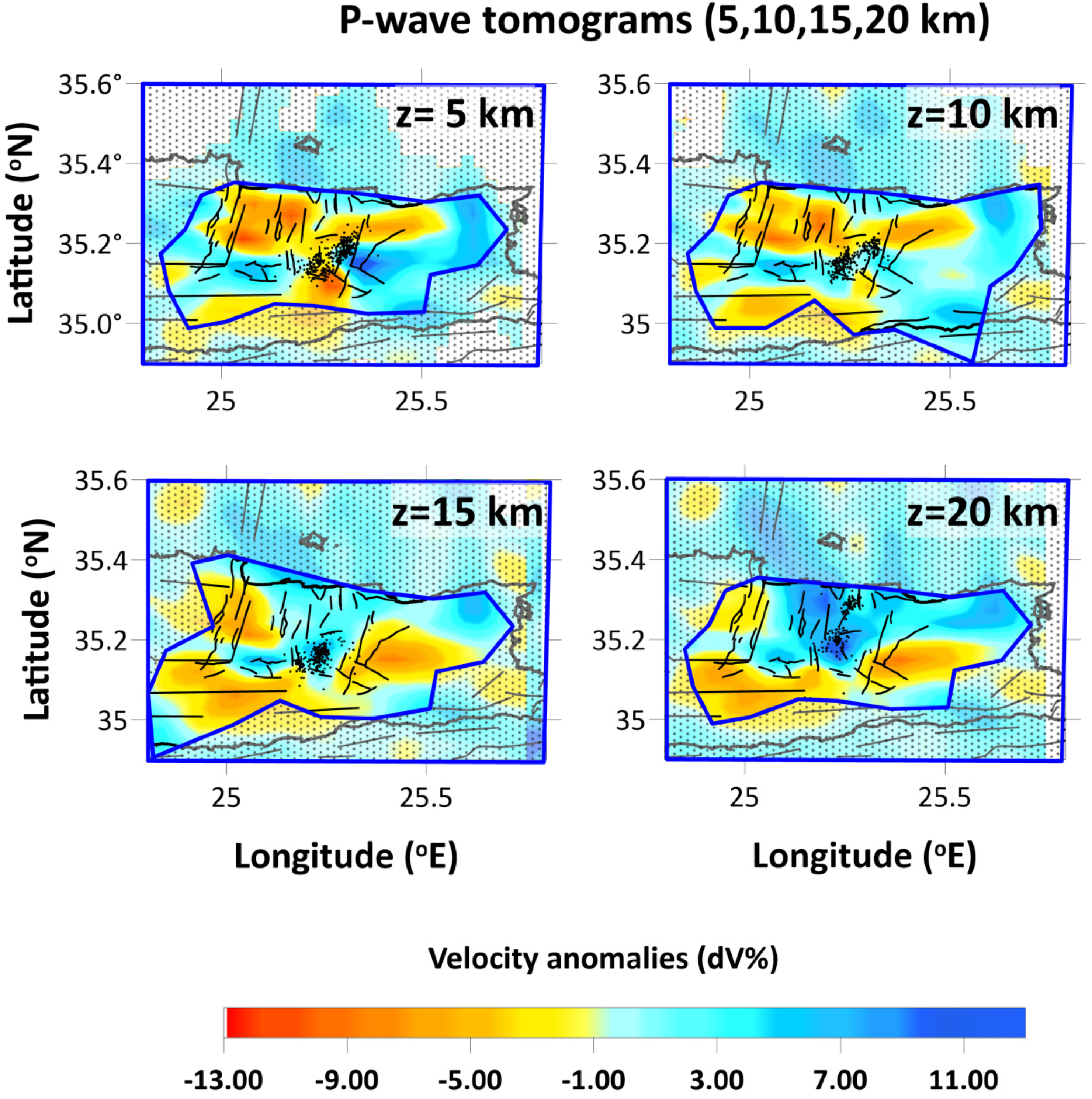
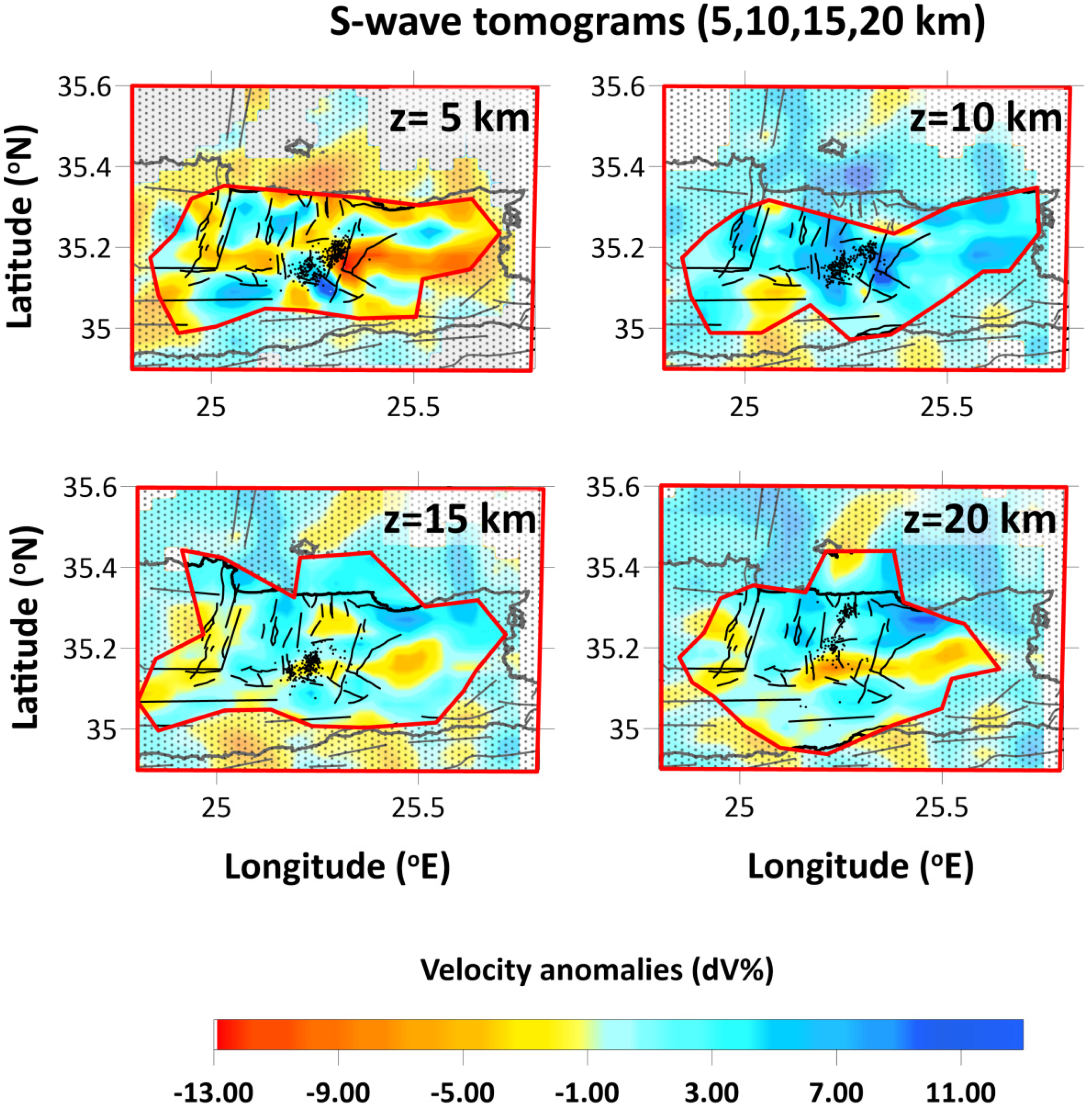
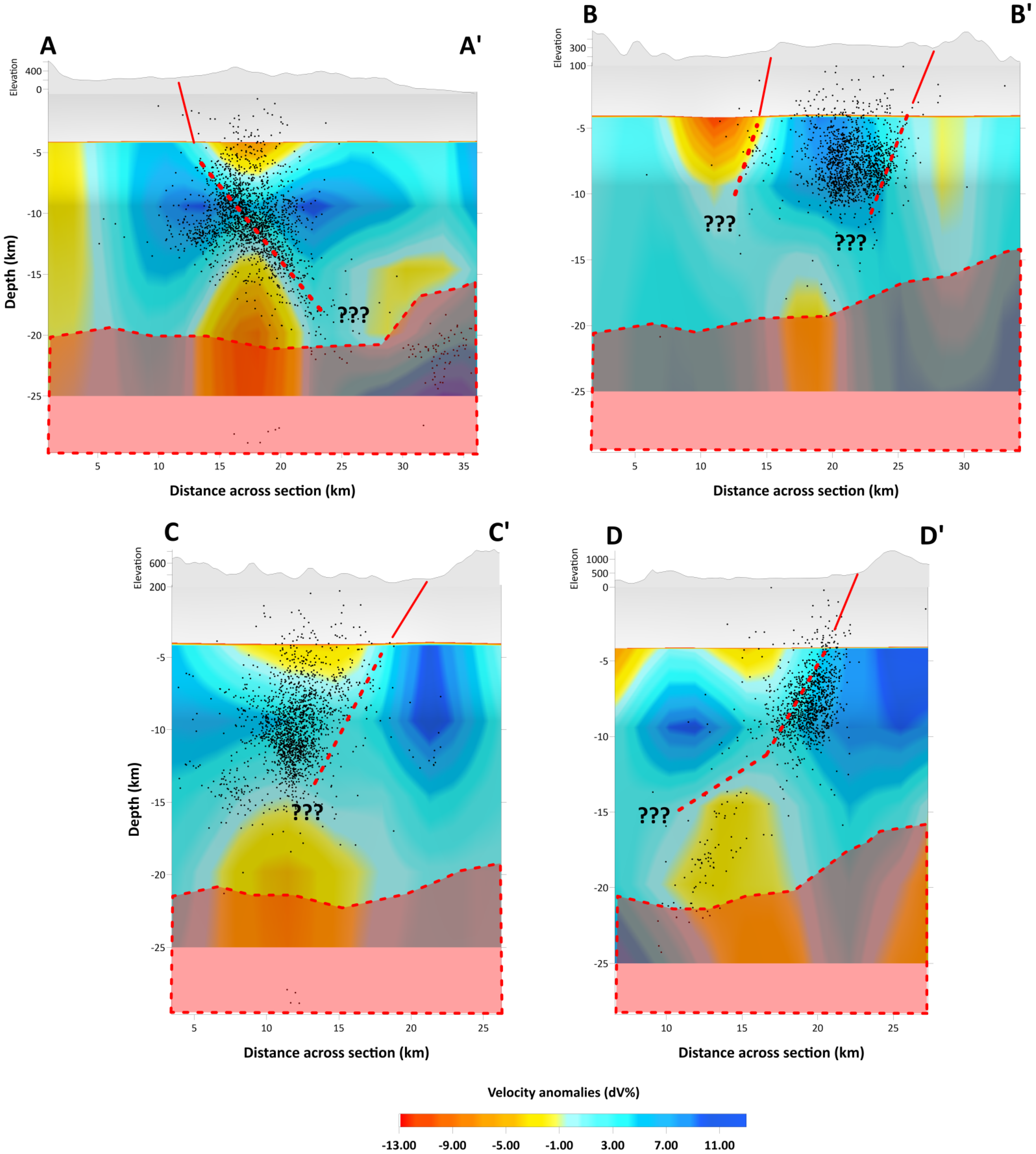
3. Travel Time Tomography

Local Earthquake Tomography (LET) techniques have been successfully applied to reveal the velocity structure in such cases of aftershock sequences. In this paper, the body-wave inversion was based on the LOcal TOmographic Software (LOTOS) by [33]. P- and S-phases of more than 800 earthquakes, recorded during the 2021–2022 time period by local and regional stations of the Hellenic Unified Seismological Network (HUSN) and the Hellenic Strong Motion Network (HSMN), located in Southern Greece, were used for the tomographic inversion. Checkerboard tests were performed to set the input parameter values that produced better resolution and increased the fidelity area. Regarding the 3D tomographic inversion, a dataset consisting of 12,236 P- and 9820 S arrival times was chosen, with at least 12 phases per event (Supplementary Material Figure S2). LOTOS code provides two alternative options: inversion for V_P and Vs (V_P–V_S scheme) using P and S travel-time residuals (dt_P and dt_S) and inversion for V_P and V_P/V_S ratio (V_P–V_P/V_S scheme) using dt_P and differential residuals, dt_S–dt_P. In this work, inversion was performed for V_P–V_S and V_P–V_P/V_S schemes, in order to obtain additional constraints concerning the V_P and Vs anomalies [33,34].

The stations’ coordinates, their elevation, and the body-wave arrival times are essential as input data to the algorithm. The hypocenter locations and the origin times are not necessarily needed, given that their determination is performed during the execution of the calculations. However, if preliminary hypocentral locations are available, they are used to decrease the processing time. Moreover, the available initial 1D velocity model [29] and a set of input parameters, i.e., parameterization, grid dimensions, and damping parameters, are defined by the user [33]. A nodal representation was employed, given that the velocity field, reconstructed by a three-dimensional grid, does not assume a specific geometry of heterogeneities [35]. The grid spacing (~2 km) was kept considerably smaller than the expected resolution length, to reduce the bias of the resulting models due to the grid configuration. The optimal grid mesh has been determined considering the stations/events geometry. In addition, to further decrease the influence of the model parameterization on the solutions, the inversion was repeated using four grid orientations (0°, 22°, 45°, and 67°). The inversion results, obtained for the previously mentioned grids, were stacked into one summary model, reducing the artifacts related to grid orientation, as described by [33].

The values of the P- and S-wave residuals during different iteration steps of the inversion procedure are presented in

Table 2. Average absolute values of P- and S-wave residuals and their cumulative reduction percentage during the inversion of experimental data.

Iteration	P-Residual (s)	P-residual Reduction (%)	S-Residual (s)	S-Residual Reduction (%)
1	0.269	0.00	0.437	0.00
2	0.211	21.50	0.248	43.14
3	0.194	27.63	0.222	49.12
4	0.188	30.08	0.218	50.10
5	0.186	30.85	0.211	51.69

. For the P- and S-data, the reduction of the residual is ~10% and 13%, respectively. The resulting P- and S-wave velocity anomalies with respect to the starting 1D velocity model are shown in horizontal depth slices (Figure 5 and Figure 6). The interpretation of the obtained results is limited to the unmasked confidence regions, given that they are characterized by reasonable reconstruction of the checkerboard model. The mean computed P and S anomalies for the study area do not exceed ±13%.

Strong NW-SE and E-W oriented negative velocity anomalies predominate at both the upper and the lower crust of Central Crete. These are observed down to 15 km depth in the tomograms of Figure 6 and Figure 7. Deeper than 20 km the model lacks resolution and can only be considered indicative, hence it is not discussed. At the depth slice of 5 km, a NE-SW-trending zone of negative body-wave velocity perturbations appears near the epicentral region of the Mw = 6.0 Arkalochori earthquake (Figure 6 and Figure 7). This anomaly follows the mean distribution of Alluvial deposits and post-alpine sediments which are bounded by positive (~13%) body-wave velocity perturbations, possibly connected to the older post-alpine sediments of Viannos formation and the Mesozoic carbonate rocks to the east and south of Arkalochori basin, respectively [13,22,36,37]. In the area north of Arkalochori, an E-W-trending anticorrelated pattern of negative P- and positive S-wave velocity anomalies are observed at the depth range of 5–10 km (35.20° N–35.30° N, 25.25° E–25.40° E). This anomaly coincides with the eastward bending of Kastelli’s normal fault direction, from the area east of Arkalochori towards the town of Malia (35.20° N–35.27° N, 25.34° E–25.45° E). In the depth slice of 15 and 20 km, and almost NNE-SSW discontinuity of positive to the west and negative to the east V_P anomalies (Figure 6) are identified along the west-dipping Agnos normal fault. Furthermore, cross-sections B-B’ and C-C’ in both primary (P) and secondary (S) wave velocity anomalies (Figure 8 and Figure 9), reveal this west-dipping structure that may be related to Agnos high-angle (~60°) normal fault [13,21,22,23,36,37].

4. Co-Seismic Ground Deformation

To study the co-seismic ground deformation on the epicentral area of the 27 September 2021 event, we combined space and ground-based geodetic techniques. Radar satellite data were used to produce differential interferograms to spatially study the co-seismic deformation. Moreover, geodetic data from continuous Global Navigation Satellite System (GNSS) stations operating on the broad affected area provided point-wise accurate 3D displacement vectors.

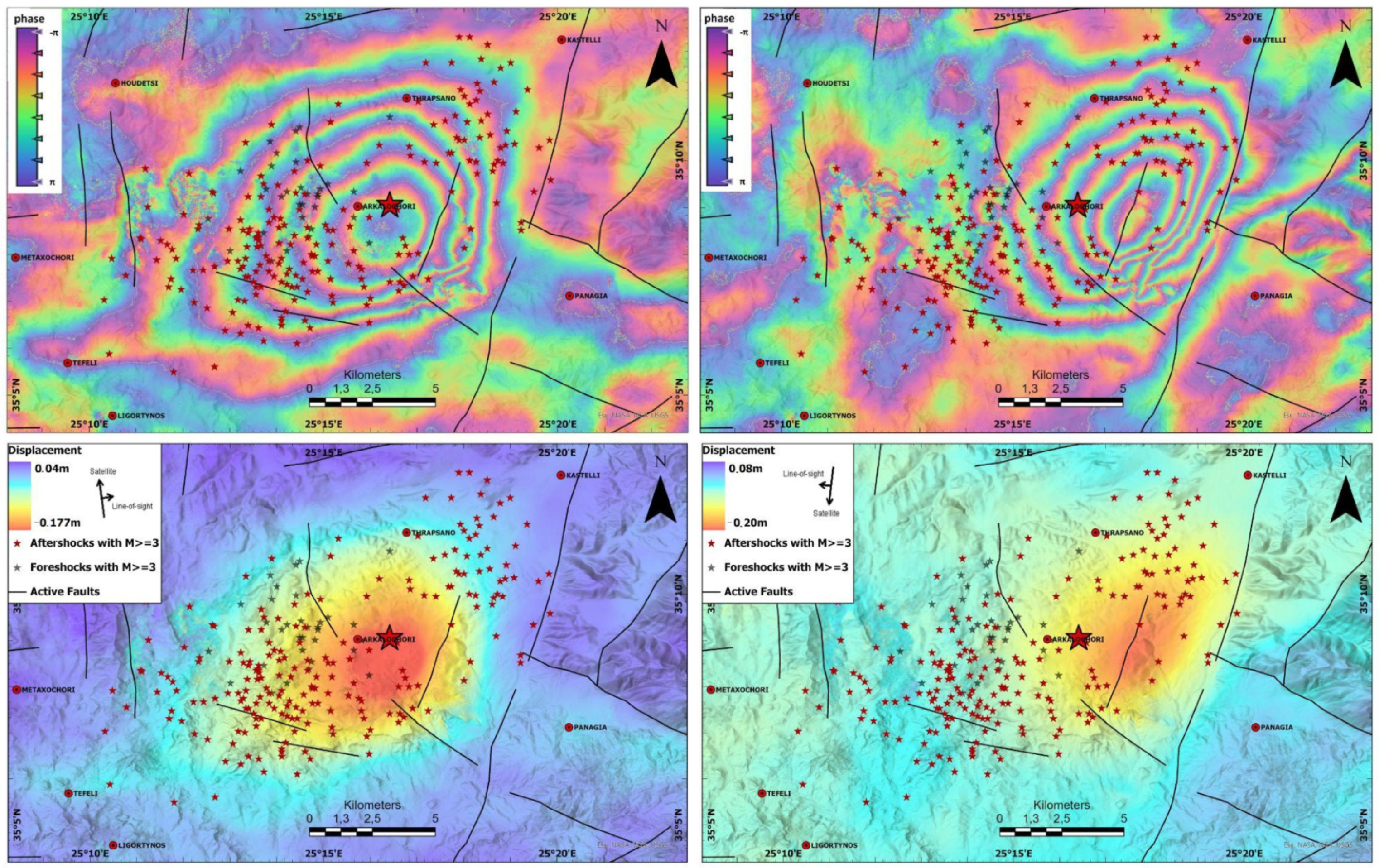
4.1. Interferometric Data and Results

The term SAR stands for Synthetic Aperture Radar [38]. Differential Interferometry (Differential InSAR technique-DInSAR) is an advanced technique [39] aimed at detecting surface movements due to geophysical phenomena or human interventions. Since the 1990s, the DInSAR technique has proven to be an interesting tool for measuring and observing ground deformation suitable for analyzing geodynamic processes, e.g., [40,41,42,43,44].

To map the co-seismic ground deformation due to the 27 September 2021 mainshock, we used two SAR image pairs, one on ascending and one on descending orbital geometries (

Table 3. The main characteristics of the SAR images used in this study.

Ascending Image Pair
Satellite	Ref./Repeat	Acquisition	Track	Orbit	Bperp (m)	Btemp (days)
S1B	Reference	23 September 2021	102	28,828	−111.36	6
S1A	Repeat	29 September 2021	102	39,899
Descending Image Pair
Satellite	Ref./Repeat	Acquisition	Track	Orbit	Bperp (m)	Btemp (Days)
S1A	Reference	25 September 2021	36	39,833	−28.08	6
S1B	Repeat	1 October 2021	36	28,937

), acquired from ESA’s Sentinel-1A and Sentinel-1B satellites (https://scihub.copernicus.eu/, accessed on 31 May 2022). In both cases, the reference image was the one before the earthquake occurrence, while the repeat image was the one that refers to the date after the event. Each reference–repeat pair was processed using the ESA’s SNAP software and two individual interferograms were generated. The topographic phase was subtracted using the SRTM 1 arc-second Digital Terrain Model, a 30-m resolution Shuttle Radar Topography Mission Digital Elevation Model (USGS 1 ARC-second SRTM DEM, https://doi.org/10.5066/F7DF6PQS, accessed on 31 May 2022), while the signal to noise ratio was enhanced by applying the adaptive power spectrum filter of [45] with a coherence threshold of 0.4.

The two-phase wrapped interferograms were then used to estimate co-seismic ground deformation. To calculate the terrain displacement, an unwrapping process was performed, and the phase unit was transformed into distance units in the satellite line of sight (LoS) for each interferometric pair. Finally, decomposition of the ascending and descending LoS displacement vectors was performed to extract the vertical (up–down) and horizontal (east–west) ground deformation components.

The two wrapped interferograms are of good quality and contain the phase difference, between reference and repeat images, produced by the main seismic event and its aftershocks until the 29th of September. Due to the low temporal geometric baselines (six days), there are no areas of low coherence in the interferograms. Six fringes, forming a lobe, are evident both in ascending and descending wrapped phase interferograms (Figure 10, upper part). This asymmetrical displacement pattern is characteristic of normal-faulting earthquakes indicating that the subsidence is larger than the uplift. Each interference fringe is a phase change that corresponds to a motion of 2.8 cm in the satellite line of sight.

The LoS displacement map in the ascending geometry shows negative LoS displacement values up to 18 cm, after the Mw = 6.0 earthquake including the ground deformation caused by all the seismic events that occurred in the time interval from 23 September to 29 September, (Figure 10, lower part), while the LoS displacement map in the descending geometry shows negative LoS values up to 20 cm after the Mw = 6.0 earthquake, including all the aftershocks, occurred until the 1st of October. On the descending orbital geometry, the maximum value of ground deformation has shifted east of the epicenter of the main earthquake (Figure 10) with respect to the ascending displacement map. After the decomposition of ascending and descending LoS displacement maps, the ground deformation in vertical (up–down) and east–west directions were extracted (Figure 11a). Subsidence up to 18 cm has been calculated from the displacement decomposition in the vertical (up–down) direction while no uplift was detected. The horizontal (east-west) displacement map reveals an eastward motion up to 6 cm in the area west of the epicenter and a westward movement up to 7.6 cm for the area east of Arckalochori (Figure 11b). The latter is in satisfactory agreement with [21] where the displacement is associated with the horizontal motion of the strike-slip component of the mean event focal mechanism.

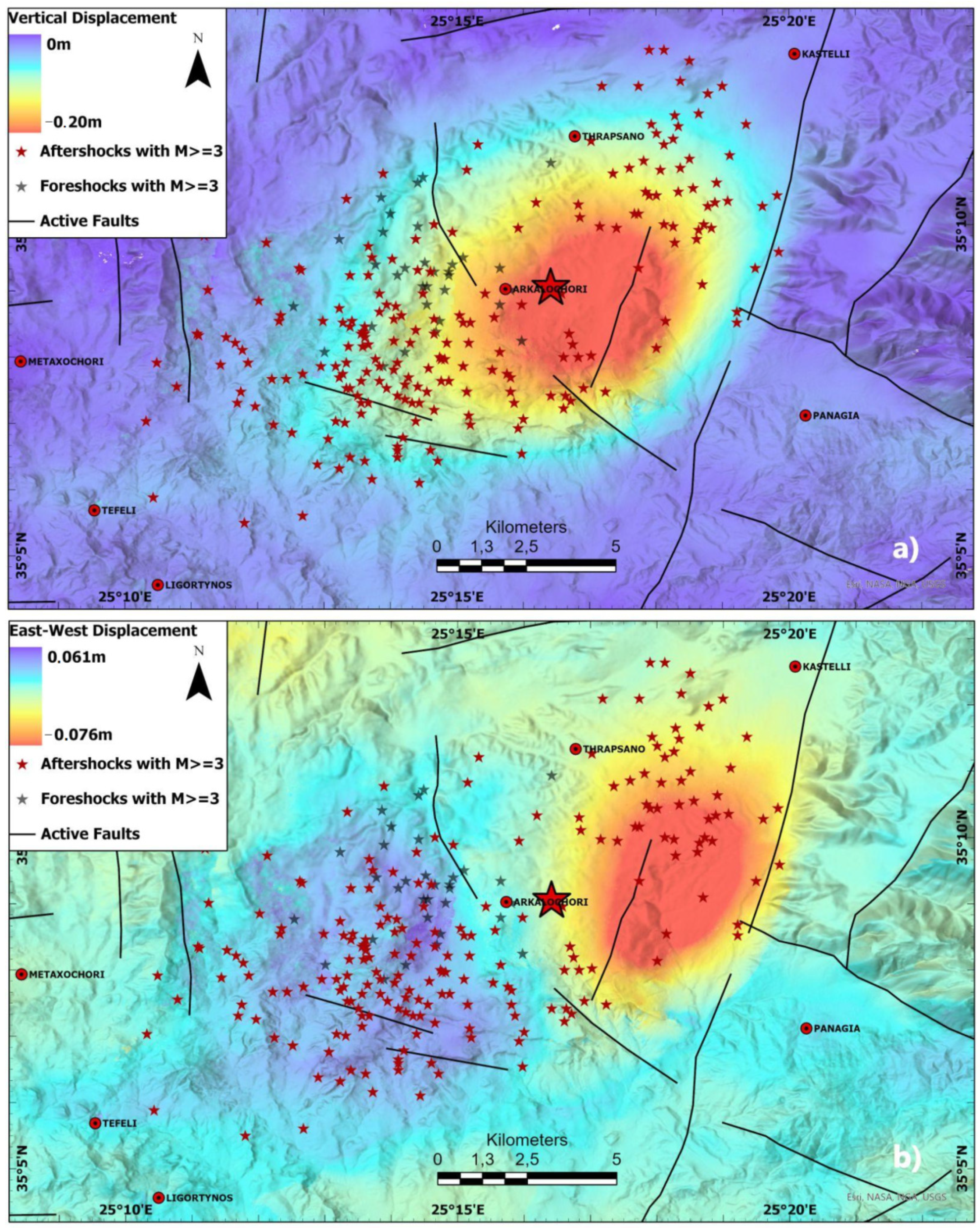
4.2. GNSS Data and Results

GNSS data from four continuous stations (belonging to the private network of METRICA SA) on the central-eastern part of Crete were used in the current study to measure the co-seismic displacement. One of the stations (ARKL) is located almost above the hypocenter of the main event, in Arkalochori. The other sites are located in the city of Heraclion (HERA station; ~24 km NNW of Arkalochori), in the village of Moires (MOI1 station; ~38 km WSW from epicenter), and in the Ierapetra region (IERA station; ~49 km ESE from the epicenter). Daily raw GNSS data from these four stations were processed for a period of several years before the 2021 seismic sequence up to 30 April 2022, using the Bernese v5.2 GNSS software [46].

In the processing procedure of the local GNSS data, several stations of the EUREF and IGS were included together with other auxiliary files. The absolute antenna phase center corrections were used, together with precise orbital solutions from the Center for Orbit Determination in Europe (CODE) and the Vienna Mapping Functions for the tropospheric modeling. For the coordinate estimation on static mode solutions, the precise double difference method was used. For ambiguity resolution, numerous strategies were applied, based on the length of the formed baselines between the GNSS stations. The processing resulted in the estimation of high-precision station coordinates. Time series were formed, annual velocities prior to the 2021 seismic event were calculated and co-seismic displacements were determined. The daily coordinates of the GNSS stations were estimated on the global ITRF2014 reference frame.

Based on the formed time series of the stations’ coordinates (Figures S5 and S6), for the pre-seismic period, all the stations show SE horizontal linear type of motion (with respect to ITRF 2014) and subsiding vertical motion, consistent with the velocity field of the area [47]. Calculating the change in the baseline distance between the stations prior to the seismic sequence it is observed that a small extension pattern occurred in the area, since lengthening on the baselines was recorded of small amplitude (~1.5 mm/year).

The main seismic event on Arkarochori caused, as is expected, strong ground displacement in the epicentral station ARKL as well as in the HERA station (

Table 4. GNSS stations’ coordinates and the respective vector of the co-seismic displacement.

Site	Latitude (°)	Longitude (°)	DEast (cm)	DNorth (cm)	DUp (cm)
ARKL	35.1339	25.2689	4.51 ± 0.11	7.85 ± 0.14	−15.45 ± 0.60
HERA	35.4241	25.1415	−0.54 ± 0.09	0.62 ± 0.19	0.57 ± 0.39

). The vector of the co-seismic displacement was calculated as the static shift of the station coordinates nine days prior to and three days after the 27 September 2021 event, to minimize the effect of possible post-seismic motions. The higher displacement was recorded on the ARKL station, while noticeable displacement occurred in the HERA site (Figure S5). The two other sites (MOI1 and IERA) have not shown any considerable co-seismic motion (Figure S6).

The displacement vector on ARKL site shows a strong subsiding component of ~16 cm and significant eastward and northward horizontal motion. Both the E–W and the vertical components deduced by the GNSS analysis agree with the interferometric results. Small discrepancies in the amplitude of the components deduced by the two techniques may be attributed to the incompetence of the DInSAR to define the north motional component that is inherent in the LoS vector, and in our case is quite noticeable (~8 cm). The displacement vector on HERA station shows NW horizontal co-seismic motion and a noticeable upward vertical component.

The overall image of the ground deformation in the epicentral area, based on both interferometric and GNSS results, defines a strong subsiding pattern with substantial horizontal motional component compatible with normal faulting activated structure.

In the period following the mainshock and up to 30 April 2022, the two GNSS sites in Arkalochori and Heraklion city show increased velocity values, compared to the previous period, indicating that the post-seismic relaxation is continuous up to this date.

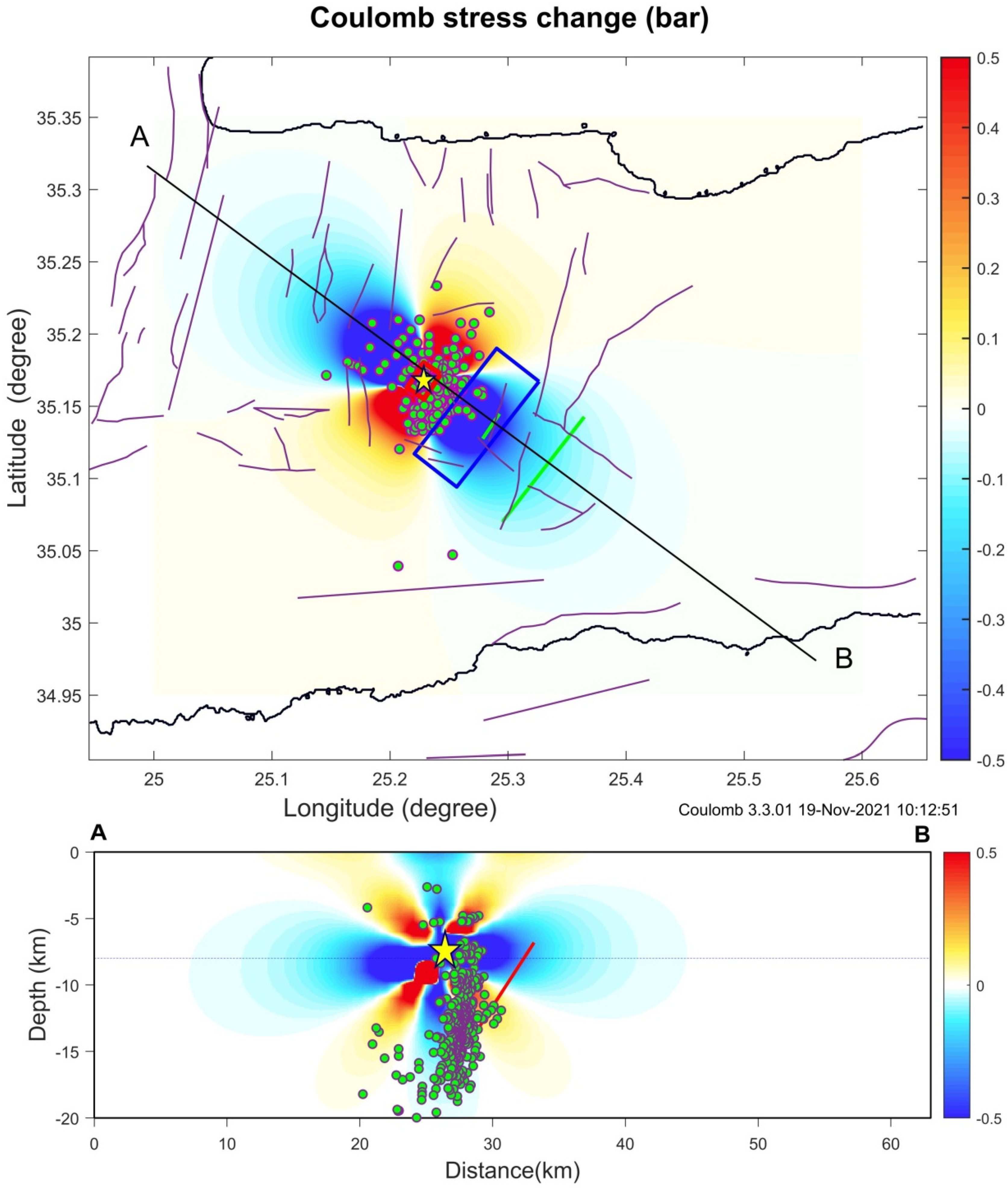
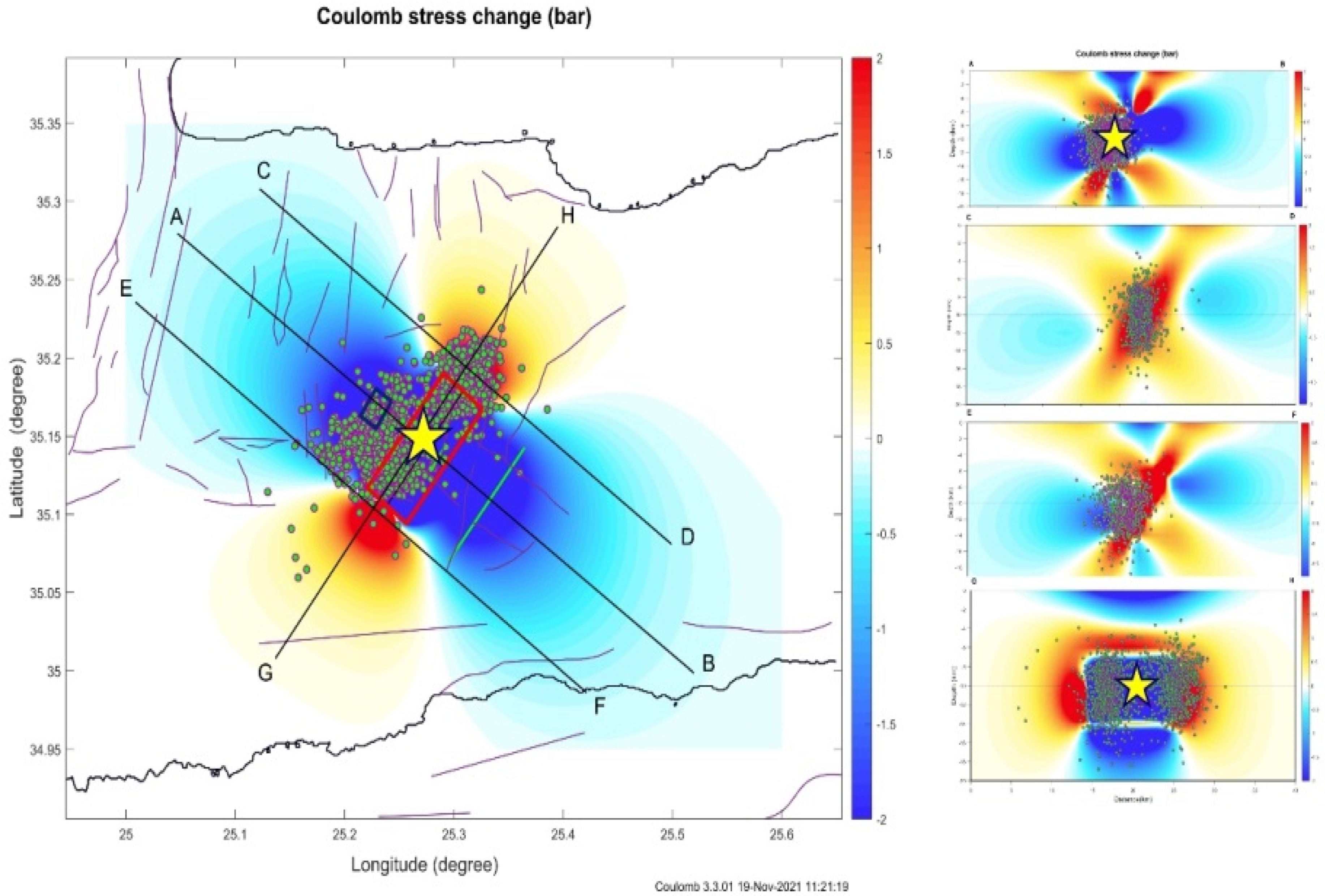
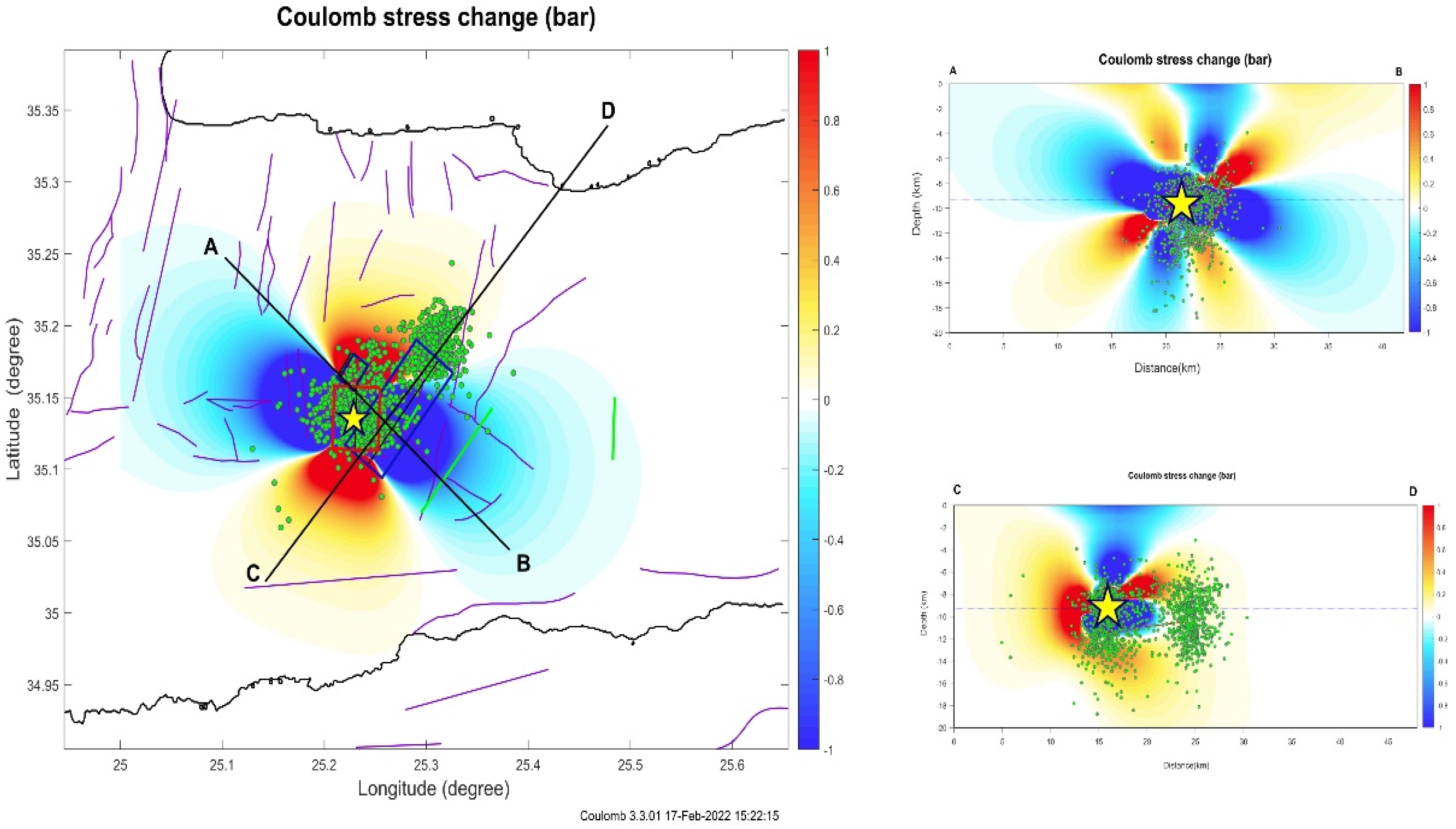
5. Spatial Footprint of Coulomb Stress Changes

Numerous studies of strong earthquakes show a correlation between the positive lobe of Coulomb stress changes and the locations of the majority of the most significant aftershocks, (e.g., [48,49]). A moderate earthquake of magnitude Mw = 4.9 occurred on 24 July 2021, 02:07:37 (UTC) accompanied by many aftershocks, before the main and catastrophic earthquake of magnitude Mw = 6.0 and its major aftershock of magnitude Mw = 5.3, which took place on 27 September 2021, 06:17:21 (UTC) and 28 September 2021, 04:48:08 (UTC), respectively. Herein, we examine the co-seismic static stress changes with respect to the aftershock spatial distribution during the event of Mw = 4.9, the Mw = 6.0 main event as well as the Mw = 5.3 major aftershock. The ΔCFS changes were determined via Coulomb3.3 software [50] in an elastic half-space and a uniform slip on the rupture planar surfaces.

The Coulomb Failure Stress changes (ΔCFS) are given by the Equation (3):

ΔCFS = Δτ − μ_f Δσ

(3)

where Δτ and Δσ are the in-shear stress and normal stress, respectively, while the μ_f is the effective friction coefficient [51,52,53]. For the shear modulus and Poisson’s ratio, we used the values of 3.3 MPa and 0.25, respectively, and a mean value for the coefficient of friction equal to μ_f = 0.4 [54].

To calculate the subsurface fault’s width and length, we used the empirical relations of [55] for each modeled earthquake. In addition, we used the available focal mechanism solutions from various agencies, and we present our preferred models for this study in

Table 5. Focal parameters of Mw = 4.9, Mw = 6.0 and Mw = 5.4 events.

Date	Hour	Minute	Lat.	Long.	Depth (km)	Mw	Strike	Dip	Rake	Agency	Length	Width	Mo (Nm)
24 July 2021	2	7	35.1676	25.2286	8	4.9	214	52	−95	NOA	2.3	2.56	9.116 × 1015
27 September 2021	6	17	35.1421	25.2734	10	6.0	218	57	−85	GFZ	7.61	10.3	1.1 × 1018
28 September 2021	4	48	35.1356	25.2312	9	5.3	182	22	−95	UOA	4.41	4.88	1.30 × 1017

.

Figure 12 shows the determined co-seismic ΔCFS changes caused by the event of magnitude Mw = 4.9 at a centroid depth of 8.0 km and the vertical cross-sections AB and CD. The spatial distribution of the ΔCFS reveals a stress decrease towards NW and SE and a stress increase towards NE and SW of the ruptured fault. The aftershocks during this period and before the main event of Mw = 6.0 are distributed mainly along and under the fault up to 20 km depth. The ΔCFS values at the hypocenters of the Mw = 6.0 and Mw = 5.4 events were calculated, and the results provide −0.104 MPa and +0.0169 Mpa, respectively. The co-seismic Coulomb stress variations caused by the strong earthquake of Mw = 6.0 and its major aftershock (Mw = 5.4) at centroid depths of 10.0 km and 9.0 km, respectively, as well as the spatial distribution of aftershocks, are presented in Figure 13 and Figure 14. For both seismic events, the same pattern on the spatial distribution of the ΔCFS is observed, which indicates a stress decrease towards NW and SE and a stress increase towards NE and SW of the ruptured faults.

The focal mechanism of the mainshock was related to normal faulting and only a small portion of the strike-slip component was involved. A similar solution is evident for the largest foreshock (Mw4.9) and aftershock (Mw5.3) (Table 5) although, in the latter, the strike-slip component is increased.

From the obtained co-seismic ΔCFS changes we thus observe that most aftershocks, including those of greater magnitude, occurred within positive static stress changes produced by the major earthquake, and by the strongest aftershock. This suggests that the spatial distribution of aftershocks, including the significant ones, are controlled by the co-seismic Coulomb stress changes produced during the Mw = 6.0 mainshock and the major events of the sequence.

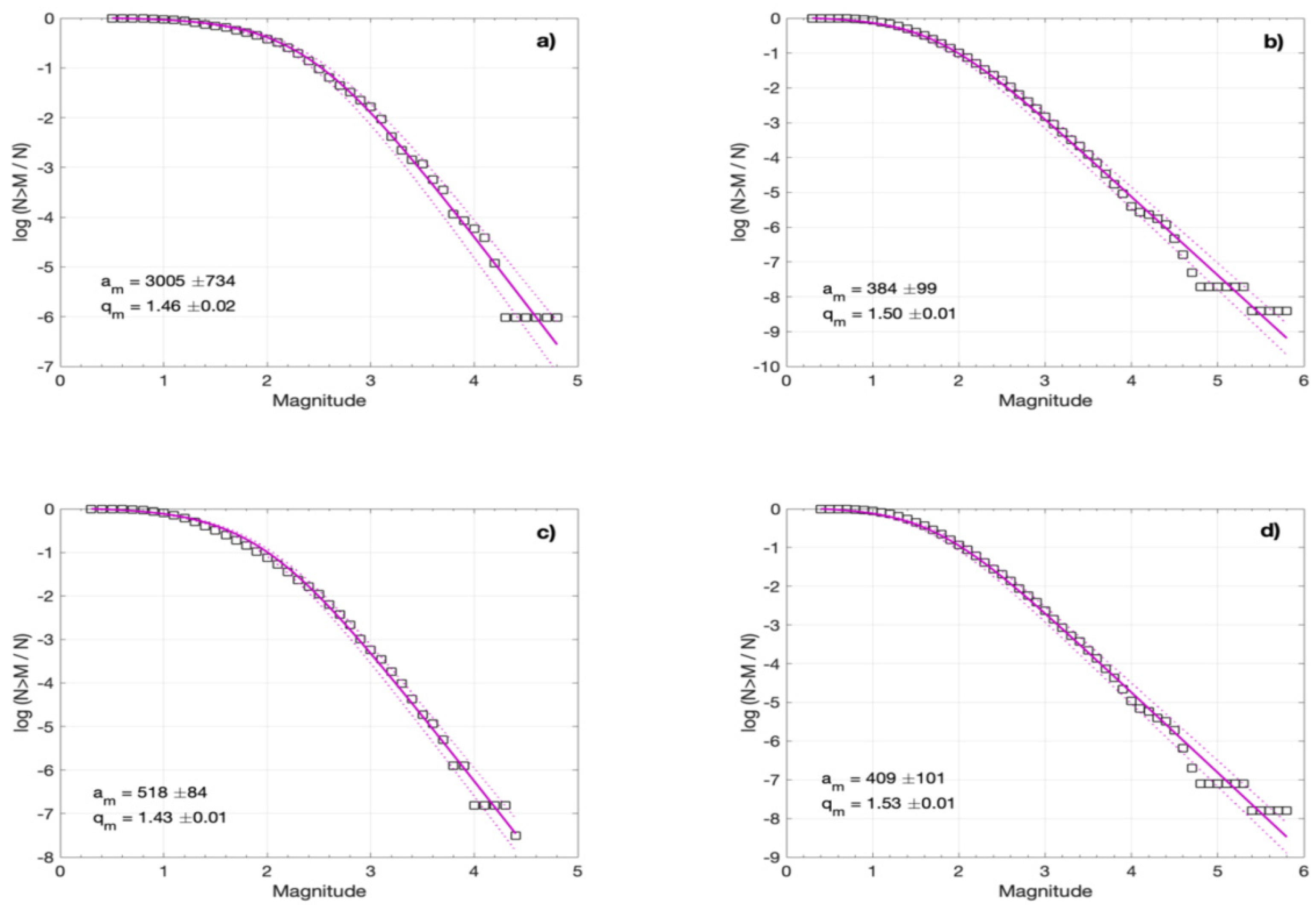
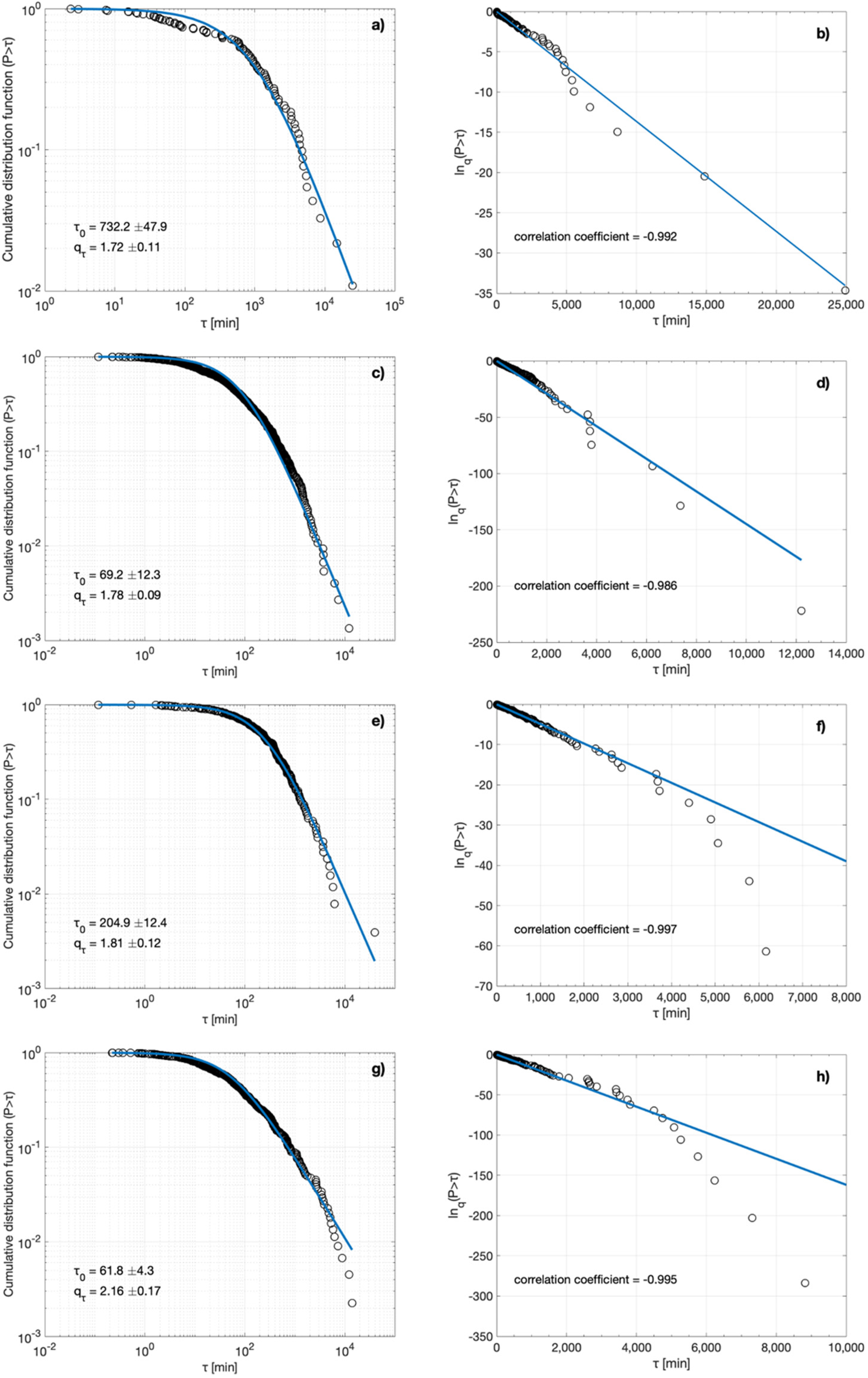
6. Frequency-Magnitude Scaling Properties of the Foreshock and Aftershock Sequences in Terms of Non-Extensive Statistical Physics

The frequency–magnitude distribution (FMD), known as G-R law [56], is of vital importance for the characterization of a seismic sequence [56,57,58,59,60,61,62,63,64,65,66,67,68,69] and is expressed by Equation (4):

$$logN=a-bM$$

(4)

where N is either the discrete frequency of magnitudes M in each magnitude bin, or the cumulative frequency of magnitudes ≥M; α, b are parameters determined by the earthquake catalog data, and the slope b of the G-R law expresses the relative number of the small magnitude earthquakes to the large magnitude ones and α is a measure of the seismicity level. In terms of geophysics, the b-value is considered as a possible stress meter, e.g., [58]. In this context, low b indicates high material heterogeneity and concentrated stress while high b implies asymmetrically distributed stress. For details on the b-values for the Arcalochori seismic sequence see [21].

An alternative model that describes the frequency–size distribution of earthquakes from the first principles of non-extensive statistical physics (NESP) was introduced in [70]. This model is based on Tsallis Entropy, a generalization of the Boltzmann–Gibbs one [71] that offers a coherent theoretical framework for analyzing complex dynamical systems with fractal features and long-range correlations [72]. The approach introduced in [70] considers that the seismic energy E is related to the size of the fragments that fill the space between the activated fault blocks. Then, by considering that the earthquake magnitude is related to the radiated seismic energy as $M=\frac{2}{3}logE$, the cumulative distribution function N(>M) of earthquake magnitudes M can be deduced as [73]:

$$\frac{N\left(>M\right)}{N}={\left[1-\left(\frac{1-q_m}{2-q_m}\right)\left(\frac{{10}^M}{{\alpha }_m^{\raisebox{1ex}{$2$}\!\left/ \!\raisebox{-1ex}{$3$}\right.}}\right)\right]}^{\frac{2-q_m}{1-q_m}}$$

(5)

where q_m is the entropic index and α_m a model parameter that expresses the proportionality between the seismic energy and the size of the fragments. In [74] updated the derived equation to include the minimum earthquake magnitude M₀ in a seismic catalog, which now reads as:

$$\frac{N\left(>M\right)}{N}={\left[\frac{1-\left(\frac{1-q_m}{2-q_m}\right)\left(\frac{{10}^M}{{\alpha }_m^{\raisebox{1ex}{$2$}\!\left/ \!\raisebox{-1ex}{$3$}\right.}}\right)}{1-\left(\frac{1-q_m}{2-q_m}\right)\left(\frac{{10}^{M_0}}{{\alpha }_m^{\raisebox{1ex}{$2$}\!\left/ \!\raisebox{-1ex}{$3$}\right.}}\right)}\right]}^{\frac{2-q_m}{1-q_m}}$$

(6)

The derived model, in the form of Equation (6), has extensively been used to describe the earthquake dynamics of local and regional seismicity, (e.g., [75,76,77,78,79,80,81,82,83,84,85,86]). In comparison to the Gutenberg–Richter (G-R) scaling law, the FA model provides a reasonable explanation of recorded earthquake magnitudes over a wider range of scales, while the b-value may be obtained as a special case for values over a certain threshold magnitude [75.86] as:

$$b=\frac{\left(2-q_E\right)}{\left(q_E-1\right)}$$

The result of the application of the NESP model (Equation (6)) to the observed cumulative distributions N(>M) of earthquake magnitudes for the foreshock and aftershock sequences of the Mw = 6.0 mainshock, as well as for the NE and SW spatial clusters, are shown in Figure 15. The model provides a good fit to the observed distributions over the entire range of magnitudes, for the model parameters referred to in

Table 6. Parameter values for the foreshock and aftershock sequences in Arkalochori, as well as for the NE and SW aftershock clusters. N is the number of events (with M ≥ M_c), Mc the magnitude of completeness, a_m, q_m the parameters of the NESP model (Equation (6)) and τ₀, q_τ the parameters of the q-exponential function for the inter-event time distribution (Equation (10)).

	N	Mc	αm	qm	τ0	qτ
Foreshocks	410	2.8	3005 ± 734	1.46 ± 0.02	732.2 ± 47.9	1.72 ± 0.11
Aftershocks (both NE and SW clusters)	4465	2.5	384 ± 99	1.50 ± 0.01	69.2 ± 12.3	1.78 ± 0.09
NE cluster	1815	2.5	518 ± 84	1.43 ± 0.01	204.9 ± 12.4	1.81 ± 0.12
SW cluster	2431	2.5	409 ± 101	1.53 ± 0.01	61.8 ± 4.3	2.16 ± 0.17

and Figure 15. The greater q_m value for the SW cluster indicates greater tectonic instability in this region where the mainshock and the major aftershocks occurred.

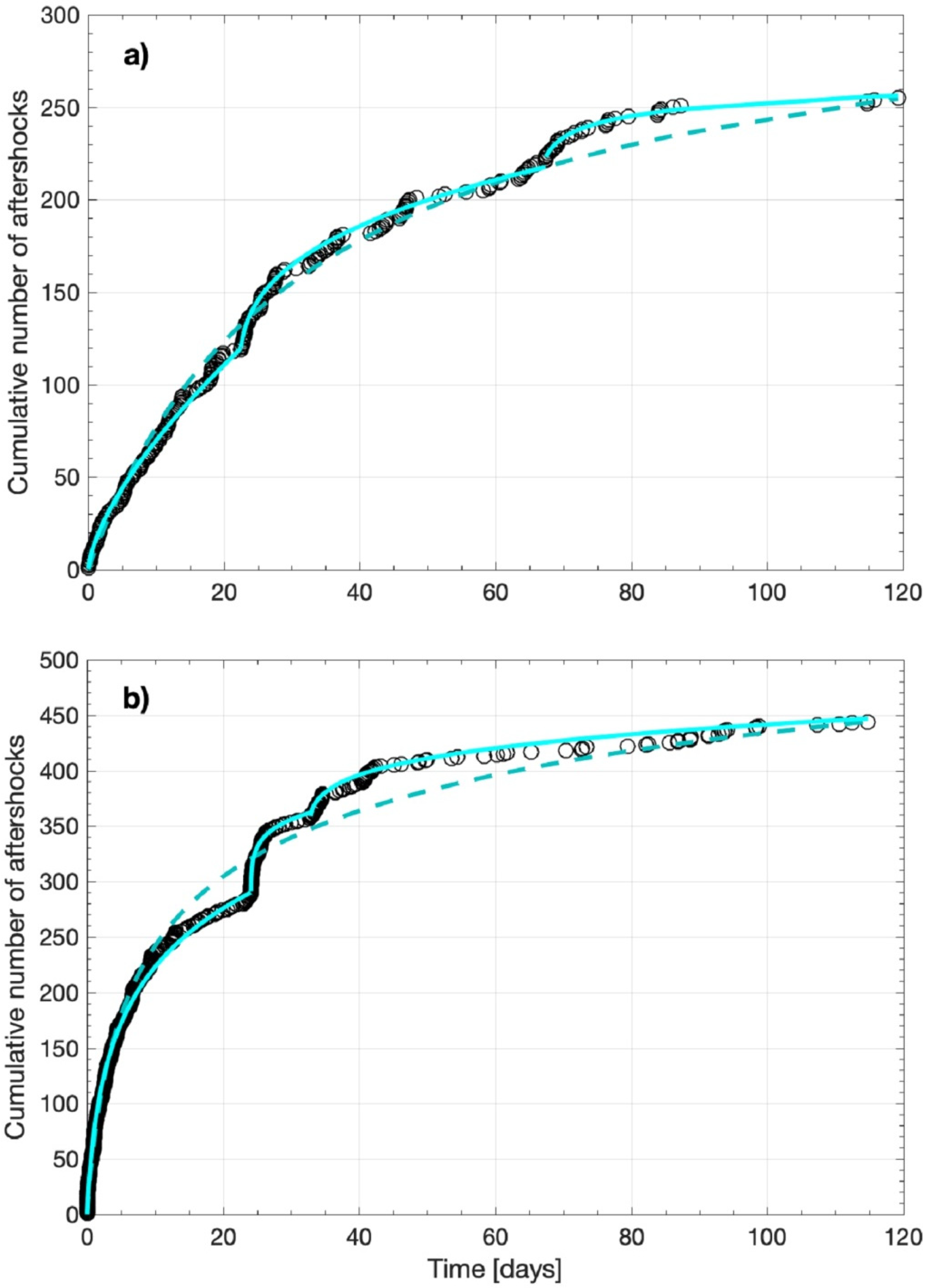
7. Temporal Properties of the Aftershock Sequence

7.1. Aftershock Production Rate and Modelling

It has long been recognized that the number of aftershocks following a major event resembles a power law decay with the time that expresses the relaxation process after the mainshock. This mathematical relationship takes the form of the so-called modified Omori’s scaling law [87,88]:

$$n\left(t\right)=K{\left(t+c\right)}^{-p}$$

(7)

where n(t) is the production rate of aftershocks $n\left(t\right)=dN\left(t\right)/dt$, N(t) is the number of aftershocks in time t after the mainshock, K and c are constants and p the power law exponent that usually takes values in the range 0.9 < p < 1.6 [89]. Moreover, the cumulative frequency of aftershocks N(t) is estimated from n(t) as:

$$N\left(t\right)=\underset{0}{\overset{t}{{\displaystyle \int }}}n\left(s\right)ds=\{\begin{array}{c}K\left[c^{1-p}-{\left(t+c\right)}^{1-p}\right]/\left(p-1\right),\mathrm{for} p\ne 1\\ Kln\left(t/c+1\right),\mathrm{for} p=1\end{array}$$

(8)

Herein, we use the previous equation to model the evolution of the aftershocks in terms of the cumulative frequency of aftershock activity that followed the Mw6.0 mainshock. We focus on the two major aftershocks clusters, the NE and SW spatial clusters that were discussed previously, and apply the maximum likelihood method to estimate the model parameters of Equation (8) [90]. In Figure 16 the cumulative number of aftershocks (for M ≥ M_c) with time is shown for the two spatial clusters along with the modified Omori’s law (Equation (8)), which generally provides a fair fit for the parameter values given in

Table 7. The considered mainshock, the duration (in days), the number of events (N), and the MLE of the modified Omori formula parameters for the NE and SW aftershock clusters, along with their associated uncertainties. AIC is the estimated Akaike Information Criterion for each model.

Cluster	Model	Mainshock	Duration (Days)	N	K	c (Days)	p	AIC
NE cluster	Single model	M5.8 27/09/21	119.3	256	71.02 ± 14.45	28.35 ± 0.57	1.85 ± 0.08	–72.4
	Composite model	M5.8 27/09/21	22.8	120	10.57 ± 7.18	0.01 ± 1.63	0.35 ± 0.12	–125.7
		M4.3 20/10/21	44.6	92	10.95 ± 3.98	0.24 ± 0.65	0.66 ± 0.06
		M3.7 03/12/21	51.9	44	11.57 ± 8.56	1.50 ± 1.63	1.10 ± 0.28
SW cluster	Single model	M5.8 27/09/21	114.8	446	165.65 ± 126.80	1.76 ± 1.33	1.18 ± 0.16	–1130
	Composite model	M5.8 27/09/21	24.1	290	81.09 ± 35.98	0.67 ± 1.15	1.01 ± 0.36	–1304
		M4.5 21/10/21	8.7	68	12.00 ± 4.66	0.01 ± 0.11	0.86 ± 0.19
		M3.7 03/12/21	82.0	88	10.00 ± 4.55	0.26 ± 0.32	0.77 ± 0.08

. However, large aftershocks may trigger secondary aftershock sequences embedded in the aftershock sequence of the mainshock. In this case, several Omori regimes may be used to model the aftershocks production rate n(t) [89,90,91]:

$$n\left(t\right)=K_1{\left(t+c_1\right)}^{-p_1}+H\left(t-t_2\right)K_2{\left(t-t_2+c_2\right)}^{-p_2}+H\left(t-t_3\right)K_3{\left(t-t_3+c_3\right)}^{-p_3}$$

(9)

where H(·) denotes a unit step function and t₂, t₃ indicates the occurrence times of secondary aftershock sequences. In Figure 16, breaks are observed in the cumulative number of aftershocks for both spatial clusters that are associated with strong aftershocks and the generation of secondary aftershock sequences. Hence, we investigate if the composite model of Equation (9) fits better the observed distribution. By setting t₂ = 22.8 days and t₃ = 67.4 days that designate the occurrence times of strong aftershocks following the mainshock for the NE cluster (Table 7), we find that the composite model provides a better fit to the observed distribution (Figure 16), which is further confirmed by the smaller Akaike Information Criterion (AIC) value in comparison to the single Omori regime (Table 7).

A similar result is obtained for the SW cluster. In this case, we used t₂ = 24.1 days and t₃ = 32.8 days which mark the occurrence times of strong aftershocks in the SW cluster (Table 7). The composite model provides a better fit to the observed distribution, in comparison to the single Omori regime, for the parameter values given in Table 7.

7.2. The Interevent Times Distributions for the Foreshock and Aftershock Sequences

Furthermore, we study the temporal scaling properties of the foreshock and aftershock sequences by investigating the interevent times (or waiting times) distributions between the successive events. In this analysis, earthquakes are considered as a point process in time, marked by the magnitude of the event, with interevent times τ between the successive events defined as τ_i = t_i+1 − t_i, where t_i is the time of occurrence of the ith event {i = 1, 2, …, N − 1} and N the total number of events. First, we construct the cumulative distribution of the interevent times (M ≥ M_c) for the foreshock and aftershock sequences, as well as for the NE and SW spatial clusters. We then model the observed distributions with the q-exponential function, derived in the framework of NESP [72,82,84,86,92,93,94,95,96]. It has been shown in various studies that the q-exponential function appropriately describes the distribution of interevent times in global, regional, and volcanic earthquake activity, as well as in aftershock sequences [73,74,75,76,77,78,79,80,81,82,83,84,85,86,91,92,93,94,95,96].

If P(>τ) = Ν(>τ)/Ν₀ is the cumulative distribution function (CDF) of the interevent times, with N(>τ) the number of interevent times with a value greater than τ and Ν₀ their total number, then the q-exponential cumulative distribution is given by [92]:

$$P\left(>\tau \right)={\exp }_q\left(-\frac{\tau }{{\tau }_0}\right)$$

(10)

where τ₀ is a constant in time units and exp_q(x) is the q-exponential function defined as:

$${\exp }_q\left(x\right)={\left[1+\left(1-q\right)x\right]}^{\raisebox{1ex}{$1$}\!\left/ \!\raisebox{-1ex}{$\left(1-q\right)$}\right.},$$

(11)

when 1 + (1 − q)x ≥ 0 and exp_q(x) = 0 in all the other cases. Its inverse is the q-logarithmic function: ${\ln }_q\left(x\right)=\frac{1}{1-q}\left(x^{1-q}-1\right)$. In the limit of q → 1, the q-exponential and q-logarithmic functions lead to the ordinary exponential and logarithmic functions, respectively.

In Figure 17, we present the cumulative distributions P(>τ) for the foreshock and aftershock sequences and for the two spatial clusters in log-log plots. In all four cases, the q-exponential cumulative distribution (Equation (10)) provides a good fit to the observed distributions for the parameter values given in Figure 17 and Table 6. This is further confirmed by the expected linear dependence of corresponding q-logarithmic distributions ln_qP(>τ) with τ [77], which are shown in the right panels of Figure 17. In all cases, the q-logarithmic function describes the observed distributions with high correlation coefficients, shown in the corresponding panels. The high values of q_τ (Table 6) indicate long-range temporal correlations in the evolution of the earthquake activity and further confirm the high q_τ values observed in aftershock sequences [84,96,97,98].

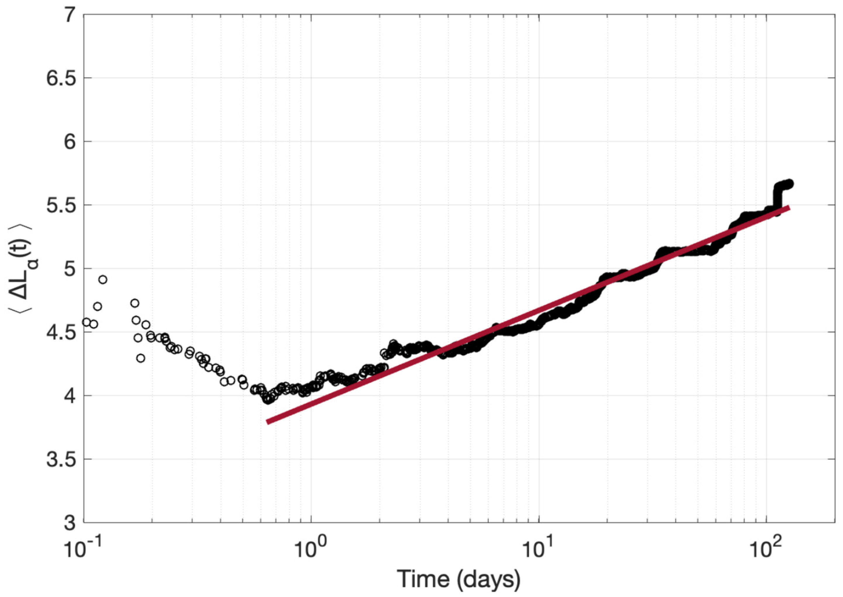
7.3. Scaling of the Aftershocks Focal Zone with Time

The growth of the aftershock focal zone with time can provide valuable information regarding the triggering mechanisms of earthquake migration. This migration pattern observed in many cases frequently scales as the logarithm of time [97,98,99,100,101,102]. Various studies, based on numerical simulations [103,104], as well as on real cases [97,105], suggest that this logarithmic migration pattern signifies that aftershocks migration is driven by afterslip. In this case, aftershocks are generated as the outcome of afterslip propagation along the activated fault. To anticipate the growth of the aftershock focal zone with time as the outcome of afterslip, ref. [106] have recently introduced a numerical model. In this model, asperities on a fault are stressed initially by regional creep occurring at a steady deformation rate during the inter-seismic period. As the mainshock occurs, some of the asperities slip co-seismically, transferring large positive Coulomb stresses to the surrounding creeping regions. During the post-seismic phase, the stress-loaded regions can accommodate large amounts of afterslip and when a critical level of afterslip is reached, aftershocks are triggered. Static stress changes in the model are thought to trigger aftershocks only during the early post-seismic phase so that most aftershocks are triggered by afterslip. In this case, the seismicity rate R(t) can then be proportional to the afterslip rate V(t) [103,106,107]:

$$V\left(t\right)=\frac{V_{+}exp\left(\raisebox{1ex}{$t$}\!\left/ \!\raisebox{-1ex}{$t_r$}\right.\right)}{1+\left(\frac{V_{+}}{V_L}\right)\left[exp\left(\raisebox{1ex}{$t$}\!\left/ \!\raisebox{-1ex}{$t_r$}\right.\right)-1\right]}$$

(12)

where V₊ and V_L are the sliding velocity just after the end of co-seismic rupture and the long-term loading velocity after the mainshock and t_r the duration of the post-seismic phase. Considering the previous equation, the seismicity rate R(t) can then be given by:

$$R\left(t\right)=\frac{R_{+}exp\left(\raisebox{1ex}{$t$}\!\left/ \!\raisebox{-1ex}{$t_r$}\right.\right)}{1+\left(\frac{R_{+}}{R_L}\right)\left[exp\left(\raisebox{1ex}{$t$}\!\left/ \!\raisebox{-1ex}{$t_r$}\right.\right)-1\right]}$$

(13)

where R₊ and R_L are the seismicity rates just after the end of co-seismic rupture and the long-term one after the mainshock, respectively. If $\dot{\tau }$ is the stressing rate and ΔCFS the co-seismic Coulomb stress changes induced by the mainshock, then the parameters t_r and R₊ are given by $t_r=A\prime /\dot{\tau }$ and $R_{+}=R_{L}exp\left(\Delta CFS/A\prime \right)$, where $A^{\prime }=\left(a-b\right)\sigma$, with a and b the rate and state frictional parameters and σ the effective normal stress. For $t/t_r\ll 1$, Equation (13) yields a decay rate for R(t) proportional to $1/t$, which is consistent with a modified Omori decay rate with p = 1 [87].

With the previous assumptions, the distribution of afterslip velocities can be deduced. Initially, a fault with only depth varying normal stress, stressing rate, and rheological parameter A′ is considered. If the initial Coulomb stress field varies with the strike direction x, then aftershocks migrate along x, forming the initial distribution of afterslip velocities. Then, the propagation velocity V_p of the aftershocks focal zone, in the early stage of the post-seismic phase, which typically lasts several weeks or months after the mainshock, is given by [103]:

$$V_p=\frac{A^{\prime }}{t}\times {\left(-\frac{\partial \Delta CFS}{\partial x}\right)}^{-1}$$

(14)

The expansion of the aftershocks zone L_a between time t_i and t (t > t_i) is now given by:

$$\mathsf{\Delta }{L}_a\left(t\right)=L_a\left(t\right)-L_a\left(t_i\right)=A^{\prime }\times {\left(-\frac{\partial \mathsf{\Delta }CFS}{\partial x}\right)}^{-1}ln\left(\frac{t}{t_i}\right)$$

(15)

The latter equation manifests the logarithmic expansion of the aftershocks zone with time and for a smooth co-seismic Coulomb stress field, implies its slow migration.

Since the estimated co-seismic Coulomb stress field ΔCFS (Equation (3)) can be significantly different from the “real” one, ref. [103] suggested a mean Coulomb stress gradient to be used. In this case, Equation (15) becomes:

$$\langle \Delta L_a\left(t\right)\rangle =A^{\prime }\times \langle {\left(-\frac{\partial \Delta CFS}{\partial x}\right)}^{-1}\rangle ln\left(\frac{t}{t_i}\right)=\zeta A^{\prime }\frac{l_c}{\Delta \sigma }ln\left(\frac{t}{t_1}\right)$$

(16)

In the latter equation, l_c is the radius of the co-seismic rupture, Δσ the mean value of the mean co-seismic stress drops and ζ a constant. For an idealized Coulomb stress field, ζ takes the value of 2.77 [103].

In the light of the previously described model, we investigated the scaling properties of the aftershock focal zone with time for the Arkalochori aftershock sequence. In the analysis, we used the relocated catalog for the events with M ≥ M_c = 2.5 to estimate the mean distance of aftershocks from the mainshock $\langle \Delta L_a\left(t\right)\rangle$ with time t, along the horizontal dimensions. The result is shown in Figure 18, as a function of the logarithm with time. The expansion of the aftershocks zone becomes apparent, as $\langle \Delta L_a\left(t\right)\rangle$ grows systematically with time after the surpass of one day from the mainshock. This growth can well be described by the afterslip front (Equation (16)) for over a period of one hundred days (R² = 0.97). We note that the logarithmic time dependence starts almost after the first day from the main event, possibly suggesting that after that time the system starts to be driven by an afterslip process.

Furthermore, from Equation (16) the rheological parameter A′ can be determined once the slope s_a of the afterslip front is known. From Figure 18, we obtain s_a = 0.320 ± 0.003. Then, from Equation (16), $s_a=\frac{d\langle L_a\left(t\right)\rangle }{dlnt}=\zeta A^{\prime }\frac{l_c}{\Delta \sigma }$, where l_c is the radius of the co-seismic rupture and Δσ the co-seismic stress drop. For a simple model of circular rupture, l_c can approximately be determined as $l_c={\left(\frac{7}{2}\frac{M_o}{\Delta \sigma }\right)}^{1/3}$ [51]. Τhe average stress drop for normal fault earthquakes in Greece is Δσ = 5.5 ± 1.5 MPa [108,109], while the mainshock’s seismic moment is M_o = 1.1 × 10 ¹⁸ Nm (Table 4) [21,22,23]. Then, we estimate the value of l_c ≈ 8.9 km for the co-seismic rupture. For ζ = 2.77, the rheological parameter A′ takes the value of A′ ≈ 0.71 MPa, which is within the range 0.1–1 MPa of A′ values that are usually found [97,98,103]. This value is considerably higher than other A′ values that were estimated for recent normal fault mainshocks in Greece, as [97] estimated A′ ≈ 0.041 MPa for the 2020 Mw7.0 Samos earthquake, while [98] estimated the value of A′ ≈ 0.29 MPa for the 2021 Mw6.3 Northern Thessaly earthquake.

8. Concluding Remarks

The 2021 Arkalochori earthquake is a characteristic event in the time history of Central Crete. The main event of 27 September 2021 Mw6.0 was a reminder that strong earthquakes do occur onshore Crete. In the present work the patterns and the scaling properties of the 2021–2022 earthquake sequence that occurred at Central Crete, are presented.

A relocation procedure has managed to improve the relative locations of the foreshock epicenters, which are concentrated in the vicinity of the 27 September mainshock. The mainshock apparently broke a large asperity of a west-dipping normal fault and distributed stresses towards its northern and southern edges, triggering aftershocks mainly at two large groups, separated by a spatial gap, where the asperity was located. Similar cases have been previously reported in other significant earthquakes on normal faults in Greece, including the 1999 Athens [110], the 2017 Kos [111], and the 2020 Samos [112,113,114] earthquakes.

Strong NW-SE and E-W oriented negative velocity anomalies predominate at both the upper and the lower crust of Central Crete. These are observed down to 15 km depth at the tomograms presented. At the depth slice of 5 km, a NE-SW-trending zone of negative body-wave velocity perturbations appears near the epicentral region of the Mw = 6.0 Arkalochori earthquake. This anomaly follows the mean distribution of Alluvial deposits and post-alpine sediments which are bounded by positive (~13%) body-wave velocity perturbations, possibly connected to the older post-alpine sediments of Viannos formation and the Mesozoic carbonate rocks to the east and south of Arkalochori basin, respectively. In the area north of Arkalochori, an E–W-trending anticorrelated pattern of negative P- and positive S-wave velocity anomalies are observed at the depth range of 5–10 km. This anomaly coincides with the eastward bending of Kastelli’s normal fault direction, from the area east of Arkalochori towards the town of Malia. In the depth slice of 15 and 20 km, an almost NNE-SSW discontinuity of positive to the west and negative to the east V_P anomalies is identified along the west-dipping Agnos normal fault. Furthermore, cross-sections created in both primary (P) and secondary (S) wave velocity anomalies, reveal this west-dipping structure that may be related to Agnos high-angle (~60°) normal fault.

The co-seismic Coulomb stress variations caused by the strong earthquake of Mw = 6.0 and its major foreshock and aftershock, as well as the spatial distribution of foreshocks and aftershocks are presented. For all the major seismic events analyzed, the same pattern on the spatial distribution of the ΔCFS is observed, which indicates a stress decrease towards NW and SE and a stress increase towards NE and SW of the ruptured faults. The spatiotemporal evolution of the sequence indicated triggering of seismicity throughout most of the aftershock zone soon after the mainshock, attributed to co-seismic stress transfer, followed by slower migration towards its outer edges, indicating possible afterslip.

A straightforward interpretation of horizontal motion patterns derived from the DInSAR analysis is mainly in agreement with the aftershock distribution and clustering. The displacement vector on ARKL site show strong subsiding component of ~16 cm and significant eastward and northward horizontal motion. Both the E–W and the vertical components deduced by the GNSS analysis agree with the interferometric results. The overall image of the ground deformation in the epicentral area, based on both interferometric and GNSS results, define a strong subsiding pattern with substantial horizontal motional component compatible with normal faulting activated structure. In the period followed the mainshock and up to 30 April 2022, the two GNSS sites in Arkalochori and Heraklion city show increased velocity values, compared to the previous period, indicating that the post-seismic relaxation is continuous up to this date.

The mainshock was followed by numerous aftershocks, with the largest being an Mw5.3 event on 28 September 2021. Both the foreshock and the aftershock sequences follow the frequency–magnitude scaling law as derived in the framework of non-extensive statistical physics (NESP). Applying this model, a greater q_m-value was estimated for the SW aftershocks cluster, consistent with a lower b-value, indicating greater tectonic instability in this region where the mainshock and the greatest aftershock occurred. Scaling was also found in the temporal properties of the sequence. The aftershocks production rate, in both the SW and NE clusters, decays according to a composite model of three modified Omori regimes, signifying the generation of secondary aftershock sequences embedded in the aftershock sequence of the Mw6.0 mainshock. Furthermore, the cumulative distributions of the inter-event times between the successive events for the foreshock and aftershock sequences, as well as for the NE and SW aftershock clusters, scale according to the q-exponential distribution derived in the framework of NESP, indicating clustering and long-range correlations in the temporal evolution of seismicity.

Summarizing, we can state that for the 2021–2022 Arkalochori earthquake sequence the consistency between seismological, geodetic, satellite, and geophysical observations have been well demonstrated, highlighting the complementarity of multi-disciplinary approaches in studying earthquake dynamics.

References

1. Delibasis, N.; Drakopoulos, J.K.; Fytrolakis, N.; Katsikatsos, G.; Makropoulos, K.C.; Zamani, A. Seismotectonic Investigation of the area of Crete Island. Proc. Intern. Symp. Hellenic Arc. Trench. 1981, 1, 121–138. [Google Scholar]
2. Drakopoulos, J.; Delibasis, N. The focal mechanism of earthquakes in the major area of Greece for the period 1947–1981. Seismol. Lab. Univ. Athens Publ. 1982, 2, 1–72. [Google Scholar]
3. Ganas, A.; Parsons, T. Three-dimensional model of Hellenic Arc deformation and origin of the Cretan uplift. J. Geophys. Res. 2009, 114, B06404. [Google Scholar] [CrossRef] [Green Version]
4. Kiratzi, A.; Benetatos, C.; Vallianatos, F. Seismic Deformation Derived from Moment Tensor Summation: Application Along the Hellenic Trench (Book Chapter). In Moment Tensor Solutions; D’Amico, S., Ed.; Springer Natural Hazards; Springer International Publishing: Berlin/Heidelberg, Germany, 2018. [Google Scholar] [CrossRef]
5. Papadimitriou, E.; Karakostas, V.; Mesimeri, M.; Vallianatos, F. The Mw 6.7 12 October 2013 western Hellenic Arc main shock and its aftershock sequence: Implications for the slab properties. Int. J. Earth Sci. 2016, 105, 2149–2160. [Google Scholar] [CrossRef]
6. Ten Veen, J.H.; Meijer, P.T. Late Miocene to recent tectonic evolution of Crete (Greece): Geological observations and model analysis. Tectonophysics 1998, 298, 191–208. [Google Scholar] [CrossRef]
7. Papanikolaou, D.; Vassilakis, E. Thrust faults and extensional detachment faults in Cretan tectono-stratigraphy: Implications for Middle Miocene extension. Tectonophysics 2010, 488, 233–247. [Google Scholar] [CrossRef]
8. Fassoulas, C. The tectonic development of a Neogene basin at the leading edge of the active European margin: The Heraklion basin, Crete, Greece. J. Geodyn. 2001, 31, 49–70. [Google Scholar] [CrossRef]
9. Caputo, R.; Catalano, S.; Monaco, C.; Romagnoli, R.; Tortorici, G.; Tortorici, L. Active faulting on the island of Crete (Greece). Geophys. J. Int. 2010, 183, 111–126. [Google Scholar] [CrossRef]
10. Caputo, R.; Catalano, S.; Monaco, C.; Romagnoli, G. Middle-late quaternary geodynamics of Crete, southern Aegean, and seismotectonic implications. Bull. Geol. Soc. Greece 2010, 43, 400–408. [Google Scholar] [CrossRef] [Green Version]
11. Ganas, A.; Kourkouli, P.; Briole, P.; Moshou, A.; Elias, P.; Parcharidis, I. Coseismic Displacements from Moderate-Size Earthquakes Mapped by Sentinel-1 Differential Interferometry: The Case of February 2017 Gulpinar Earthquake Sequence (Biga Peninsula, Turkey). Remote Sens. 2018, 10, 1089. [Google Scholar] [CrossRef] [Green Version]
12. Mason, J.; Reicherter, K. The palaeoseismological study of capable faults on Crete. In Minoan Earthquakes-Breaking the Myth through Interdisciplinarity, 1st ed.; Jusseret, S., Sintubin, M., Eds.; Leuven University Press: Leuven, Belgium, 2017; pp. 191–216. [Google Scholar]
13. Vassilakis, E. Study of the Tectonic Structure of the Messara Basin, Central Crete, With the AID of Remote Sensing Techniques and G.I.S. Ph.D. Thesis, National and Kapodistrian University of Athens, Athens, Greece, 2006; p. 564. [Google Scholar]
14. Ganas, A.; Elias, P.; Kapetanidis, V.; Valkaniotis, S.; Briole, P.; Kassaras, I.; Argyrakis, P.; Barberopoulou, A.; Moshou, A. The 20 July 2017 M6.6 Kos Earthquake: Seismic and Geodetic Evidence for an Active North-Dipping Normal Fault at the Western End of the Gulf of Gökova (SE Aegean Sea). Pure Appl. Geophys. 2019, 176, 4177–4211. [Google Scholar] [CrossRef]
15. Zygouri, V.; Koukouvelas, I.; Ganas, A. Palaeoseismological analysis of the East Giouchtas fault, Heraklion basin, Crete (preliminary results). Bull. Geol. Soc. Greece 2016, 50, 563–571. [Google Scholar] [CrossRef] [Green Version]
16. Stucchi, M.; Rovida, A.; Gomez Capera, A.A.; Alexandre, P.; Camelbeeck, T.; Demircioglu, M.B.; Gasperini, P.; Kouskouna, V.; Musson, R.M.W.; Radulian, M.; et al. The SHARE European Earthquake Catalogue (SHEEC) 1000–1899. J. Seismol. 2013, 17, 523–544. [Google Scholar] [CrossRef] [Green Version]
17. Papazachos, B.C.; Papazachou, C.B. The Earthquakes of Greece; Ziti: Thessaloniki, Greece, 2003; p. 304. [Google Scholar]
18. Guidoboni, E.; Comastri, A. Catalogue of Earthquakes and Tsunamis in the Mediterranean Area from the 11th to the 15th Century; INGV-SGA: Rome, Italy, 2005; p. 1037. [Google Scholar]
19. Vallianatos, F.; Michas, G.; Hloupis, G.; Chatzopoulos, G. The Evolution of Preseismic Patterns Related to the Central Crete (Mw6.0) Strong Earthquake on 27 September 2021 Revealed by Multiresolution Wavelets and Natural Time Analysis. Geosciences 2022, 12, 33. [Google Scholar] [CrossRef]
20. ITSAK. Arkalochori Earthquakes, Μ 6.0 on 27/09/2021 & Μ 5.3 on 28/09/2021: Preliminary Report—Recordings of the ITSAK Accelerometric Network and Damage on the Natural and Built Environment; ITSAK Research Unit: Thessaloniki, Greece, 2021; p. 44. [Google Scholar]
21. Triantafyllou, I.; Karavias, A.; Koukouvelas, I.; Papadopoulos, G.A.; Parcharidis, I. The Crete Isl. (Greece) Mw6.0 Earthquake of 27 September 2021: Expecting the Unexpected. GeoHazards 2022, 3, 106–124. [Google Scholar] [CrossRef]
22. Vassilakis, E.; Kaviris, G.; Kapetanidis, V.; Papageorgiou, E.; Foumelis, M.; Konsolaki, A.; Petrakis, S.; Evangelidis, C.P.; Alexopoulos, J.; Karastathis, V.; et al. The 27 September 2021 Earthquake in Central Crete (Greece)—Detailed Analysis of the Earthquake Sequence and Indications for Contemporary Arc-Parallel Extension to the Hellenic Arc. Appl. Sci. 2022, 12, 2815. [Google Scholar] [CrossRef]
23. Ganas, A.; Hamiel, Y.; Serpetsidaki, A.; Briole, P.; Valkaniotis, S.; Fassoulas, C.; Piatibratova, O.; Kranis, H.; Tsironi, V.; Karamitros, I.; et al. The Arkalochori Mw = 5.9 Earthquake of 27 September 2021 Inside the Heraklion Basin: A Shallow, Blind Rupture Event Highlighting the Orthogonal Extension of Central Crete. Geosciences 2022, 12, 220. [Google Scholar] [CrossRef]
24. Hellenic Mediterranean University Research Center (former Technological Educational Institute of Crete). Seismological Network of Crete; 10.7914/SN/HC; International Federation of Digital Seismograph Networks: Crete, Greece, 2006. [Google Scholar]
25. Behr, Y.; Clinton, J.F.; Cauzzi, C.; Hauksson, E.; Jónsdóttir, K.; Marius, C.G.; Pinar, A.; Salichon, J.; Sokos, E. The Virtual Seismologist in SeisComP3: A New Implementation Strategy for Earthquake Early Warning Algorithms. Seism. Res. Let. 2016, 87, 363–373. [Google Scholar] [CrossRef] [Green Version]
26. Lee, W.H.K.; Lahr, J.C. HYP071 (Revised): A Computer Program for Determining Hypocenter, Magnitude, and First Motion Pattern of Local Earthquakes; U.S. Geological Survey Open File Report 75-311; U.S. Geological Survey: Reston, VA, USA, 1975. [Google Scholar]
27. Karakonstantis, A. 3-D Simulation of Crust and Upper Mantle Structure in the Broader Hellenic Area through Seismic Tomography. Ph.D. Thesis, Department of Geophysics-Geothermics, Faculty of Geology, University of Athens, Athens, Greece, 2017. (In Greek). [Google Scholar]
28. Delibasis, N.D.; Ziazia, M.; Voulgaris, N.; Papadopoulos, T.; Stavrakakis, G.N.; Papanastassiou, D.; Drakatos, G. Microseismic activity and seismotectonics of Heraklion Area (central Crete Island, Greece). Tectonophysics 1999, 308, 237–248. [Google Scholar] [CrossRef] [Green Version]
29. Becker, D.; Meier, T.; Bohnhoff, M.; Harjes, H.P. Seismicity at the convergent plate boundary offshore Crete, Greece, observed by an amphibian network. J. Seismol. 2010, 14, 369–392. [Google Scholar] [CrossRef] [Green Version]
30. Klein, F.W. User’s Guide to HYPOINVERSE-2000, a Fortran Program to Solve for Earthquake Locations and Magnitudes, 2002-171; United States Department of the Interior Geological Survey: Menlo Park, CA, USA, 2002; p. 123. [Google Scholar]
31. Ganas, A.; Oikonomou, I.A.; Tsimi, C. NOAfaults: A digital database for active faults in Greece. Bull. Geol. Soc. Greece 2017, 47, 518–530. [Google Scholar] [CrossRef] [Green Version]
32. Waldhauser, F. hypoDD-A Program to Compute Double-Difference Hypocenter Locations, Open-File Report, 01-113; U.S. Geological Survey: Menlo Park, CA, USA, 2001. [Google Scholar]
33. Koulakov, I. LOTOS code for local earthquake tomographic inversion: Benchmarks for testing tomographic algorithms. Bull. Seismol. Soc. Am. 2009, 99, 194–214. [Google Scholar] [CrossRef]
34. Jaxybulatov, K.; Koulakov, I.; Ibs-von Seht, M.; Klinge, K.; Reichert, C.; Dahren, B.; Troll, V.R. Evidence for high fluid/melt content beneath Krakatau volcano (Indonesia) from local earthquake tomography. J. Volcanol. Geotherm. Res. 2011, 206, 96–105. [Google Scholar] [CrossRef]
35. Toomey, D.R.; Foulger, G.R. Tomographic inversion of local earthquake data from the Hengill–Grensdalur central volcano complex, Iceland. J. Geophys. Res. 1989, 94, 17497–17510. [Google Scholar] [CrossRef]
36. Ganas, A.; Fassoulas, C.; Moschou, A.; Bozionelos, G.; Papathanassiou, G.; Tsimi, C.; Valkaniotis, S. Geological and seismological evidence for NW-SE crustal extension at the southern margin of Heraklion Basin, Crete. Bull. Geol. Soc. Greece 2017, 51, 52–75. [Google Scholar] [CrossRef] [Green Version]
37. Kassaras, I.; Kapetanidis, V.; Ganas, A.; Tzanis, A.; Kosma, C.; Karakonstantis, A.; Valkaniotis, S.; Chailas, S.; Kouskouna, V.; Papadimitriou, P. The New Seismotectonic Atlas of Greece (v1.0) and Its Implementation. Geosciences 2020, 10, 447. [Google Scholar] [CrossRef]
38. Curlander, J.; McDonough, R. Synthetic Aperture Radar: Systems and Signal Processing; John Wiley & Sons.: Hoboken, NJ, USA, 1991; ISBN 978-0-471-85770-9. [Google Scholar]
39. Hooper, A.; Bekaert, D.; Spaans, K.; Arıkan, M. Recent advances in SAR interferometry time series analysis for measuring crustal deformation. Tectonophysics 2012, 514–517, 1–13. [Google Scholar] [CrossRef]
40. Massonnet, D.; Rabaute, T. Radar interferometry: Limits and potential. IEEE Geosci. Remote Sens. 1993, 8, 455–464. [Google Scholar] [CrossRef]
41. Bamler, R.; Hartl, P. Synthetic Aperture Radar Interferometry. Inverse Probl. 1998, 14, 1–54. [Google Scholar] [CrossRef]
42. Elliott, J.; Walters, R.; Wright, T. The role of space-based observation in understanding and responding to active tectonics and earthquakes. Nat. Commun. 2016, 7, 13844. [Google Scholar] [CrossRef] [PubMed] [Green Version]
43. Markogiannaki, O.; Karavias, A.; Bafi, D.; Angelou, D.; Parcharidis, I. A geospatial intelligence application to support post-disaster inspections based on local exposure information and on co-seismic DInSAR results: The case of the Durres (Albania) earthquake on November 26, 2019. Nat. Hazards 2020, 103, 3085–3100. [Google Scholar] [CrossRef]
44. Sakkas, V. Ground Deformation Modelling of the 2020 Mw6.9 Samos Earthquake (Greece) Based on InSAR and GNSS Data. Remote Sens. 2021, 13, 1665. [Google Scholar] [CrossRef]
45. Goldstein, R.M.; Werner, C.L. Radar interferogram filtering for geophysical applications. Geophys. Res. Lett. 1998, 25, 4035–4038, Erratum in Remote Sens. 2021, 13, 1665. [Google Scholar] [CrossRef] [Green Version]
46. Dach, R.; Lutz, S.; Walser, P.; Fridez, P. Bernese GNSS Software Version 5.2; User Manual; Astronomical Institute, University of Bern, Bern Open Publishing: Bern, Switzerland, 2015. [Google Scholar]
47. Briole, P.; Ganas, A.; Elias, P.; Dimitrov, D. The GPS velocity field of the Aegean. New observations, contribution of the earthquakes, crustal blocks model. Geophys. J. Int. 2021, 226, 468–492. [Google Scholar] [CrossRef]
48. King, G.C.; Stein, R.S.; Lin, J. Static stress changes and the triggering of earthquakes. Bull. Seismol. Soc. Am. 1994, 84, 935–953. [Google Scholar]
49. Alkan, H.; Büyüksaraç, A.; Bektaş, Ö.; Isik, E. Coulomb stress change before and after 24.01.2020 Sivrice (Elazığ) Earthquake (Mw = 6.8) on the East Anatolian Fault Zone. Arab. J. Geosci. 2021, 14, 2648. [Google Scholar] [CrossRef]
50. Toda, S.; Stein, R.S.; Sevilgen, V.; Lin, J. Coulomb 3.3 Graphic-rich deformation and stress-change software for earthquake, tectonic, and volcano research and teaching—User guide. US Geol. Surv. Open-File Rep. 2011, 1060, 63. [Google Scholar]
51. Scholz, C. The Mechanics of Earthquakes and Faulting, 3rd ed.; Cambridge University Press: Cambridge, UK, 2019. [Google Scholar]
52. Cocco, M.; Rice, J.R. Pore pressure and poroelasticity effects in Coulomb stress analysis of earthquake interactions. J. Geophys. Res. Solid Earth 2002, 107, ESE-2. [Google Scholar] [CrossRef]
53. Lin, J.; Stein, R.S. Stress triggering in thrust and subduction earthquakes and stress interaction between the southern San Andreas and nearby thrust and strike-slip faults. J. Geophys. Res. Solid Earth 2004, 109. [Google Scholar] [CrossRef] [Green Version]
54. Harris, R.A.; Simpson, R.W. Suppression of large earthquakes by stress shadows: A comparison of Coulomb and rate-and-state failure. J. Geophys. Res. Solid Earth 1998, 103, 24439–24451. [Google Scholar] [CrossRef]
55. Wells, D.L.; Coppersmith, K.J. New empirical relationships among magnitude, rupture length, rupture width, rupture area, and surface displacement. Bull. Seismol. Soc. Am. 1994, 84, 974–1002. [Google Scholar]
56. Gutenberg, B.; Richter, C. Frequency of earthquakes in California. Bull. Seismol. Soc. Am. 1944, 34, 185–188. [Google Scholar] [CrossRef]
57. Frohlich, C.; Davis, S.D. Teleseismic b values; or, much ado about 1.0. J. Geophys. Res. 1993, 98, 631–644. [Google Scholar] [CrossRef]
58. Schorlemmer, D.; Wiemer, S.; Wyss, M. Variations in earthquake-size distribution across different stress regimes. Nature 2005, 437, 539–542. [Google Scholar] [CrossRef] [PubMed]
59. Mogi, K. Some discussion on aftershocks, foreshocks and earthquake swarms–the fracture of a semi-infinite body caused by an inner stress origand its relation to the earthquake phenomena (3rd paper). Bull. Earthq. Res. Inst. Univ. Tokyo 1963, 41, 615–658. [Google Scholar]
60. Suyehiro, S.; Sekiya, H. Foreshocks and earthquake prediction. Tectonophysics 1972, 14, 219–225. [Google Scholar] [CrossRef]
61. Papazachos, B.C. Foreshocks and earthquake prediction. Tectonophysics 1975, 28, 213–226. [Google Scholar] [CrossRef]
62. Jones, L.M.; Molnar, P. Some characteristics of foreshocks and their possible relationship to earthquake prediction and premonitory slip on faults. J. Geophys. Res. 1979, 84, 3596–3608. [Google Scholar] [CrossRef]
63. Main, I.; Meredith, P.G.; Jones, C. A reinterpretation of the precursory seismic b-value anomaly from fracture mechanics. Geophys. J. Internat. 1989, 96, 131–138. [Google Scholar] [CrossRef]
64. Chan, C.-H.; Wu, Y.-M.; Tseng, T.-L.; Lin, T.-L.; Chen, C.-C. Spatial and temporal evolution of b-values before large earthquakes in Taiwan. Tectonophysics 2012, 532–535, 215–222. [Google Scholar] [CrossRef] [Green Version]
65. Kato, A.; Obara, K.; Igarashi, T.; Tsuruoka, H.; Nakagawa, S.; Hirata, N. Propagation of slow slip leading up to the 2011 Mw 9.0 Tohoku-Oki earthquake. Science 2012, 335, 705–708. [Google Scholar] [CrossRef] [PubMed] [Green Version]
66. Nanjo, K.Z.; Hirata, N.; Obara, K.; Kasahara, K. Decade-scale decrease b value prior to the M9-class 2011 Tohoku and 2004 Sumatra quakes. Geophys. Res. Lett. 2012, 39, 1–4. [Google Scholar] [CrossRef]
67. Papadopoulos, G.A.; Minadakis, G. Foreshock Patterns Preceding Great Earthquakes in the Subduction Zone of Chile. Pure Appl. Geophys. 2016, 173, 3247–3271. [Google Scholar] [CrossRef]
68. Papadopoulos, G.A.; Minadakis, G.; Orfanogiannaki, K. Short-Term Foreshocks and Earthquake Prediction. In AGU Geophysical Monograph Series Book, 1st ed.; Ouzounov, D., Pulinets, S., Hattori, K., Taylor, P., Eds.; John Wiley and Sons Inc.: Hoboken, NJ, USA, 2018; pp. 127–147. [Google Scholar]
69. Wiemer, S.; Wyss, M. Minimum magnitude of complete reporting in earthquake catalogs: Examples from Alaska, the Western United States, and Japan. Bull. Seismol. Soc. Am. 2000, 90, 859–869. [Google Scholar] [CrossRef]
70. Sotolongo-Costa, O.; Posadas, A. Fragment-asperity interaction model for earthquakes. Phys. Rev. Lett. 2004, 92, 048501. [Google Scholar] [CrossRef]
71. Tsallis, C. Possible generalization of Boltzmann-Gibbs statistics. J. Stat. Phys. 1988, 52, 479–487. [Google Scholar] [CrossRef]
72. Tsallis, C. Introduction to Nonextensive Statistical Mechanics: Approaching a Complex World; Springer: Berlin, Germany, 2009. [Google Scholar]
73. Silva, R.; França, G.S.; Vilar, C.S.; Alcaniz, J.S. Nonextensive models for earthquakes. Phys. Rev. E 2006, 73, 026102. [Google Scholar] [CrossRef] [PubMed] [Green Version]
74. Telesca, L. Tsallis-Based Nonextensive Analysis of the Southern California Seismicity. Entropy 2011, 13, 1267–1280. [Google Scholar] [CrossRef] [Green Version]
75. Vallianatos, F.; Papadakis, G.; Michas, G. Generalized statistical mechanics approaches to earthquakes and tectonics. Proc. R. Soc. A 2016, 472, 2196. [Google Scholar] [CrossRef] [Green Version]
76. Vallianatos, F.; Michas, G.; Hloupis, G. Seismicity Patterns Prior to the Thessaly (Mw6. 3) Strong Earthquake on 3 March 2021 in Terms of Multiresolution Wavelets and Natural Time Analysis. Geosciences 2021, 11, 379. [Google Scholar] [CrossRef]
77. Vallianatos, F. A non extensive statistical physics approach to the polarity reversals of the geomagnetic field. Phys. A Stat. Mech. Appl. 2011, 390, 1773–1778. [Google Scholar] [CrossRef]
78. Vallianatos, F.; Sammonds, P. Is plate tectonics a case of non-extensive thermodynamics? Phys. A Stat. Mech. Appl. 2010, 389, 4989–4993. [Google Scholar] [CrossRef]
79. Vallianatos, F.; Telesca, L. Statistical mechanics in earth physics and natural hazards. Acta Geophys. 2012, 60, 499–501. [Google Scholar] [CrossRef]
80. Vallianatos, F.; Michas, G.; Papadakis, G.; Tzanis, A. Evidence of non-extensivity in the seismicity observed during the 2011–2012 unrest at the Santorini volcanic complex, Greece. Nat. Hazards Earth Syst. Sci. 2013, 13, 177–185. [Google Scholar] [CrossRef] [Green Version]
81. Vallianatos, F.; Sammonds, P. Evidence of non-extensive statistical physics of the lithospheric instability approaching the 2004 Sumatran-Andaman and 2011 Honshu mega-earthquakes. Tectonophysics 2013, 590, 52–58. [Google Scholar] [CrossRef]
82. Papadakis, G.; Vallianatos, F.; Sammonds, P. Evidence of Nonextensive Statistical Physics behavior of the Hellenic Subduction Zone seismicity. Tectonophysics 2013, 608, 1037–1048. [Google Scholar] [CrossRef]
83. Papadakis, G.; Vallianatos, F.; Michas, G. The earthquake intervent time distribution along the Hellenic subduction Zone. Bull. Geol. Soc. Greece 2013, XLVII, 1194–1200. [Google Scholar] [CrossRef]
84. Vallianatos, F.; Karakostas, V.; Papadimitriou, E. A Non-Extensive Statistical Physics View in the Spatiotemporal Properties of the 2003 (Mw6.2) Lefkada, Ionian Island Greece, Aftershock Sequence. Pure Appl. Geophys. 2014, 171, 1343–1534. [Google Scholar] [CrossRef]
85. Chochlaki, K.; Vallianatos, F.; Michas, G. Global regionalized seismicity in view of Non-Extensive Statistical Physics. Phys. A Stat. Mech. Appl. 2018, 493, 276–285. [Google Scholar] [CrossRef]
86. Vallianatos, F.; Michas, G.; Papadakis, G. Non Extensive statistical Seismology: An overview. In Complexity of Seismic Time Series; Measurement and Application; Chelidze, T., Telesca, L., Elsevier, F., Eds.; Elsevier: Amsterdam, The Netherlands, 2018. [Google Scholar]
87. Omori, F. On after-shocks of earthquakes. J. Coll. Sci. Imp. Univ. Tokyo 1894, 7, 111–200. [Google Scholar]
88. Utsu, T. A statistical study on the occurrence of aftershocks. Geo-Phys. 1961, 30, 521–605. [Google Scholar]
89. Utsu, T.; Ogata, Y.; Matsu’ura, R.S. The Centenary of the Omori Formula for a Decay Law of Aftershock Activity. J. Phys. Earth 1995, 43, 1–33. [Google Scholar] [CrossRef]
90. Ogata, Y. Estimation of the parameters in the modified Omori formula for aftershock frequencies by the maximum likelihood procedure. J. Phys. Earth 1983, 31, 115–124. [Google Scholar] [CrossRef]
91. Michas, G.; Vallianatos, F. Scaling properties, multifractality and range of correlations in earthquake timeseries: Are earthquakes random? In Statistical Methods and Modeling of Seismogenesis; Limnios, N., Papadimitriou, E., Tsaklidis, G., Eds.; ISTE John Wiley: London, UK, 2021. [Google Scholar]
92. Abe, S.; Suzuki, N. Scale-free statistics of time interval between successive earthquakes. Phys. A Stat. Mech. Appl. 2005, 350, 588–596. [Google Scholar] [CrossRef] [Green Version]
93. Michas, G.; Vallianatos, F.; Sammonds, P. Non-extensivity and long-range correlations in the earthquake activity at the West Corinth rift (Greece). Nonlinear Processes Geophys. 2013, 20, 713–724. [Google Scholar] [CrossRef] [Green Version]
94. Vallianatos, F.; Michas, G.; Benson, P.; Sammonds, P. Natural time analysis of critical phenomena: The case of acoustic emis-sions in triaxially deformed Etna basalt. Phys. A Stat. Mech. Appl. 2013, 392, 5172–5178. [Google Scholar] [CrossRef]
95. Chochlaki, K.; Michas, G.; Vallianatos, F. Complexity of the Yellowstone Park Volcanic Field Seismicity in Terms of Tsallis Entropy. Entropy 2018, 20, 721. [Google Scholar] [CrossRef] [Green Version]
96. Vallianatos, F.; Michas, G.; Papadakis, G.; Sammonds, P. A non-extensive statistical physics view to the spatiotemporal properties of the June 1995, Aigion earthquake (M6.2) aftershock sequence (West Corinth rift, Greece). Acta Geophys. 2012, 60, 758–768. [Google Scholar] [CrossRef]
97. Vallianatos, F.; Pavlou, K. Scaling properties of the Mw7.0 Samos (Greece), 2020 aftershock sequence. Acta Geophys. 2021, 69, 1–18. [Google Scholar] [CrossRef]
98. Michas, G.; Pavlou, K.; Avgerinou, S.E.; Anyfadi, E.A.; Vallianatos, F. Aftershock patterns of the 2021 Mw 6.3 Northern Thessaly (Greece) earthquake. J. Seismol. 2022, 26, 1–25. [Google Scholar] [CrossRef]
99. Peng, Z.; Zhao, P. Migration of early aftershocks following the 2004 Parkfield earthquake. Nat. Geosci. 2009, 2, 877–881. [Google Scholar] [CrossRef]
100. Obana, K.; Kodaira, S.; Nakamura, Y.; Sato, T.; Fujie, G.; Takahashi, T.; Yamamoto, Y. Aftershocks of the December 7, 2012 intraplate doublet neat the Japan Trench axis. Earth Planets Space 2014, 66, 24. [Google Scholar] [CrossRef] [Green Version]
101. Tang, C.C.; Lin, C.H.; Peng, Z. Spatial-temporal evolution of early aftershocks following the 2010 ML6.4 Jiashian earthquake in southern Taiwan. Geophys. J. Int. 2014, 199, 1772–1783. [Google Scholar] [CrossRef]
102. Frank, W.B.; Poli, P.; Perfettini, H. Mapping the rheology of the Central Chile subduction zone with aftershocks. Geophys. Res. Lett. 2017, 44, 5374–5382. [Google Scholar] [CrossRef]
103. Perfettini, H.; Frank, W.B.; Marsan, D.; Bouchon, M. A model of aftershock migration driven by afterslip. Geophys. Res. Lett. 2018, 45, 2283–2293. [Google Scholar] [CrossRef]
104. Ariyoshi, K.; Matsuzawa, T.; Hasegawa, A. The key frictional parameters controlling spatial variations in the speed of postseismic-slip propagation on a subduction plate boundary. Earth Planet Sci. Lett. 2007, 256, 136–146. [Google Scholar] [CrossRef]
105. Kato, A.; Iidaka, T.; Kurashimo, E.; Nakagawa, S.; Hirata, N.; Iwasaki, T. Delineation of probable asperities on the Atotsugawa fault, central Japan, using a dense temporary seismic network. Geophys. Res. Lett. 2007, 34, L09318. [Google Scholar] [CrossRef]
106. Perfettini, H.; Avouac, J.P. Postseismic relaxation driven by brittle creep: A possible mechanism to reconcile geodetic measurements and the decay rate of aftershocks, application to the Chi-Chi earthquake, Taiwan. J. Geophys. Res. 2004, 109, B02304. [Google Scholar] [CrossRef]
107. Dieterich, J.H. A constitutive law for earthquake production and its application to earthquake clustering. J. Geophys. Res. 1994, 99, 2601–2618. [Google Scholar] [CrossRef]
108. Margaris, B.N.; Hatzidimitriou, P.M. Source spectral scaling and stress release estimates using strong-motion records in Greece. Bull. Seismol. Soc. Am. 2002, 92, 1040–1059. [Google Scholar] [CrossRef]
109. Allmann, B.P.; Shearer, P.M. Global variations of stress drop for moderate to large earthquakes. J. Geophys. Res. 2009, 114, B01310. [Google Scholar] [CrossRef] [Green Version]
110. Papadimitriou, P.; Voulgaris, N.; Kassaras, I.; Kaviris, G.; Delibasis, N.; Makropoulos, K. The Mw = 6.0, 7 September 1999 Athens Earthquake. Nat. Hazards 2002, 27, 15–33. [Google Scholar] [CrossRef]
111. Kapetanidis, V.; Karakonstantis, A.; Papadimitriou, P.; Pavlou, K.; Spingos, I.; Kaviris, G.; Voulgaris, N. The 19 July 2019 earthquake in Athens, Greece: A delayed major aftershock of the 1999 Mw = 6.0 event, or the activation of a different structure? J. Geodyn. 2020, 139, 101766. [Google Scholar] [CrossRef]
112. Triantafyllou, I.; Papadopoulos, G.A.; Lekkas, E. Impact on built and natural environment of the strong earthquakes of April 23, 1933, and July 20, 2017, in the southeast Aegean Sea, eastern Mediterranean. Nat. Hazards 2020, 100, 671–695. [Google Scholar] [CrossRef]
113. Papadimitriou, P.; Kapetanidis, V.; Karakonstantis, A.; Spingos, I.; Kassaras, I.; Sakkas, V.; Kouskouna, V.; Karatzetzou, A.; Pavlou, K.; Kaviris, G.; et al. First Results on the Mw=6.9 Samos Earthquake of 30 October 2020. Bull. Geol. Soc. Greece 2020, 56, 251–279. [Google Scholar] [CrossRef]
114. Karakostas, V.; Tan, O.; Kostoglou, A.; Papadimitriou, E.; Bonatis, P. Seismotectonic implications of the 2020 Samos, Greece, Mw 7.0 mainshock based on high-resolution aftershock relocation and source slip model. Acta Geophys. 2021, 69, 979–996. [Google Scholar] [CrossRef]
Figure 1. Seismicity rate in terms of events per day (blue vertical bars) and cumulative number of events (solid black line) during June 2021–January 2022 in the area of Arkalohori. The occurrence of events with ML ≥ 4 is marked by red stars (ML magnitude in the red axis to the right).
Applsci 12 07716 g001
Figure 2. Spatial distribution of the 2021–2022 Arkalochori sequence, for 4750 events that occurred during the period between 13 January 2021 to 31 January 2022. The locations of the permanent (red triangles) and the temporary (blue triangles) stations are presented. The M ≥ 4.0 earthquakes are depicted by yellow stars. Faults are marked as red lines (see text for details). On the top left corner, the location of Greece is indicated in the red triangle while on the bottom left one the study area is included in the red rectangle.
Applsci 12 07716 g002
Figure 3. Temporal distribution of the 2021–2022 Arkalochori sequence for 4750 events. Periods A, B, C, D, and E are marked with orange, yellow, green, purple, and violet circles, respectively. The M ≥ 4.0 earthquakes are depicted by yellow stars. Faults are marked as red lines (see text for details).
Applsci 12 07716 g003
Figure 4. (a) Location of the 2021–2022 Arkalochori sequence for 4750 events (b) relocated events of the aftershock sequence using hypoDD. The locations of the permanent (red triangles) and the temporary (blue triangles) are presented (see text for details). The M ≥ 4.0 earthquakes are depicted by yellow stars. Faults are marked as red lines (see text and [30] for details).
Applsci 12 07716 g004
Figure 5. Presentation of the map of the 5 cross-sections, 5 km wide (AA’, BB’, CC’, DD’, and EE’) on the left side of the figure and the results of the SSW-NNE oriented cross-sections (upper panel) and the results of WNW-ESE oriented cross-sections (lower panel) on the right side. The projection of the 27 September mainshock is depicted by yellow star on sections (BB’) and (CC’).
Applsci 12 07716 g005
Figure 6. Lateral VP (%) perturbations at 5, 10, 15, and 20 km depths. Areas with lower resolution are masked (darkened). Fault traces derived by [31].
Applsci 12 07716 g006
Figure 7. Lateral vs. (%) perturbations at 5, 10, 15 and 20 km depths. Areas with lower resolution are masked (darkened). Fault traces derived by [31].
Applsci 12 07716 g007
Figure 8. Cross-sections of VP (%) perturbations. The cross-section traces are the same with the first four ones of Figure 5.
Applsci 12 07716 g008
Figure 9. Cross-sections of vs. (%) perturbations. The cross-section traces are the same with the first four ones of Figure 5.
Applsci 12 07716 g009
Figure 10. Upper maps: wrapped ascending (left) and descending (right) co-seismic interferograms over the Arkalochori area. The interferograms are draped over shaded relief. Lower maps: co-seismic displacement maps generated using the ascending and the descending image pairs and draped over shaded relief.
Applsci 12 07716 g010
Figure 11. Displacement maps for (a) the vertical (up–down) and (b) the E–W displacement components for the Arkalochori earthquake overlain by the earthquakes with magnitude greater than 3 and the active faults of the broader area. Positive values on the E–W component indicate eastward motion, while the negative ones describe westward motion.
Applsci 12 07716 g011
Figure 12. (Up) Coulomb stress changes distribution due to Mw = 4.9 event (yellow star) at centroid depth of 8.0 km. The red rectangle indicates the fault model for the kinematics of Mw = 4.9, while the blue one is the projection of the fault model of Mw = 6.0 main shock (listed in Table 3). (Down) Coulomb stress changes along the vertical cross-section AB. The green circles are the relocated hypocenters of the aftershocks which occurred after the Mw = 4.9 and before the major earthquake Mw = 6.0. The green lines show the surface projections of the two fault models.
Applsci 12 07716 g012
Figure 13. (Left) Coulomb stress changes distribution due to Mw = 6.0 event (yellow star) at centroid depth of 10.0 km. The red rectangle indicates the fault model for the kinematics of Mw = 6.0, while the blue one is the projection of the fault model of Mw = 4.9 events (listed in Table 3). (Right) Coulomb stress changes along the vertical cross-sections A-B, C-D, E-F, and the parallel cross-section G-H (from up to down). The green circles are the relocated hypocenters of the aftershocks which occurred after the Mw = 6.0 main shock. The green lines show the surface projections of the two fault models.
Applsci 12 07716 g013
Figure 14. (Left) Coulomb stress changes distribution due to Mw = 5.4 major aftershock (yellow star) at centroid depth of 9.0 km. The red rectangle indicates the fault model for the kinematics of Mw = 5.4, while the blue ones are the projections of the fault models of Mw = 4.9 and Mw = 6.0 events (listed in Table 3). (Right) Coulomb stress changes along the cross-sections AB, CD. The green circles are the relocated hypocenters of the aftershocks which occurred after the Mw = 6.0 main shock. The green lines show the surface projections of the two fault models.
Applsci 12 07716 g014
Figure 15. The frequency-magnitude distribution of earthquakes (squares) for the (a) foreshock sequence, (b) aftershock sequence, (c) NE aftershocks cluster, (d) SW aftershocks cluster. The corresponding fit according to Equation (6) is shown with the solid line, for the parameter values shown in the down left corner and Table 6. The dotted lines represent the 95% confidence intervals.
Applsci 12 07716 g015
Figure 16. The cumulative number of events for MMc (symbols) with time that followed the Mw6.0 mainshock in the (a) NE cluster and (b) the SW cluster. The solid lines represent the composite model of three modified Omori regimes, while the dashed line the model for a single modified Omori regime, for the parameter values shown in Table 7.
Applsci 12 07716 g016
Figure 17. The cumulative distribution function P(>τ) of the inter-event times τ (in minutes) (left panels) and the corresponding q-logarithmic function (right panels), represented by circles, for the (a,b) foreshock sequence, (c,d) aftershock sequence, (e,f) NE aftershocks cluster, (g,h) SW aftershocks cluster. Fitting with the q-exponential function (Equation (10)) is shown with the solid lines, for the parameter values and the corresponding correlation coefficients shown in the down left corners.
Applsci 12 07716 g017
Figure 18. The average expansion (in km) of the aftershock zone as function of the logarithm of time (symbols) for Central Crete 2022, Mw6.0 aftershock sequence. The solid line represents the logarithmic growth of the aftershocks zone.
Applsci 12 07716 g018