Article

Magnus-Forces Analysis of Pitched-Baseball Trajectories Using YOLOv3-Tiny Deep Learning Algorithm

Department of Mechanical and Mechatronic Engineering, National Taiwan Ocean University, Keelung City 202301, Taiwan
*
Author to whom correspondence should be addressed.
Appl. Sci. 2022, 12(11), 5540; https://doi.org/10.3390/app12115540
Submission received: 4 May 2022 / Revised: 26 May 2022 / Accepted: 28 May 2022 / Published: 30 May 2022
(This article belongs to the Special Issue Sports Fluid Mechanics)

Abstract

:
This study analyzed the characteristics of pitched baseballs from TV broadcast videos to understand the effects of the Magnus force on a pitched-baseball trajectory using aerodynamic theory. Furthermore, an automatic measurement and analysis system for pitched-baseball trajectories, ball speeds, and spin rates was established, capturing the trajectory of the baseball thrown by the pitcher before the catcher catches it and analyzing its related dynamic parameters. The system consists of two parts: (1) capturing and detecting the pitched baseball in all frames of the video using the YOLOv3-tiny deep learning algorithm and automatically recording the coordinates of each detected baseball position; (2) automatically calculating the average speed and spin rate of the pitched baseball using aerodynamic theory. As the baseball thrown by the pitcher is fast, and live-action TV videos like sports and concerts are typically at least 24 fps or more, this study used YOLOv3-tiny algorithm to speed up the calculation. Finally, the system automatically presented pitching data on the screen, and the pitching information in the baseball game was easily obtained and recorded for further discussion. The system was tested using 30 videos of pitched baseballs and could effectively capture the baseball trajectories, throw points, catch points, and vertical displacements. Compared with the values from the TV broadcast, the average errors on the calculated ball speed and spin rate were 1.88% and 7.51%, respectively. Using the ratio of the spin rate and ball speed as a parameter to analyze the pitching state of the pitcher’s four-seam fastball in the Nippon Professional Baseball and Major League Baseball matches, it was observed that when this ratio increased, the Magnus displacement of the ball increased, thereby decreasing its late break. Therefore, the developed system provides scientific pitching data to improve the performance of baseball pitchers.

1. Introduction

Watching sports has always been an important form of entertainment for people. Rather than attending the games physically, many people choose to watch the games at home. Consider Major League Baseball (MLB) as an example. The broadcast rights of Fox Sports have reached USD 5.1 billion in 10 years, indicating that sporting events are of considerable commercial interest in the United States of America. Almost all professional teams invest significant funds to enhance their team’s combat effectiveness and attract many outstanding players. Since 2015, MLB has used the Statcast system, which utilizes two cameras and a Doppler radar, to record players’ performance data, making baseball data more scientific and enabling the players to view the training results through these data [1,2,3]. For pitchers, in addition to the ball speed, the spin rate has been identified as an important parameter. According to the literature [1], the Statcast system uses Trackman radar technology to track and analyze the speed and spin rate of the pitched ball using optical sensing. However, these devices are expensive and require a fixed installation, which makes them difficult to deploy at an arbitrary time and place. In addition, it is very difficult to train baseball pitchers using a scientific method because of the relatively imperfect equipment and grounds for grassroots baseball. Therefore, this study proposes an economical use of aerodynamic theory to analyze pitched-baseball characteristics from high-quality (1080 p or 4 k resolution image) TV broadcast videos. This technology can analyze the trajectories, throw points, catch points, vertical displacements, ball speeds, and spin rates of pitched baseballs. According to fluid mechanics [4], in addition to gravity, the Magnus effect generated by the interaction between the baseball and air (fluid) when the baseball is traveling in the air must be considered. Taking the high-spin-rate four-seam fastball as an example, the Magnus force increases and its direction resists gravity [4], and the ball appears to move upwards to the batter. According to the literature [5,6], an increase in the spin rate of the four-seam fastball increases the rate of swing, reduces the rate of being hit, and increases the proportion of fly balls. Changes in ball characteristics affect the magnitude and direction of the Magnus force, such as the differences in the ball speed, spin rate, and rotation axis, which changes the trajectory of its flight. This phenomenon is called a late break [6]. According to the boundary-layer concept proposed by Ludwig Prandtl [7], the drag effect is caused by fluid viscosity and the object only exists in a very thin layer on the surface of the object called the boundary layer. The fluid outside the boundary layer is regarded as an ideal fluid, and its viscosity can be ignored. In this situation, the problem of a flying baseball can be theoretically dealt with in two parts. The first part is the area outside the boundary layer above the baseball surface. The air in this area can be regarded as an ideal fluid, which can be analyzed using Euler’s equation [4]. The second part is the area within the boundary layer that is affected by the fluid viscosity and drag effect caused by the surface contact between the fluid and the object. However, when a baseball is flying, its flying speed causes turbulence in the separated area behind the baseball. The Navier–Stokes equation is insufficient to address the problem of the inner boundary layer because of the existence of fluid viscosity [4]. Therefore, this study utilized the dimensional analysis method to quantify the inner boundary layer of the flying baseball and obtained the mathematical form of the baseball flight aerodynamics.
Object tracking has been used for the analysis of sporting events for many years, and it can be divided into multi-angle tracking and single-angle tracking, based on the number of angles. Multi-angle tracking uses images from multiple angles to reconstruct three-dimensional spatial information to track a baseball. A well-known commercial baseball data analysis software, K Zone [8], which has been used in baseball games, uses three-angle images to track the baseball’s location, and it is expensive to build. The literature used TV broadcasting to analyze baseball trajectories from a single perspective [9]. It used a positive frame difference image and morphological operations to filter the background and then used size, shape, compactness, and Kalman filters to filter noise to detect and record baseball flight trajectories. In addition, the literature used a high-speed camera to capture real-time images of the seams on the surface of the baseball and calculated the speed of the baseball through the relative displacement between the seam positions of each image [10]. When performing morphological processing or applying filters, many parameters need to be adjusted individually for different videos. The afterimages produced by broadcasting cameras distort the shape of the baseball, making it difficult to recognize a baseball using shape recognition for circular object detection, such as the Hough transformation [11]. Moreover, when using colors to identify baseballs, each scene has a different light and shadow background, and the color of the baseball on the screen may no longer be pure white, making it necessary to adjust the color mask parameters for different videos. Using deep learning to adjust the chroma, saturation, size, and exposure of each image during training can easily solve the problem of using shape, size, and color to detect the baseball. Furthermore, an optimized deep learning model (increasing the number of training samples) is more accurate for baseball detection. This saves a great amount of adjustment time and cost compared to image recognition optimization.
In recent years, a significant amount of research has been conducted on the development of deep learning algorithms [12,13,14,15,16,17,18,19,20,21,22,23,24,25,26]. The You Only Look Once (YOLO) machine learning object-recognition algorithm developed by Joseph Redmon and Ali Farhadi vividly describes the characteristics of the multiple-object-tracking algorithm from input to output using only a single-stage neural network to train and target the image [17,18]. It overcomes the shortcoming of traditional object detection, that is, individual objects must be trained and detected separately, and simultaneously increases the computing performance considerably. Moreover, many recent studies have adopted YOLOv3 [17,19,20,23,26], which has the advantages of the previous generation algorithms, an updated multi-scale detection function with a more powerful feature extraction network, and improved accuracy and performance. YOLOv4 [24,25,26] utilizes spatial pyramid pooling and a path aggregation network to improve the performance of YOLOv3. However, because the baseball thrown by the pitcher is fast and live-action TV videos like sports and concerts are typically at least 24 fps or more [27], this study used YOLOv3-tiny algorithm to speed up the calculation [18]. While its accuracy is not as high as that of YOLOv3 and YOLOv4, it exhibits high performance and its computing speed is close to the real-time speed of the ball in live-action TV videos [19,23,26]. This algorithm is used along with the aerodynamic theory to recognize baseballs and analyze the characteristics of throw points, catch points, and vertical displacements of pitched baseballs from the TV broadcast videos. Eventually, using the ratio of the spin rate and ball speed as a parameter to analyze the pitching state of the pitcher’s four-seam fastball in the Nippon Professional Baseball (NPB) and MLB matches for the late break of the pitched baseball due to the Magnus effect. It also provides baseball broadcast units with pitching information of the pitchers to enhance fans’ satisfaction while watching the games.

2. Materials and Methods

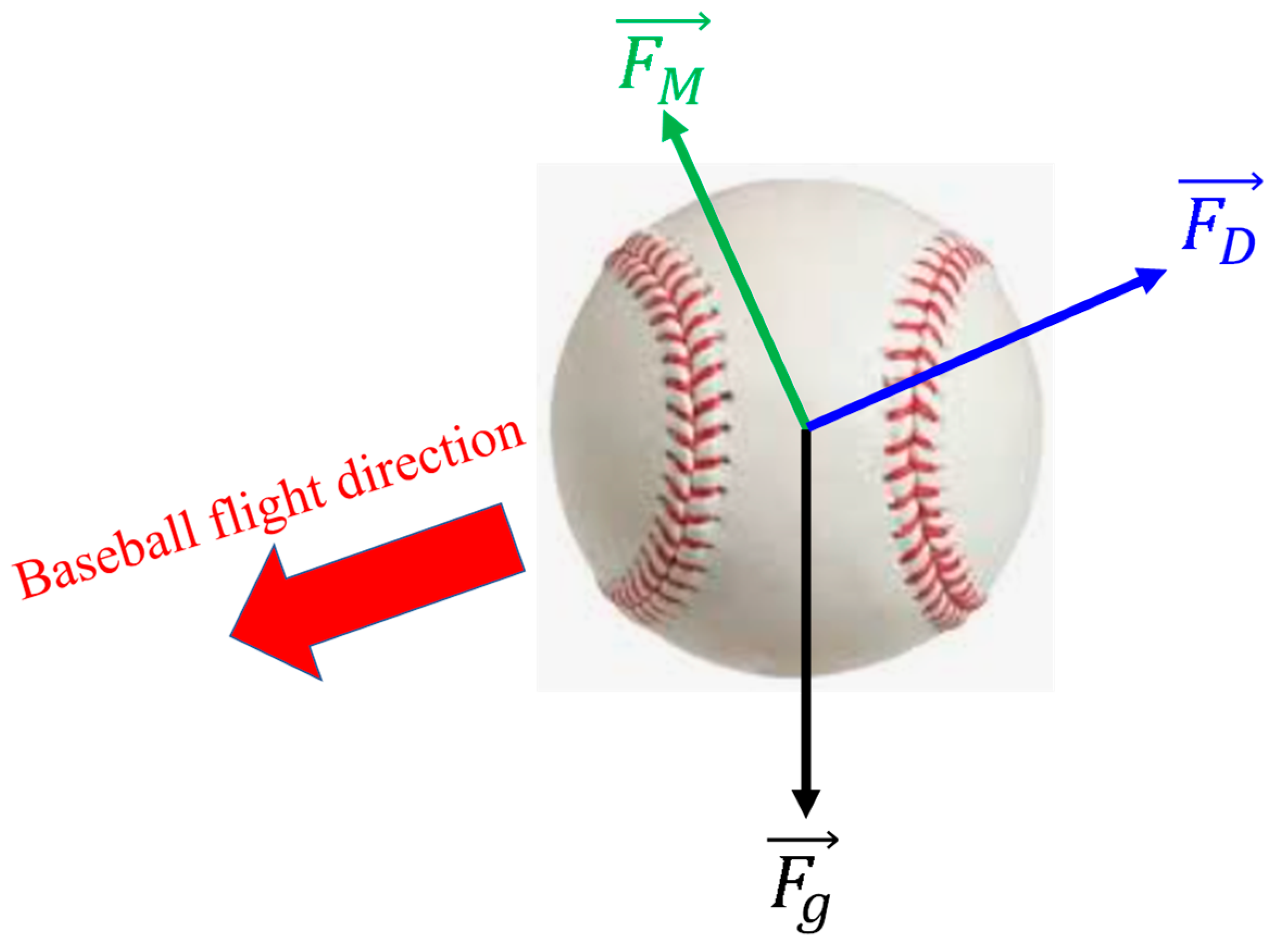
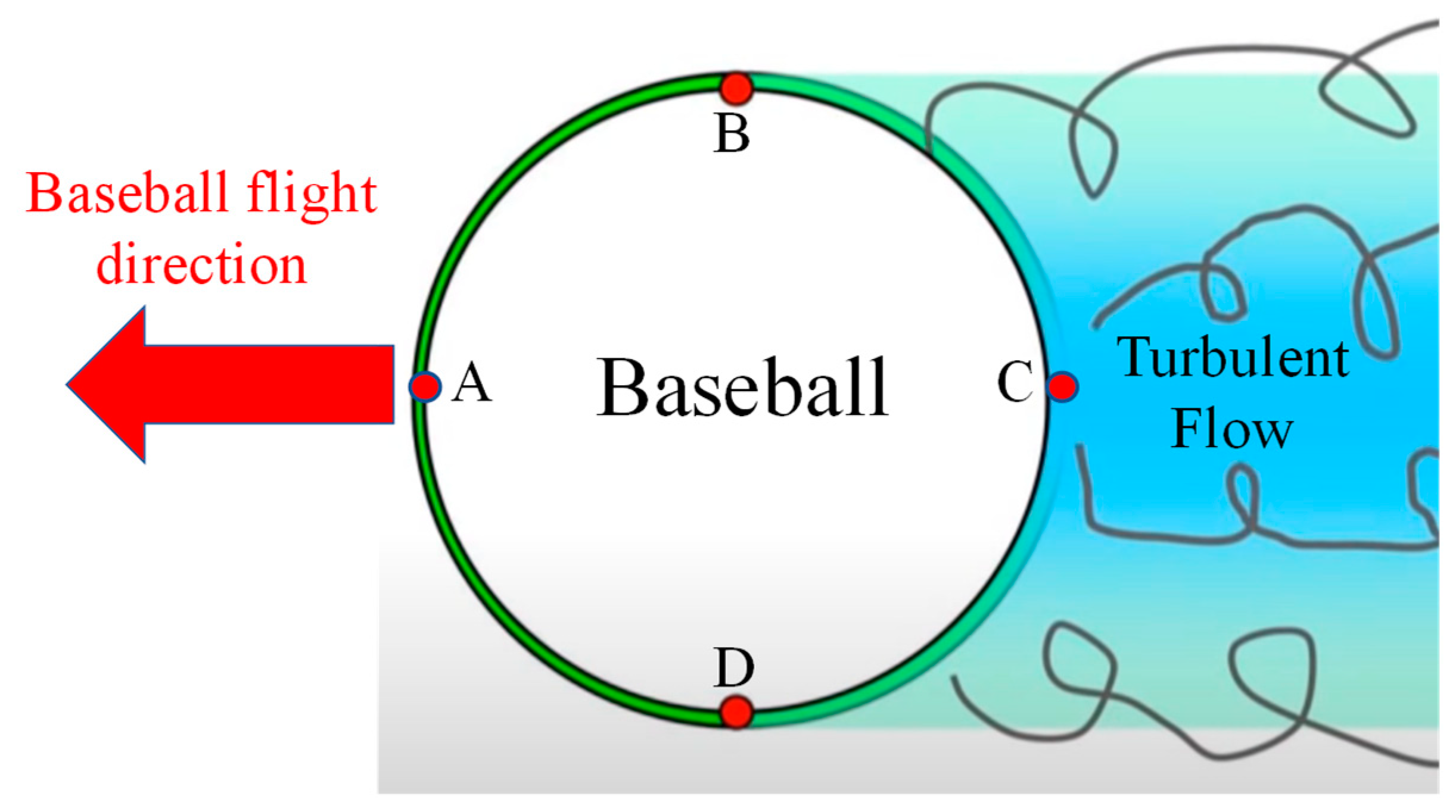
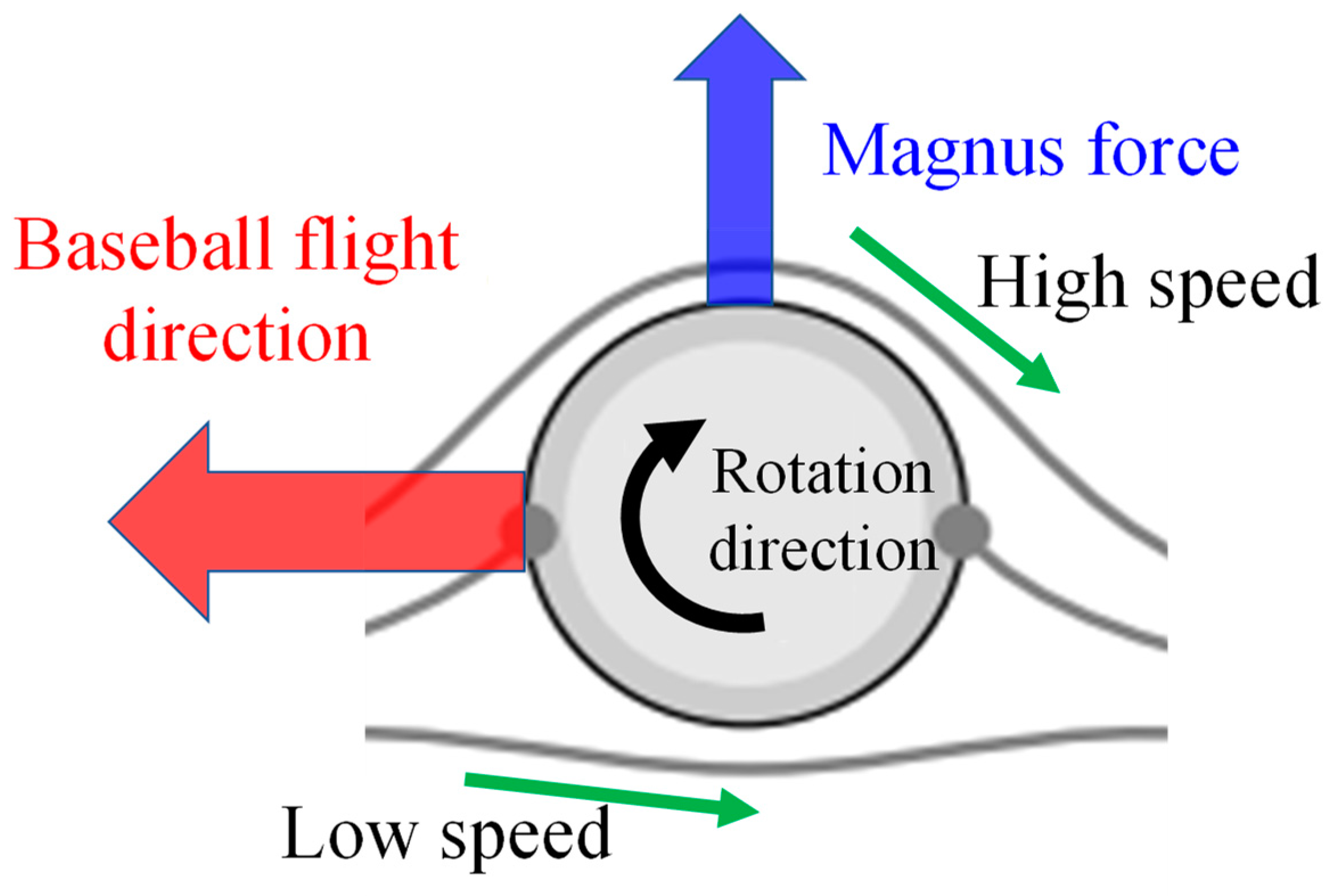
2.1. Dynamic Analysis of a Pitched-Baseball Trajectory Using Aerodynamic Theory

A baseball in flight is mainly affected by the gravitational force F g , force of air resistance F D , and Magnus force F M , as shown in Figure 1. To simplify the calculation, this study has ignored the influence of the wind direction on the baseball.
The boundary-layer theory proposed by Ludwig Prandtl describes the interaction between a flying baseball and air [6]. When air flows across the surface of the baseball, friction occurs. As air is a viscous fluid, the velocity gradually decreases to zero as it approaches the surface of the baseball, and the area in which this happens is called the boundary layer. Due to the viscous force within the boundary layer, Bernoulli’s principle is not applicable. The flow outside the boundary layer is closer to the inviscid flow and can be regarded as an ideal fluid to which the Bernoulli’s principle can be applied. As shown in Figure 2, the green area is the boundary layer, and the line segment is the fluid streamline. According to Bernoulli’s principle, the fluid velocity from A to B (or A to D) increases outside the boundary layer, and the fluid velocity from B to C (or D to C) decreases. It can be seen that points A and C are high-pressure points, and points B and D are low-pressure points. When the pressure difference is sufficiently large, the boundary layer flows back and creates a separation point, and boundary-layer separation occurs from B to C (or D to C). As shown in Figure 2, the fluid instability after the separation point (points B and D) is called turbulent flow. Compared to the entire flow field, the turbulent flow is a low-pressure area. The pressure difference between the turbulent flow area and the rest of the flow field is the main cause of the air resistance. The air resistance is in the opposite direction of the baseball flight, and through dimensional analysis [4] the baseball air resistance formula is obtained as
F D = 1 2 C D ρ A v 2 ( v v ) ,
where C D is the drag coefficient, ρ is the air density, A is the cross-sectional area of the baseball, and v is the ball speed. The value of the drag coefficient C D is 0.3 from a wind tunnel experiment [28].
According to fluid mechanics [4], it can be assumed that the flying baseball is a rotating cylinder placed in a fluid field. As the real fluid is viscous, the fluid in contact with the rotating cylinder exhibits the same rotational speed as that of the cylinder, as shown in Figure 3. In Figure 3, according to Bernoulli’s principle, the flow velocity increases, and the pressure decreases above the ball and vice versa below the ball, assuming that the baseball is rotating clockwise. This pressure difference causes the ball to shift upwards, and this phenomenon is the Magnus force effect. For a flying baseball, a Magnus force effect is generated when the sphere rotates. Although the complicated interaction between the seams of the baseball and the boundary layer causes the Magnus force to change over time, it can be averaged according to the Magnus force formula as follows [29]:
F M = 1 2 C M ρ A v 2 ( ω × v ω v ) ,
C M = { 1.5 S   , S 0.1 0.09 + 0.6 S   , S > 0.1 ,
where C M is the Magnus coefficient, ω is the angular velocity, S = R ω v is the spin parameter, and R is the radius of the baseball.
The pitching image angle provided by the broadcasting unit camera makes the analyses of the horizontal displacement of the baseball flight and the baseball rotation axis very different. Therefore, this study assumed that the rotation axis of the baseball is horizontal and has only analyzed the types of baseballs that have been subjected to vertical displacement, including four-seam fastballs, forkballs, and change-up balls, and then analyzed the flying force of the baseballs in a two-dimensional plane. The viewing angle and position of the pitching image based on the broadcast unit were fixed. This study assumed that the x-axis is in the rightmost connection direction, and the y-axis is in the vertical direction in the image of the pitcher board and the home plate (Figure 4). In addition, we defined the rightmost point of the pitcher board as the origin of the image coordinate system, as shown in Figure 4. Therefore, the baseball force is:
F x = F D x + F M x = ( 1 2 C D ρ A v x 2 ) + ( 1 2 C M ρ A v 2 s i n θ ) s i n θ ,
F y = F D y + F g + F M y = ( 1 2 C D ρ A v y 2 ) + ( m g ) + ( 1 2 C M ρ A v 2 s i n θ ) c o s θ ,
where m is the weight of the ball, g is the acceleration due to gravity, and θ = tan 1 y 2 y 1 x 2 x 1 is the pitch angle. The coordinates of the baseball at the throw point of the pitcher are ( x 1 , y 1 ).   x 1 , y 1 and x 2 , y 2 are the flight distances and heights of the ball at t 1 and t 2 , respectively.
As this study only considers the Magnus force effect in the y-direction, Equation (5) can be rewritten as
F y = F D y + F g + F M y = F D g + F M y ,
where F D g = F D y + F g . When the time is t , the average acceleration, velocity, and displacement in the y-direction caused by air resistance and gravity are as follows:
a D g = ( 1 2 C D ρ A v y 2 m g ) / m ,
v D g ( t ) = v D g ( t 1 ) + a D g t ,
y D g ( t ) = y D g ( t 1 ) + v D g ( t 1 ) Δ t + 1 2 a D g t 2 .
In addition, the average acceleration, velocity, and displacement in the y-direction caused by the Magnus force are as follows:
a M y = ( ( 1 2 C M ρ A v 2 s i n θ ) c o s θ ) / m ,
v M y ( t ) = v M y ( t 1 ) + a M y t ,
y M y ( t ) = y M y ( t 1 ) + v M y ( t 1 ) Δ t + 1 2 a D g t 2 .
Finally, this study used deep learning algorithms to recognize the baseball and calculated the y-axis displacement ∆y (late break) between the pitcher’s throw and the catcher’s catch from the broadcast unit image as follows:
Δ y = y D g + y M y .
As y D g can be obtained from Equation (9), y M y can be obtained using Equation (13). Finally, from Equations (2), (3), and (10) to (12), the angular velocity ω of the flying baseball can be obtained as follows:
ω = 1 R ( 4 m t 2 C M ρ A s i n θ c o s θ ( y D g + y M y ( t 1 ) + v M y ( t 1 ) Δ t Δ y ) ) 1 / 2 .
The average ball speed v A of the baseball flight between time t i (when thrown by the pitcher) and t e (when received by the catcher) can be obtained as follows:
v A = x e x i t e t i ,
where x i is the x-axis coordinate of the pitcher throw, x e is the x-axis coordinate of the catcher receive, and this study assumed that x e x i is the distance from the pitcher board to the home plate (18.44 m).

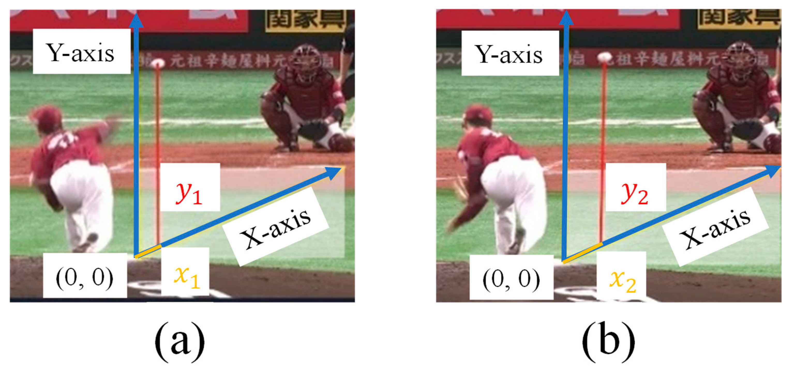
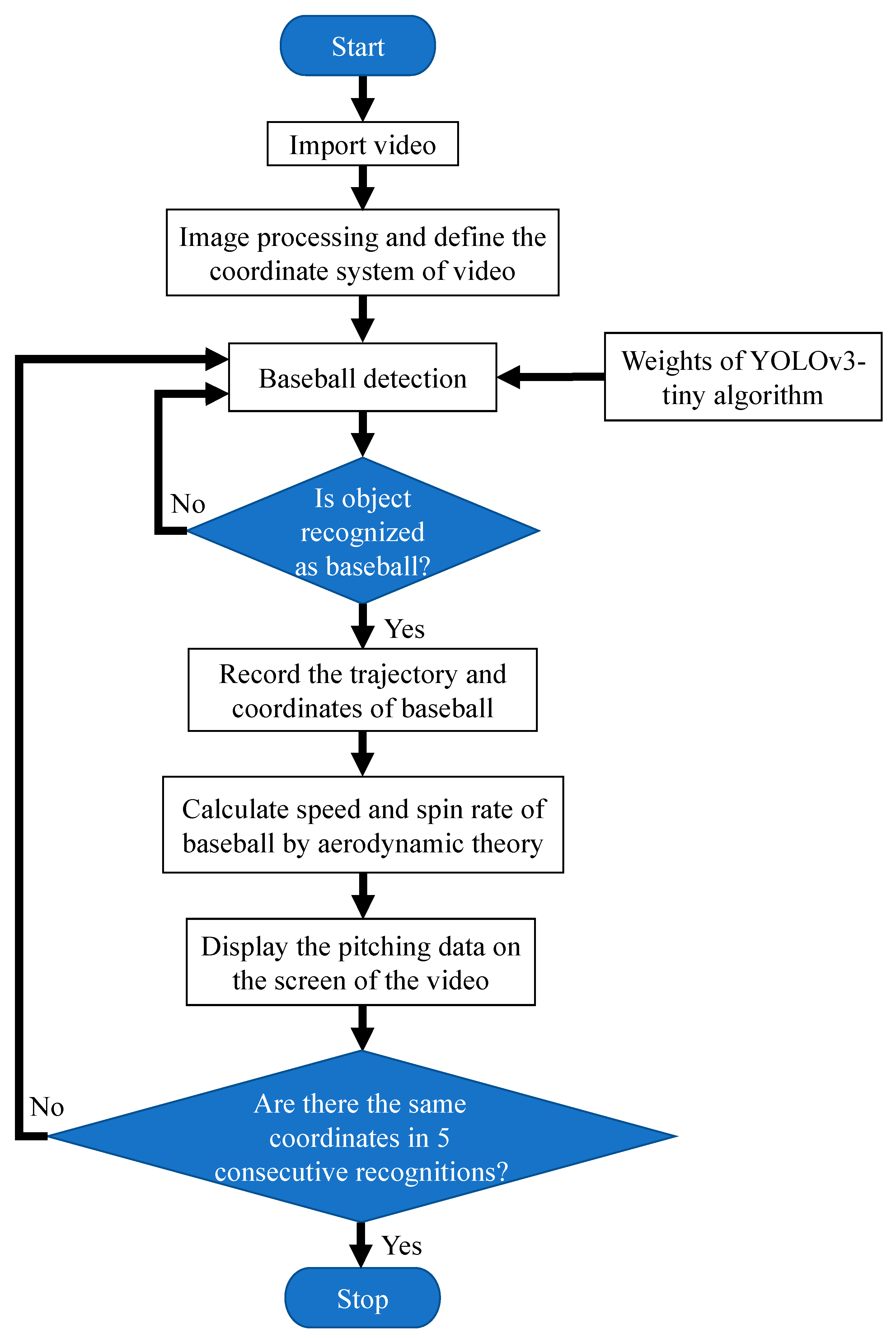
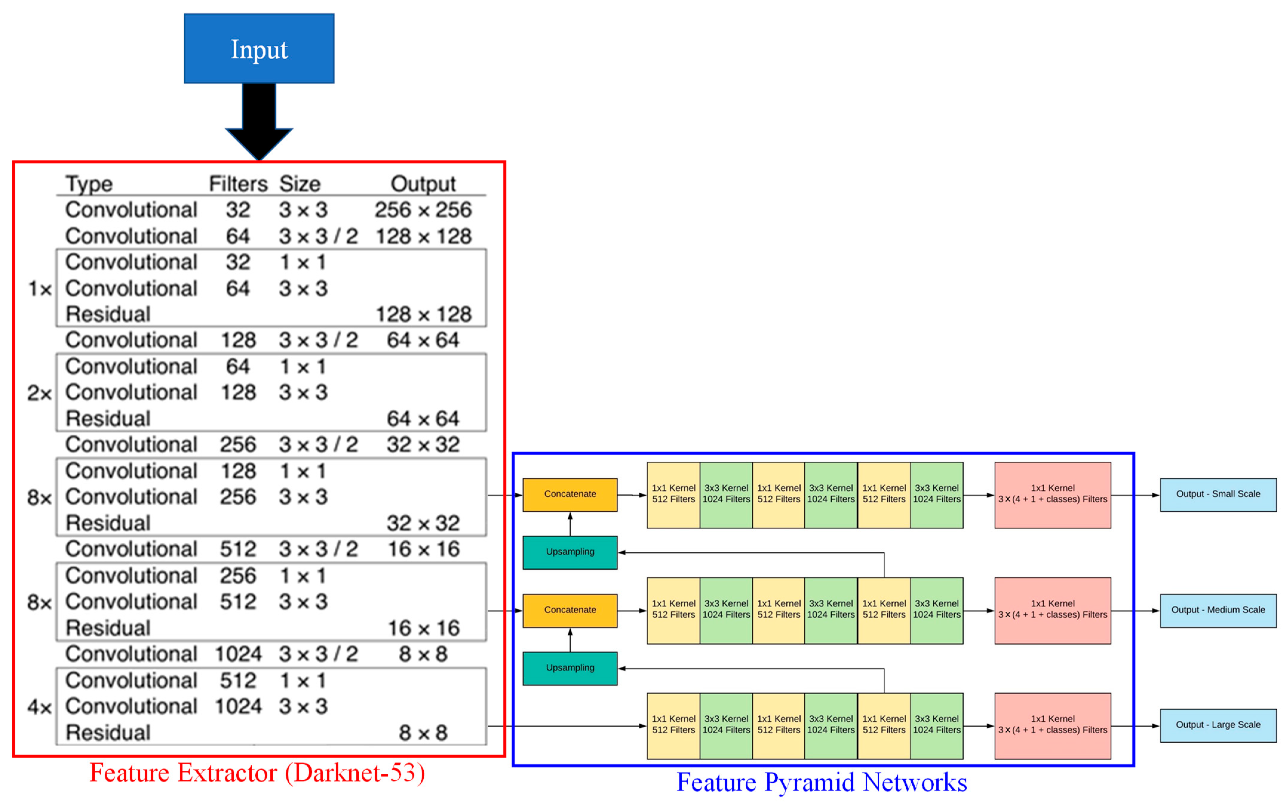
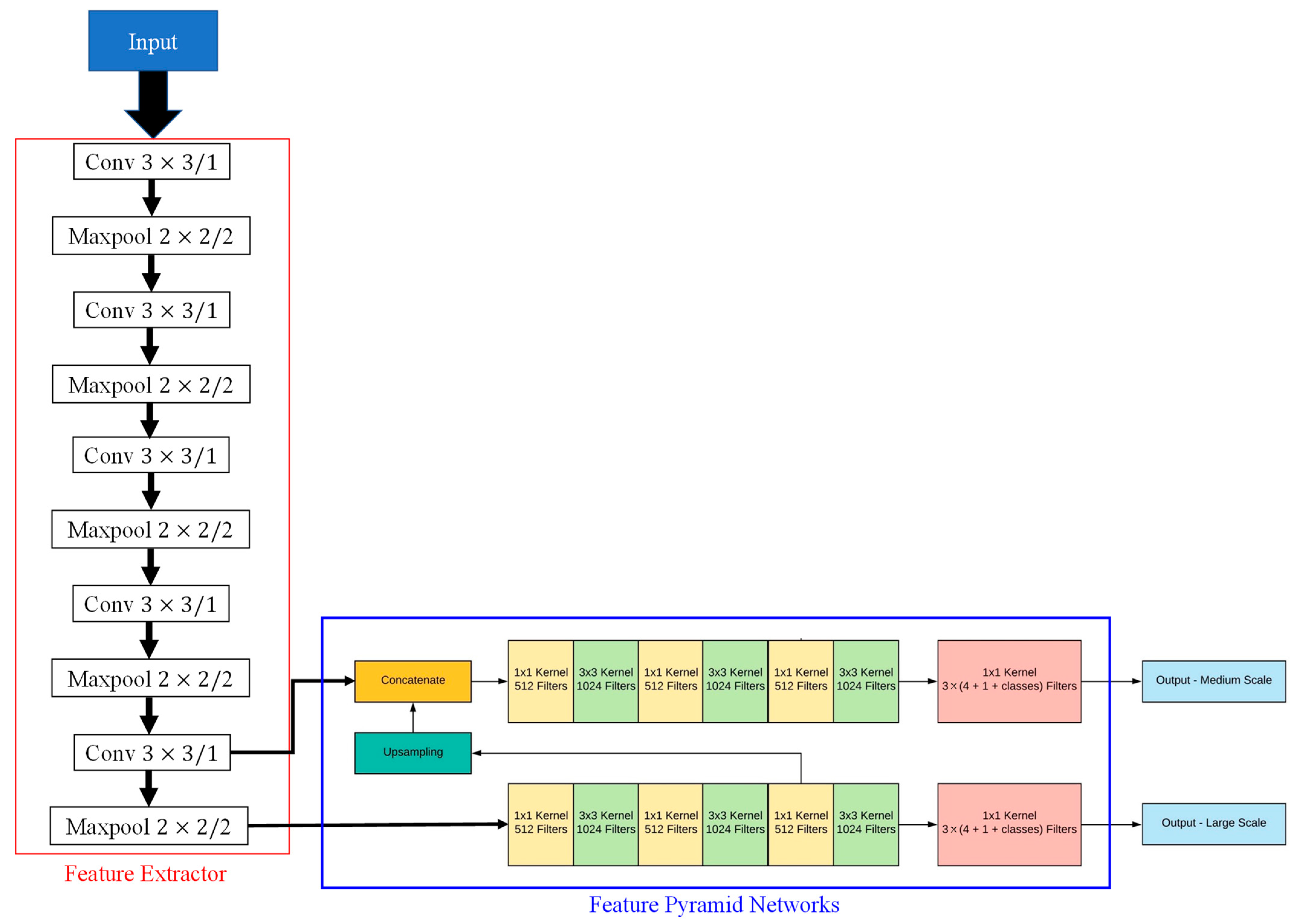
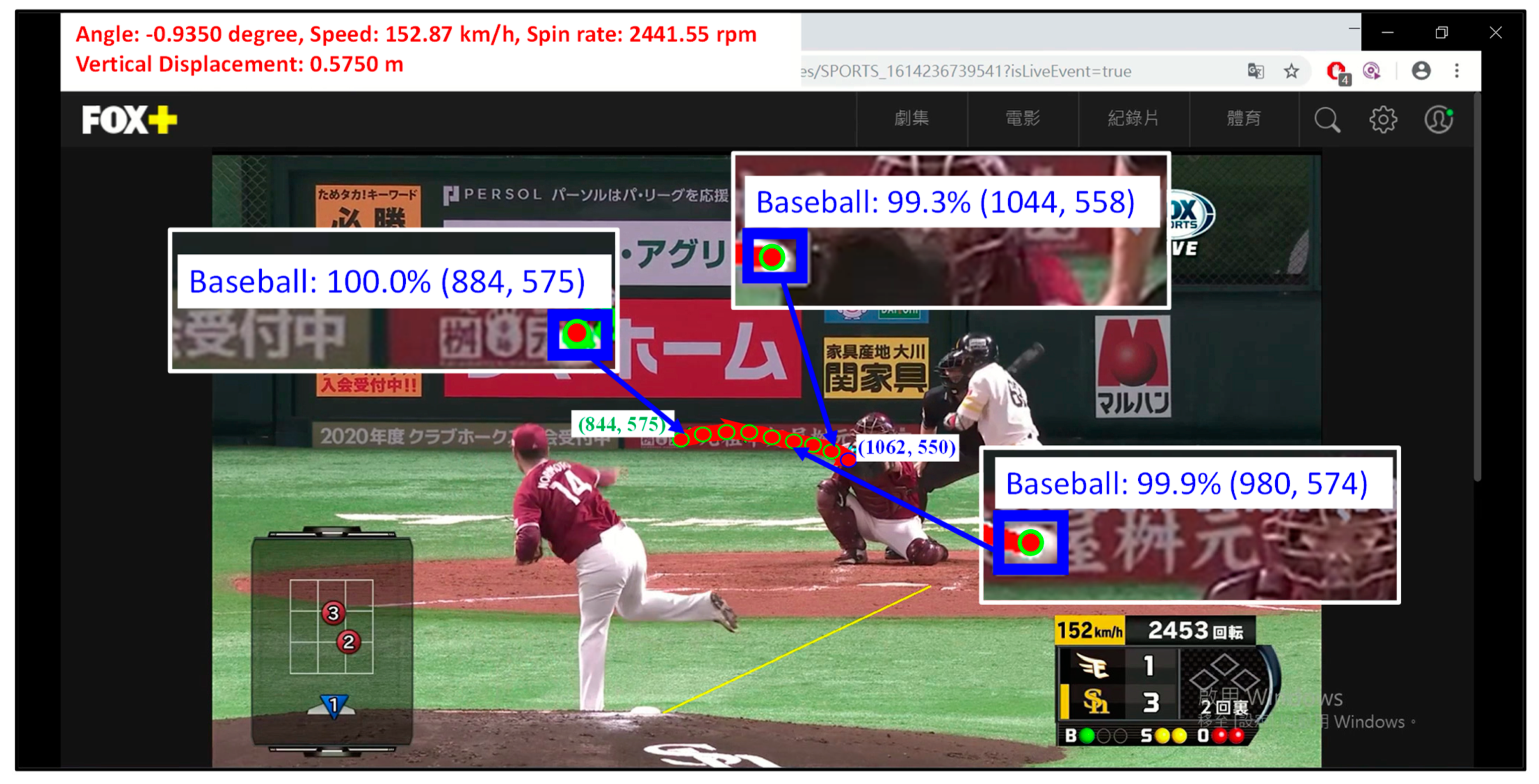
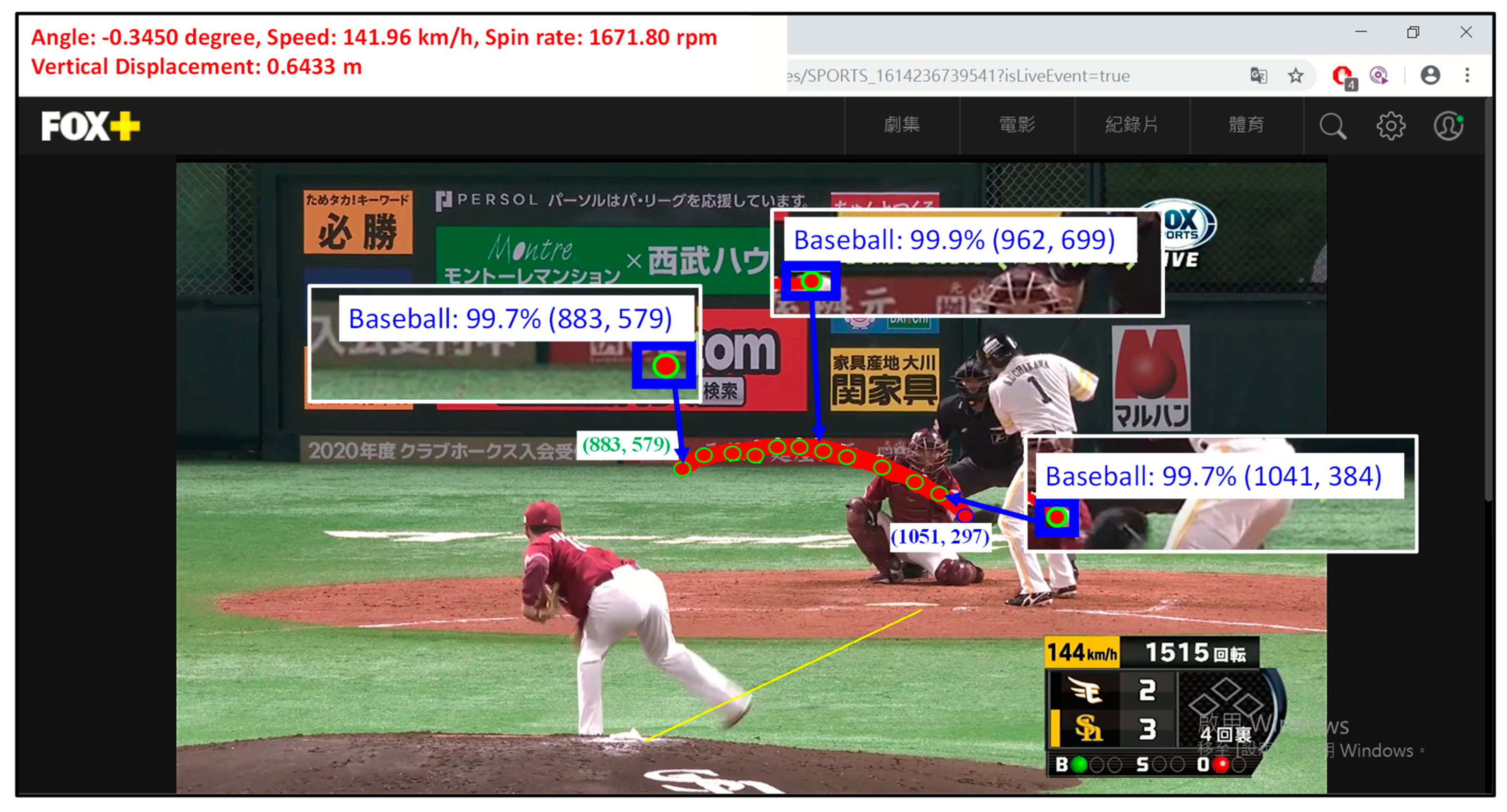
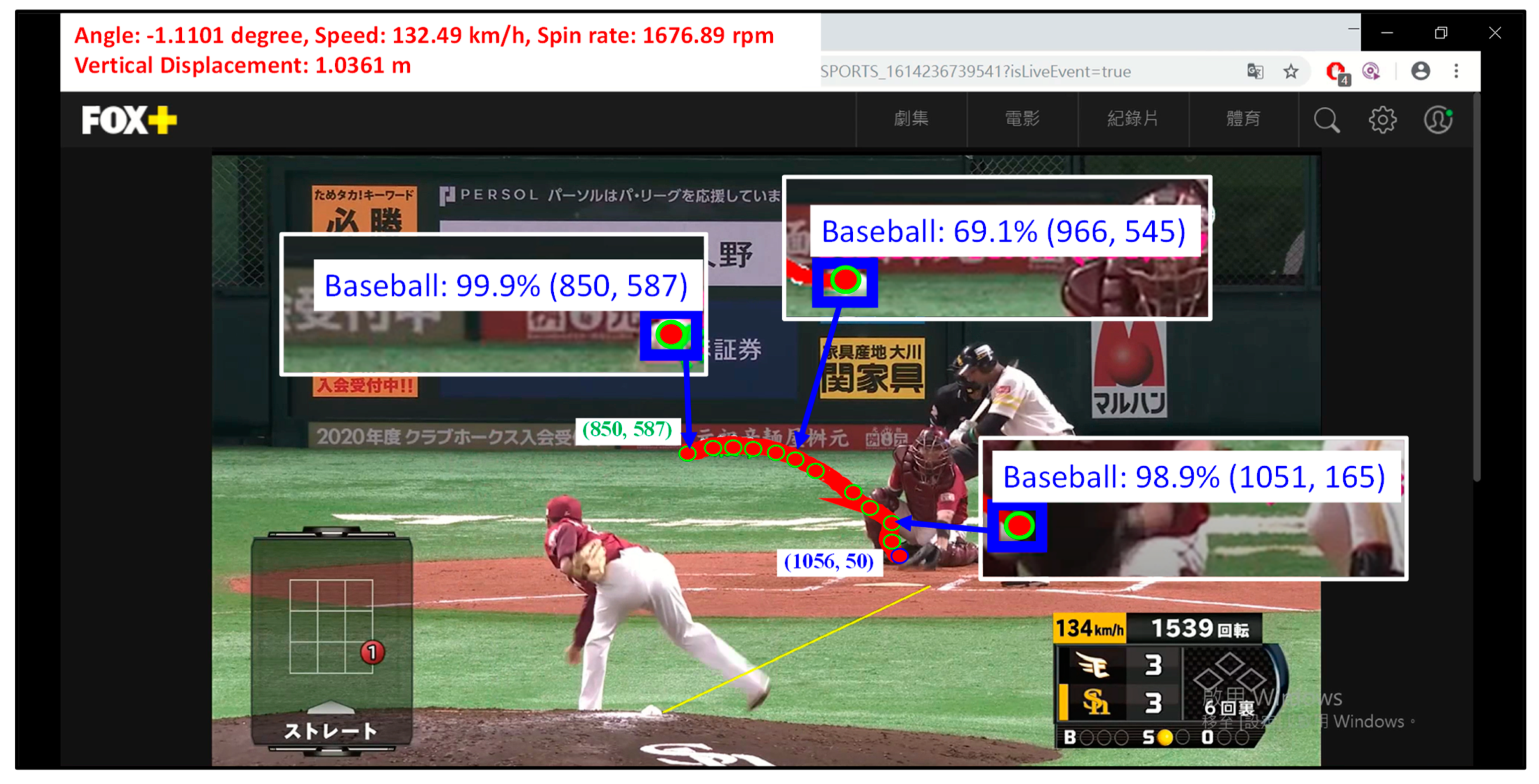
2.2. Recognition of a Pitched-Baseball Trajectory by Deep Learning Algorithm

To analyze the results of the ball speed and spin rate of the baseball through aerodynamic theory, this study used the YOLOv3 deep learning algorithm to recognize the baseball and its flight trajectory. YOLOv3, the third generation of YOLO, has the advantages of the previous generations’ algorithms and has an updated multi-scale detection function and a more powerful feature extraction network. Therefore, it can detect objects of different scales simultaneously, thereby improving the accuracy and performance. The YOLOv3 algorithm is divided into the following two major parts [17]: (1) feature extraction and (2) multi-scale detection. The architecture of YOLOv3 is illustrated in Figure 5. The feature extractor of YOLOv3 is Darknet-53, which was modified from Darknet-19 used by YOLOv2 [30]. Using the concepts of residual network, ResNet, and residual learning, it avoids the gradient diminishing problem by increasing the number of network layers for more complex feature extraction.
In the multi-scale detection portion, YOLOv3 uses feature pyramid networks (FPNs) upgraded from the original single-layer 13 × 13 feature prediction network to a three-layer 13 × 13, 26 × 26, and 52 × 52 feature prediction network. The single layer of five bounding boxes is changed to three layers of three bounding boxes each, which is equivalent to a total of nine bounding boxes. The FPN architecture merges the better target at the lower level with the better semantic features at the higher level and makes independent predictions at different feature levels, showing an obvious improvement in small object detection. YOLOv4 [24,25,26] utilizes a spatial pyramid pooling and path aggregation network to improve the performance of YOLOv3.
However, because the baseball thrown by the pitcher is fast and live-action TV videos like sports and concerts are typically at least 24 fps or more [27], this study used YOLOv3-tiny algorithm to speed up the calculation [18]. To speed up the calculation, this study further used YOLOv3-tiny to recognize the baseball and its flight trajectory. YOLOv3-tiny is a simplified version of YOLOv3, as shown in Figure 6. The backbone network of Darknet-53 is simplified to a network similar to that of Darknet-19, and the 52 × 52 small object prediction branch and its feature layer have been omitted, leaving only two independent prediction branches. Although the accuracy is not as high as that of YOLOv3 and YOLOv4, the calculation becomes extremely fast [19,23,26]. The efficiency and accuracy of the calculation were sufficient for the identification and tracking of the baseballs used in this study. In the next section, this study has compared the performance of models trained by YOLOv3 and YOLOv4 with that of a model trained by YOLOv3-tiny algorithm.

3. Experiments

To use the deep-learning algorithm to recognize the baseball and its flight trajectory, this study used 485 screenshots of the baseball TV broadcast. Among them, 80% of the screenshots (388 sheets) were randomly selected as training data sets, and the remaining 20% (97 sheets) were used for verification. In addition, this study sets the hyperparameters to a learning rate of 0.001, a mini-batch size of 64, a momentum of 0.9, and weight decay of 0.0005. First, the size of the input image was adjusted. As the resolution increases, the detection of small objects improves, but the computational load increases, and the computational speed decreases during training. Therefore, this study used a 416 × 416-pixel (referred to as the tiny-416 model) and a 608 × 608-pixel (referred to as the tiny-6081 model) resolution to analyze the baseball recognition capability by YOLOv3-tiny. Moreover, the intersection over union (IoU) and mean average precision (mAP) were used to compare and analyze the accuracy [20,24,25,31,32]. IoU is the intersection of the combined points of the predicted and actual frames. In this study, the object was considered to be successfully recognized when the IoU was greater than 0.5. Additionally, the calculations of mAP, Precision, Recall, and F1-score based on the IoU of 0.5 is as follows:
mAP = AP N C ,
where N C is the target type. AP is
AP = Precision N ,
where N is the number of pictures. Precision, recall, and F1-score are expressed as
Precision = TP TP + FP ,
Recall = TP TP + FN ,
F 1 = 2 × Precision × Recall Precision + Recall ,
where TP is a positive sample that is correctly classified, FP is a positive sample that is misclassified, and FN is a negative sample that is misclassified. Regarding the tiny-416 and tiny-6081 models, based on the results of 6000 epochs of training experiments, it is clear that the IoU, precision, recall, F1-score, and mAP of the tiny-6081 model are better than those of the tiny-416 model, as shown in Table 1. This verifies that the larger the resolution of the picture, the better the recognition of the small objects. In addition, the number of training epochs is positively correlated with accuracy, but numerous monotonic samples may lead to overfitting, making it difficult to identify images that are not in the training set. Therefore, this study adjusted the number of training epochs from 6000 (tiny-6081 model) to 12,000 (tiny-6082 model) in the initial training by YOLOv3-tiny. Table 1 shows that the IoU, precision, recall, F1-score, and mPA of the tiny-6082 model are better than those of the tiny-6081 model. In addition to using YOLOv3-tiny, this study trained a model using YOLOv3 as well for comparison purposes. In the comparative experiment, the input image was trained with 12,000 epochs at the 416 × 416 (v3-416 model) and 608 × 608 (v3-608 model) resolutions by YOLOv3, and the 608 × 608 (v4-608 model) resolution by YOLOv4. The training results in Table 1 show that the IoU, precision, recall, F1-score, and mPA of the v3-416, v3-608, and v4-608 models are better than those of the tiny-6082 model. Moreover, the performance of the v4-608 model by YOLOv4 is the best of all models in Table 1. However, the execution speed of the tiny-6082 model is approximately 2.5 times that of the v3-416, v3-608, and v4-608 models. Additionally, the execution speeds of the v3-416, v3-608, and v4-608 models perform below 20 fps. Live-action TV videos like sports and concerts are typically at least 24 fps or more [27]. Therefore, this study utilized the tiny-6082 model with an image resolution of 608×608 pixels and 12,000 epochs of training set to complete the recognition of the baseball and its flight trajectory. Python software was used to analyze 30 testing videos of a pitched baseball using the YOLOv3-tiny deep learning algorithm for flight trajectory, ball speed, and spin rate, as shown in Figure 7.
First, after importing the video, the program defined the coordinate system of the video. Second, baseballs were recognized using the YOLOv3-tiny algorithm. After the pitcher throws the ball, the coordinate of the first recognized baseball object was recorded and presented as a point on the video screen. Third, the baseball was recognized at subsequent points in its trajectory in sequence. The coordinate of each recognized baseball position was marked, and all the points were connected with a line to complete the presentation of the ball flight trajectory. Fourth, according to the coordinates of the baseball positions recorded in each frame, the program started to find the point where the baseball was captured (captured point) when the number of recorded points was greater than five. When the coordinates of the baseball were observed to be the same for five consecutive frames, the program determined it as the captured point. Finally, the ball speed and spin rate were calculated using the aerodynamic theory and physical parameters (Table 2) of the pitched baseball, and they were presented on the screen to complete the calculation and recording of the pitched-baseball flight trajectory, vertical displacement, ball speed, and spin rate.

4. Results and Discussion

To obtain a comparative standard value for the measurement data of the pitcher’s ball speed and spin rate, this study used 30 home-game videos of the Fukuoka Softbank HAWKS baseball team, including real-time displays of the ball speed and spin rate by the Fox Networks Group. The testing videos of the pitched baseballs included four-seam fastballs, forkballs, and change-up balls. This automatic measurement and analysis system of pitched-baseball trajectories showed the pitch angle, speed, spin rate, vertical movement, and other information of the flying baseball in real time. Moreover, this study made a numerical comparison of the measurement results with the ball speed and spin rate provided by the broadcasting unit, and the related automatic measurement results are shown in Figure 8, Figure 9 and Figure 10 and Table 3. In Figure 8, Figure 9 and Figure 10, the measurement results of this study are shown in the upper left corner, and the measurement results of the broadcast unit are shown in the lower right corner. The trajectories and the coordinates of the throw point and catch point of the pitched baseball are represented for four-seam fastball, forkball, and change-up ball in Figure 8, Figure 9 and Figure 10, respectively. The three bounding boxes with classification confidences and coordinates of the ball by YOLOv3-tiny in the trajectory of pitched baseball are depicted in Figure 8, Figure 9 and Figure 10, respectively. Most values of classification confidence in this study are close to 100%. However, the worst classification confidence of 69.1% is presented in Figure 10, because the ball was flying between a red billboard and green grass when the ball in the video was recognized. According to the measurement results in Table 3, this algorithm accurately recorded the trajectory of the ball. The average error of the measured ball speed was 1.88% with a standard deviation of 1.16, and the average error of the measured spin rate was 7.51% with a standard deviation of 4.33.
According to Equation (15), the ball speed estimation method in this study is related to the number of frames per second (fps) of the video. The test video in this study was at 30 fps, and the single-frame interval was 0.0334 s. Errors between the measured ball speed and the actual ball speed are due to the minimum measurement resolution of the time parameter in the denominator of Equation (15). In addition, the spin rate estimation using Equation (14) and the pitch angle have a significant correlation. The detection of the ball at the moment of the pitcher’s throw can easily cause a sensing error, which causes an error in the calculation of the pitch angle, ultimately leading to an error between the measured spin rate and the actual spin rate. In addition, as seen from the measured results in Table 3, the ball speeds of the four-seam fastballs are in the range of 145–154 km/h, and the spin rates are the highest among the three pitch types, ranging from 2082 to 2477 rpm. Moreover, the Magnus displacements are between 0.64 and 0.72 m in the upward direction. The ball speeds of the forkballs are between 134 and 144 km/h, the spin rates are between 976 and 1515 rpm, and the Magnus displacements are between 0.45 and 0.58 m in the upward direction, which were the smallest among the three pitch types. Due to the downward displacement caused by air resistance and gravity, a small Magnus displacement results in a large downward displacement of the forkball. Finally, for the change-up ball, the ball speeds are between 133 and 138 km/h (slowest among the three pitch types), the spin rates are between 1539 and 2009 rpm, and the Magnus displacements are between 0.59 and 0.69 m in the upward direction. From Table 3 and Equation (13) it is clear that the smaller the Magnus displacement of the ball, the larger the longitudinal displacement when the ball reaches home base. This also means that there is a larger late break. According to Equations (10)–(12), the Magnus displacement is related not only to the physical parameters of the baseball, but also, more importantly, to the pitch angle, ball speed, and spin rate. Therefore, according to the Magnus displacements, ball speeds, spin rates listed in Table 3, and a least-square fitting algorithm from IEEE Standards [33], the curve-fitting equation between the Magnus displacement and ball speed was obtained with a coefficient of determination (R2) of 0.30. Furthermore, the curve-fitting equation between the Magnus displacement and spin rate was also obtained with an R2 of 0.71, showing a positive correlation between the Magnus displacement and spin rate. As the pitching skill of every pitcher is different, the spin rate of the ball may be different for different pitchers even for the same pitch types and ball speed. Therefore, in this study, the spin rate was divided by the ball speed, and the curve fitting of this ratio was done with the Magnus displacement. The curve-fitting equation [33] between the Magnus displacement and the ratio of the spin rate to the ball speed was obtained with an R2 of 0.78. Compared to the spin rate alone, the ratio of the spin rate to the ball speed was found to be more positively correlated with the Magnus displacement. For this reason, this ratio was a more effective parameter for analyzing the late break of the pitcher. This study analyzed the Nippon Professional Baseball (NPB) match between the Tohoku Rakuten Golden Eagles and the Fukuoka Softbank HAWKS baseball team on 6 October 2019. Furthermore, this technology was used to analyze the pitching state of the four-seam fastball of the starting pitcher (Manabu Mima), as shown in Table 4. Manabu Mima pitched a total of four innings in this game using 62 balls. The speeds of his four-seam fastballs were between 137 and 147 km/h, and the spin rates were between 2219 and 2495 rpm. The parameter of the spin rate to ball speed ratio was between 15.10 and 18.21. According to the results of the previous discussion, the smaller this parameter, the larger the late break phenomenon. Therefore, according to the results in Table 4, this parameter for Manabu Mima increases in the four-seam fastballs from the 27th to 48th ball, which also means that the late break of this pitcher decreases. According to the actual game situation of the 27th to 48th ball (in the third inning), Manabu Mima lost three points in this inning. Additionally, this study analyzed the MLB matches on 14 and 18 April 2022, respectively, as shown in Table 5 and Table 6. Shohei Ohtani (the starting pitcher of the Los Angeles Angels baseball team) pitched a total of 3.2 innings in this game using 70 balls in the match on 14 April 2022. The speeds of his four-seam fastballs were between 154 and 158 km/h, and the spin rates were between 2157 and 2395 rpm. The parameter of the spin rate to ball speed ratio was between 13.93 and 15.59. According to the results in Table 5, this parameter for Shohei Ohtani increases in the four-seam fastballs from the 10th to the 36th ball and after the 62nd ball, which also means that the late break of this pitcher decreases. According to the actual game situations of the 10th to 36th ball (in the second inning) and the 62th to 70th ball (in the fourth inning), Shohei Ohtani lost four and two points in the second and fourth innings, respectively. In the match on 18 April 2022, Clayton Kershaw (the starting pitcher of the Los Angeles Dodgers baseball team) pitched a total of 5 innings in this game using 87 balls. The speeds of his four-seam fastballs were between 143 and 146 km/h, and the spin rates were between 2310 and 2467 rpm. The parameter of the spin rate to ball speed ratio was between 16.01 and 17.23. According to the results in Table 6, this parameter for Clayton Kershaw increases in the four-seam fastballs from the 59th to 81se ball, which also means that the late break of this pitcher decreases. According to the actual game situation of the 59th to 81st ball (from the fifth to sixth innings), Clayton Kershaw lost one and three points in the fifth and sixth innings, respectively. Therefore, it was verified through the parameter of the spin rate to ball speed ratio that the late break of the pitcher became smaller, thereby reducing the power of pitching.

5. Conclusions

In this study, pitched-baseball characteristics were analyzed to observe the effects of Magnus force on a pitched-baseball trajectory from TV broadcast videos using the aerodynamic theory. Moreover, an automatic measurement and analysis system was established by YOLOv3-tiny for the pitched-baseball trajectories, speeds, and spin rates. Finally, a system was used to automatically present pitching data, such as the throw point, catch point, pitch angle, ball speed, spin rate, vertical displacement, and ball trajectory on the screen. According to the results of 30 testing videos of pitched baseballs, this system fully grasped the baseball trajectories, throw points, catch points, and vertical displacements. The average errors of the measured ball speeds and spin rates were 1.88% and 7.51%, respectively, compared to the values of the ball speeds and spin rates provided by the TV broadcast. In addition, this study used the ratio of the spin rate to the ball speed as a parameter to analyze the pitching state of the pitcher’s four-seam fastballs. It can be seen from the results of the NPB and MLB matches that when this parameter increased, the Magnus displacement of the ball also increased, thereby decreasing its late break. As a result, the spin rate to ball speed ratio verified that the late break of the pitcher became smaller, and thus the power of pitching reduced. Using this system, pitching information in the baseball game was easily obtained and recorded for further discussion. The system developed in this study provides scientific pitching data to improve the performance of baseball pitchers.

Author Contributions

Conceptualization, B.-J.W.; methodology, B.-J.W., C.-R.C., C.-W.L. and Y.-C.Z.; software, B.-J.W., C.-R.C., C.-W.L. and Y.-C.Z.; validation, B.-J.W., C.-R.C., C.-W.L. and Y.-C.Z.; formal analysis, B.-J.W.; investigation, B.-J.W.; resources, B.-J.W.; data curation, B.-J.W., C.-R.C., C.-W.L. and Y.-C.Z.; writing—original draft preparation, B.-J.W.; writing—review and editing, B.-J.W.; visualization, B.-J.W.; supervision, B.-J.W.; project administration, B.-J.W.; funding acquisition, B.-J.W. All authors have read and agreed to the published version of the manuscript.

Funding

The authors wish to thank the National Science Council of Taiwan for financial supports (grant numbers: 110-2221-E-019 -058 -MY2).

Conflicts of Interest

The authors declare no conflict of interest.

References

  1. Lage, M.; Ono, J.P.; Cervone, D.; Chiang, J.; Dietrich, C.; Silva, C.T. Statcast dashboard: Exploration of spatiotemporal baseball data. IEEE Comput. Graph. Appl. 2016, 36, 28–37. [Google Scholar] [CrossRef] [PubMed]
  2. Kagan, D.; Nathan, A.M. Statcast and the baseball trajectory calculator. Phys. Teach. 2017, 55, 134–136. [Google Scholar] [CrossRef]
  3. Bailey, S.R.; Loeppky, J.; Swartz, T.B. The prediction of batting averages in major league baseball. Stats 2020, 3, 8. [Google Scholar] [CrossRef] [Green Version]
  4. Gerhart, P.M.; Gerhart, A.L.; Hochstein, J.I. Munson’s Fluid Mechanics, Global Edition; John Wiley & Sons, Inc.: Hoboken, NJ, USA, 2017. [Google Scholar]
  5. Higuchi, T.; Morohoshi, J.; Nagami, T.; Nakata, H.; Kanosue, K. The effect of fastball backspin rate on baseball hitting accuracy. J. Appl. Biomech. 2013, 29, 279–284. [Google Scholar] [CrossRef] [PubMed] [Green Version]
  6. BP Unfiltered: Is “Late Break” Real? Available online: https://www.baseballprospectus.com/news/article/19994/bp-unfiltered-is-late-break-real/ (accessed on 4 May 2022).
  7. Anderson, J.D. Ludwig Prandtl’s boundary layer. Phys. Today 2005, 58, 42–48. [Google Scholar] [CrossRef]
  8. Guéziec, A. Tracking pitches for broadcast television. Computer 2002, 35, 38–43. [Google Scholar] [CrossRef]
  9. Chen, H.T.; Chen, H.S.; Hsiao, M.H.; Tsai, W.J.; Lee, S.Y. A trajectory-based ball tracking framework with visual enrichment for broadcast baseball videos. J. Inf. Sci. Eng. 2008, 24, 143–157. [Google Scholar]
  10. Ijiri, T.; Nakamura, A.; Hirabayashi, A.; Sakai, W.; Miyazaki, T.; Himeno, R. Automatic spin measurements for pitched Baseballs via consumer-grade high-speed cameras. Signal Image Video Process. 2017, 11, 1197–1204. [Google Scholar] [CrossRef]
  11. López, A.; Cuevas, F.J. Automatic multi-circle detection on images using the teaching learning based optimisation algorithm. IET Comput. Vis. 2018, 12, 1188–1199. [Google Scholar] [CrossRef]
  12. Islam, S.S.; Dey, E.K.; Tawhid, M.N.A.; Hossain, B.M.A. CNN Based Approach for Garments Texture Design Classification. Adv. Technol. Innov. 2017, 2, 119. [Google Scholar]
  13. Gan, W.; Wang, S.; Lei, X.; Lee, M.S.; Kuo, C.C.J. Online CNN-based multiple object tracking with enhanced model updates and identity association. Signal Process. Image Commun. 2018, 66, 95–102. [Google Scholar] [CrossRef]
  14. Babaee, M.; Li, Z.; Rigoll, G.A. Dual cnn–rnn for multiple people tracking. Neurocomputing 2019, 368, 69–83. [Google Scholar] [CrossRef]
  15. Bai, Y.; Xu, T.; Huang, B.; Yang, R. Deep deblurring correlation filter for object tracking. IEEE Access 2020, 8, 68623–68637. [Google Scholar] [CrossRef]
  16. Jain, M.; Subramanyam, A.V.; Denman, S.; Sridharan, S.; Fookes, C. LSTM guided ensemble correlation filter tracking with appearance model pool. Comput. Vis. Image Underst. 2020, 195, 102935. [Google Scholar] [CrossRef]
  17. Zhao, L.; Li, S. Object detection algorithm based on improved YOLOv3. Electronics 2020, 9, 537. [Google Scholar] [CrossRef] [Green Version]
  18. Wang, Y.; Jia, K.; Liu, P. Impolite pedestrian detection by using enhanced yolov3-tiny. J. Artif. Intell. 2020, 2, 113. [Google Scholar] [CrossRef]
  19. Golcarenarenji, G.; Martinez-Alpiste, I.; Wang, Q.; Alcaraz-Calero, J.M. Efficient real-time human detection using unmanned aerial vehicles optical imagery. Int. J. Remote Sens. 2021, 42, 2440–2462. [Google Scholar] [CrossRef]
  20. Lawal, M.O. Tomato detection based on modified YOLOv3 framework. Sci. Rep. 2021, 11, 1447. [Google Scholar] [CrossRef]
  21. Wen, B.J.; Lin, Y.S.; Tu, H.M.; Hsieh, C.C. Health-diagnosis of electromechanical system with a principal-component bayesian neural network algorithm. J. Intell. Fuzzy Syst. 2021, 40, 7671–7680. [Google Scholar] [CrossRef]
  22. Wen, B.J.; Kao, C.H.; Yeh, C.C. Intelligent wearable device of auxiliary force using fuzzy-Bayesian backpropagation control. J. Intell. Fuzzy Syst. 2021, 40, 7981–7991. [Google Scholar] [CrossRef]
  23. Chang, L.; Chen, Y.T.; Wang, J.H.; Chang, Y.L. Modified Yolov3 for Ship Detection with Visible and Infrared Images. Electronics 2022, 11, 739. [Google Scholar] [CrossRef]
  24. Roy, A.M.; Bhaduri, J. Real-time growth stage detection model for high degree of occultation using DenseNet-fused YOLOv4. Comput. Electron. Agric. 2022, 193, 106694. [Google Scholar] [CrossRef]
  25. Roy, A.M.; Bose, R.; Bhaduri, J. A fast accurate fine-grain object detection model based on YOLOv4 deep neural network. Neural Comput. Appl. 2022, 34, 3895–3921. [Google Scholar] [CrossRef]
  26. Sozzi, M.; Cantalamessa, S.; Cogato, A.; Kayad, A.; Marinello, F. Automatic Bunch Detection in White Grape Varieties Using YOLOv3, YOLOv4, and YOLOv5 Deep Learning Algorithms. Agronomy 2022, 12, 319. [Google Scholar] [CrossRef]
  27. Herr, L. Television Goes Digital; Springer: New York, NY, USA, 2009. [Google Scholar]
  28. Briggs, L.J. Effect of spin and speed on the lateral deflection (curve) of a baseball; and the Magnus effect for smooth spheres. Am. J. Phys. 1959, 27, 589–596. [Google Scholar] [CrossRef]
  29. Sawicki, G.S.; Hubbard, M.; Stronge, W.J. How to hit home runs: Optimum baseball bat swing parameters for maximum range trajectories. Am. J. Phys. 2003, 71, 1152–1162. [Google Scholar] [CrossRef]
  30. Sharif, M.; Amin, J.; Siddiqa, A.; Khan, H.U.; Malik, M.S.A.; Anjum, M.A.; Kadry, S. Recognition of different types of leukocytes using YOLOv2 and optimized bag-of-features. IEEE Access 2020, 8, 167448–167459. [Google Scholar] [CrossRef]
  31. Xu, J.; Ma, Y.; He, S.; Zhu, J. 3D-GIoU: 3D generalized intersection over union for object detection in point cloud. Sensors 2019, 19, 4093. [Google Scholar] [CrossRef] [PubMed] [Green Version]
  32. Xu, Q.; Lin, R.; Yue, H.; Huang, H.; Yang, Y.; Yao, Z. Research on small target detection in driving scenarios based on improved yolo network. IEEE Access 2020, 8, 27574–27583. [Google Scholar] [CrossRef]
  33. IEEE Standard 1241-2000; IEEE Standard for Terminology and Test Methods for Analog-to-Digital Converters. IEEE: Piscataway, NJ, USA, 2000; pp. 25–29.
Figure 1. Force analysis during baseball flight.
Applsci 12 05540 g001
Figure 2. Analysis of Ludwig Prandtl’s boundary-layer theory during baseball flight.
Applsci 12 05540 g002
Figure 3. Magnus force effect during baseball flight.
Applsci 12 05540 g003
Figure 4. Schematic of the baseball flight at (a) t 1 and (b) t 2 .
Applsci 12 05540 g004
Figure 5. Architecture of YOLOv3.
Applsci 12 05540 g005
Figure 6. Architecture of YOLOv3-tiny.
Applsci 12 05540 g006
Figure 7. Flowchart of pitched-baseball analysis by YOLOv3-tiny algorithm.
Applsci 12 05540 g007
Figure 8. Automatic measurement result for a four-seam fastball.
Applsci 12 05540 g008
Figure 9. Automatic measurement result for a forkball.
Applsci 12 05540 g009
Figure 10. Automatic measurement result for a change-up ball.
Applsci 12 05540 g010
Table 1. Results of the network test comparison.
ModelYOLOv3-Tiny-416YOLOv3-Tiny-6081YOLOv3-Tiny-6082YOLOv3-416YOLOv3-608YOLOv4-608
IoU (%)53.764.568.773.473.978.2
Precision (%)61.986.589.197.697.299.8
Recall (%)53.885.189.295.497.899.1
F1 (%)57.685.889.196.597.599.5
mAP (%)62.787.190.498.997.899.1
Frame rate based on GPU (FPS)48.547.147.019.018.917.1
Table 2. Physical parameters of a pitched baseball.
Weight   of   Baseball   ( m ) Air   Density   ( ρ ) Radius   of   Baseball   ( R ) Acceleration   due   to   Gravity   ( g ) Drag   Coefficient   ( C D )
0.145 kg 1.2   kg / m 3 0.037 m 9.81   kg / m 2 0.3
Table 3. Measurement results of the pitched-baseball trajectories.
Pitch TypeSpeed (km/h)Spin Rate (rpm)Pitch Angle θ (deg) Δ y   ( m ) y D g   ( m ) y M y   ( m ) Measured Speed (km/h)Measurement Error of Speed (%)Measured Spin Rate (rpm)Measurement Error of Spin Rate (%)Spin Rate/Speed
Four-seam fastball1522453−0.940.581.25−0.671530.5724420.4515.97
1492319−0.440.471.13−0.651532.6020949.7013.70
14923200.210.260.95−0.691532.6025238.7516.50
1542314−2.030.951.62−0.681530.7322672.0314.83
1452418−2.381.141.82−0.681422.1023871.2816.81
1452386−2.141.071.74−0.681422.1021539.7715.17
1482329−1.360.781.44−0.661533.2923420.5615.32
1502306−1.710.881.53−0.651531.9124325.4615.91
1482323−1.370.791.45−0.661533.29204212.1013.36
1462272−0.610.571.23−0.661422.7723352.7716.45
1522282−1.570.821.49−0.671530.57272619.4617.83
1542306−1.910.911.55−0.641530.7322761.3014.89
1542311−2.251.021.67−0.651530.73205111.2513.42
1502082−2.391.141.79−0.651531.91235813.2615.42
1502261−2.511.151.83−0.671531.9124327.5615.91
1522131−2.531.161.81−0.641530.5723218.9215.18
1532180−2.171.021.67−0.651530.0823286.7915.23
1512418−0.910.591.29−0.701531.2425957.3216.98
1492416−1.310.741.45−0.701532.6025897.1616.94
1502477−1.040.631.35−0.721531.9125924.6416.96
Forkball1381498−0.310.721.29−0.571323.9916429.6112.39
1441515−0.350.641.22−0.581421.42167210.3611.78
1341380−0.600.901.46−0.561321.13151910.0711.47
1371193−1.931.321.83−0.501323.2911216.048.46
140976−1.501.191.65−0.451381.6010295.437.47
Change-up ball1341539−1.111.041.70−0.661321.1316778.9712.66
1381930−1.200.931.58−0.651323.99172610.5713.03
1332009−2.491.422.10−0.691320.38175112.8413.22
1341552−0.900.971.55−0.591321.1316596.8912.52
1381800−1.951.201.83−0.631323.9917293.9413.05
Average error1.88Average error7.51
Standard deviation of error1.16Standard deviation of error4.33
Table 4. Pitching state analysis of four-seam fastballs by Manabu Mima.
Number of Pitches4792731323536484958
Speed (km/h)144147146147145146143143137147143
Spin rate (rpm)23982241235722192313238624152486249524412284
Spin/speed16.6515.2416.1415.1015.9516.3416.8917.3818.2116.6115.97
Table 5. Pitching state analysis of four-seam fastballs by Shohei Ohtani.
Number of Pitches110131626365055626364
Speed (km/h)155158157154157158154157158153154
Spin rate (rpm)21572377237323952378235721892216235022202228
Spin/speed13.9315.0115.1515.5915.1214.9614.2214.1014.8714.4714.43
Table 6. Pitching state analysis of four-seam fastballs by Clayton Kershaw.
Number of Pitches17192432415359667781
Speed (km/h)144144145145144146146143145143143
Spin rate (rpm)23772395239823702310234423512352242624322467
Spin/speed16.5616.5816.5416.3516.0116.0616.1516.5016.7716.9617.23
Publisher’s Note: MDPI stays neutral with regard to jurisdictional claims in published maps and institutional affiliations.

