Full-Field Strain Determination for Additively Manufactured Parts Using Radial Basis Functions

Abstract

Additively manufactured components, especially those produced in deposition welding processes, have a rough curvilinear surface. Strain and surface deformation analysis of such components is increasingly performed using digital image correlation (DIC) methods, which raises questions regarding interpretability of the results. Furthermore, in triangulation or local tangential plane based DIC strain analysis, the principal strain directions are difficult to be calculated at any point, which is due to the non-continuity of the approach. Thus, both questions will be addressed in this article. Apart from classical local strain analysis based on triangulation or local linearization concepts, the application of globally formulated radial basis functions (RBF) is investigated for the first time, with the advantage that it is possible to evaluate all interesting quantities at arbitrary points. This is performed for both interpolation and regression. Both approaches are studied at three-dimensional, curvilinear verification examples and real additively manufactured cylindrical specimens. It is found out that, if real applications are investigated, the RBF-approach based on interpolation and regression has to be considered carefully due to so-called boundary effects. This can be circumvented by only considering the region that has a certain distance to the edges of the evaluation domain. Independent of the evaluation scheme, the error of the maximum principal strains increases with increasing surface roughness, which has to be kept in mind for such applications when interpreting or evaluating the results of manufactured parts. However, the entire scheme offers interesting properties for the treatment of DIC-data.

1. Introduction

Additive manufacturing is growing production technology, where material is applied layer-wise. One example are 3D printing processes using polymers. In the context of metallic materials, deposition welding processes represent a special manufacturing concept. In both cases, smooth surfaces are obtained if the part under consideration is post-machined. This post-processing step is not performed unless absolutely necessary. Mechanical loading of such components with a rough surface results in inhomogeneous stress and strain distributions. Nowadays, inhomogeneous strain distributions such as this can be determined using imaging techniques, for example digital image correlation (DIC) [1]. Since the surfaces are neither smooth nor even, three-dimensional DIC must be used for strain determination purposes. For a review of DIC with application in additive manufacturing, see [2]. The evaluation procedures determine three-dimensional coordinates from the tracking of gray value distributions at each point in time, see [1,3]. A comparison between different times allows to determine surface displacements of individual points. Commonly, a local regression concept is chosen, see [3], where the surface strains are determined within particular tangent planes. An alternative concept is based on applying shape functions similar to finite element approaches, see [4], where the simplest approach is based on a triangulation interpolation, see [5,6] for a similar approach. The latter approach has the advantage that a ${\mathcal{C}}_0$-continuous displacement interpolation is obtained, while the strains, however, are discontinuous. A mean-value calculation of the principal in-plane strains (or stretches) at the intersecting nodes yields an additional “interpolation”. However, this is not uniquely possible for the principal directions. Thus, a unique principal direction computation of the strains is only possible within a triangle and not on the edges. The “classical” local approach proposed in [3] has the advantage to provide the principal directions at the evaluation points, see [4] for an interpretation and a mathematically clearer description. However, this is not always possible at arbitrary points within the region of interest. To circumvent both disadvantages—non-smoothness and impossibility to evaluate at arbitrary points—a global interpolation scheme is chosen using radial basis functions (RBF), see, for the basic ideas [7,8].

RBFs are used in many areas of engineering science. Refs. [9,10] apply RBFs within the field of fluid-structure interactions using mesh morphing techniques. For unstructured meshes, Ref. [11] developed a mesh morphing technique employing RBFs. Refs. [12,13] applied RBFs to fit and interpolate data. Further, RBFs find application in the solution of partial differential equations (PDE), see [14,15,16], where RBFs are used within meshless methods to solve PDEs.

For our application, RBFs have the advantage that the spatial distribution of the evaluation points can be—more or less—arbitrary. They lead to a continuous interpolation of the displacement field and, accordingly, also to continuous principal strain and principal strain directions. In this context, the applicability and limitations must be examined since the approach implies difficulties, such as ill-conditioned linear systems, possible inefficiencies for large problems, dependence on individual shape parameters, smaller oscillations between data points, and deviations of the derivatives at the boundaries. In a first step, the properties of this approach will be compared to the triangulation concept—with a particular focus on rough surfaces.

The paper is structured as follows. First, the strain evaluation within surfaces using RBFs is briefly recapped. The concept is then tested in various applications: (1) complicated verification examples for tension and torsion with regard to smooth and rough surfaces, and (2) real samples produced by wire arc additive manufacturing (WAAM), see [17] for an overview, with and without a rough surface.

The notation in use is defined in the following manner: geometrical vectors are symbolized by $\overrightarrow{a}$ (independent of the basis), second-order tensors A by bold-faced Roman letters, and both column vectors and matrices by sans serif letters A.

2. Surface Strain Determination

We assume that a DIC-system provides a set of coordinates of so-called facet points ${\overrightarrow{x}}_k\left(t_n\right)$, $k=1,\dots ,n_{\mathrm{D}}^{\left(n\right)}$, at time $t_n$, $n=0,\dots ,n_{\mathrm{DIC}}$. Here, $n_{\mathrm{DIC}}$ represents the number of times pictures of a “configuration” are taken. Thus, $n_{\mathrm{D}}^{\left(n\right)}$ is the number of spatial coordinates at time $t_n$. The coordinates in the initial configuration of a “material point” ${\overrightarrow{X}}_k={\overrightarrow{x}}_k\left(t_0\right)$ are used to calculate the displacement of the k-th point ${\overrightarrow{u}}_k({\overrightarrow{X}}_k,t_n)={\overrightarrow{x}}_k\left(t_n\right)-{\overrightarrow{X}}_k$. These are $n_{\mathrm{D}}^{\left(n\right)}$ displacement vectors at time $t_n$, which can vary depending on whether ${\overrightarrow{x}}_k\left(t_n\right)$ can be detected by the DIC-system or not. There are several questions to be treated. First, what is the displacement of a material point ${\overrightarrow{X}}_k$ at time $t_n$ if the DIC-system is not able to detect ${\overrightarrow{x}}_k\left(t_n\right)$ in time properly? Second, how can one determine the in-plane strain tensors that are based on some in-plane gradient? Third, how can one obtain the spatial velocity (or even the in-plane strain-rate tensor)? Thus, particular interpolation concepts in space and time are required. The interpolation in time is commonly performed by a linear interpolation, whereas two local concepts are employed for spatial interpolations. The first local approach uses a linear tangential surface which is based on a regression analysis of points around the evaluation point, see [3], and in more detail [4]. Alternatively, shape functions from the finite element method are chosen, where the triangulation is the simplest approach [4,5,6]. The first approach has the disadvantage that multiple interpolations are required. The second approach, however, only leads to piece-wise continuous displacements, so that the strains have jumps. This can be circumvented for principal strains (or stretches) by averaging at the measurement points, but with the disadvantage that this is not applicable to the principal strain directions. In this context, gradients are only calculable in the interior of the local interpolation regions, but not at the bounds. A further disadvantage is the necessity to find the element for a given point that is required for the evaluation. This leads to additional computational effort. Thus, we are interested in a global interpolation scheme. For this purpose, we use radial basis functions. In this article, the question is followed, what accuracy can be expected for smooth and rough surfaces?

In the first step, the theory of strain determination in curvilinear surfaces is recapped in Section 2.1. Afterwards, Section 2.2 discusses the concept using RBFs, followed by an investigation of RBFs in strain determination in Section 2.3.

2.1. Strain Computation in Surfaces

One difficulty in connection with surface strain measurement is to obtain strains within a curvilinear surface. Thus, the surfaces in the initial configuration $\overrightarrow{X}=\widehat{\overrightarrow{X}}({\mathsf{\Theta }}^1,{\mathsf{\Theta }}^2)$ and in the current configuration $\overrightarrow{x}=\widehat{\overrightarrow{x}}({\mathsf{\Theta }}^1,{\mathsf{\Theta }}^2,t)$ have to be approximated. We assume that both functions depend on the same surface parameters ${\mathsf{\Theta }}^{\alpha }$, $\alpha =1,2$ (convective coordinates). Let ${\overrightarrow{a}}_{\alpha }=\partial \widehat{\overrightarrow{x}}/\partial {\mathsf{\Theta }}^{\alpha }$ be the tangent vectors to the surface description in the current configuration, and ${\overrightarrow{A}}_{\alpha }=\partial \widehat{\overrightarrow{X}}/\partial {\mathsf{\Theta }}^{\alpha }$ those in the initial state. Obviously, the functions $\widehat{\overrightarrow{X}}({\mathsf{\Theta }}^1,{\mathsf{\Theta }}^2)$ and $\widehat{\overrightarrow{x}}({\mathsf{\Theta }}^1,{\mathsf{\Theta }}^2,t)$ must be specified. In a first step, it is assumed that both vectorial functions are known, in Section 2.2 they will be specified by RBFs.

The in-plane deformation gradient

$$\widehat{\mathbf{F}}={\overrightarrow{a}}_{\alpha }\otimes {\overrightarrow{A}}^{\alpha },$$

(1)

(Greek letters that occur twice as indices imply the sum of 1 to 2, see [4]) requires—apart from the tangent vectors ${\overrightarrow{a}}_{\alpha }$—the contravariant (gradient) vectors ${\overrightarrow{A}}^{\alpha }=A^{\alpha \beta }{\overrightarrow{A}}_{\beta }$, $\beta =1,2$. The matrix of contravariant metric coefficients $A^{\alpha \beta }={\overrightarrow{A}}^{\alpha }·{\overrightarrow{A}}^{\beta }$ is obtained by the inverse of the matrix of covariant metric coefficients $A_{\alpha \beta }={\overrightarrow{A}}_{\alpha }·{\overrightarrow{A}}_{\beta }$,

$$\left[A^{\alpha \beta }\right]={\left[A_{\alpha \beta }\right]}^{-1},$$

(2)

see, for example [18]. It should be remembered that ${\overrightarrow{a}}_{\alpha }\in {\mathbb{V}}^3$ holds even though there are only two tangent vectors (in each configuration). The in-plane right Cauchy-Green tensor

$$\widehat{\mathbf{C}}={\widehat{\mathbf{F}}}^T\widehat{\mathbf{F}}=a_{\alpha \beta }{\overrightarrow{A}}^{\alpha }\otimes {\overrightarrow{A}}^{\beta },$$

(3)

in which $a_{\alpha \beta }={\overrightarrow{a}}_{\alpha }·{\overrightarrow{a}}_{\beta }$ define the covariant metric coefficients in the current configuration, has to be changed to the mixed-variant formulation

$$\widehat{\mathbf{C}}=\underset{{\widehat{C}}_{\beta }^{\gamma }}{\underbrace{a_{\alpha \beta }{A}^{\alpha \gamma }}}{\overrightarrow{A}}_{\gamma }\otimes {\overrightarrow{A}}^{\beta }={\widehat{C}}_{\beta }^{\gamma }{\overrightarrow{A}}_{\gamma }\otimes {\overrightarrow{A}}^{\beta }$$

(4)

to arrive at the eigenvalue problem

$$\left(({\widehat{C}}_{\beta }^{\gamma }-\mu {\delta }_{\beta }^{\gamma }){\overrightarrow{A}}_{\gamma }\otimes {\overrightarrow{A}}^{\beta }\right)\left(q^{\alpha }{\overrightarrow{A}}_{\alpha }\right)=[{\widehat{C}}_{\alpha }^{\gamma }-\mu {\delta }_{\alpha }^{\gamma }]q^{\alpha }{\overrightarrow{A}}_{\gamma }=\overrightarrow{0},$$

(5)

remember ${\overrightarrow{A}}^{\gamma }·{\overrightarrow{A}}_{\alpha }={\delta }_{\alpha }^{\gamma }$ holds, with the Kronecker-symbol ${\delta }_{\alpha }^{\gamma }$ (${\delta }_{\alpha }^{\gamma }=1$ for $\gamma =\alpha$, ${\delta }_{\alpha }^{\gamma }=0$ for $\gamma \ne \alpha$). For linearly independent tangent vectors ${\overrightarrow{A}}_{\gamma }$, the coefficients must vanish (eigenvalue problem) leading to

$$\begin{array}{cc}\hfill det[{\widehat{C}}_{\beta }^{\gamma }-\mu {\delta }_{\beta }^{\gamma }]& =\left|\begin{array}{cc}{\widehat{C}}_1^1-\mu & {\widehat{C}}_2^1\\ {\widehat{C}}_1^2& {\widehat{C}}_2^2-\mu \end{array}\right|=\hfill \\ \hfill & ={\mu }^2-({\widehat{C}}_1^1+{\widehat{C}}_2^2)\mu +({\widehat{C}}_1^1{\widehat{C}}_2^2-{\widehat{C}}_2^1{\widehat{C}}_1^2)=0.\hfill \end{array}$$

(6)

If one introduces the principal invariants

$$\begin{array}{cc}\hfill {\mathrm{I}}_{\widehat{\mathbf{C}}}& =\mathrm{tr}\widehat{\mathbf{C}}=\widehat{\mathbf{C}}·\mathbf{I}={\widehat{C}}_1^1+{\widehat{C}}_2^2\hfill \end{array}$$

(7)

$$\begin{array}{cc}\hfill {\mathrm{II}}_{\widehat{\mathbf{C}}}& =\frac{1}{2}\left({\left(\mathrm{tr}\widehat{\mathbf{C}}\right)}^2-\mathrm{tr}{\widehat{\mathbf{C}}}^2\right)=det\left[{\widehat{C}}_{\beta }^{\alpha }\right]={\widehat{C}}_1^1{\widehat{C}}_2^2-{\widehat{C}}_2^1{\widehat{C}}_1^2,\hfill \end{array}$$

(8)

the eigenvalues read

$${\mu }_{1,2}=\frac{{\mathrm{I}}_{\widehat{\mathbf{C}}}}{2}\pm \sqrt{\frac{{\mathrm{I}}_{\widehat{\mathbf{C}}}^2}{4}-{\mathrm{II}}_{\widehat{\mathbf{C}}}}.$$

(9)

Since the (in-plane) principal stretches are the eigenvalues of the right stretch tensor $\widehat{\mathbf{U}}$ of the polar decomposition $\widehat{\mathbf{F}}=\widehat{\mathbf{R}}\widehat{\mathbf{U}}$, the square root of (9)

$${\lambda }_{1,2}=\sqrt{{\mu }_{1,2}},$$

(10)

has to be calculated, see [4].

There are various principal strain measures

$${\epsilon }_{\alpha }^{\left(\mathrm{m}\right)}=\left\{\begin{array}{cc}{\displaystyle \frac{1}{m}({\lambda }_{\alpha }^m-1)}\hfill & \mathrm{if}m\ne 0\hfill \\ ln{\lambda }_{\alpha }\hfill & \mathrm{if}m=0\hfill \end{array}\right.$$

(11)

where the most common principal strain measures are given for $m=0$ (Hencky strain), $m=1$ (engineering strain), and $m=2$ (Green-Lagrange strain).

In conclusion, the spectral representation of the right stretch, the right Cauchy-Green tensor, and the Green strain tensor reads

$$\widehat{\mathbf{U}}=\sum _{\alpha =1}^2{\lambda }_{\alpha }{\overrightarrow{n}}_{\alpha }\otimes {\overrightarrow{n}}_{\alpha },\widehat{\mathbf{C}}=\sum _{\alpha =1}^2{\lambda }_{\alpha }^2{\overrightarrow{n}}_{\alpha }\otimes {\overrightarrow{n}}_{\alpha },{\widehat{\mathbf{E}}}^{\left(2\right)}=\sum _{\alpha =1}^2{\epsilon }_{\alpha }^{\left(2\right)}{\overrightarrow{n}}_{\alpha }\otimes {\overrightarrow{n}}_{\alpha }.$$

(12)

Here, ${\overrightarrow{n}}_{\alpha }={\overrightarrow{q}}_{\alpha }/\left|{\overrightarrow{q}}_{\alpha }\right|$ with ${\overrightarrow{q}}_{\alpha }=q^{\alpha }{\overrightarrow{A}}_{\alpha }$ are the normalized eigenvectors or principal directions.

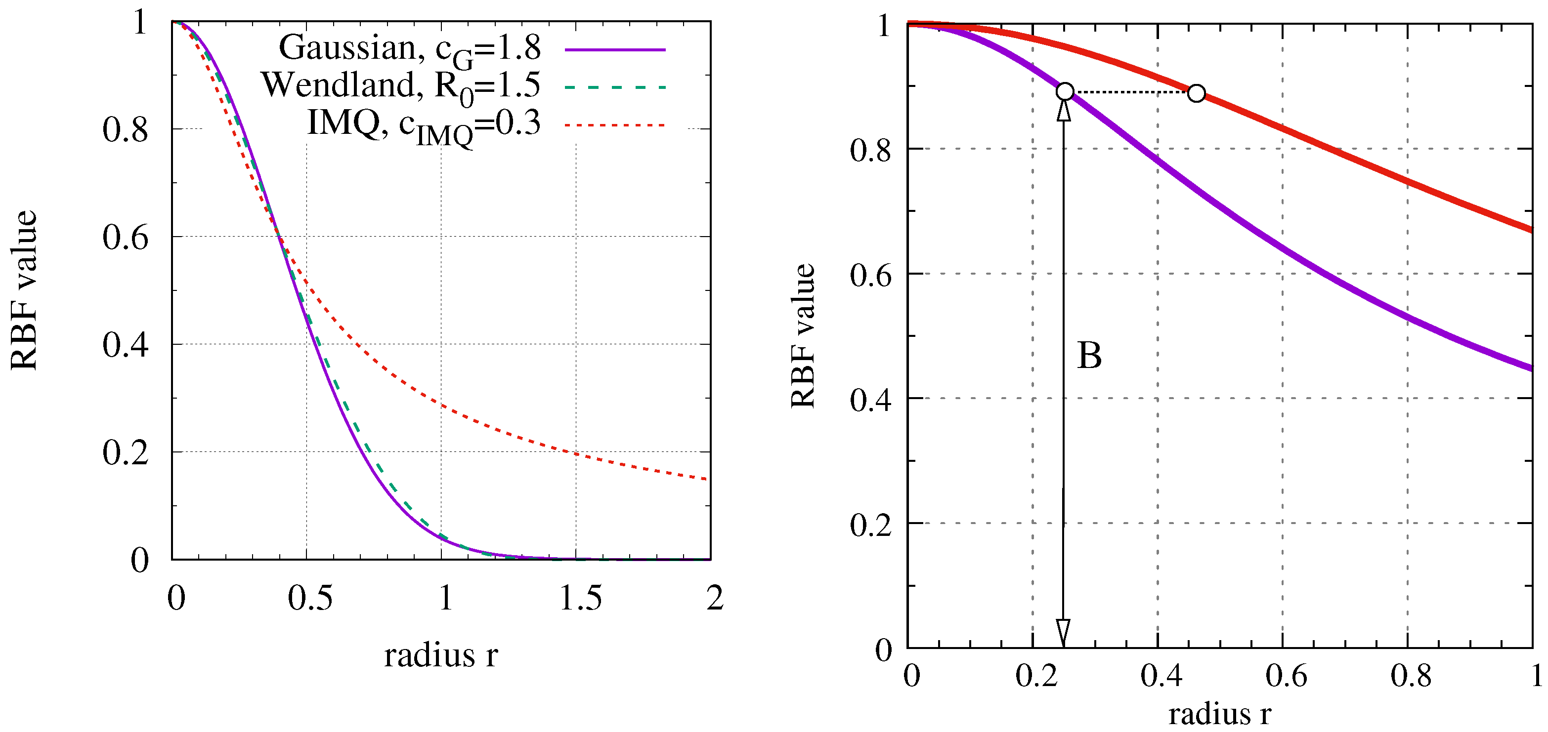
2.2. Radial Basis Functions

There are a number of approaches that use RBFs, see [7,8], mainly concerned with computer graphics, geometrical reconstruction, interpolation, and smoothing. Here, RBFs are applied to describe the motion of material surfaces, and the properties of surface deformations are evaluated, i.e., the stretch or strain determination.

Since a Cartesian basis is chosen in the following, it is possible to use column vectors $\mathbf{x}{\in \mathbb{R}}^3$ instead of geometrical vectors $\overrightarrow{x}\in {\mathbb{V}}^3$. Thus, a consistent matrix notation can be followed. The ansatz for the motion reads

$$\widehat{\mathbf{x}}(\mathsf{\Theta },t_n)=\sum _{j=1}^3\left(\sum _{k=1}^{n_{\mathrm{cp}}}\widehat{m}\left(\widehat{\rho }(\mathsf{\Theta },{\mathsf{\Theta }}_k)\right)B_{kj}^{\left(n\right)}+\sum _{l=1}^3{\widehat{n}}_l\left(\mathsf{\Theta }\right)D_{lj}^{\left(n\right)}\right){\mathbf{e}}_j$$

(13)

with

$$\widehat{\mathbf{n}}\left(\mathsf{\Theta }\right)=\left\{\begin{array}{c}{\widehat{n}}_1\left(\mathsf{\Theta }\right)\\ {\widehat{n}}_2\left(\mathsf{\Theta }\right)\\ {\widehat{n}}_3\left(\mathsf{\Theta }\right)\end{array}\right\}=\left\{\begin{array}{c}1\\ {\mathsf{\Theta }}^1\\ {\mathsf{\Theta }}^2\end{array}\right\}.$$

(14)

where the first part represents the RBF contribution and the second lower order polynomial part is chosen to fit rigid body motions and linear displacement fields. Here, ${\mathbf{e}}_j{\in \mathbb{R}}^3$, $j=1,2,3$, are column vectors—with a value 1 at the j-th entry and a value of zero at all other entries. $\mathsf{\Theta }{\in \mathbb{R}}^2$ with $\mathsf{\Theta }=\{{\mathsf{\Theta }}^1,{\mathsf{\Theta }}^2\}$ are the surface parameters of Section 2.1, where the simplest approach is to take the Cartesian coordinates in the initial configuration provided by the DIC-system, $({\mathsf{\Theta }}^1,{\mathsf{\Theta }}^2)=(X,Y)$.

$${\rho }_k=\widehat{\rho }(\mathsf{\Theta },{\mathsf{\Theta }}_k)=\frac{R}{R_0}=\frac{\parallel \mathsf{\Theta }-{\mathsf{\Theta }}_k\parallel }{R_0}=\frac{\sqrt{{(X-X_k)}^2+{(Y-Y_k)}^2}}{R_0}$$

(15)

defines the normalized distance function evaluated at the so-called center (or source) points ${\mathsf{\Theta }}_k=\{{\mathsf{\Theta }}_k^1,{\mathsf{\Theta }}_k^2\}=\{X_k^{\mathrm{cp}},Y_k^{\mathrm{cp}}\}$, $k=1,\dots ,n_{\mathrm{cp}}$, which might be equidistant points in the $(X,Y)$-space. $R_0$ is a radius for normalizing the RBFs, and $n_{\mathrm{cp}}$ are the number of center points. The coefficients $B_{kj}^{\left(n\right)}$ and $D_{lj}^{\left(n\right)}$ are the unknown weights.

The chosen radial basis functions $\widehat{m}\left(\rho \right)$ are depicted in

Table 1. Applied radial basis functions (here, expression $\langle a\rangle$ defines the Macaulay-brackets, $\langle a\rangle =a$ for $a>0$ and $\langle a\rangle =0$ for $a\le 0$).

		$\widehat{\mathit{m}}\left(\mathit{\rho }\right)$	${\widehat{\mathit{m}}}^{\prime }\left(\mathit{\rho }\right)$
Gaussian	${\widehat{m}}_G\left(\rho \right)$	${\displaystyle e^{-{\left(c_G\rho \right)}^2}}$	${\displaystyle -2c_G^2\rho e^{-{\left(c_G\rho \right)}^2}}$
Wendland [20]	${\widehat{m}}_W\left(\rho \right)$	${\displaystyle {\langle 1-\rho \rangle }^4(1+4\rho )}$	${\displaystyle -20\rho {\langle 1-\rho \rangle }^3}$
Inverse Multi-Quadrics	${\widehat{m}}_I\left(\rho \right)$	$\frac{{\displaystyle c_I}}{{\displaystyle \sqrt{{\rho }^2+c_I^2}}}$	$-\frac{{\displaystyle \rho c_I}}{{\displaystyle {({\rho }^2+c_I^2)}^{3/2}}}$

, although there are many other possible functions, e.g., splines, see [19]. The transposed position vector at a point ${\mathsf{\Theta }}_i$, $i=1,\dots ,n_{\mathrm{D}}^{\left(n\right)}$ (where $n_{\mathrm{D}}^{\left(n\right)}$ symbolizes the number of evaluation points), is given by

$${\mathbf{x}}_i^{\left(n\right)T}={\widehat{\mathbf{x}}}^T({\mathsf{\Theta }}_i,t_n)={\mathbf{m}}_i^T{\mathit{\kappa }}_R^{\left(n\right)}+{\mathbf{n}}_i^T{\mathit{\kappa }}_M^{\left(n\right)}={\mathbf{a}}_i^T{\mathit{\kappa }}^{\left(n\right)}.$$

(16)

Here, the vectors of evaluated radial basis functions and monomials are symbolized by

$$\begin{array}{cc}\hfill {\mathbf{m}}_i^T& =\{m_{i1}{m}_{i2}\dots m_{i{n}_{\mathrm{cp}}}\},m_{ik}=\widehat{m}\left(\widehat{\rho }({\mathsf{\Theta }}_i,{\mathsf{\Theta }}_k)\right),{\mathbf{m}}_i{\in \mathbb{R}}^{n_{\mathrm{cp}}}\hfill \end{array}$$

(17)

$$\begin{array}{cc}\hfill {\mathbf{n}}_i^T& =\left\{1X_i{Y}_i\right\},{\mathbf{n}}_i=\widehat{\mathbf{n}}\left({\mathsf{\Theta }}_i\right),{\mathbf{n}}_i{\in \mathbb{R}}^3\hfill \end{array}$$

(18)

$$\begin{array}{cc}\hfill {\mathbf{a}}_i^T& =\left\{{\mathbf{m}}_i^T{\mathbf{n}}_i^T\right\},{\mathbf{a}}_i{\in \mathbb{R}}^{n_{\mathrm{cp}}+3},\hfill \end{array}$$

(19)

$i=1,\dots ,n_{\mathrm{D}}^{\left(n\right)}$, $k=1,\dots ,n_{\mathrm{cp}}$, and the matrices of unknowns by

$${\mathit{\kappa }}_R^{\left(n\right)}=\left[\begin{array}{ccc}{B}_{11}^{\left(n\right)}& B_{12}^{\left(n\right)}& B_{13}^{\left(n\right)}\\ ⋮& ⋮& ⋮\\ B_{n_{\mathrm{cp}}1}^{\left(n\right)}& B_{n_{\mathrm{cp}}2}^{\left(n\right)}& B_{n_{\mathrm{cp}}3}^{\left(n\right)}\end{array}\right],{\mathit{\kappa }}_M^{\left(n\right)}=\left[\begin{array}{ccc}{D}_{11}^{\left(n\right)}& D_{12}^{\left(n\right)}& D_{13}^{\left(n\right)}\\ D_{21}^{\left(n\right)}& D_{22}^{\left(n\right)}& D_{23}^{\left(n\right)}\\ D_{31}^{\left(n\right)}& D_{32}^{\left(n\right)}& D_{33}^{\left(n\right)}\end{array}\right],{\mathit{\kappa }}^{\left(n\right)}=\left[\begin{array}{c}{\mathit{\kappa }}_R^{\left(n\right)}\\ {\mathit{\kappa }}_M^{\left(n\right)}\end{array}\right],$$

(20)

${\mathit{\kappa }}^{\left(n\right)}{\in \mathbb{R}}^{(n_{\mathrm{cp}}+3)\times 3}$, ${\mathit{\kappa }}_R^{\left(n\right)}{\in \mathbb{R}}^{n_{\mathrm{cp}}\times 3}$, ${\mathit{\kappa }}_M^{\left(n\right)}{\in \mathbb{R}}^{3\times 3}$, at each evaluation time $t_n$ (the superscript T symbolizes the transposition). The residual between the simulation (model) ${\mathbf{r}}_i^{\left(n\right)}$ and the experimental data ${\mathbf{d}}_i^{\left(n\right)}$ at that point

$${\mathbf{r}}_i^{\left(n\right)T}={\mathbf{x}}_i^{\left(n\right)T}-{\mathbf{d}}_i^{\left(n\right)T}={\mathbf{a}}_i^T{\mathit{\kappa }}^{\left(n\right)}-{\mathbf{d}}_i^{\left(n\right)T}$$

(21)

is required either for interpolation or for regression using a linear least-square approach to determine the unknown parameters ${\mathit{\kappa }}^{\left(n\right)}$. If all residuals are assembled, the matrix of residuals

$$\underset{{\mathbf{R}}^{\left(n\right)}}{\underbrace{\left[\begin{array}{c}{\mathbf{r}}_1^{\left(n\right)T}\\ ⋮\\ {\mathbf{r}}_{n_{\mathrm{D}}^{\left(n\right)}}^{\left(n\right)T}\end{array}\right]}}=\underset{{\mathbf{A}}^{\left(n\right)}}{\underbrace{\left[\begin{array}{c}{\mathbf{a}}_1^T\\ ⋮\\ {\mathbf{a}}_{n_{\mathrm{D}}^{\left(n\right)}}^T\end{array}\right]}}{\mathit{\kappa }}^{\left(n\right)}-\underset{{\mathbf{D}}^{\left(n\right)}}{\underbrace{\left[\begin{array}{c}{\mathbf{d}}_1^{\left(n\right)T}\\ ⋮\\ {\mathbf{d}}_{n_{\mathrm{D}}^{\left(n\right)}}^{\left(n\right)T}\end{array}\right]}}$$

(22)

with ${\mathbf{R}}^{\left(n\right)}{\in \mathbb{R}}^{n_{\mathrm{D}}^{\left(n\right)}\times 3}$, ${\mathbf{A}}^{\left(n\right)}{\in \mathbb{R}}^{n_{\mathrm{D}}^{\left(n\right)}\times (n_{\mathrm{cp}}+3)}$, ${\mathbf{\kappa }}^{\left(n\right)}{\in \mathbb{R}}^{(n_{\mathrm{cp}}+3)\times 3}$, and ${\mathbf{D}}^{\left(n\right)}{\in \mathbb{R}}^{n_{\mathrm{D}}^{\left(n\right)}\times 3}$ is obtained.

In principle, there are three basic possibilities to determine the unknowns ${\mathbf{\kappa }}^{\left(n\right)}$:

Interpolation: First, it is assumed that the center points ${\mathsf{\Theta }}_k$ are equivalent to the evaluation (data) points ${\mathsf{\Theta }}_i$, i.e., $n_{\mathrm{cp}}=n_{\mathrm{D}}^{\left(n\right)}$, and that there are no additional monomials. Then, the residual (22) is zero, ${\mathrm{R}}^{\left(n\right)}=0$, and degenerates to the system of linear equations with three right-hand sides,

$${\mathbf{A}}^{\left(n\right)}{\mathbf{\kappa }}_R^{\left(n\right)}={\mathbf{D}}^{\left(n\right)}$$

(23)

with ${\mathbf{a}}_i={\mathbf{m}}_i$, $i=1,\dots ,n_{\mathrm{D}}^{\left(n\right)}$. If monomials are used in addition to RBFs and the center points are identical to the data points, more unknowns than equations occur. Here, it is common to assume the orthogonality conditions

$$\sum _{k=1}^{n_{\mathrm{D}}^{\left(n\right)}}{B}_{kj}^{\left(n\right)}{\mathbf{n}}_k=\mathbf{0}$$

(24)

leading to the linear system

$${\mathbf{A}}^{\left(n\right)}{\mathbf{\kappa }}^{\left(n\right)}=\left[\begin{array}{c}{\mathbf{D}}^{\left(n\right)}\\ {\mathbf{0}}_{(3\times 3)}\end{array}\right]\mathrm{with}{\mathbf{A}}^{\left(n\right)}=\left[\begin{array}{cc}{\mathbf{m}}_1^T& {\mathbf{n}}_1^T\\ ⋮& ⋮\\ {\mathbf{m}}_{n_{\mathrm{D}}^{\left(n\right)}}^T& {\mathbf{n}}_{n_{\mathrm{D}}^{\left(n\right)}}^T\\ {\mathbf{n}}_1\dots {\mathbf{n}}_{n_{\mathrm{D}}^{\left(n\right)}}& {\mathbf{0}}_{(3\times 3)}\end{array}\right].$$

(25)

Regression: If it is not assumed that the data (evaluation) points are identical to the center points, a linear least-square problem can be formulated (under the condition $n_{\mathrm{cp}}\le n_{\mathrm{D}}^{\left(n\right)}-3$). The least-square problem requires that the square of residuals should be a minimum,

$$f\left({\mathbf{\kappa }}^{\left(n\right)}\right)=\frac{1}{2}{\mathbf{R}}^{\left(n\right)}\left({\mathbf{\kappa }}^{\left(n\right)}\right)·{\mathbf{R}}^{\left(n\right)}\left({\mathbf{\kappa }}^{\left(n\right)}\right)\to \min .$$

(26)

yielding the system of linear equations with several right-hand sides

$$\left[{\mathbf{A}}^{\left(n\right)T}{\mathbf{A}}^{\left(n\right)}\right]{\mathbf{\kappa }}^{\left(n\right)}={\mathbf{A}}^{\left(n\right)T}{\mathbf{D}}^{\left(n\right)}$$

(27)

to determine the unknown parameters ${\mathbf{\kappa }}^{\left(n\right)}$ (the inner product in Equation (26) is defined for an arbitrary matrix $\mathbf{K}{\in \mathbb{R}}^{m\times n}$ by $\mathbf{K}·\mathbf{K}={\sum }_{i=1}^m{\sum }_{j=1}^n{K}_{ij}{K}_{ij}$). It should also be noted that ${\mathsf{\Theta }}_i^T=\left\{d_{i1}^{\left(n\right)}{d}_{i2}^{\left(n\right)}\right\}$, i.e., the $(X_i,Y_i)$-coordinates of the data vectors are chosen in Equation (16) in our applications later on.

Various solution schemes can be applied to the linear systems (23), (25) or (27) (direct vs. iterative solvers, solvers for sparse matrices applicable for, e.g., the Wendland function or the Gaussian function if a truncation of values close to zero is applied, singular value decomposition for very ill-conditioned systems, fast solvers, …, see, for example [8,12,21,22] and the literature cited therein). In this rather introductory paper, we confine our attention to the principle properties of the entire approach to strain determination in full-field strain measurements.

2.3. Application of Radial Basis Functions for Strain Determination

To determine the principal stretches (or strains), the tangent vectors ${\overrightarrow{a}}_{\alpha }=\partial \widehat{\overrightarrow{x}}/\partial {\mathsf{\Theta }}^{\alpha }$ are needed in Equation (1), i.e.,

$${\mathbf{a}}_{\alpha }^{\left(n\right)}=\frac{{\displaystyle \partial \widehat{\mathbf{x}}(\mathsf{\Theta },t_n)}}{{\displaystyle \partial {\mathsf{\Theta }}^{\alpha }}}=\sum _{j=1}^3\left(\sum _{k=1}^{n_{\mathrm{cp}}}\frac{{\displaystyle \mathrm{d}\widehat{m}}}{{\displaystyle \mathrm{d}\rho }}\frac{{\displaystyle \partial {\widehat{\rho }}_k}}{{\displaystyle \partial {\mathsf{\Theta }}^{\alpha }}}{B}_{kj}^{\left(n\right)}+\sum _{l=1}^3\frac{{\displaystyle \partial {\widehat{n}}_l}}{{\displaystyle \partial {\mathsf{\Theta }}^{\alpha }}}{D}_{lj}^{\left(n\right)}\right){\mathbf{e}}_j,{\mathbf{a}}_{\alpha }^{\left(n\right)}{\in \mathbb{R}}^3.$$

(28)

The derivatives ${\widehat{m}}^{\prime }\left(\rho \right)$ are compiled in Table 1, and

$$\frac{{\displaystyle \partial {\widehat{\rho }}_k}}{{\displaystyle \partial {\mathsf{\Theta }}^{\alpha }}}=\frac{{\mathsf{\Theta }}^{\alpha }-{\mathsf{\Theta }}_k^{\alpha }}{\parallel \mathsf{\Theta }-{\mathsf{\Theta }}_k\parallel }.$$

(29)

For the initial state, this reads

$${\mathbf{A}}_{\alpha }={\mathbf{a}}_{\alpha }^{\left(0\right)}=\sum _{j=1}^3\left(\sum _{k=1}^{n_{\mathrm{cp}}}\frac{{\displaystyle \mathrm{d}\widehat{m}}}{{\displaystyle \mathrm{d}\rho }}\frac{{\displaystyle \partial {\widehat{\rho }}_k}}{{\displaystyle \partial {\mathsf{\Theta }}^{\alpha }}}{B}_{kj}^{\left(0\right)}+\sum _{l=1}^3\frac{{\displaystyle \partial {\widehat{n}}_l}}{{\displaystyle \partial {\mathsf{\Theta }}^{\alpha }}}{D}_{lj}^{\left(0\right)}\right){\mathbf{e}}_j,{\mathbf{A}}_{\alpha }{\in \mathbb{R}}^3$$

(30)

which is required for the matrix of metric coefficients, $A_{\alpha \beta }={\mathbf{A}}_{\alpha }^T{\mathbf{A}}_{\beta }$, to calculate the gradient vectors ${\mathbf{A}}^{\alpha }$. This allows the calculation of the deformation gradient (1) and, accordingly, the principal stretches (10).

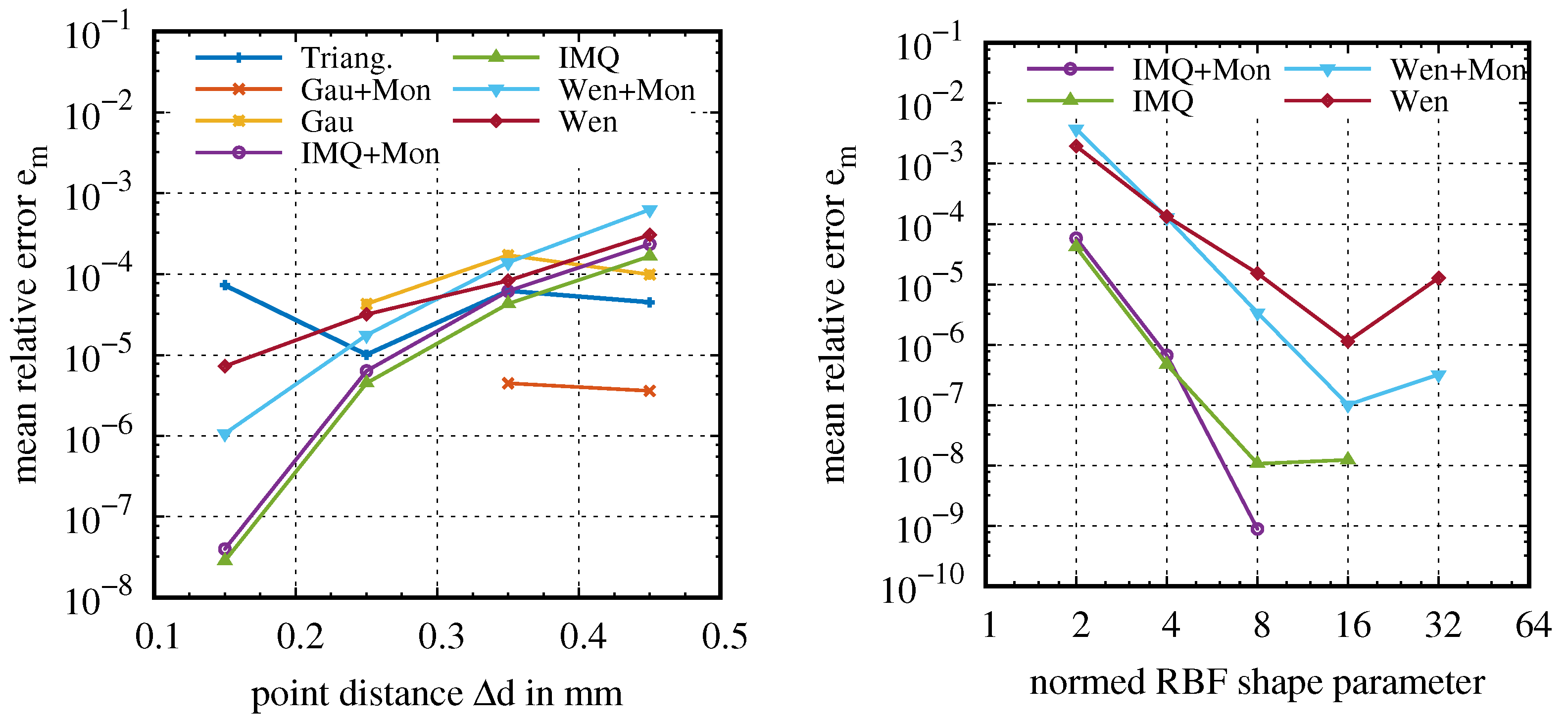
3. Evaluation of Strain Determination Using RBFs

In the following subsections, the behavior of the full-field strain measurement using radial basis functions is investigated. For this purpose, the basic properties of the approach is studied first using verification examples for which analytical solutions are known. Next, the concept is applied to real experimental data obtained from WAAM-produced specimens.

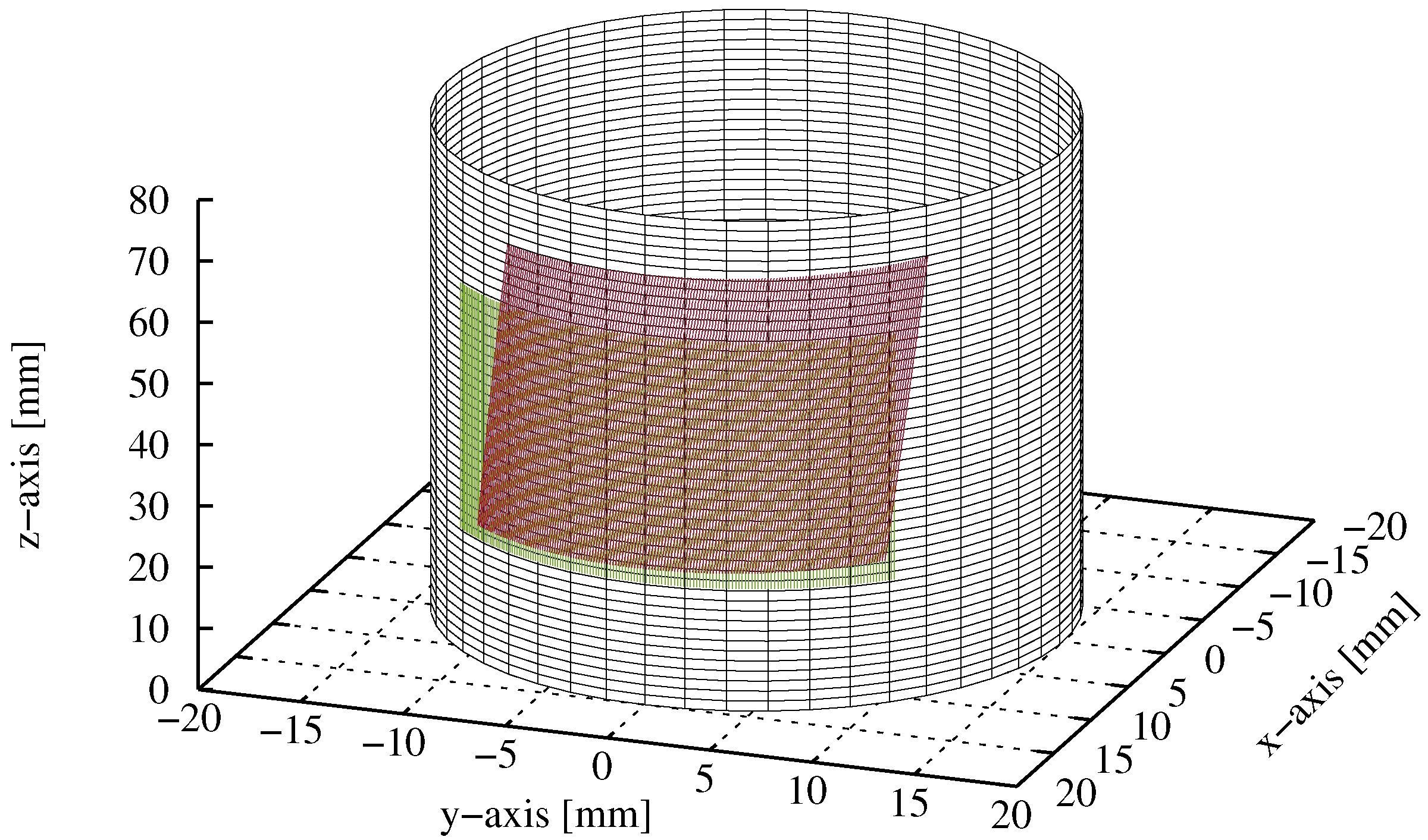
3.1. Verification Examples of WAAM-Produced Cylindrical Components

We are interested in comparing the properties of the RBF-approach with the classical triangulation concept. For this purpose, an analytical example of a surface deformation is considered, which is similar to a real sample produced by a WAAM-process. In a first step, however, pure tension and torsion of a cylindrical tube with a smooth surface is considered so that the order of possible additional errors due to the roughness of the specimens can be interpreted in the subsequent step.

3.1.1. Tension and Torsion of a Cylindrical Tube

To study the accuracy of the new approach using RBFs, the analytic deformation of tension and torsion is compared to the numerical results. For more details on the analytical equations and their derivation, refer to [23,24,25,26], and with an application to DIC, to [4]. Here, the motion

$$\overrightarrow{x}={\overrightarrow{\chi }}_{\mathrm{R}}(\overrightarrow{X},t)=\widehat{r}\left(R\right){\overrightarrow{e}}_r(\mathsf{\Phi },Z)+\widehat{z}\left(Z\right){\overrightarrow{e}}_z$$

(31)

is considered, with

$$\widehat{r}\left(R\right)={\lambda }^{-1/2}R,\widehat{\phi }(\mathsf{\Phi },Z)=\mathsf{\Phi }+DZ,\widehat{z}\left(Z\right)=\lambda Z,$$

(32)

and

$${\overrightarrow{e}}_r=cos\phi {\overrightarrow{e}}_x+sin\phi {\overrightarrow{e}}_y,{\overrightarrow{e}}_{\phi }=-sin\phi {\overrightarrow{e}}_x+cos\phi {\overrightarrow{e}}_y.$$

(33)

$\lambda =L/L_0$ defines the axial stretch, where L is the current length and $L_0$ the initial length of the cylinder. $D=\alpha /L_0$ symbolizes the twist, where $\alpha$ represents the torsion angle. The motion (31) yields the principal stretches

$${\lambda }_1={\lambda }^{-1/2},{\lambda }_{2,3}=\sqrt{\frac{1+{\lambda }^3+{\left(DR\right)}^2\pm \sqrt{{(1+{\lambda }^3+{\left(DR\right)}^2)}^2-4{\lambda }^3}}{2\lambda }},$$

(34)

representing the eigenvalues of the right stretch tensor $\mathbf{U}$ of the polar decomposition $\mathbf{F}=\mathbf{R}\mathbf{U}$, where $\mathbf{F}(\overrightarrow{X},t)=Grad{\overrightarrow{\chi }}_{\mathrm{R}}(\overrightarrow{X},t)$ defines the deformation gradient, and $\mathbf{R}$ with $det\mathbf{R}=+1$, ${\mathbf{R}}^T={\mathbf{R}}^{-1}$, the rotation tensor.

In the following example, a fixed radius $R=15\mathrm{mm}$, $L_0=80\mathrm{mm}$, $\lambda =1.2$, and a torsional angle of $\alpha =20{}^{\circ }$ are assumed, so that $D=\alpha /L_0=20{}^{\circ }\pi /180{}^{\circ }/80\mathrm{mm}\approx 0.44{\mathrm{mm}}^{-1}$. See Figure 1 for the points on the surface in the reference and the current configuration. The analytical solution yields the stretches

$${\lambda }_1=0.91287,{\lambda }_2=1.2035,{\lambda }_3=0.91022.$$

(35)

We are interested in the in-plane stretches ${\lambda }_2$ and ${\lambda }_3$, which can be compared to the DIC-results. ${\lambda }_1$ defines the out-of-plane component, which cannot be measured. The maximum principal stretch is ${\lambda }_2$ ($(+)$-sign in Equation (34)${}_2$).

For the numerically generated DIC-data, a center region ($\mathsf{\Phi }\in [-45{}^{\circ },+45{}^{\circ }]$, $Z\in [20\mathrm{m}\mathrm{m},60\mathrm{m}\mathrm{m}]$) is assumed. Then, equidistant points are generated using Equation (31) for constant R with a distance $\mathsf{\Delta }d$ in each $\mathsf{\Phi }$- and Z-direction. In a first investigation, the pointwise relative error of the maximum principal stretch of the RBF-approach relative to the analytical (exact) stretch ${\lambda }_{\mathrm{ex}}={\lambda }_2$ in Equation (35)

$$e_{{\lambda }_k}=\frac{|{\lambda }_k^{\mathrm{DIC}}-{\lambda }_{\mathrm{ex}}|}{{\lambda }_{\mathrm{ex}}}\times 100,$$

(36)

is defined. Here, $\mathsf{\Delta }d=0.15\mathrm{m}\mathrm{m}$ is chosen. Further, the Wendland function ${\widehat{m}}_W\left(\rho \right)$ combined with the linear polynomial (monomials), see Table 1, with $R_0=1.5\mathrm{m}\mathrm{m}$ is applied to visualize the boundary effects, see Figure 2.

Although the points are fulfilled exactly, the derivatives—here represented by the stretches—show larger errors at the boundary of the evaluation region, which is one of the weaknesses of the RBF-method that were found in the scope of the study. This will be considered in the following investigation.

In the following figures, the mean value of all errors is calculated

$$e_m=\frac{{\displaystyle 1}}{{\displaystyle n^{\mathrm{DIC}}}}\sum _{k=1}^{n^{\mathrm{DIC}}}{e}_{{\lambda }_k},$$

(37)

in a region of interest. $n^{\mathrm{DIC}}$ is the number of data points considered. Since there is the boundary effect of the RBF, see Figure 2, the following evaluations will only consider points in the region $-25{}^{\circ }\le \mathsf{\Phi }\le 25{}^{\circ }$, $30\mathrm{m}\mathrm{m}\le Z\le 50\mathrm{m}\mathrm{m}$.

Remark 1.

The region of interest is chosen in an arbitrary manner to circumvent the influence of the individual shape parameters of each RBF, and to avoid the boundary effects that lead to a further misrepresentation of the convergence behavior. Not only the RBFs show such boundary effects. On a closer look at the triangulation concept, all triangles are omitted which have angles below a permissible critical angle. This serves to also exclude highly inaccurate solutions that occur due to the coordinate transformation between global and surface coordinates. To circumvent this discussion for both approaches, we restrict ourselves to the seemingly arbitrary center region.

To compare the new approach, the classical triangulation concept is considered as well. Here, geometry and deformation are interpolated with shape functions for triangles, similar to the finite element method. The triangulation is completed with the method of [27,28]. Within each triangle, the in-plane stretches (or for practical applications the principal in-plane strains, can be determined, see [4]). This is followed by a calculation of the mean value of the principal stretches of triangles adjacent to a data point (this implies an additional interpolation). For our investigations, the point distance $\mathsf{\Delta }d=\{0.15,0.25,0.35,0.45\}$ is varied and the mean relative error (37) of the different methods is analyzed, see Figure 3 (left).

To allow for a comparison of the functions ${\widehat{m}}_G\left(\rho \right)$, ${\widehat{m}}_W\left(\rho \right)$, and ${\widehat{m}}_I\left(\rho \right)$, the shape factors are chosen to be constant, but in such a manner that the functions look quite similar ($R_0=1.5\mathrm{m}\mathrm{m}$, $c_G=2.7$, $c_I=0.2$), see Appendix A. The Gaussian-RBF ${\widehat{m}}_G\left(\rho \right)$ with monomials (Gau + Mon) show very good results in comparison to the triangulation concept. However, the condition number of the resulting systems of linear Equations (23) and (25) are too large for particular point distances so that the systems are not solvable for smaller values of the point distances $\mathsf{\Delta }d$, see

Table 2. Order of condition numbers of the linear systems for different interpolation schemes and varying point distance ($R_0=1.5\mathrm{m}\mathrm{m}$, $c_G=2.7$, $c_I=0.2$). Here, the expert driver routines of [29] are chosen.

$\mathsf{\Delta }\mathit{d}$	Gau	Gau + Mon	Wen	Wen + Mon	IMQ	IMQ + Mon
0.15	${10}^{29}$	${10}^{34}$	${10}^4$	${10}^9$	${10}^6$	${10}^9$
0.25	${10}^{12}$	${10}^{16}$	${10}^3$	${10}^8$	${10}^4$	${10}^7$
0.35	${10}^6$	${10}^{10}$	${10}^2$	${10}^7$	${10}^3$	${10}^6$
0.45	${10}^3$	${10}^8$	${10}^2$	${10}^6$	${10}^3$	${10}^6$

.

Thus, the relation between the point distance and the shape factor $c_G$ is essential—as it is known from the literature. The Wendland function ${\widehat{m}}_W\left(\rho \right)$ shows much better properties. Since there is an intersection of the pure RBF approach (Wen) with the extension of monomials (Wen + Mon), there cannot be made an accuracy statement whether linear polynomials are essential. Looking only at the condition numbers, the consideration of monomials increases the condition numbers again. The inverse multi-quadrics approach (IMQ) and (IMQ + Mon) yields similar results regarding the aspect of conditioning but better results in the accuracy. The latter can be interpreted by the course of the function, see Figure A1, which shows a larger region until the values of the function becomes very small. Thus, linear functions seem to be better approximated—leading to the property that the monomial approach implies more linear dependencies of the column vectors in the linear system.

In the next study, the point distance is fixed by $\mathsf{\Delta }d=0.25\mathrm{m}\mathrm{m}$. Then, the normalized shape factor ${\beta }_W=R_0/\mathsf{\Delta }d=R_0/0.25$ and that of the inverse multi-quadrics function, $c_{\mathrm{IMQ}}:=c_I{R}_0={\beta }_I/10$, are varied, see Figure 3 (right). The factor $1/10$ is chosen for a better presentation in Figure 3 (right). The inverse multi-quadrics converges very fast for increasing shape factor ${\beta }_I$. However, only solutions for particular linear systems due to exceeding condition numbers for ${\beta }_I<8$ (IMQ) and ${\beta }_I<16$ (IMQ + Mon) are obtained.

A possible approach of estimating the shape factor ${\widehat{c}}_{\mathrm{IMQ}}\left(\mathsf{\Delta }d\right)$—in dependence of the point distance $\mathsf{\Delta }d$ so that accuracy and condition number are appropriate—is provided in Appendix A.

The advantage of having only one function representing the deformation offers the simple possibility to evaluate—apart from the principal stretches or strains—the principal direction concerned. Here, two possibilities can be considered, see [4], either the eigenvectors of the in-plane right stretch tensor $\widehat{\mathbf{U}}$ or the in-plane left stretch tensor $\widehat{\mathbf{V}}$. The in-plane left stretch tensor stems from the polar decomposition $\widehat{\mathbf{F}}=\widehat{\mathbf{V}}\widehat{\mathbf{R}}$ and can be determined either by the eigenvalue problem of the left Cauchy-Green tensor $\widehat{\mathbf{B}}=\widehat{\mathbf{F}}{\widehat{\mathbf{F}}}^T={\widehat{\mathbf{V}}}^2$ or by rotating the eigenvectors of the in-plane right stretch tensor $\widehat{\mathbf{U}}$ by the rotation tensor $\widehat{\mathbf{R}}$. The latter is omitted for brevity. Figure 4 shows the distribution of the principal direction (eigenvectors) of the in-plane right stretch tensor $\widehat{\mathbf{U}}$ evaluated at particular positions on the sample’s surface. Both possibilities are commonly not provided in DIC-evaluation programs, or are not explained in a thorough manner. However, these principal directions might provide a sound interpretation of the load distribution in the presence of inhomogeneous deformations. Thus, Figure 4 shows the known principal directions for the “simple” problem of tension and torsion, where the RBF-results are evaluated.

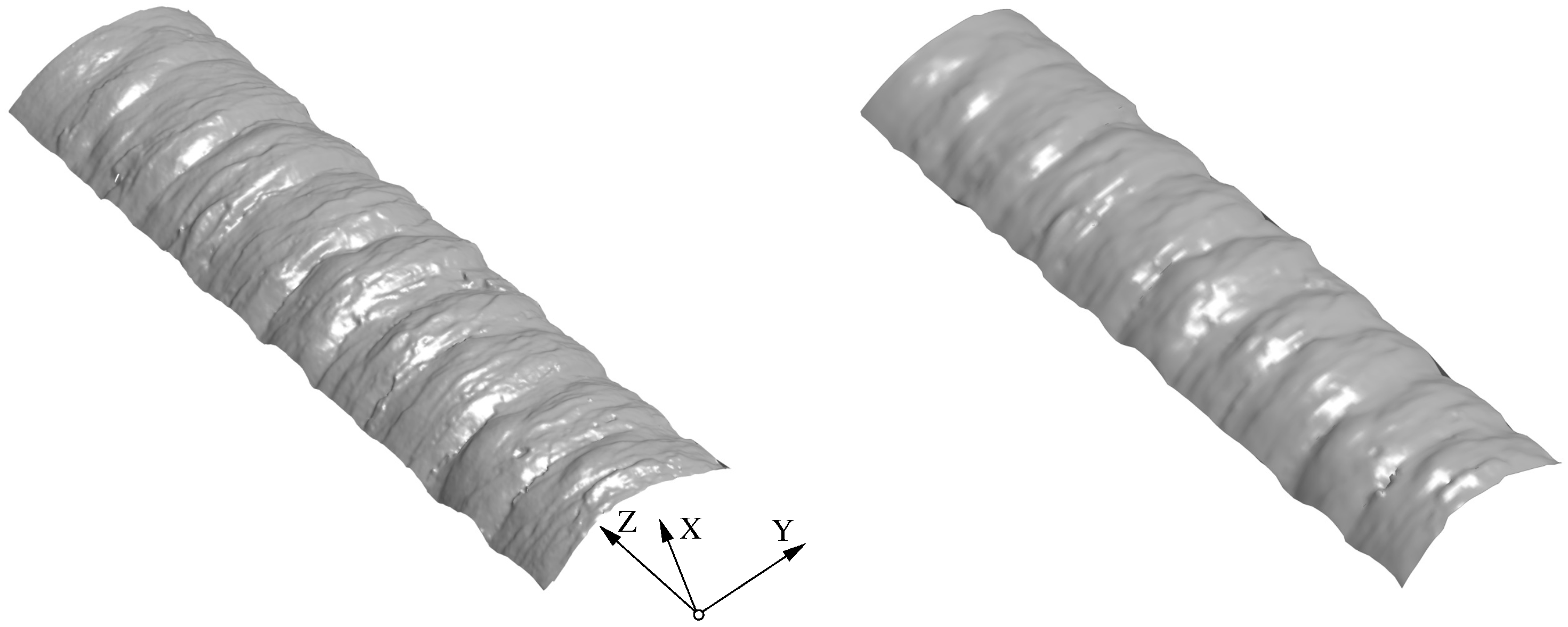
3.1.2. Tension and Torsion of a Tube with Rough Surface

With WAAM components that have already been manufactured, the actual objective is that the surfaces, see Figure 5 (right), as an example, are not treated any more. This poses further challenges to image correlation methods, since—although classical paints and spray-on speckle patterns can be used—the surfaces have a high degree of roughness. The strains on the surfaces, on the other hand, are difficult to evaluate because the interpolations smooth out the local features. To investigate this, it is possible to use a verification example of the following type: a cylindrical specimen with a rough surface in the initial configuration is considered

$$\overrightarrow{X}({\mathsf{\Theta }}^1,{\mathsf{\Theta }}^2)=\overrightarrow{X}(\mathsf{\Phi },Z)=\widehat{R}\left(Z\right){\overrightarrow{E}}_R\left(\mathsf{\Phi }\right)+Z{\overrightarrow{E}}_Z,$$

(38)

where $({\mathsf{\Theta }}^1,{\mathsf{\Theta }}^2)=(\mathsf{\Phi },Z)$ are the curvilinear coordinates, and ${\overrightarrow{E}}_R\left(\mathsf{\Phi }\right)=cos\mathsf{\Phi }{\overrightarrow{e}}_x+sin\mathsf{\Phi }{\overrightarrow{e}}_y$, and ${\overrightarrow{E}}_{\mathsf{\Phi }}\left(\mathsf{\Phi }\right)=-sin\mathsf{\Phi }{\overrightarrow{e}}_x+cos\mathsf{\Phi }{\overrightarrow{e}}_y$, the radial and circumferential directions. First, a smoothed step-function for the varying radius describing the welding bead stacks is applied,

$$\begin{array}{cc}\hfill \tilde{R}\left(Z\right)& =R_0+\frac{D_S}{2}\sum _{k=0}^{n_{\mathrm{ws}}}\left(tanh\left(c(Z-(Z_k+\delta ))\right)-tanh\left(c(Z-(Z_{k+1}-\delta ))\right)\right),\hfill \end{array}$$

(39)

$$\begin{array}{cc}\hfill Z_k& =Z_0+kH.\hfill \end{array}$$

(40)

$R_0$ is the mean radius of the tube, $D_S$ controls the notch depth between two stacks of welding beads, and $n_{\mathrm{ws}}$ defines the number of stacks over the specimen’s height. Here, one can only describe a pause by the welding robot, which has to stop after a certain number of welding beads to guarantee sufficient heat transport (The welding robot must be stopped after a few cycles of material application, as poor heat transfer causes the material to become too viscous and the specimens tend to melt away. The stopping time is necessary so that solidification is guaranteed). These welding layers build a welding stack of height H. Here, $\delta \ll H$ is chosen for a certain notch width between the step functions describing the stacks, and c (dimension: 1/length) serves to sharpen the notch, see Figure 6.

The individual welding layers (welding beads) are then described with the aid of a superposition of sinusoidal functions,

$$\widehat{R}\left(Z\right)=\tilde{R}\left(Z\right)+\frac{D_W}{2}\left(1+sin\left(\frac{2\pi n_{\mathrm{wb}}}{H}Z\right)\right),$$

(41)

where $n_{\mathrm{wb}}$ represents the number of welding beads within one stack of height H.

Next, the deformation

$$\overrightarrow{x}={\overrightarrow{\chi }}_{\mathrm{R}}(\overrightarrow{X},t)=\widehat{r}\left(R\right){\overrightarrow{e}}_r\left(\phi \right)+\widehat{z}\left(Z\right){\overrightarrow{e}}_z,$$

(42)

is assumed, where the radial motion depends only on Z, $\overline{r}\left(Z\right)=\widehat{r}\left(\widehat{R}\left(Z\right)\right)$, see Equation (41). Furthermore, $\phi =\mathsf{\Phi }+DZ$ holds for torsional problems, see Equation (32)${}_2$, which leads to

$$\begin{array}{cc}\hfill {\overrightarrow{e}}_r(\mathsf{\Phi },Z)& =cos\left(DZ\right){\overrightarrow{E}}_R\left(\mathsf{\Phi }\right)+sin\left(DZ\right){\overrightarrow{E}}_{\mathsf{\Phi }}\left(\mathsf{\Phi }\right)\hfill \\ \hfill {\overrightarrow{e}}_{\phi }(\mathsf{\Phi },Z)& =-sin\left(DZ\right){\overrightarrow{E}}_R\left(\mathsf{\Phi }\right)+cos\left(DZ\right){\overrightarrow{E}}_{\mathsf{\Phi }}\left(\mathsf{\Phi }\right)\hfill \\ \hfill {\overrightarrow{e}}_z& ={\overrightarrow{E}}_Z.\hfill \end{array}$$

(43)

Inserting this basis into the motion (42) yields

$$\overrightarrow{x}={\overrightarrow{\chi }}_{\mathrm{R}}(\overrightarrow{X},t)=\overline{r}\left(Z\right)cos\left(DZ\right){\overrightarrow{E}}_R\left(\mathsf{\Phi }\right)+\overline{r}\left(Z\right)sin\left(DZ\right){\overrightarrow{E}}_{\mathsf{\Phi }}\left(\mathsf{\Phi }\right)+\widehat{z}\left(Z\right){\overrightarrow{E}}_Z.$$

(44)

The in-plane deformation gradient (1) requires the tangent vectors

$$\begin{array}{cc}\hfill {\overrightarrow{a}}_1& =\frac{{\displaystyle \partial \overrightarrow{x}}}{{\displaystyle \partial \mathsf{\Phi }}}={\widehat{a}}_R\left(Z\right){\overrightarrow{E}}_R\left(\mathsf{\Phi }\right)+{\widehat{a}}_{\mathsf{\Phi }}\left(Z\right){\overrightarrow{E}}_{\mathsf{\Phi }}\left(\mathsf{\Phi }\right)\hfill \end{array}$$

(45)

$$\begin{array}{cc}\hfill {\overrightarrow{a}}_2& =\frac{{\displaystyle \partial \overrightarrow{x}}}{{\displaystyle \partial Z}}={\widehat{b}}_R\left(Z\right){\overrightarrow{E}}_R\left(\mathsf{\Phi }\right)+{\widehat{b}}_{\mathsf{\Phi }}\left(Z\right){\overrightarrow{E}}_{\mathsf{\Phi }}\left(\mathsf{\Phi }\right)+{\widehat{b}}_Z\left(Z\right){\overrightarrow{E}}_Z\hfill \end{array}$$

(46)

with

$$\begin{array}{cccc}\hfill {\widehat{a}}_R\left(Z\right)& =-\overline{r}\left(Z\right)sin\left(DZ\right),\hfill & \hfill {\widehat{a}}_{\mathsf{\Phi }}\left(Z\right)& =\overline{r}\left(Z\right)cos\left(DZ\right),\hfill \end{array}$$

(47)

$$\begin{array}{cccc}\hfill {\widehat{b}}_R\left(Z\right)& ={\overline{r}}^{\prime }\left(Z\right)cos\left(DZ\right)-D\overline{r}\left(Z\right)sin\left(DZ\right),\hfill & \hfill {\widehat{b}}_{\mathsf{\Phi }}\left(Z\right)& ={\overline{r}}^{\prime }\left(Z\right)sin\left(DZ\right)+D\overline{r}\left(Z\right)cos\left(DZ\right),\hfill \end{array}$$

(48)

and ${\widehat{b}}_Z\left(Z\right)={\widehat{z}}^{\prime }\left(Z\right)$. When calculating the gradient vectors ${\overrightarrow{A}}^{\alpha }$, the tangent vectors

$${\overrightarrow{A}}_1=\frac{{\displaystyle \partial \overrightarrow{X}}}{{\displaystyle \partial \mathsf{\Phi }}}=\widehat{R}\left(Z\right){\overrightarrow{E}}_{\mathsf{\Phi }}\left(\mathsf{\Phi }\right),{\overrightarrow{A}}_2=\frac{{\displaystyle \partial \overrightarrow{X}}}{{\displaystyle \partial Z}}={\widehat{R}}^{\prime }\left(Z\right){\overrightarrow{E}}_R\left(\mathsf{\Phi }\right)+{\overrightarrow{E}}_Z$$

(49)

are required. Here, the property ${\overrightarrow{E}}_R^{\prime }\left(\mathsf{\Phi }\right)={\overrightarrow{E}}_{\mathsf{\Phi }}\left(\mathsf{\Phi }\right)$ is exploited (the prime means the derivative with respect to the argument of the function). The inverse of the matrix of covariant metric coefficients

$$\left[A_{\alpha \beta }\right]=\left[\begin{array}{cc}{\widehat{R}}^2\left(Z\right)& \\ & 1+{\widehat{R}}^{\prime 2}\left(Z\right)\end{array}\right]$$

(50)

i.e.,

$$\left[A^{\alpha \beta }\right]=\left[\begin{array}{cc}1/{\widehat{R}}^2\left(Z\right)& \\ & 1/(1+{\widehat{R}}^{\prime 2}\left(Z\right))\end{array}\right]$$

(51)

yields together with ${\overrightarrow{A}}^{\alpha }=A^{\alpha \beta }{\overrightarrow{A}}_{\beta }$ the contravariant vectors

$${\overrightarrow{A}}^1=\frac{{\displaystyle 1}}{{\displaystyle \widehat{R}\left(Z\right)}}{\overrightarrow{E}}_{\mathsf{\Phi }},{\overrightarrow{A}}^2=\frac{{\widehat{R}}^{\prime }\left(Z\right)}{1+{\widehat{R}}^{\prime 2}\left(Z\right)}{\overrightarrow{E}}_R\left(\mathsf{\Phi }\right)+\frac{{\displaystyle 1}}{{\displaystyle 1+{\widehat{R}}^{\prime 2}\left(Z\right)}}{\overrightarrow{E}}_Z.$$

(52)

In the following, the abbreviations

$${\widehat{A}}_{\mathsf{\Phi }}\left(Z\right)=\frac{{\displaystyle 1}}{{\displaystyle \widehat{R}\left(Z\right)}},{\widehat{B}}_R\left(Z\right)=\frac{{\widehat{R}}^{\prime }\left(Z\right)}{1+{\widehat{R}}^{\prime 2}\left(Z\right)},{\widehat{B}}_Z\left(Z\right)=\frac{{\displaystyle 1}}{{\displaystyle 1+{\widehat{R}}^{\prime 2}\left(Z\right)}}$$

(53)

are used. Evaluating the sum of dyadic products (1) leads to the in-plane deformation gradient

$$\widehat{\mathbf{F}}=\left[\begin{array}{ccc}{b}_R{B}_R& a_R{A}_{\mathsf{\Phi }}& b_R{B}_Z\\ b_{\mathsf{\Phi }}{B}_R& a_{\mathsf{\Phi }}{A}_{\mathsf{\Phi }}& b_{\mathsf{\Phi }}{B}_Z\\ b_Z{B}_R& 0& b_Z{B}_Z\end{array}\right]{\overrightarrow{E}}_I\otimes {\overrightarrow{E}}_J,$$

(54)

$I,J=R,\mathsf{\Phi },Z$, and the in-plane right Cauchy-Green tensor

$$\widehat{\mathbf{C}}={\widehat{\mathbf{F}}}^T\widehat{\mathbf{F}}=\left[\begin{array}{ccc}{B}_R^2\left(b_R^2+b_{\mathsf{\Phi }}^2+b_Z^2\right)& A_{\mathsf{\Phi }}{B}_R(a_R{b}_R+a_{\mathsf{\Phi }}{b}_{\mathsf{\Phi }})& B_R{B}_Z\left(b_R^2+b_{\mathsf{\Phi }}^2+b_Z^2\right)\\ A_{\mathsf{\Phi }}{B}_R(a_R{b}_R+a_{\mathsf{\Phi }}{b}_{\mathsf{\Phi }})& A_{\mathsf{\Phi }}^2\left(a_R^2+a_{\mathsf{\Phi }}^2\right)& A_{\mathsf{\Phi }}{B}_Z(a_R{b}_R+a_{\mathsf{\Phi }}{b}_{\mathsf{\Phi }})\\ B_R{B}_Z\left(b_R^2+b_{\mathsf{\Phi }}^2+b_Z^2\right)& A_{\mathsf{\Phi }}{B}_Z(a_R{b}_R+a_{\mathsf{\Phi }}{b}_{\mathsf{\Phi }})& B_Z^2\left(b_R^2+b_{\mathsf{\Phi }}^2+b_Z^2\right)\end{array}\right]{\overrightarrow{E}}_I\otimes {\overrightarrow{E}}_J.$$

(55)

Since the tensor is singular, one eigenvalue is zero. Evaluating Equation (9) with the (full) invariants

$$\begin{array}{cccc}\hfill {\mathrm{I}}_{\widehat{\mathbf{C}}}& =\mathrm{tr}\widehat{\mathbf{C}}\hfill & \hfill & =A_{\mathsf{\Phi }}^2(a_R^2+a_{\mathsf{\Phi }}^2)+(B_R^2+B_Z^2)(b_R^2+b_{\mathsf{\Phi }}^2+b_Z^2),\hfill \end{array}$$

(56)

$$\begin{array}{cccc}\hfill {\mathrm{II}}_{\widehat{\mathbf{C}}}& =\frac{1}{2}\left({\left(\mathrm{tr}\widehat{\mathbf{C}}\right)}^2-\mathrm{tr}{\widehat{\mathbf{C}}}^2\right)\hfill & \hfill & =A_{\mathsf{\Phi }}^2(B_R^2+B_Z^2)\left({(a_R{b}_{\mathsf{\Phi }}-a_{\mathsf{\Phi }}{b}_R)}^2+(a_R^2+a_{\mathsf{\Phi }}^2)b_Z^2\right),\hfill \end{array}$$

(57)

are now depend on the axial coordinate Z, i.e., the principal stretches are

$${\lambda }_{1,2}\left(Z\right)=\sqrt{{\mu }_{1,2}\left(Z\right)}\mathrm{with}{\mu }_{1,2}=\frac{{\mathrm{I}}_{\widehat{\mathbf{C}}}}{2}\pm \sqrt{\frac{{\mathrm{I}}_{\widehat{\mathbf{C}}}^2}{4}-{\mathrm{II}}_{\widehat{\mathbf{C}}}}.$$

(58)

(full means that the basis is not in the tangential plane so that the trace has to be built over the entire tensor coefficients).

In our example, we assume $\widehat{r}\left(R\right)=\overline{r}\left(Z\right)={\lambda }^{-1/2}\widehat{R}\left(Z\right)$ and $\widehat{z}\left(Z\right)=\lambda Z$—similar to the classical tension-torsion example, where $\lambda$ represents the axial stretch—with $\widehat{R}\left(Z\right)$ of Equation (41). As our geometrical setting, $R_0=15\mathrm{m}\mathrm{m}$, $D_S=0.5\mathrm{m}\mathrm{m}$, $H=8\mathrm{m}\mathrm{m}$, $D_W=0.3\mathrm{m}\mathrm{m}$, ${c=20\mathrm{m}\mathrm{m}}^{-1}$, $\delta =0.2\mathrm{m}\mathrm{m}$, $n_{\mathrm{ws}}=10$, and $n_{\mathrm{wb}}=2$ are defined. Moreover, equidistant data points between $-45{}^{\circ }\le \mathsf{\Phi }\le 45{}^{\circ }$ and $20\mathrm{m}\mathrm{m}\le Z\le 60\mathrm{m}\mathrm{m}$ are generated. The surface contour $\widehat{R}\left(Z\right)$ is shown in Figure 7.

Figure 8 (left) shows the maximum and minimum principal stretches over the axial direction Z evaluated at $\mathsf{\Phi }=0{}^{\circ }$. For the triangulation concept, this is only approximately the case, $\mathsf{\Phi }\approx 0{}^{\circ }$). Obviously, there is a strong stretch inhomogeneity generated by the surface. This has an essential influence on the accuracy of the stretch results. In Figure 8 (right), the relative error using the classical triangulation concept is plotted using varying dot distances ($\mathsf{\Delta }d=(0.15,0.25,0.35,0.45)$$\mathrm{m}\mathrm{m}$). Especially in the areas of notches, the errors are very large. This is nearly independent of the point distances and obvious against the background that hardly any points enter the notch. However, even between the notches, an error of less than 0.1% can be seen in the main extensions due to the roughness.

When applying the Wendland and inverse multi-quadrics (IMQ) functions with the respective use of monomials, the selection of appropriate shape parameters is needed. In this regard, see Figure 3 (right). For the following, ${\beta }_W=10$, i.e., $R_0={\beta }_W\mathsf{\Delta }d$ are chosen for the Wendland parameter, and ${\beta }_I=10c_{\mathrm{IMQ}}$ for the IMQ, with $c_{\mathrm{IMQ}}$ from Equation (A4) in Appendix A. Here, the factors $c_{\mathrm{IMQ}}=\{0.3,0.5,0.7,0.9\}\mathrm{m}\mathrm{m}$ are obtained for $\mathsf{\Delta }d=\{0.15,0.25,0.35,0.45\}\mathrm{m}\mathrm{m}$. When considering the same behavior of the RBFs in Figure 9, one can see that the RBF-approach using the Wendland function ${\widehat{m}}_W\left(\rho \right)$ with monomials yields smaller errors between the notches than the triangulation concept. Across the notches, relative errors similar to those obtained with the triangulation concept are observable. For smaller point distances, however, the relative errors are smaller for the Wendland ansatz. The results are even better for the inverse multi-quadrics functions ${\widehat{m}}_I\left(\rho \right)$ with monomials, where the shape parameter is chosen according to Equation (A4). The condition numbers are in all cases around ${10}^8-{10}^9$.

In conclusion, the stretch (strain) results must be interpreted carefully for real applications in regions of strong changes in the surface geometry. The documented errors are in the order of 20% close to notches—and this only includes errors that result from any of the interpolation concepts to determine the in-plane stretches (strains). Further, larger point distances can lead to relative errors of the stretches in the order of 0.1% in the “smoother” regions.

3.2. Real Application Example of a Tube under Tension and Torsion

In our final example, we performed tension and torsion experiments at real tube-like specimens. The specimens were produced by a WAAM-process using the gas metal arc welding material EN ISO 14341-A G 50 7 M21 4Mo (C 0.09, Mn 1.95, Si 0.7, Mo 0.5), see Figure 5 (left).

The tube-like specimens are welded onto round solid sections that act as specimen holders (diameter 32 $\mathrm{m}$$\mathrm{m}$, possible clamping length $L_C=55\mathrm{m}\mathrm{m}$). Two specimens remain in their original shape and two specimens are machined off (outer diameter $27.2$ $\mathrm{m}$$\mathrm{m}$) in order to obtain a smooth surface on the outside, see Figure 5 (right). It is not possible to reach the inside to machine off the inner surface. Thus, the tubes are still rough on the inside. The length between the full material clamping region is $L_0\approx 82\mathrm{m}\mathrm{m}$. The machine’s traverse displacement is $\overline{u}\left(t\right)=K_{U}t$, $K_U=0.01\mathrm{m}\mathrm{m}{\mathrm{s}}^{-1}$, for tension, and a torsional angle of $\overline{\vartheta }\left(t\right)=K_{\vartheta }t$, $K_{\vartheta }=0.01{}^{\circ }{\mathrm{s}}^{-1}$, for torsion. The 3D-DIC-system ARAMIS 12M (which uses the software ARAMIS Professional 2020 from GOM GmbH, Brunswick, Germany) is chosen to identify the 3D coordinates of the data points in the reference and all current configurations, to ensure that the new strain determination tools can be used. These data points no longer have equidistant spacing. Depending on the number of pixels (px) to build up the facet data in ARAMIS, the results can differ. In the case here, 9 px for the facet size and 6 px for the point distance are chosen. Figure 10 (left) shows the evaluation region of the rough surface in the reference state, where the data points were taken, the RBC-concept was applied, and the points were provided to the pre- and post-processor GiD [30]. The evaluation region is approximately $L_0=80\mathrm{m}\mathrm{m}$ long and has an opening angle of approximately 90°. In the subsequent investigations, inverse multi-quadrics combined with monomials are chosen with a shape factor of $c_{\mathrm{IMQ}}=0.3\mathrm{m}\mathrm{m}$. If one increases the number of pixels, the geometric results change and are smoothed, see Figure 10 (right). Here, the facet size is 19 px and the point distance is 15 px. In the following example, a short discussion of the effects on the strain results is added.

3.2.1. Comparison of Triangulation Concept and RBF (Torsional Case)

The torsion sample investigated in the first study was milled off on the outside using a lathe. The maximum torsional angle is $\vartheta =15{}^{\circ }$ (torsional couple $\approx 770\mathrm{N}\mathrm{m}$). Figure 11 shows the maximum principal Green strains ($m=2$ in Equation (11)) for the triangulation concept (lower figure) explained in [4] and the RBF-approach using inverse multi-quadrics functions with monomials (upper figure). To obtain a better impression of the differences, the projection of the 3D data onto the $(Y/Z)$-plane is shown (for the coordinates, see Figure 1). The triangulation concept yields a more smeared strain distribution, whereas the RBF-approach yields a more finely resolved picture.

Apart from the more methodical examination, the notches (transitions of the welding bead stacks) on the inside of the tube can be observed on the externally smooth specimen, as higher strain values occur there. Thus, plastification and failure will occur in these regions. If a deformation of pure torsion were to be assumed according to Equation (34) for $\lambda =1$, $R=27.2\mathrm{m}\mathrm{m}$, and $D=\theta /L_0$ with $\vartheta =15{}^{\circ }$ (transformed in radian) and $L_0=82\mathrm{m}\mathrm{m}$, a maximum principal Green strain ${\epsilon }_{\max }^{\left(2\right)}\approx 0.045$ would be obtained. This is not achieved in the thicker parts of the specimen’s wall, but the measured strains are larger in the thinner parts. Thus, a localization of the deformation occurs.

As discussed previously, the number of pixels to build up a facet has an influence on the geometry, see Figure 10. Further, the influence is transferred to the strain analysis as well. In the previous (and all other) investigation, we chose 9 px to form the facets and 6 px for the point distance, to ensure high resolution of the geometry, see Figure 10 (left). If one takes a facet size of 19 px and a point distance of 15 px, both the geometry, Figure 10 (right), and the resulting maximum principal strain distribution ${\epsilon }_{\max }^{\left(2\right)}$ are more smeared, see Figure 12.

This figure represents a comparison to Figure 11 (top). Consequently, the facet size has also a significant influence on the strain analysis. In the following, only evaluations using a 9 px facet size are investigated.

3.2.2. Rough Versus Smooth Surface Properties

In the next study, the tensile problem for a displacement of the testing machine’s traverse of $1.49\mathrm{m}\mathrm{m}$ is looked at. Figure 13 (left) shows the maximum principal in-plane surface Green strains ${\epsilon }_{\max }^{\left(2\right)}$ of the rough specimen and the results for the smooth outer surface specimen (right). The larger strains occur in the notches so that the strains obtained in the regions of the welding bead stacks are smaller than for the machined specimen with the smooth outer surface. This is clear since the regions of the welding bead stacks are the stiffest areas in the specimen.

A similar behavior can be observed for torsion. Here, we took a torsional angle of $\vartheta =4.32{}^{\circ }$, see Figure 14.

Even here, the maximum principal strains ${\epsilon }_{\max }^{\left(2\right)}$ are within the transition of the welding bead stacks. Since this torsional angle is much smaller than in the previous study, it becomes obvious that the influence of the rough surface increases significantly at higher load levels.

3.2.3. Smoothing Data

The final issue we would like to address is the application of the linear least-square procedure, see Equation (27). The linear system (27) is solved using a singular value decomposition scheme to circumvent the ill-conditioned coefficient matrices in some of the computations.

Here, it is assumed that the number of center (evaluation) points $n_{\mathrm{cp}}$ is not identical to the number of data points $n_{\mathrm{D}}$ of the DIC-system. Again, the IMQ-method with monomials is used ($c_{\mathrm{IMQ}}=0.3\mathrm{m}\mathrm{m}$). The number of data points is $n_{\mathrm{D}}=$ 66,013 for the tensile problem with a smooth outer surface, resulting from the chosen facet size. Center points are generated for the first calculation, making sure that the number of center points corresponds to approximately 50% of the number of data points, i.e., 98 in circumferential and 335 in longitudinal direction ($n_{\mathrm{cp}}=$ 32,830). In a second calculation, we use only (approximately) a number of center points, which is around 25% of the number of data points (69 points in circumferential and 236 points in longitudinal direction, $n_{\mathrm{cp}}=$ 16,284). The number of data points remains the same. We expect a smoothing of the strains. In Figure 15, four evaluations of the maximum principal strains ${\epsilon }_{\max }^{\left(2\right)}$ are compiled, where the RBFs are evaluated for the plotting routine at the data points (Figure 15 (top right) is equivalent to Figure 13 (right)). For comparative purposes, we start off with compiling the classical triangulation concept (top left figure), followed by the IMQ + Mon-approach ($n_{\mathrm{D}}=n_{\mathrm{cp}}$; top right). Again, the RBF-approach resolves finer the strains, when the data points are equivalent to the center points. The bottom left figure shows the result of the strains from the computation with 50% center points. Obviously, the strains become more homogeneously distributed (blue regions) due to the regression property of using less center points, i.e., RBFs, than data points. This behavior increases significantly with the calculation using the 25% center point computation. For future investigations, it must be asked whether error-controlled, adaptive schemes yield an optimized number of center points.

Remark 2.

If one considers the displacements horizontally and in the viewing direction of the reader (X-direction see Figure 10), which is not shown here for reasons of brevity, it turns out that the specimens are not optimally aligned. In other words, they are bent and twisted if tension (or compression) is applied. This does not have very much influence when twisting the specimens by pure torsion, when comparing the order of magnitude to the analytical results in Section 3.1.1, but it does if they are drawn or pressed. Both the machine stiffness and the misalignment have a significant influence on the strain distribution—as well as curved specimens and ones that are not exactly aligned. Overall, this affects the magnitude of the strains, which are larger than the expected strains on the view side. The specimen elongation is approximately $0.1$ $\mathrm{m}$$\mathrm{m}$ after subtracting the rigid body motion (resulting from the testing machine’s stiffness). Therefore, special care must be taken when fabricating specimens for the purpose of identifying their material properties. They should turn out as flawless as possible. Thus, the interpretation and evaluation of DIC-results will be a very challenging task in additive manufacturing.

3.2.4. Principal Directions

Usually, only the maximum or minimum principal strains are provided. The associated principal strain directions are not recognizable. For the example of the simple tensile test of the externally twisted specimens from Figure 13 (right) and Figure 15, this is shown in Figure 16 (left).

There, a facet size of 9 px (projected onto the $(Y/Z)$-plane) is chosen. It can be seen that the orientations have seemingly no preferred direction. If the facet size is increased to 19 px, Figure 16 (right), the orientations slightly rotate in load direction.

An analogous behavior can also be observed in the commercial program ARAMIS. However, there is no precise indication of how these directions are calculated. Furthermore, by using the RBF approach, the evaluation of all geometric information can be completed at arbitrary points—which is presented in Figure 16.

For future investigations, it is still an open question what information is obtained in the case of strongly inhomogeneous deformations and how it is to be interpreted.

3.3. Discussion

It turns out that Wendland and inverse multi-quadrics radial basis functions are appropriate to determine the strains (or stretches) in the surface of curvilinear material bodies. This totally new global interpolation approach to evaluate DIC-data for strain analysis has the advantage that the accuracy can be increased—in comparison to local strain determination approaches—as shown using analytical verification examples concerning the deformation of smooth and non-smooth curvilinear surfaces. For future applications, the Wendland function might be an interesting ansatz, since it yields sparse matrices which are required to reduce the computational costs for a larger number of points. Even more, a concept is provided, see Appendix A, on how to adapt the shape factor of the RBFs to the point distances of the DIC-patterns.

However, there are also some disadvantages which have to be treated very carefully. In the investigations of the real samples for curvilinear surfaces, there might be non-unique mappings between the surface coordinates $({\mathsf{\Theta }}^1,{\mathsf{\Theta }}^2)=(Y,Z)$ and the real surface description. This is caused by scattered data and by boundary points that are very close to each other in the mapped data (this might result in singular covariant metric matrices). This can be circumvented using other surface parameters, for example $({\mathsf{\Theta }}^1,{\mathsf{\Theta }}^2)=(\mathsf{\Phi },Z)$ in the case of our applications. Furthermore, the so-called boundary effect—i.e., weakly oscillating courses at the boundary of the region under consideration—imply a stronger deviation of the gradients. However, the gradients have a direct impact on the strain determination. One possibility to circumvent this problem is to cut off the edge region after the interpolation step. For the Wendland function, where a particular radius in the RBF is given, the multiple of the radius can be chosen. For smaller point distances, this concept of choosing the multiple of some geometrical measure seems to be sufficient, although it is a non-objective choice. This approach, however, is difficult to use for the inverse multi-quadrics function, since this type of function has a longer distance of influence. An alternative approach might be to extrapolate the data of the boundary region, to interpolate all data (real data and the generated synthetic data), and to show only the original region. However, both approaches require detailed investigations.

Instead of the interpolation concept (center points equal data points), a regression approach is possible. This allows to reduce the resulting system of linear equations and to smooth the strain distribution, which raises the question whether adaptive schemes are suitable to automatically determine the center points.

With regard to the interpretation of the results for additively manufactured components, where the surface has a higher roughness, it should be noted that special care has to be taken regarding accuracy—for all strain calculation tools—especially if there are small notches in the specimen’s surface due to the production process. This is particularly the case for products manufactured by WAAM processes. Furthermore, the small notches have an essential influence on the strain distribution in the components.

Apart from this, we observed that the produced specimens show misalignments due to the difficult manufacturing process. This leads to additional shear and twist deformation modes, which essentially have significant influence on the magnitude of the expected strains. In this context, the deviation of the principal strain orientation between loading direction and the axial axis is different so that it is hard to compare it to some global strain measure. Thus, there are still open questions to be treated in the future in the application field of DIC—both for additive manufacturing, as well as for efforts to improve strain evaluation tools.

References

1. Grédiac, M.; Hild, F. (Eds.) Full-Field Measurments and Identification in Solid Mechanics; John Wiley & Sons: Hoboken, NJ, USA, 2013. [Google Scholar]
2. Cunha, F.G.; Santos, T.G.; Xavier, J. In Situ Monitoring of Additive Manufacturing Using Digital Image Correlation: A Review. Materials 2021, 14, 1511. [Google Scholar] [CrossRef]
3. Sutton, M.A.; Orteu, J.J.; Schreier, H.W. Image Correlation for Shape, Motion and Deformation Measurements; Springer: New York, NY, USA, 2009. [Google Scholar]
4. Hartmann, S.; Rodriguez, S. Verification examples for strain and strain-rate determination of digital image correlation systems. In Advances in Mechanics of Materials and Structural Analysis. Advanced Structured Materials; Number 80 in Advanced Structured Materials; Altenbach, H., Jablonski, F., Müller, W., Naumenko, K., Schneider, P., Eds.; Springer: Cham, Switzerland, 2018; pp. 135–174. [Google Scholar]
5. Hsu, F.P.K.; Schwab, C.; Rigamonti, D.; Humphrey, J.D. Identification of response functions from axisymmetric membrane inflation tests: Implications for biomechanics. Int. J. Solids Struct. 1994, 31, 3375–3386. [Google Scholar] [CrossRef]
6. Orteu, J.J. 3-D computer vision in experimental mechanics. Opt. Lasers Eng. 2009, 47, 282–291. [Google Scholar] [CrossRef] [Green Version]
7. Buhmann, M.D. Radial Basis Functions, 1st ed.; Cambridge University Press: Cambridge, UK, 2004. [Google Scholar]
8. Biancolini, M.E. Fast Radial Basis Functions for Engineering Applications; Springer: Berlin/Heidelberg, Germany, 2017. [Google Scholar]
9. Groth, C.; Biancolini, M.E.; Costa, E.; Cella, U. Validation of high fidelity computational methods for aeronautical FSI analyses. Flex. Eng. Towar. Green Aircr. LNACM 2020, 92, 29–48. [Google Scholar]
10. Costa, E.; Groth, C.; Lavedrine, J.; Caridi, D.; Dupain, G.; Biancolini, M.E. Unsteady FSI analysis of a square array of tubes in water crossflow. Flex. Eng. Towar. Green Aircr. LNACM 2020, 92, 129–152. [Google Scholar]
11. De Boer, A.; Van der Schoot, M.S.; Bijl, H. Mesh deformation based on radial basis function interpolation. Comput. Struct. 2007, 85, 784–795. [Google Scholar] [CrossRef]
12. Jamshidi, A.A.; Kirby, M.J. Examples of compactly supported functions for radial basis approximations. In Proceedings of the International Conference on Machine Learning: Models, Technologies & Applications, MLMTA 2006, Las Vegas, NV, USA, 26–29 June 2006; pp. 1–6. [Google Scholar]
13. Trejo-Caballero, G.; Rostro-Gonzalez, H.; Garcia-Capulin, C.; Ibarra-Manzano, O.; Avina-Cervantes, J.; Torres-Huitzil, C. Automatic curve fitting based on radial basis functions and a hierarchical genetic algorithm. Math. Probl. Eng. 2015, 2015, 731207. [Google Scholar] [CrossRef] [Green Version]
14. Wang, J.; Liu, G. A point interpolation meshless method based on radial basis functions. Int. J. Numer. Methods Eng. 2002, 54, 1623–1648. [Google Scholar] [CrossRef]
15. Wang, L. Radial basis functions methods for boundary value problems: Performance comparison. Eng. Anal. Bound. Elem. 2017, 84, 191–205. [Google Scholar] [CrossRef]
16. Fasshauer, G.E. Solving differential equations with radial basis functions: Multilevel methods and smoothing. Adv. Comput. Math. 1999, 11, 139–159. [Google Scholar] [CrossRef]
17. Treutler, K.; Wesling, V. The current state of research of Wire Arc Additive Manufacturing (WAAM): A Review. Appl. Sci. 2021, 11, 8619. [Google Scholar] [CrossRef]
18. Itskov, M. Tensor Algebra and Tensor Analysis for Engineers; Springer: Berlin/Heidelberg, Germany, 2007. [Google Scholar]
19. Belytschko, T.; Krongauz, Y.; Organ, D.; Fleming, M.; Krysl, P. Meshless methods: An overview and recent developments. Comput. Methods Appl. Mech. Eng. 1996, 139, 3–47. [Google Scholar] [CrossRef] [Green Version]
20. Wendland, H. Piecewise polynomial, positive definite and compactly supported radial functions of minimal degree. Adv. Comput. Math. 1995, 4, 389–396. [Google Scholar] [CrossRef]
21. Carr, J.C.; Beatson, R.K.; Cherrie, J.B.; Mitchell, T.J.; Fright, W.R.; McCallum, B.C.; Evans, T.R. Reconstruction and representation of 3D objects with radial basis functions. In Proceedings of the 28th Annual Conference on Computer Graphics and Interactive Techniques, SIGGRAPH 01, Los Angeles, CA, USA, 12–17 August 2001; pp. 67–76. [Google Scholar]
22. Holmström, K. An adaptive radial basis algorithm (ARBF) for expensive black-box global optimization. J. Glob. Optim. 2008, 41, 447–464. [Google Scholar] [CrossRef]
23. Truesdell, C.; Noll, W. The Non-Linear Field Theories of Mechanics. In Encyclopedia of Physics; Springer: Berlin/Heidelberg, Germany, 1965; Volume III. [Google Scholar]
24. Fosdick, R.L. Dynamically Possible Motions of Incompressible, Isotropic, Simple Materials. Arch. Ration. Mech. Anal. 1968, 29, 272–288. [Google Scholar] [CrossRef]
25. Ogden, R.W. Non-Linear Elastic Deformations; Ellis Horwood: Chichester, UK, 1984. [Google Scholar]
26. Hartmann, S. Numerical Studies on the Identification of the Material Parameters of Rivlin’s Hyperelasticity using Tension-Torsion Tests. Acta Mech. 2001, 148, 129–155. [Google Scholar] [CrossRef]
27. Shewchuk, J.R. Triangle: Engineering a 2D Quality Mesh Generator and Delaunay Triangulator. In Applied Computational Geometry: Towards Geometric Engineering; Lecture Notes in Computer Science; Lin, M.C., Manocha, D., Eds.; Springer: Berlin/Heidelberg, Germany, 1996; Volume 1148, pp. 203–222. [Google Scholar]
28. Shewchuk, J.R. Delaunay Refinement Algorithms for Triangular Mesh Generation. Comput. Geom. Theory Appl. 2002, 22, 21–74. [Google Scholar] [CrossRef] [Green Version]
29. Anderson, E.; Bai, Z.; Bischof, C.; Demmel, J.; Dongarra, J.; Du Croz, J.; Greenbaum, A.; Hammarling, S.; McKenney, A.; Ostrouchov, S.; et al. LAPACK User’s Guide; SIAM Society for Industrial and Applied Mathematics: Philadelphia, PA, USA, 1992. [Google Scholar]
30. Coll, A.; Ribó, R.; Pasenau, M.; Escolano, E.; Perez, J.S.; Melendo, A.; Monros, A.; Gárate, J. GiD v.14 User Manual. CIMNE. 2018. Available online: www.gidhome.com (accessed on 15 October 2021).
Figure 1. Tension–torsion example (smooth surface): generated (pattern) points on the surface in the reference (green) and calculated positions in the current configuration (dark red).
Applsci 11 11434 g001
Figure 2. Relative error of maximum principal stretch (Wendland function withmonomials, R 0 = 1.5   m m , Δ d = 0.15   m m ) showing the boundary region effect of RBFs; (left) 3D representation, (right) 2D projection.
Applsci 11 11434 g002
Figure 3. Mean relative error behavior e m , see Equation (37): (left) variation of point distance for constant shape parameter, (right) variation of shape parameter β W and β I for constant point distance Δ d = 0.25   m m .
Applsci 11 11434 g003
Figure 4. Principal directions u α , α = 1 , 2 , of the in-plane right stretch tensor U ^ for the torsional example ( Δ d = 0.25   m m for inverse multi-quadrics with monomials c I R 0 = 0.3 ).
Applsci 11 11434 g004
Figure 5. Specimens made using WAAM process. (left) Specimen without any outer surface treatment, (right) specimen, where the outer surface is machined off.
Applsci 11 11434 g005
Figure 6. Geometrical quantities of verification example for rough surface.
Applsci 11 11434 g006
Figure 7. Surface contour of verification example with rough surface at time t = 0 .
Applsci 11 11434 g007
Figure 8. (left) Minimum and maximum principal stretches for verification examplewith rough surface, (right) relative error of maximum principal stretches using triangulation with different point distances Δ d = ( 0.15 , 0.25 , 0.35 , 0.45 ) in m m .
Applsci 11 11434 g008
Figure 9. Rough surface verification example for different point distances Δ d = ( 0.15 , 0.25 , 0.35 , 0.45 ) in m m and adapted shape parameters: (left) Wendland function with monomials ( R 0 = 10 Δ d ), (right) inverse multi-quadrics with monomials ( c ^ IMQ ( Δ d ) in Equation (A4)).
Applsci 11 11434 g009
Figure 10. Reconstruction of rough surface of a specimen using GiD: data generated with (left) 6 px point distance and 9 px for facet size, (right) 15 px point distance and 19 px for facet size.
Applsci 11 11434 g010
Figure 11. Comparison of (bottom) triangulation result for torsion and (top) RBF (IMQ + Mon) showing principal maximum Green strain ε max ( 2 ) (the specimen’s region is projected onto the ( Y / Z ) -plane and rotated by 90 to reduce the figure size).
Applsci 11 11434 g011
Figure 12. Maximum principal strain distribution ε max ( 2 ) using a facet size of 19 px with a point distance of 15 px (IMQ + Mon).
Applsci 11 11434 g012
Figure 13. Comparison of rough and smooth (machined off) outer surface for tension (IMQ + Mon) showing principal maximum Green strain ε max ( 2 ) .
Applsci 11 11434 g013
Figure 14. Comparison of rough (top) and smooth (machined off; (bottom)) outer surface for torsion (IMQ + Mon) showing principal maximum Green strain.
Applsci 11 11434 g014
Figure 15. Principal maximum strain behavior ε max ( 2 ) of smoothing data for tension of smooth surface sample, see Figure 13 (right) using the linear least-square approach (27). (top left) Classical triangulation concept, (top right) IMQ + Mon, i.e., center points equal data points, (bottom left) IMQ + Mon + LLS 50% center points, (bottom right) IMQ + Mon + LLS 25% center points.
Applsci 11 11434 g015
Figure 16. Distribution of principal strain directions associated to the maximum principal strain. The bounding box shows the projected region of the DIC-data: (left) 9 px facet size, (right) 19 px facet size.
Applsci 11 11434 g016