
Modal Parameter Identification of Structures Using Reconstructed Displacements and Stochastic Subspace Identification


Abstract
:1. Introduction
2. Displacement Reconstruction Using Measured Acceleration Data
2.1. Mathematic Model for Acceleration Measurement
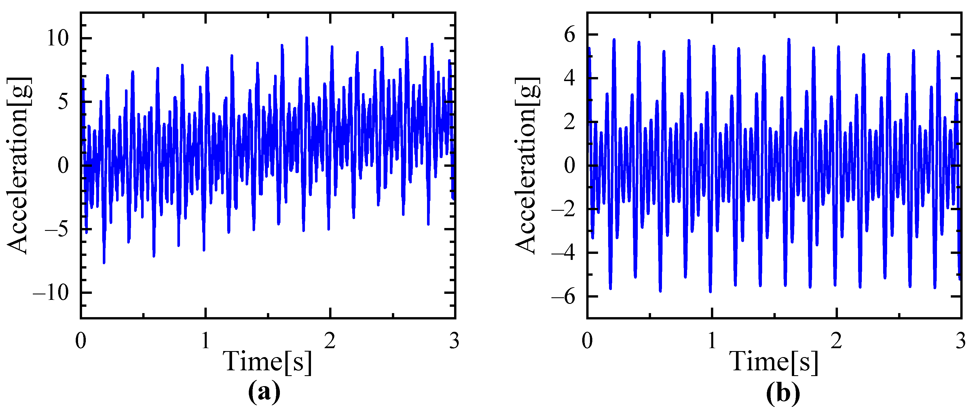
2.2. Elimination of Trend Items and De-Noising
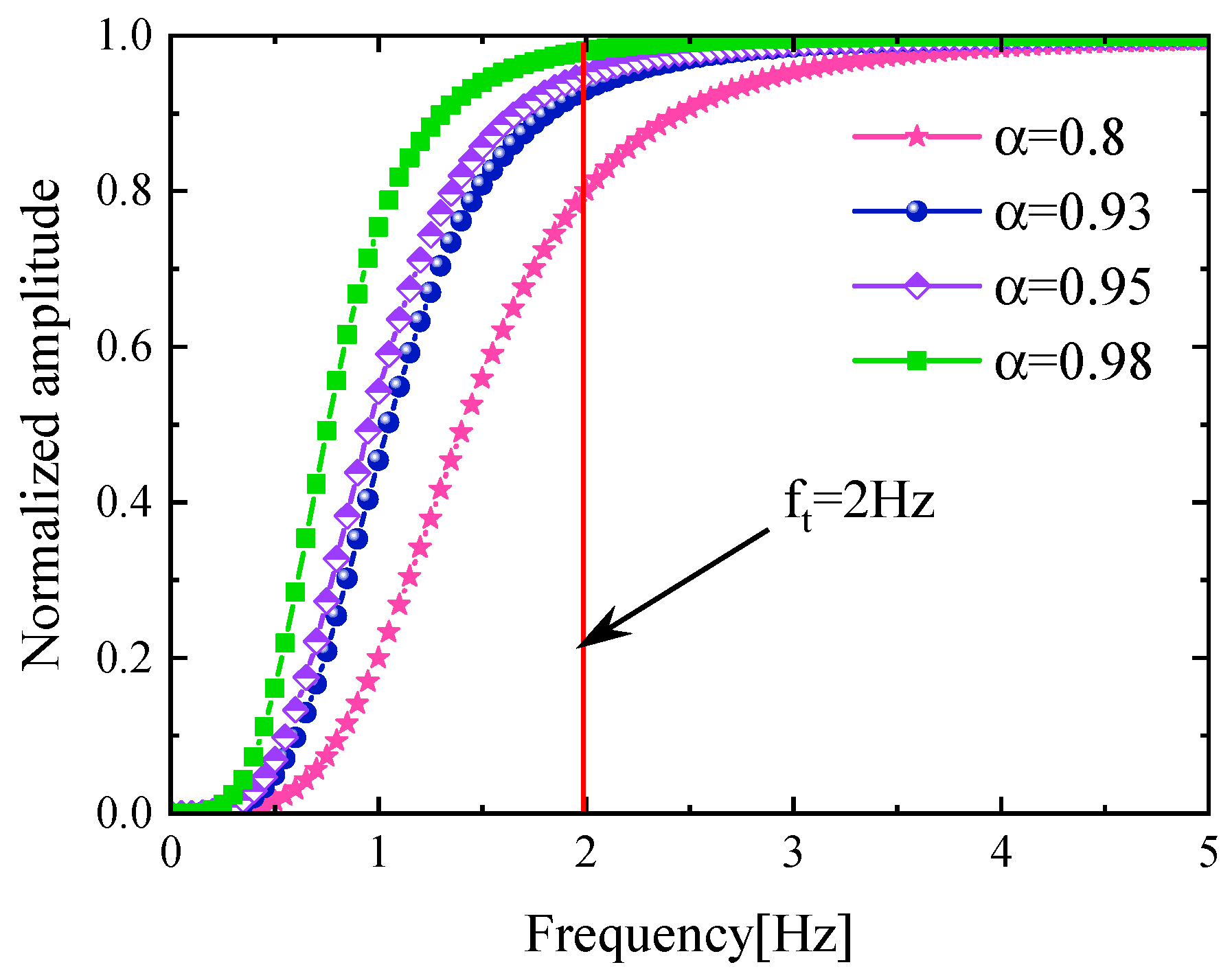
2.3. Digital Filtering and Frequency Domain Integration
3. Modal Parameter Identification
3.1. State Space Model of Structural Vibration
3.2. Identification of the Hankel Matrix
3.3. Extraction and Selection of Modes
3.4. Improved Stochastic Subspace Identification Algorithm
- (1)
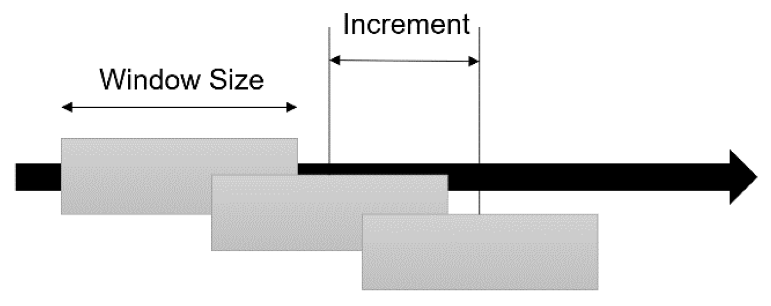
- Assume that the initial window time is , the sampling frequency is sf, and the initial window length is .
- (2)
- Let the lag time, , between previous and later windows and the data length correspond to the ith window, as .
- (3)
- Identify the corresponding stability diagrams of each window by the SSI algorithm. If the system order is N, the maximum number of stable points will be the same corresponding to each mode. The related number of stable points for the first three modes are , , and , and the percentages, , of these modes can be obtained.
- (4)
- Change the value of with the signal length. When the percentage exceeds 90%, the corresponding window time is supposed to be the appropriate one, otherwise the window time will be increased.
4. Numerical Simulation
4.1. Synthesized Ideal Discrete Acceleration
4.2. 3-DOF Mass-Damping-Spring System
5. Experimental Verification
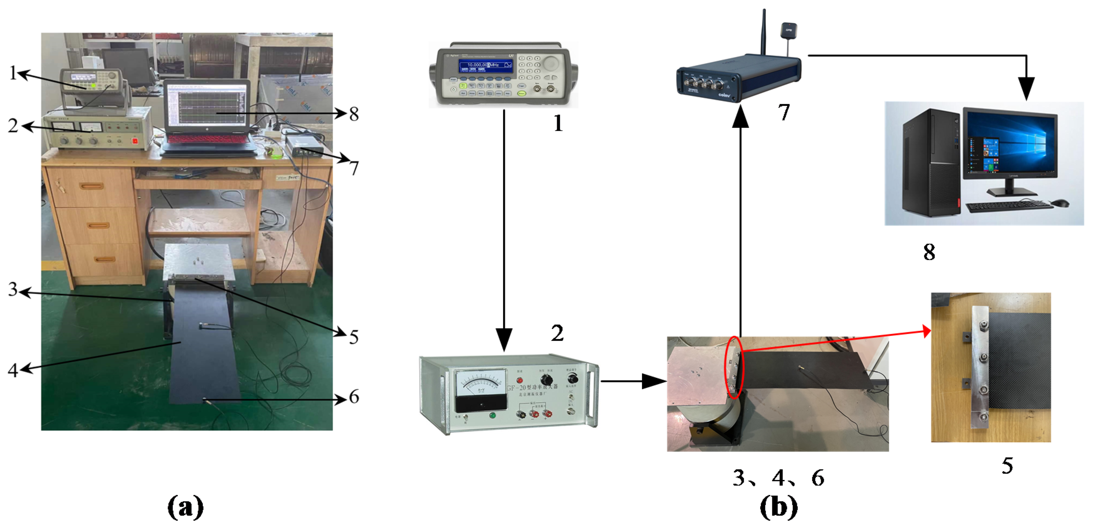
5.1. Experimental Setup
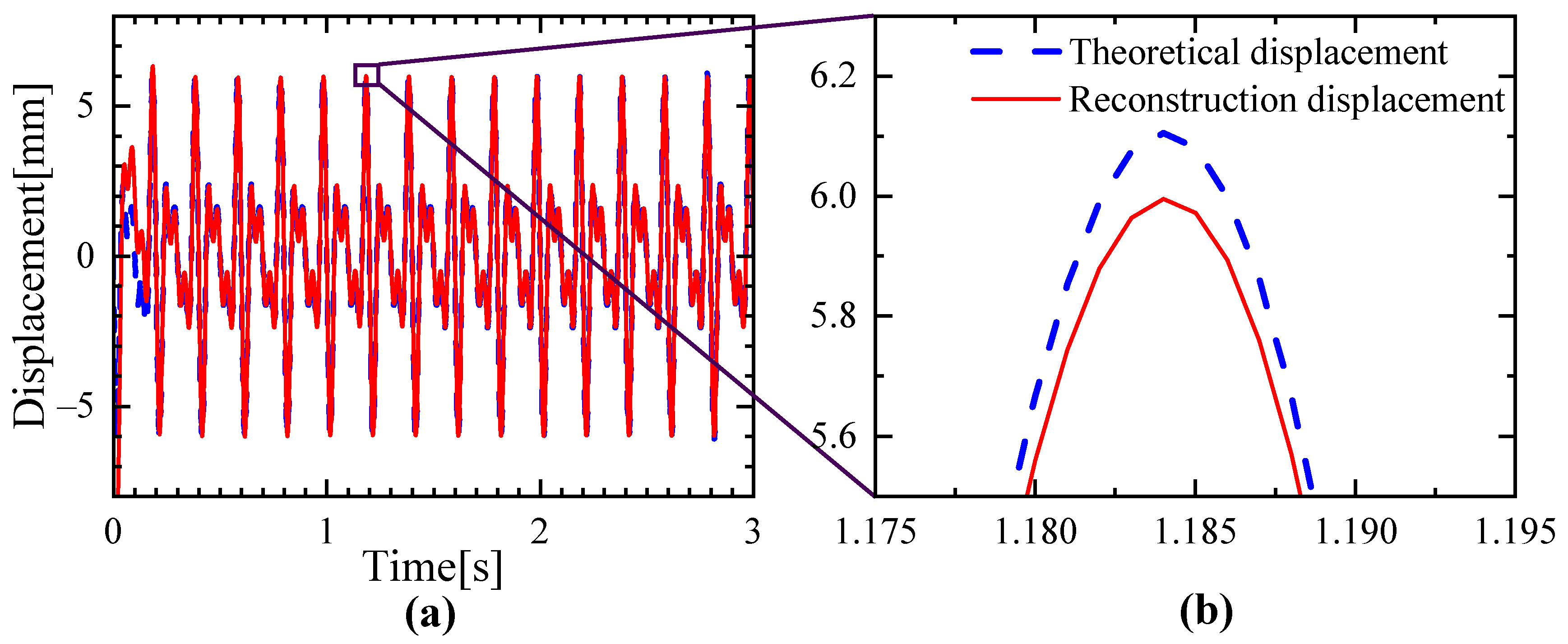
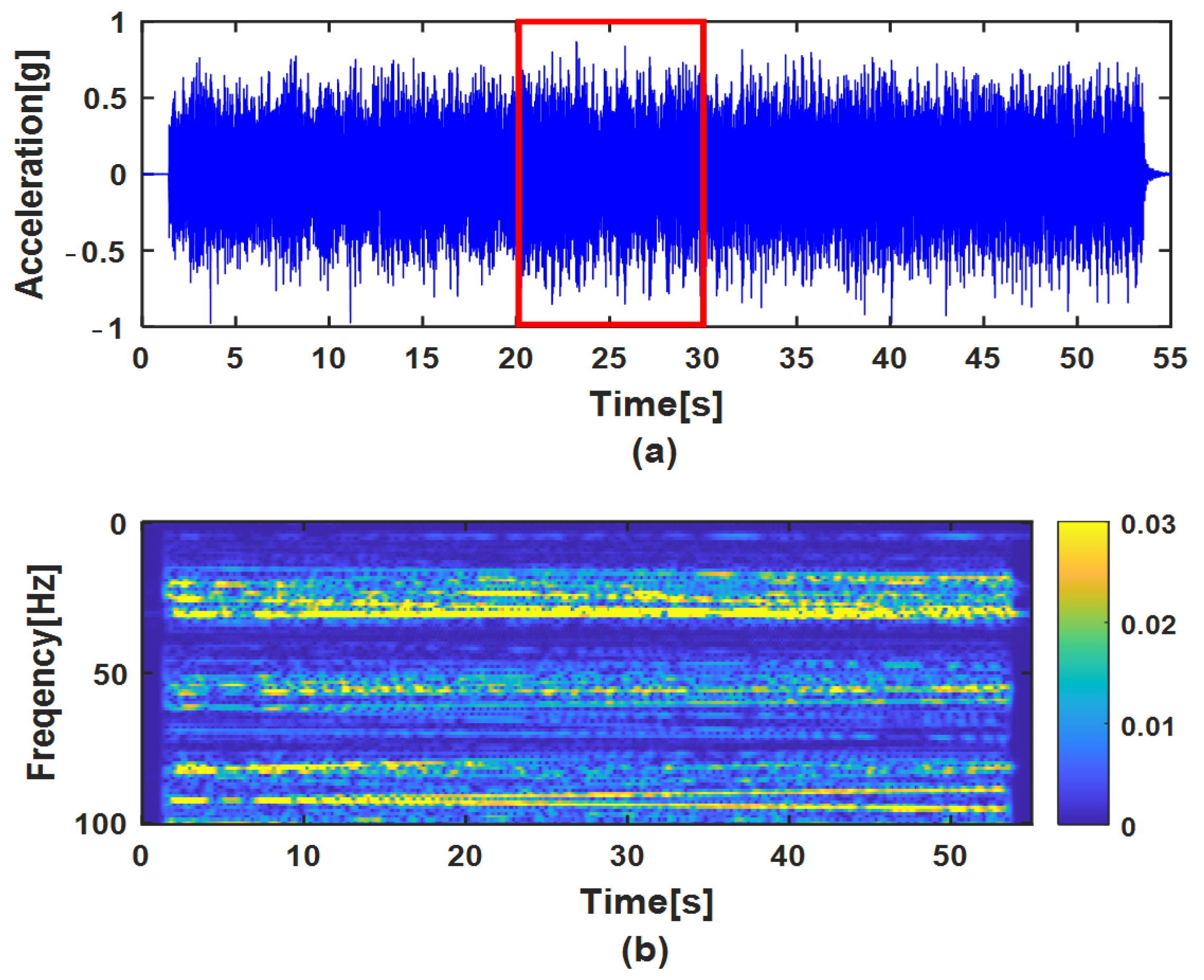
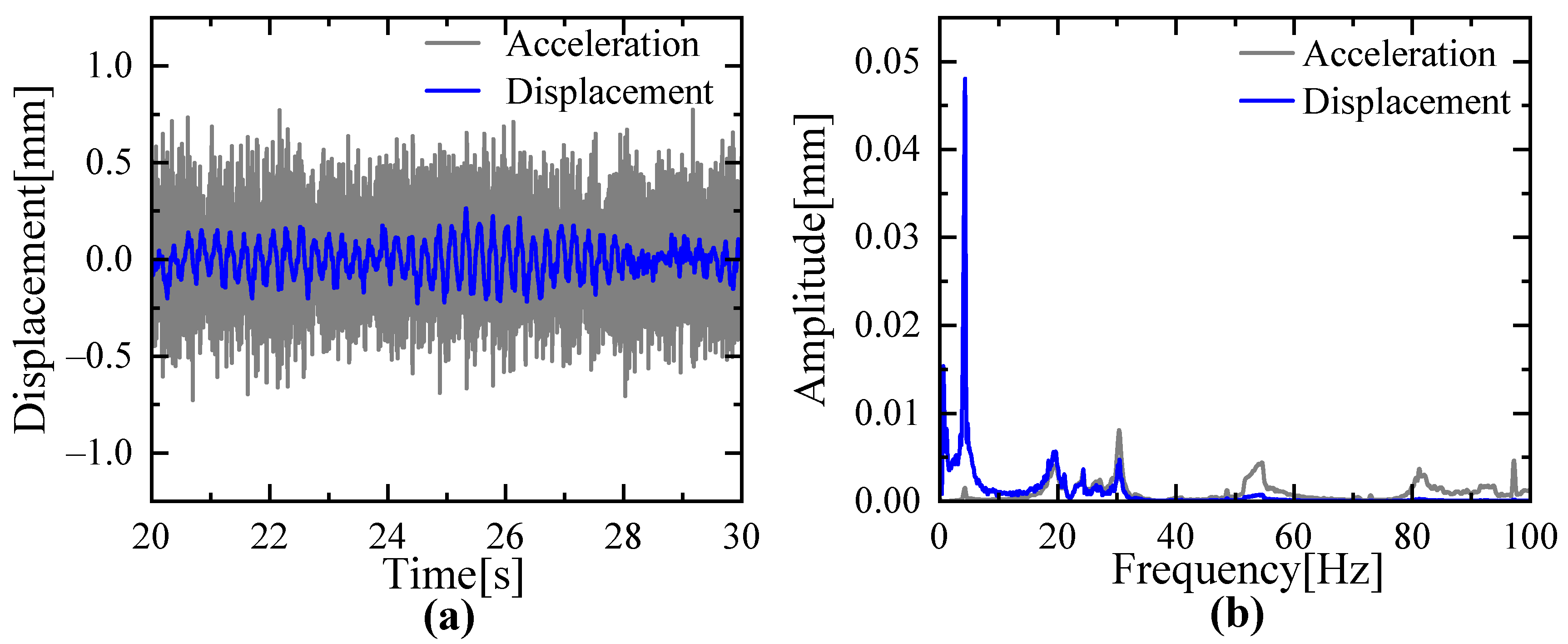
5.2. Reconstructed Displacements Calculated from Accelerations
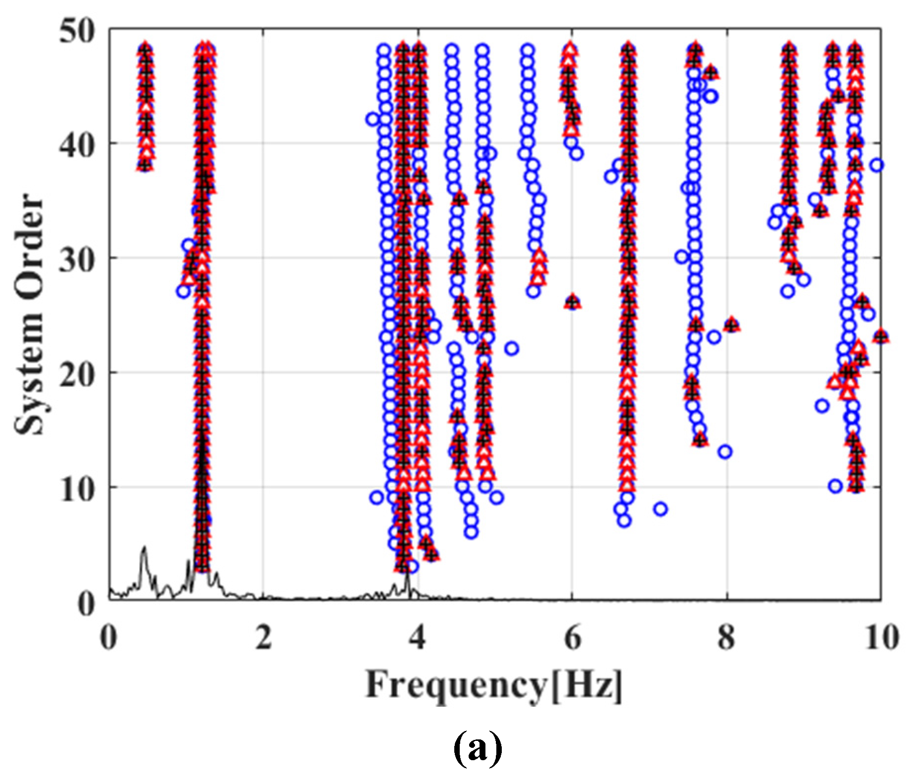
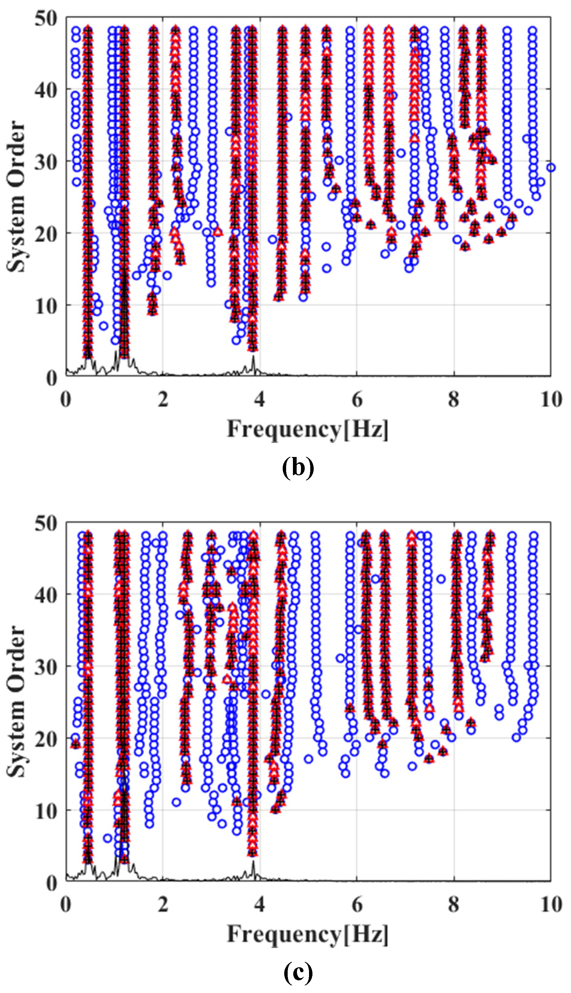
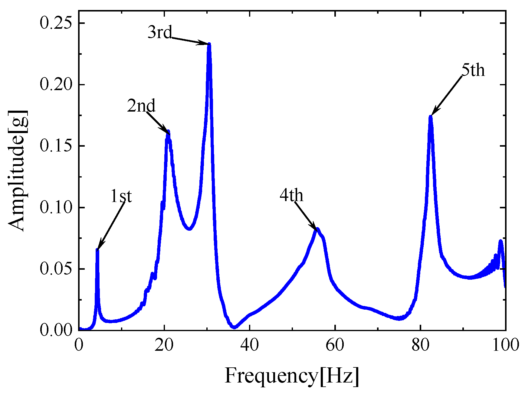
5.3. Modal Parameter Identification
6. Conclusions
- In comparison to the acceleration-based modal parameter identification method, the proposed method based on reconstructed displacements could suppress high-frequency components and reduce the non-stationary characteristics of measured data more effectively. Therefore, this method could provide more reliable and accurate parameter identification results for small model order selection.
- In comparison to other integration methods, the proposed method had no error accumulation and long period drift of reconstructed displacements, resulting in higher computational efficiency.
- Experimental results of the cantilever plate revealed that the improved SSI method could improve the recognition efficiency and also identify more stable results for low-frequency structures.
Author Contributions
Funding
Institutional Review Board Statement
Informed Consent Statement
Data Availability Statement
Acknowledgments
Conflicts of Interest
References
- He, Y.C.; Li, Z.; Fu, J.Y.; Wu, J.R.; Ng, C.T. Enhancing the performance of stochastic subspace identification method via energy-oriented categorization of modal components. Eng. Struct. 2021, 233, 111917. [Google Scholar] [CrossRef]
- Storti, G.C.; Carrer, L.; Silva Tuckmantel, F.W.; Machado, T.H.; Cavalca, K.L.; Bachschmid, N. Simulating application of operational modal analysis to a test rig. Mech. Syst. Signal Process. 2021, 153, 107529. [Google Scholar] [CrossRef]
- Liu, F.S.; Gao, S.J.; Han, H.W.; Tian, Z.; Liu, P. Interference reduction of high-energy noise for modal parameter identification of offshore wind turbines based on iterative signal extraction. Ocean Eng. 2019, 183, 372–383. [Google Scholar] [CrossRef]
- Aulakh, D.S.; Bhalla, S. 3D torsional experimental strain modal analysis for structural health monitoring using piezoelectric sensors. Measurement 2021, 180, 109476. [Google Scholar] [CrossRef]
- Uehara, D.; Sirohi, J. Full-field optical deformation measurement and operational modal analysis of a flexible rotor blade. Mech. Syst. Signal Process. 2019, 133, 106265. [Google Scholar] [CrossRef]
- Orlowitz, E.; Brandt, A. Comparison of experimental and operational modal analysis on a laboratory test plate. Measurement 2017, 102, 121–130. [Google Scholar] [CrossRef]
- Boonyapinyo, V.; Janesupasaeree, T. Data-driven stochastic subspace identification of flutter derivatives of bridge decks. J. Wind Eng. Ind. Aerodyn. 2010, 98, 784–799. [Google Scholar] [CrossRef]
- Ni, Z.Y.; Liu, J.G.; Wu, S.N.; Wu, Z.G. Time-varying state-space model identification of an on-orbit rigid-flexible coupling spacecraft using an improved predictor-based recursive subspace algorithm. Acta Astronaut. 2019, 163, 157–167. [Google Scholar] [CrossRef]
- Jin, N.; Yang, Y.B.; Dimitrakopoulos, E.G.; Paraskeva, T.S.; Katafygiotis, L.S. Application of short-time stochastic subspace identification to estimate bridge frequencies from a traversing vehicle. Eng. Struct. 2021, 230, 111688. [Google Scholar] [CrossRef]
- Li, J.T.; Zhu, X.Q.; Law, S.; Samali, B. Indirect bridge modal parameters identification with one stationary and one moving sensors and stochastic subspace identification. J. Sound Vib. 2019, 446, 1–21. [Google Scholar] [CrossRef]
- Yan, R.Q.; Gao, R.X.; Zhang, L. In-process modal parameter identification for spindle health monitoring. Mechatronics 2015, 31, 42–49. [Google Scholar] [CrossRef] [Green Version]
- Fang, Z.; Su, H.Z.; Ansari, F. Modal analysis of structures based on distributed measurement of dynamic strains with optical fibers. Mech. Syst. Signal Process. 2021, 159, 107835. [Google Scholar] [CrossRef]
- Priori, C.; Angelis, M.D.; Betti, R. On the selection of user-defined parameters in data-driven stochastic subspace identification. Mech. Syst. Signal Process. 2018, 100, 501–523. [Google Scholar] [CrossRef]
- Wen, P.; Khan, I.; He, J.; Chen, Q.F. Application of Improved Combined Deterministic-Stochastic Subspace Algorithm in Bridge Modal Parameter Identification. Shock Vib. 2021, 11, 8855162. [Google Scholar] [CrossRef]
- Zhou, Y.L.; Jiang, X.L.; Zhang, M.J.; Zhang, J.X.; Sun, H.; Li, X. Modal parameters identification of bridge by improved stochastic subspace identification method with Grubbs criterion. Meas. Control 2021, 54, 457–464. [Google Scholar] [CrossRef]
- Gres, S.; Döhler, M.; Andersen, P.; Mevel, L. Kalman filter-based subspace identification for operational modal analysis under unmeasured periodic excitation. Mech. Syst. Signal Process. 2021, 146, 106996. [Google Scholar] [CrossRef]
- Tran, T.T.X.; Ozer, E. Synergistic bridge modal analysis using frequency domain decomposition, observer Kalman filter identification, stochastic subspace identification, system realization using information matrix, and autoregressive exogenous model. Mech. Syst. Signal Process. 2021, 160, 107818. [Google Scholar] [CrossRef]
- Kim, S.; Park, K.Y.; Kim, H.K.; Lee, H.S. Damping estimates from reconstructed displacement for low-frequency dominant structures. Mech. Syst. Signal Process. 2020, 136, 106533. [Google Scholar] [CrossRef]
- Gao, S.J.; Liu, F.S.; Jiang, C.Y. Improvement study of modal analysis for offshore structures based on reconstructed displacements. Appl. Ocean Res. 2021, 110, 102596. [Google Scholar] [CrossRef]
- Liu, F.S.; Li, H.J.; Li, W.; Yang, D.P. Lower-order modal parameters identification for offshore jacket platform using reconstructed responses to a sea test. Appl. Ocean Res. 2014, 46, 124–130. [Google Scholar] [CrossRef]
- Zhu, H.; Zhou, Y.J.; Hu, Y.M. Displacement reconstruction from measured accelerations and accuracy control of integration based on a low-frequency attenuation algorithm. Dyn. Earthq. Eng. 2020, 133, 106122. [Google Scholar] [CrossRef]
- Lee, H.S.; Hong, Y.H.; Park, H.W. Design of an FIR filter for the displacement reconstruction using measured acceleration in low-frequency dominant structures. Int. J. Numer. Methods Eng. 2010, 82, 403–434. [Google Scholar] [CrossRef]
- Hong, Y.H.; Lee, S.G.; Lee, H.S. Design of the FEM-FIR filter for displacement reconstruction using accelerations and displacements measured at different sampling rates. Mech. Syst. Signal Process. 2013, 38, 460–481. [Google Scholar] [CrossRef]
- Park, K.Y.; Lee, H.S. Design of de-noising FEM-FIR filters for the evaluation of temporal and spatial derivatives of measured displacement in elastic solids. Mech. Syst. Signal Process. 2019, 120, 524–539. [Google Scholar] [CrossRef]
- Brandt, A.; Brincker, R. Integrating time signals in frequency domain comparison with time domain integration. Measurement 2014, 58, 511–519. [Google Scholar] [CrossRef]
- Thong, Y.K.; Woolfson, M.S.; Crowe, J.A.; Hayes-Gill, B.R.; Jones, D.A. Numerical double integration of acceleration measurements in noise. Measurement 2004, 36, 73–92. [Google Scholar] [CrossRef]
- Reynders, E.P.B. Uncertainty quantification in data-driven stochastic subspace identification. Mech. Syst. Signal Process. 2021, 151, 107338. [Google Scholar] [CrossRef]
- Xu, Y.F.; Zhu, W.D. Operational modal analysis of a rectangular plate using non-contact excitation and measurement. J. Sound Vib. 2013, 332, 4927–4939. [Google Scholar] [CrossRef]
- Zheng, W.H.; Dan, D.H.; Cheng, W.; Xia, Y. Real-time dynamic displacement monitoring with double integration of acceleration based on recursive least squares method. Measurement 2019, 141, 460–471. [Google Scholar] [CrossRef]
- Hu, Z.X.; Li, J.; Zhi, L.H.; Huang, X. Modal Identification of damped vibrating systems by iterative smooth orthogonal decomposition method. Adv. Struct. Eng. 2021, 24, 755–770. [Google Scholar] [CrossRef]


| Maximum Error | Frequency | |||||
|---|---|---|---|---|---|---|
| 0.2 Hz | 0.5 Hz | 1 Hz | 4 Hz | 8 Hz | ||
| Precision Coefficient | 0.92 | 0.059 | 0.025 | 0.013 | 0.016 | 0.015 |
| 0.95 | 0.054 | 0.023 | 0.012 | 0.015 | 0.016 | |
| 0.98 | 0.047 | 0.021 | 0.011 | 0.017 | 0.020 | |
| Carbon Fiber Composite | |||
|---|---|---|---|
| Young’s modulus (GPa) | Ex | Ey | Ez |
| 47.45 | 60.3 | 3.9 | |
| Shear modulus (GPa) | Gxy | Gyz | Gxz |
| 72.9 | 1.5 | 62.35 | |
| Poisson’s ratio | νxy | νyz | νxz |
| 0.3 | 0.4 | 0.3 | |
| Density (Kg/m3) | 1800 | ||
| Calculated by Sinusoidal Sweeps | Calculated by Accelerations | Calculated by Displacements | By the Method of He [1] | ||
|---|---|---|---|---|---|
| First-order | Frequency (Hz) | 4.304 | 4.013 | 4.407 | 4.535 |
| Damping ratio | 2.10% | 1.42% | 2.31% | 2.90% | |
| Second-order | Frequency (Hz) | 20.839 | 20.241 | 20.189 | 20.351 |
| Damping ratio | 3.68% | 2.71% | 3.49% | 4.20% | |
| Third-order | Frequency (Hz) | 30.518 | 30.256 | 30.188 | 30.258 |
| Damping ratio | 2.30% | 1.55% | 1.50% | 3.50% | |
| Fourth-order | Frequency (Hz) | 55.839 | 51.821 | 55.449 | 53.556 |
| Damping ratio | 3.88% | 4.80% | 3.50% | 5.10% |
Publisher’s Note: MDPI stays neutral with regard to jurisdictional claims in published maps and institutional affiliations. |
© 2021 by the authors. Licensee MDPI, Basel, Switzerland. This article is an open access article distributed under the terms and conditions of the Creative Commons Attribution (CC BY) license (https://creativecommons.org/licenses/by/4.0/).
Share and Cite
Guo, X.; Li, C.; Luo, Z.; Cao, D. Modal Parameter Identification of Structures Using Reconstructed Displacements and Stochastic Subspace Identification. Appl. Sci. 2021, 11, 11432. https://doi.org/10.3390/app112311432
Guo X, Li C, Luo Z, Cao D. Modal Parameter Identification of Structures Using Reconstructed Displacements and Stochastic Subspace Identification. Applied Sciences. 2021; 11(23):11432. https://doi.org/10.3390/app112311432
Chicago/Turabian StyleGuo, Xiangying, Changkun Li, Zhong Luo, and Dongxing Cao. 2021. "Modal Parameter Identification of Structures Using Reconstructed Displacements and Stochastic Subspace Identification" Applied Sciences 11, no. 23: 11432. https://doi.org/10.3390/app112311432
APA StyleGuo, X., Li, C., Luo, Z., & Cao, D. (2021). Modal Parameter Identification of Structures Using Reconstructed Displacements and Stochastic Subspace Identification. Applied Sciences, 11(23), 11432. https://doi.org/10.3390/app112311432