Bead Geometry Prediction in Laser-Wire Additive Manufacturing Process Using Machine Learning: Case of Study

Featured Application

Laser Wire Additive Manufacturing.

Abstract

In Laser Wire Additive Manufacturing (LWAM), the final geometry is produced using the layer-by-layer deposition (beads principle). To achieve good geometrical accuracy in the final product, proper implementation of the bead geometry is essential. For this reason, the paper focuses on this process and proposes a layer geometry (width and height) prediction model to improve deposition accuracy. More specifically, a machine learning regression algorithm is applied on several experimental data to predict the bead geometry across layers. Furthermore, a neural network-based approach was used to study the influence of different deposition parameters, namely laser power, wire-feed rate and travel speed on bead geometry. To validate the effectiveness of the proposed approach, a test split validation strategy was applied to train and validate the machine learning models. The results show a particular evolutionary trend and confirm that the process parameters have a direct influence on the bead geometry, and so, too, on the final part. Several deposition parameters have been found to obtain an accurate prediction model with low errors and good layer deposition. Finally, this study indicates that the machine learning approach can efficiently be used to predict the bead geometry and could help later in designing a proper controller in the LWAM process.

1. Introduction

Additive manufacturing (AM) is the process of depositing materials layer-by-layer to produce a part, as against subtractive manufacturing, which starts from a block of raw material, removing small parts to obtain the final product. The drawbacks of the subtractive method are its material waste and geometric limitations in creating complex geometries [1]. Laser Wire Additive Manufacturing (LWAM), also referred to as Laser Wire-Feed Metal Additive Manufacturing (LWMAM), is a variant of the Direct Energy Deposition (DED) method. DED creates parts by melting the material into a molten metal pool [2]. LWAM uses a wire-metal feed-stock and a laser source to create the molten pool, as shown in Figure 1. It usually requires a shroud of shielding gas to protect the deposition from contamination. Metal wires offer an environmentally friendly process by being cleaner, more cost-competitive, cheaper, and more abundant than metal powders. In addition to being identical to the wire used in welding applications, a standardized and qualified product can be obtained. Additionally, the wire-feed approach, in comparison with the arc-welding approachm affords a larger build volume at high productivity [3,4].

There is a growing interest in the aeronautical sector to find methods to create complex large parts that lead to the improvement of the buy-to-fly ratio [5]. Therefore, it becomes essential to improve process planning and deposition strategies to get an optimal combination of parameters involved in the LWAM process. One of them is layer geometry. When it is well defined, layer height and width improve the part’s geometric accuracy and the surface quality of the product [6]. Figure 2 illustrates the flow path of process planning for LWAM. The importance of the prediction model for the whole LWAM process should be noted; this model can influence, for example, the method by which process parameters are chosen and optimized, improving the surface quality of the final product. Furthermore, the tool’s path can be adjusted based on the obtained model and can be utilized when generating the robot code. Thus, if a predictive model can be implemented properly, it will lead to products of higher quality and productivity increases [7].

Methodologies for solving the issue of predicting layer geometry during the deposition process are divided into two approaches. The first approach uses numerical or mathematical models, wherein the layer deposition is predicted from experimental processes. The second approach uses sensing devices to develop control algorithms that regulate process parameters, such as laser power, the wire feed rate, travel speed and others during the printing process. The feedback control approach is commonly used in industry and employs sensors such as pyrometers or camera vision systems to monitor the melt-pool characteristics and temperature of the deposition [8,9,10]. Much research [11,12,13,14,15,16] has been reported on the use of the control approach to monitor the deposition parameters to minimize observed fluctuation and keep a controlled deposition environment. However, such an approach is not always feasible, due to process uncertainties and variations occurring during the deposition process that augment the system’s complexity. Also, sensing devices face some delay in acquiring information from the system and further delay is observed when transferring data between devices and analyzing the information before the control action. Another constraint occurs in the melt pool when laser reflection and conducted heat add complexity to the information acquisition [17]. A literature survey has confirmed this, (e.g., [6,7]) since the majority of validation using this approach is performed for simply shaped structures, focusing on only one parameter.

On the other hand, the mathematical and numerical approach relies on the use of generic equations or simulations to study different deposition scenarios and see the influence of the layer geometry on the final produced part [18,19,20,21,22,23]. To improve the surface quality of the deposition Zhu et al. [24] investigated the influence of varying the laser’s power and defocusing distance on deposition. The laser power was decreased at each layer to avoid energy accumulation and reduce the pool size change. Additionally, the same layer thickness was used. This approach yields differences in the top layer when changing defocusing distances due to fluctuating parameters and system error. This is due to the height difference observed between layers, which propagate to the other layers, becoming increasingly pronounced if the difference is not compensated for, hence, the necessity of self-regulating deposition height. As layer thickness needs to be adjusted to satisfy the process’s growth, Donadello et al. [25] proposed a reconstruction of the spatial map of the height to see the variation of the layer thickness and found a self-regulating mechanism therein; after an initial transient period showing faster deposition growth in the first layers, deposition rate exhibits a decreasing trend until converging to steady-state, interpreted as an equilibrium condition, is achieved. In this approach, although there exist disturbances from system sensitivity and error, the self-regulating mechanism occurring during the deposition process is obvious. For this reason, the problem of height prediction should be solved in advance of regulating those process parameters occupying a primary level in the 3D printing process.

Machine learning (ML) is applied in many domains, today. Many industrial sectors face new research challenges and complex problems yet to be addressed. The advantage of ML is demonstrated in areas where underlying physical models are difficult to express. The neural network (NN) algorithm is the most used ML method due to its advanced algorithm structure [26]. NNs can be used as supervised ML or unsupervised learning problems for complex problems with highly nonlinear relationships. The architecture of an NN consists of the input layer, a hidden layer, and an output layer [27]. The layers are composed of nodes or neurons. In Khatir et al. [28], an improved artificial neural network (ANN) using arithmetic optimization algorithm (IANN-AOA) for damage quantification problems is proposed. Free vibration and damage identification have been investigated on functionally graded material (FGM) plates, while, in [29], damaged laminated composite structures are identified using an ANN. In this approach, the network is trained using fast convergence speed of gradient descent (GD) techniques and the global search capacity of evolutionary algorithms EAs is used to quickly guarantee the best possible solution. Finally, Zenzen et al. [30] implemented a modified transmissibility damage indicator using local frequency response ratio (LFCR) and ANN to detect the location and size of damage in composite structures while reducing collected data for fast prediction and high accuracy.

Recently, researchers have worked on the bead geometry prediction models using machine learning approaches to address issues relating to deposition accuracy [7,31,32,33,34,35]. Xiong et al. [31] used second-order regression with a neural network for predicting bead geometry in wire and arc additive manufacturing (WAAM) to study the relationship between the process variables and the final bead geometry. While Nagesh and Datta [32] used the back propagation (BP) neural network model for estimating bead geometry for tungsten inert gas (TIG) welding process. Xia et al. [7] developed a roughness measuring method for arc additive manufacturing using a laser sensor-based approach combined with different machine learning models. On the other hand, Milhomme et al. [33] studied first-order parameters to identify correlations between input parameters and geometrical outputs of Ti-6Al-4V beads manufactured with the laser metal powder deposition process. Finally, Karmuhilan and Kumarsood [34] discussed the use of an artificial neural network (ANN) to predict the bead parameters based on given process parameters for the WAAM system.

From the above literature review, one can conclude that the machine learning approach and, more particularly, NNs, have not been applied to LWAM bead geometry prediction considering deposition parameters that influence both the bead width and the height of the produced part. This is due to the complexity of layer deposition stability and the high feed rate of the LWAM process in comparison with other techniques, such as WAAM [36]. Therefore, this paper aims to provide a machine learning approach using a regression algorithm to predict the layer geometry in the LWAM process. Different experiments are performed to deposit sample products and, with the developed prediction model, the height, width, and ratios for upcoming layers are proposed. Furthermore, the influence of the deposition parameters (laser power, wire feed rate and travel speed) on the final produced geometry is discussed based on a neural network prediction model. This case study could provide inspiration and guidance for improving surface roughness in LWAM using a proper feedback control system.

For proper implementation of the prediction algorithm, we employ a technique used by Lim et al. [37] for collecting the data. The method uses scripting languages to propose a method of slicing layers and generating printing paths. The use of the parametric method is adopted to generate printing paths using Rhino’s Grasshopper environment (see Figure 2). In Lim et al.’s approach, the prospect of flexibility in model design provides more opportunities for the designer to decide on the size and shape of the layer (flat or curved), path patterns, and other parameters affecting the surface’s geometrical quality and printing time. However, this proposal could be improved by taking into consideration the height variation mentioned in Lim et al.’s work and, especially, by finding a way to avoid many of the issues found with G-Code (see e.g., [38]), as well as communicating directly to the printing machine in terms of AM using an industrial robot.

The paper is structured as follows, Section 2 introduces the global approach of the methodology, while Section 3 provides a detailed theoretical background for the proposed prediction model. Section 4 presents the experimental results and discussion. The paper finishes in Section 5 by a conclusion and a proposal of future work.

2. Methodology

In this paper, the bead geometry measurements for different layers have been obtained using Grasshopper software. Grasshopper uses generative algorithms and parametric modeling that differentiates it from other CAD software, which uses polygon mesh-based representations to model an object. More specifically, Rhino’s Grasshopper was used to create the physical part specifications (bead size, layer height, pattern, etc.). Then generative algorithm was implemented and converted to robot programs using the HAL framework. This approach was chosen because the programming methodology interface is suitable for mathematical representations without passing through the G-Code step [39]. This is done using the following steps:

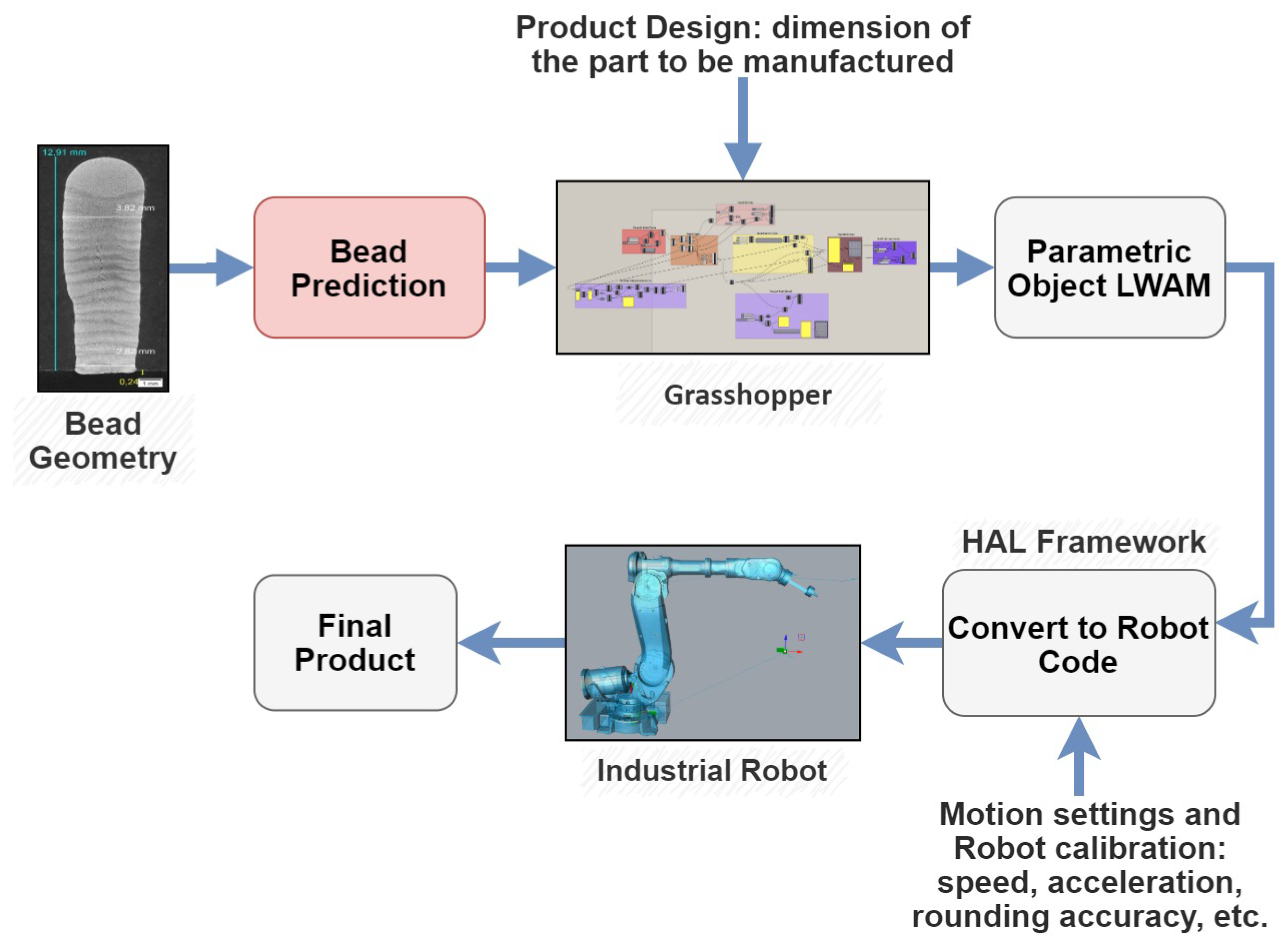
• Parametric surface creation: In this step, mathematical tools are used to create a 2D model surface. Alternatively, a CAD part could be imported directly and changed to a parametric CAD part using Grasshoppers tools.
• Pattern creation: In this step, patterns (zigzag, spiral tool path, etc.) are designed and added to the 2D surface. The zigzag pattern is advised for its simplicity of implementation, robustness, and surface roughness [40].
• Layer-to-layer deposition strategy: After depositing the first layer, a suitable travel strategy is required to reach the next layer, and successively. The travel strategy depends on some deposition parameters, such as the laser power, wire feed rate, and robot travel speed. Therefore, the travel strategy should be carefully chosen as it can influence the cooling of the previous layer as well as the bonding between layers. For more details see e.g., [41,42].
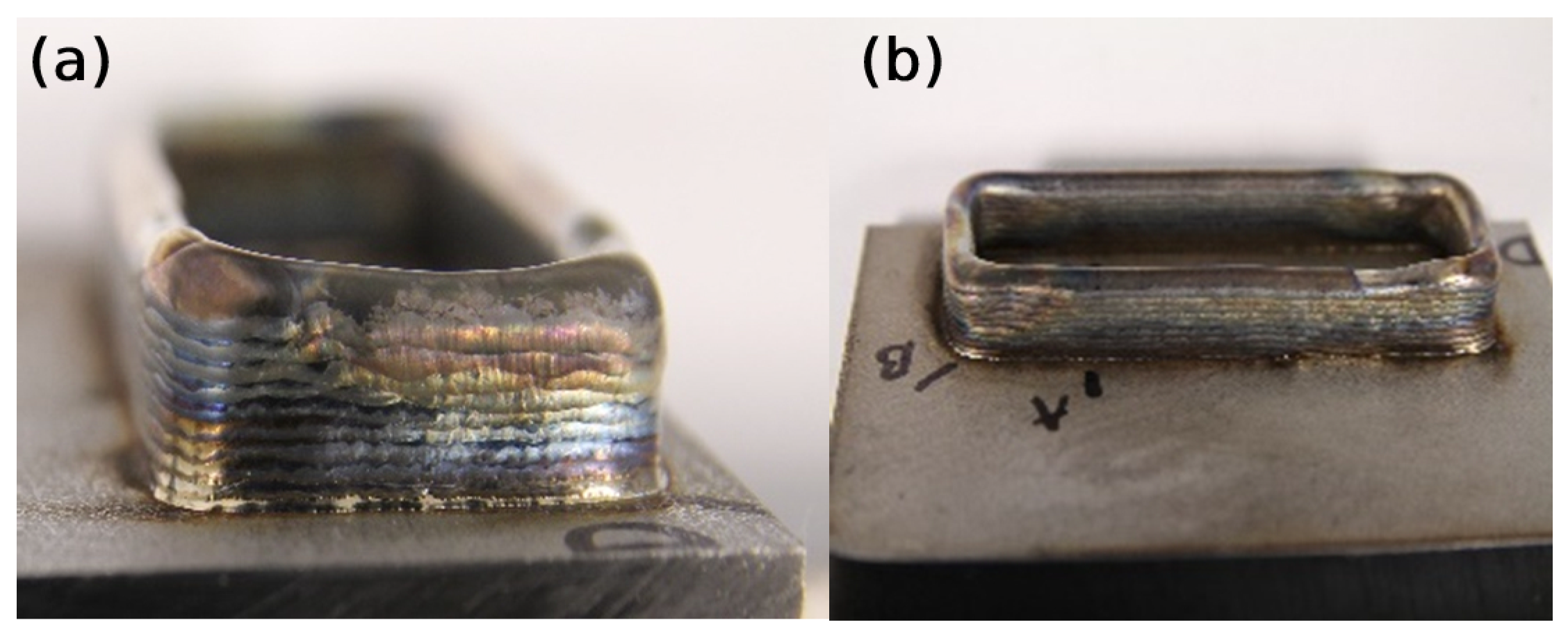
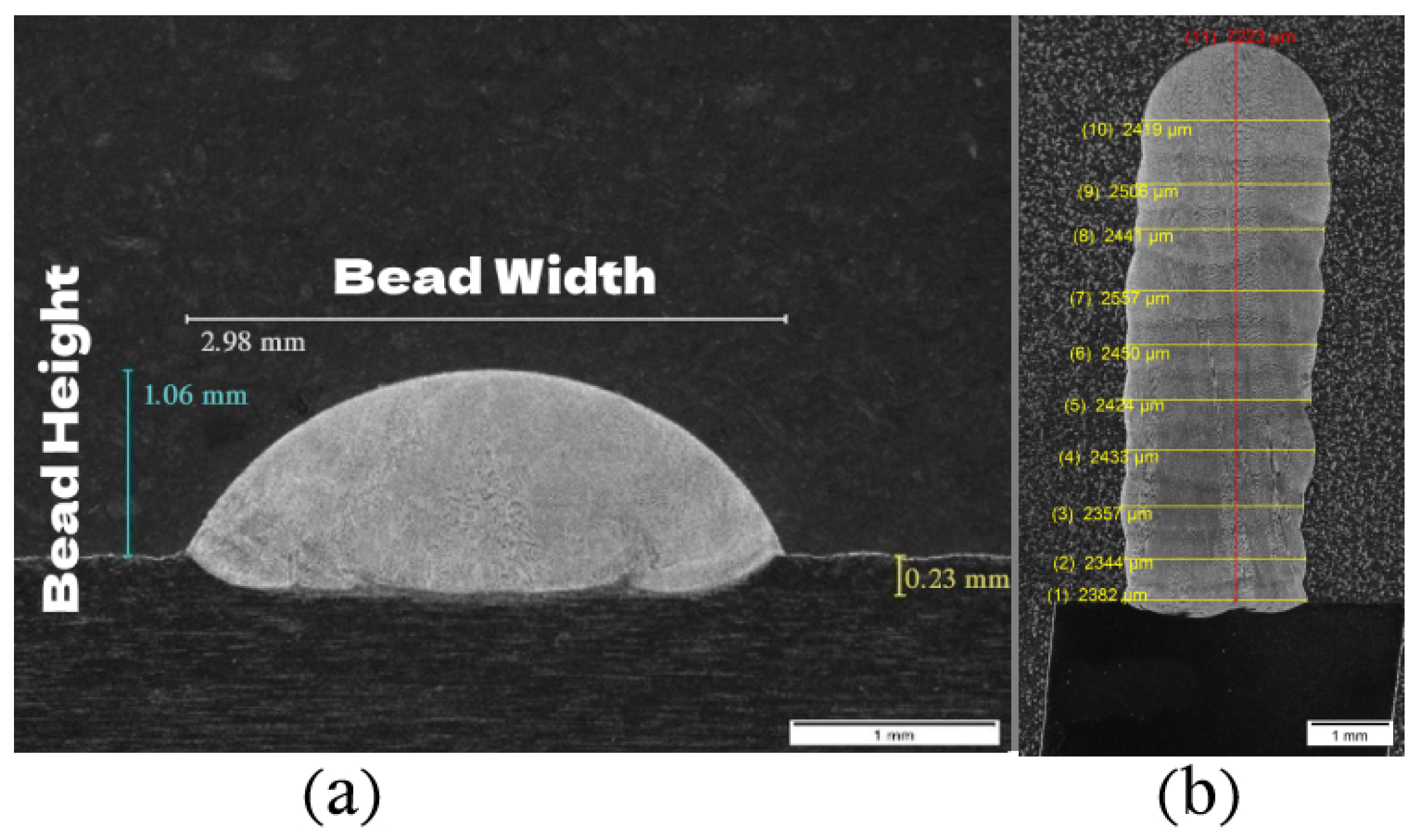
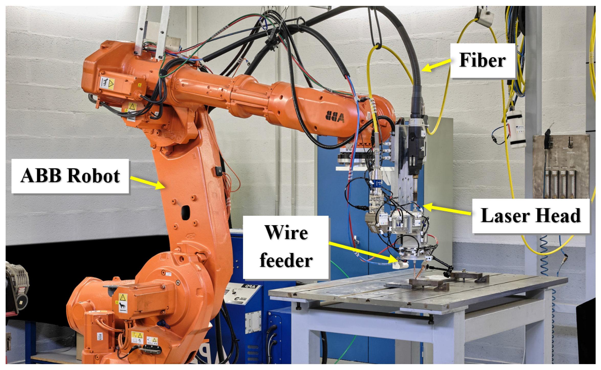
• Bead geometry measurements: Finally, a laser scanner was used to obtain the measurements data of the bead geometry during the LWAM process. The laser scanner was mounted on the welding robot’s arm to directly measure the bead geometry for each layer deposition. A measurement for a single bead geometry and layer deposition is shown in Figure 3.

After having several bead’s geometry measurements and dimensions, a prediction function $F\left(x\right)$, based on a regression algorithm, is used to predict the bead geometry for the current layer and the successive layers. The prediction function $F\left(x\right)$ can then be fed to Grasshopper with two more inputs, the product design specification and the bead dimensions. Next, the designed parametric object is loaded to the HAL framework and converted to a robot program, along with the motion settings and the robot calibration. Finally, a simulated 3D printing program of the final product is ready to be transferred to the real robot to begin manufacturing 3D parts, as shown in Figure 2.

The prediction algorithm, used in this work, includes linear regression and linearization steps for non-linear trend (power decay function). The power decaying function is used to represent the self-regulation of the layer geometry. The prediction model takes as input the training examples ($x_i$, $i=1$ to m, $m=$ final layer geometry dimension) and the output is the model prediction that relates the bead geometry changes over layer depositions.

Finally, a neural network technique was used to correlate the bead geometry measurements with the first-order deposition parameters: laser power, wire feed rate, and travel speed. In this way, the prediction algorithm method (discussed in Section 3.1) was used first with the fixed deposition parameters, and then a neural network (discussed in Section 3.2) was used with varied deposition parameters to study their influence on bead geometry.

3. Prediction Model

To predict the bead geometry for a given sample, a supervised-learning algorithm is employed. Supervised learning is efficient for problems for which it is possible to find a closed-form solution between the inputs and outputs. The geometry prediction is taken as a regression problem in which a mathematical function is derived from a training set.

In this work, a power decay function is used to represent the prediction function and solve the self-regulation mechanism occurring in the deposition process. Furthermore, bead height, width and width-height ratio prediction models are obtained for different deposition parameters. However, since the same algorithm and technique is used for all prediction models, in this section height prediction equations will be discussed and other prediction models equations are omitted for brevity.

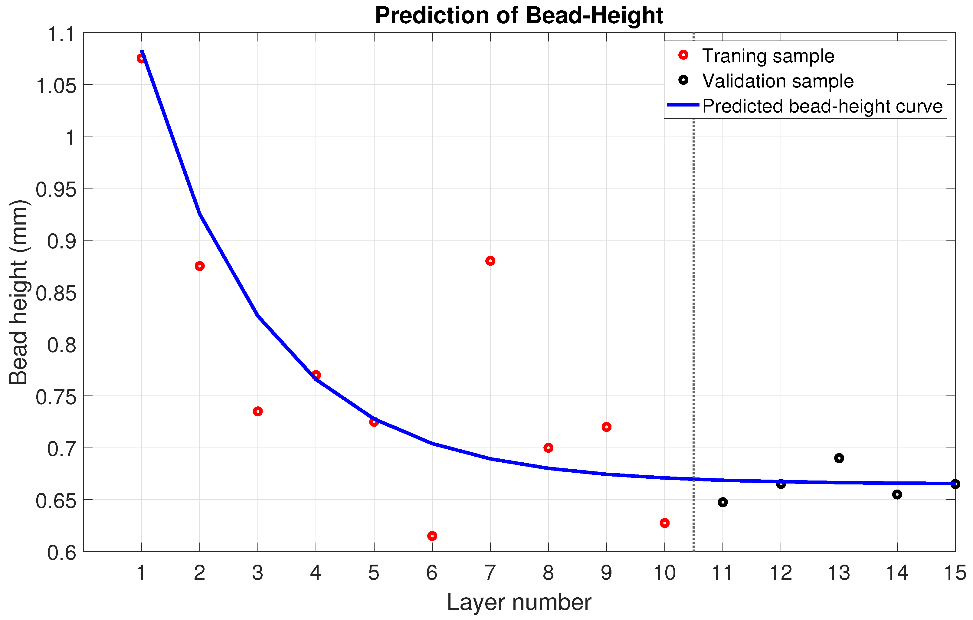
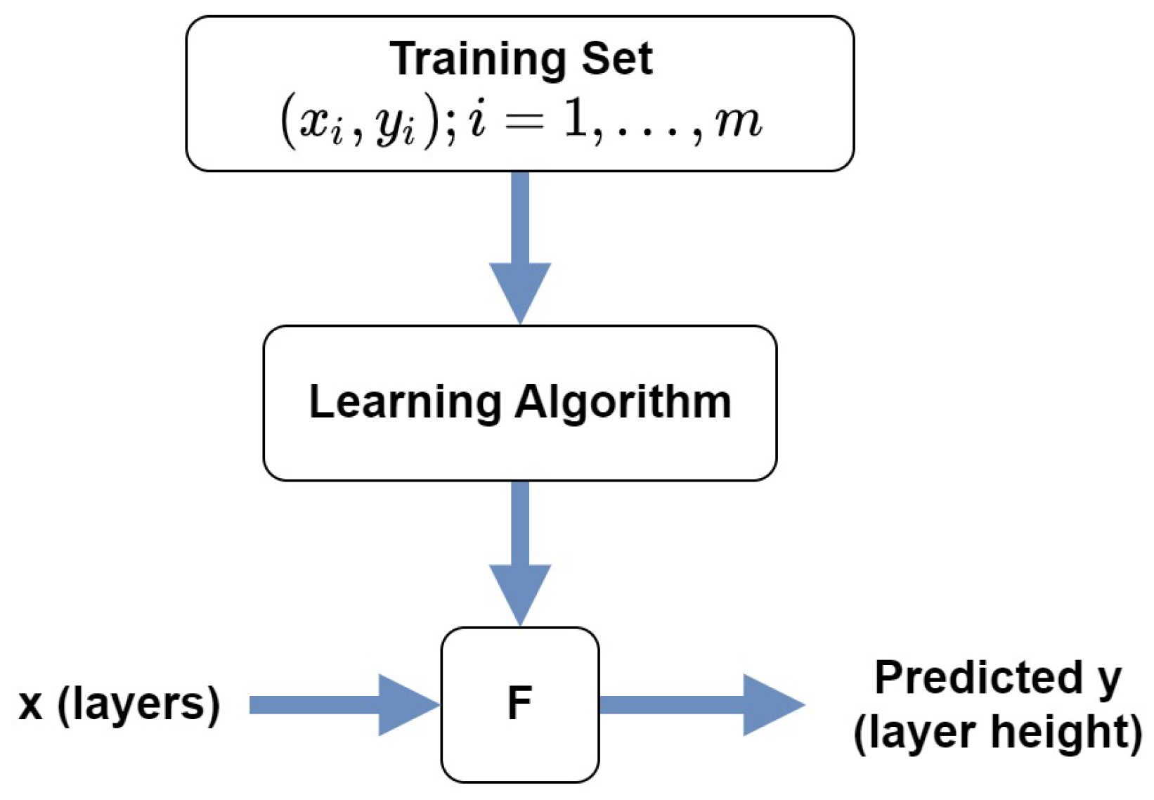
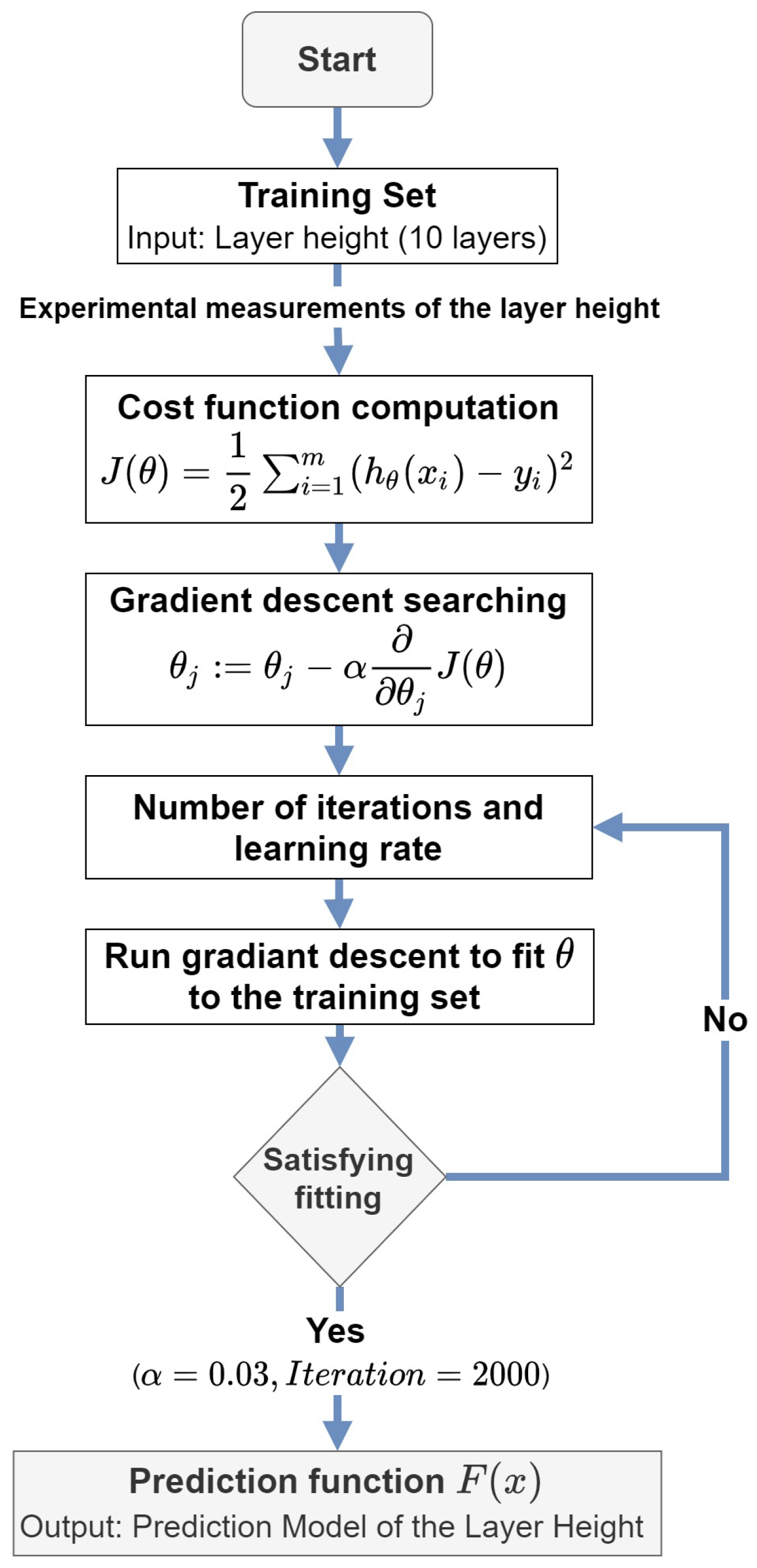
3.1. Bead Height Prediction Model

The prediction algorithm begins by creating a dataset to store training examples ($x_i,y_i$), $i=1$ to $m,m=$ final layer. $x_i$ is the input variable (number of layers) known as input features, and $y_i$ is the output variable (layer height) that needs to be predicted, also called the target variable.

The output of the regression is a prediction function $F\left(x\right)$. The function relates the evolution of the bead height over layers. The algorithm is implemented in Python and is composed of the following steps: First, a mapping function is created to represent a decreasing concave up function trend: $a\ast x^b+c$; a and $c>0$; $b<0$; a is the vertical stretch of the function; b is the rate of decay of the function and c the horizontal asymptote of the function. The mapping function displays the bead height evolution over layers. Then, the training set is plotted and the data linearized with a natural logarithm. After that, a linear regression algorithm is applied to fit the least-squares line to the natural logarithm plot (linearized model). Finally, the power decay function parameters are derived with which to compose the layer prediction function. The process of the bead height prediction is shown in Figure 4.

The linear model is represented with the following linear equation,

$$h\left(x\right)={\theta }_0+{\theta }_{1}x$$

(1)

where $\{{\theta }_j;j=0,1\}$ are unknown variables. Then, a cost function $J\left(\theta \right)$ is defined as follows:

$$J\left(\theta \right)={\displaystyle \frac{1}{2}}\sum _{i=1}^m{(h\left(x_i\right)-y_i)}^2$$

(2)

where $\{x_i,y_i;i=1,\dots ,m\}$. After that, $\theta$ is chosen so that the cost function $J\left(\theta \right)$ is minimized. A search algorithm called gradient descent is applied.

$${\theta }_j:={\theta }_j-\alpha {\displaystyle \frac{\partial }{\partial {\theta }_j}}J\left(\theta \right)$$

(3)

Note that this update is performed simultaneously for all values of $j=0,\dots ,n$, and n is the number of unknown variables. In this work, the learning rate ($\alpha$) technique is used; such that when the learning rate is decreased to zero, the regression algorithm converges to the global minimum rather than oscillating around the minimum. Tuning experiments will help to detect a reasonable learning-rate value. The partial derivative of $J\left(\theta \right)$ gives the least-mean-squares (LMS) update, which is also known as the Widrow–Hoff learning rule, and it is defined as follows:

$${\theta }_j:={\theta }_j+\alpha \sum _{i=1}^m(y_i-h_{\theta }\left(x_i\right))x_{i,j}\forall j$$

(4)

Finally, a number of iteration and learning rates were selected to converge to the best values of gradient descents. If the prediction output is not good, either the learning rate and the number of iterations are modified or the mapping function parameters are changed. The prediction process is summarized in the flowchart shown in Figure 5. In this work, the number of iterations ranges from 1500 to 2000, with a 0.03 learning rate.

3.2. Neural Network Prediction

In this paper, the neural network technique is used to study the correlations between the dispositional first-order parameters (laser power, wire feed rate and travel speed) and bead geometrical measurements (height and width) in the LWAM process. The Levenberg–Marquardt algorithm (LM) is used to train the neural network and solve the optimization problem [43].

The LM algorithm is designed to work specifically with loss functions that take the form of a sum of squared errors. It works without computing the exact Hessian matrix. Instead, it works with the gradient vector and the Jacobian matrix [44]. For the paper self-consistency, the LM algorithm computation is briefly discussed in this subsection.

Let us consider the following loss function which takes the form of a sum of squared errors,

$$f=\sum _{i=1}^m{e}_i^2$$

(5)

where m is the number of training samples. Then let’s define the Jacobian matrix of the loss function with respect to the parameters,

$$J_{i,j}={\displaystyle \frac{\partial e_i}{\partial w_j}},i=1,\dots ,m,j=1,\dots ,n$$

(6)

where m is the number of samples in the data set and n is the number of parameters in the neural network. Now, we can compute the gradient vector of the loss function as,

$$\nabla f=2J^T·e$$

(7)

where e is the vector of all error terms. Then, we can approximate the Hessian matrix with the following expression,

$$H_f\approx 2J^T·J+\lambda I$$

(8)

where $\lambda$ is a damping factor that ensures the positiveness of the Hessian and I is the identity matrix. Finally, The next expression defines the parameters improvement process with the Levenberg–Marquardt algorithm,

$$w_{(i+1)}=w_i-{(J_i^T·J_i+{\lambda }_{i}I)}^{-1}·(2J_i^T·e^{})$$

(9)

for $i=0,1,\dots ,m$, were w is the parameters vector. The parameter $\lambda$ is initialized to be large so that the first updates are small steps in the gradient descent direction. If any iteration results in a fail, then $\lambda$ is increased by some factor. As we will see in the following, this relatively simple method gave satisfying results for finding the relations between the input parameters and bead geometries.

4. Experimental Results and Discussion

Experimental test campaigns were carried out on the laser platform at Institut de Soudure. Tests were run by a robotized laser wire-feed system. An ABB 7-axis poly-articulated robot was used to provide the kinematics of the process. A fibre laser source, IPG Photonics, of 10 kW was used as the heat source. The system also used a CoaxPrinter laser processing head to deliver the laser beam and the filler wire to the processing zone. Figure 6 shows the actual LWAM system setup.

To perform the experiments, Grasshopper was used to create the physical part specifications (bead size, layer height, pattern, etc.). A generative algorithm was implemented and converted to robot programs using the HAL framework. In the experiment, a hollow wall of 150 mm × 50 mm was deposited and the complete deposition path was performed in generative algorithms.

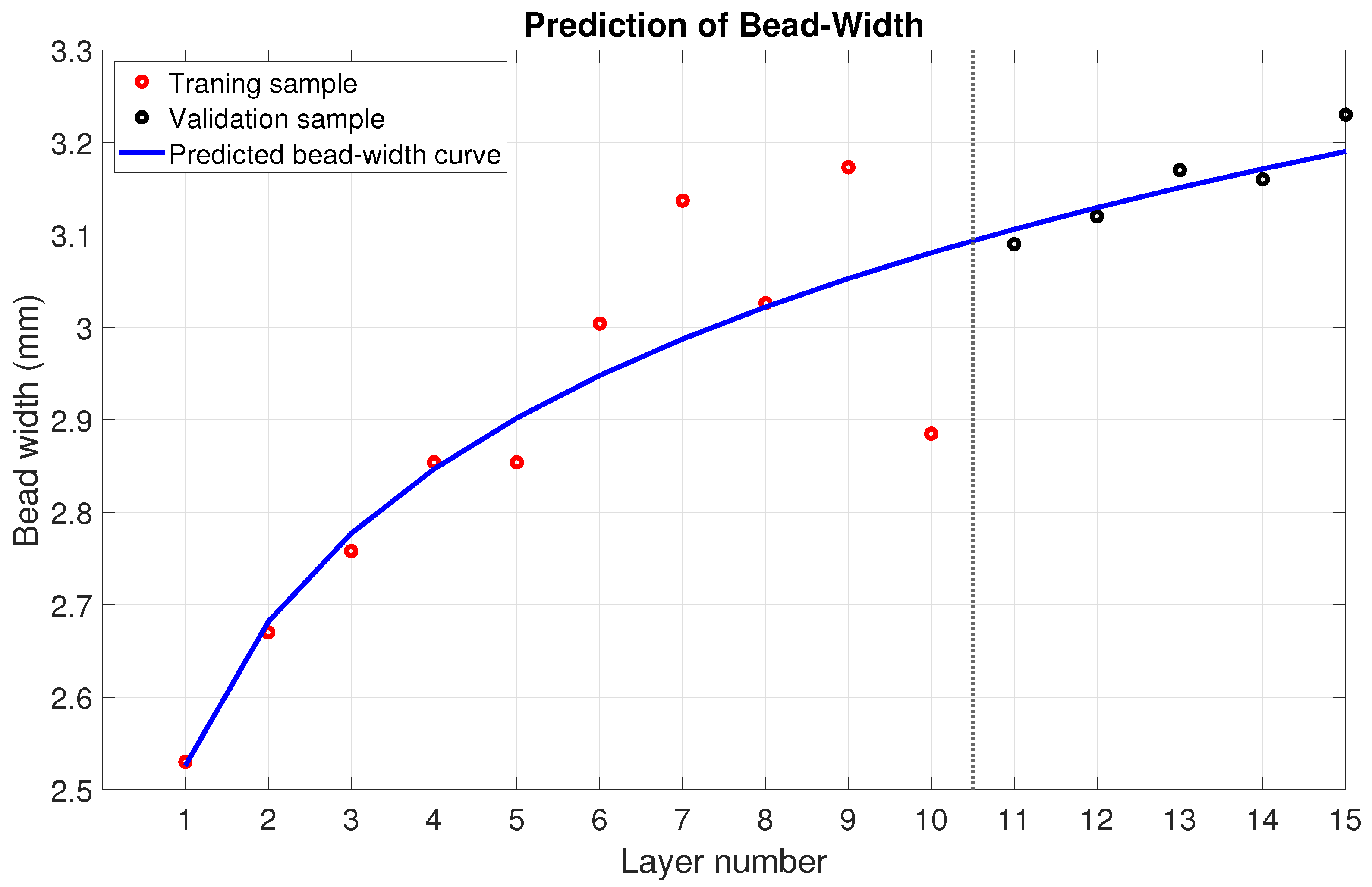
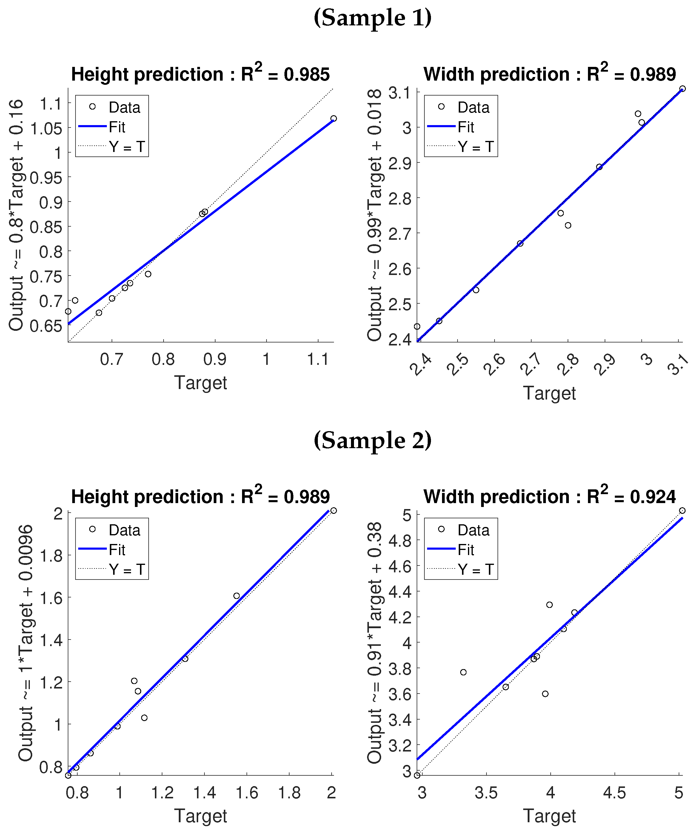
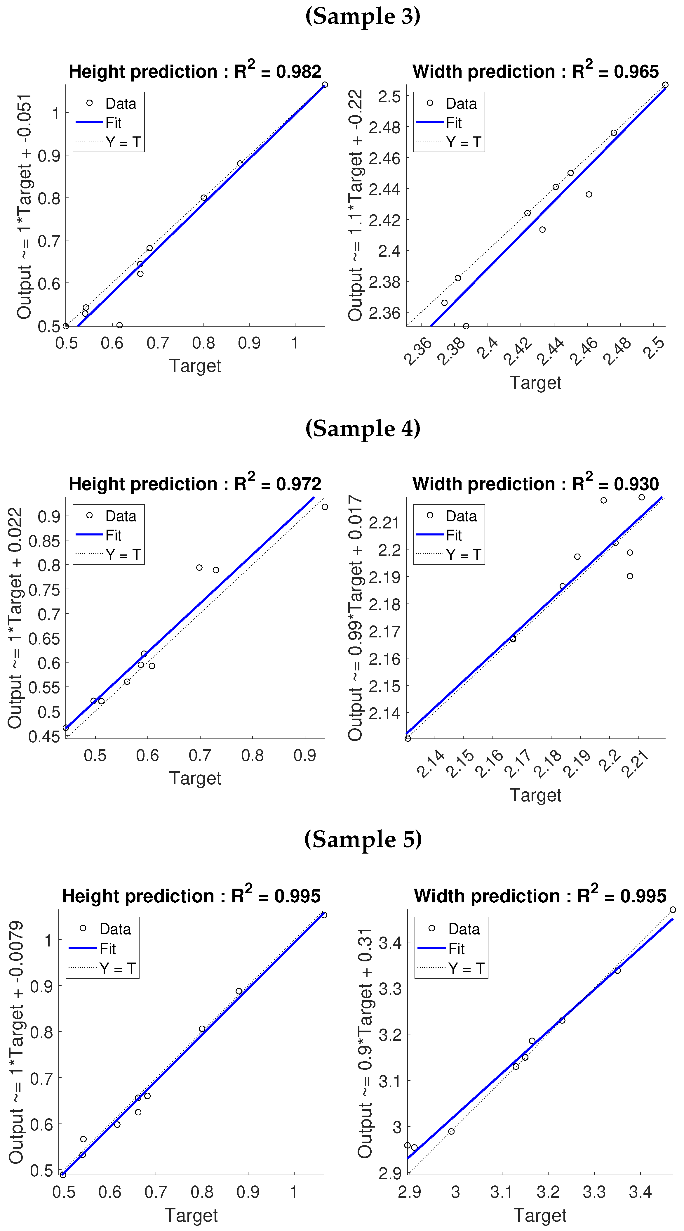
4.1. Bead Geometry Prediction

To test the prediction algorithm proposed in Section 3.1, a hollow wall of dimension 150 mm × 50 mm with 15 layers was deposited using the following process parameters: laser power $=1.4$ kW, wire-feed rate $=1.4$ m/min, and travel speed of robot $=0.45$ m/min. These initial process parameters were chosen to achieve a stable, uniform, and homogeneous final part, as shown in Figure 7.

Figure 8 and Figure 9 show the results of the prediction model height and width respectively. The figures show the prediction results for both the training data set (layers 1 to 10—red circle) and the prediction data set (layers 11 to 15—black circle).

It is worth noting that the plot of the training set in Figure 8 shows a power decay trend in height across layers. This observed trend is the so-called self-regulation mechanism of the layer height, and it has been discussed by Simone Donadello et al. in [25].

In Figure 10, the bead-width-over-bead-height ratio across layers is plotted. From this experimental result a logarithmic increase can be observed for each layer. In the observation, the width-to-height ratio increases significantly during the first layers before reaching a threshold around layer 10.

Interestingly, the prediction ratio, shown in Figure 10, indicates that the bead width’s increasing ratio is more significant compared with bead height change over layers. The physical phenomenon observed, here, is due to the conduction of heat resulting from the laser-matter interaction. When the wire is irradiated by the laser beam, the energy absorbed by the wire leads to creating molten pools and its deposition on the substrate. As the beads are added layer by layer, the heat source “moves away” from the substrate. The consequence is a decrease in the volume of material allowing the transfer of heat. This leads to an increase in the flux density, which inevitably leads to local heating, a modification of the local properties of the metal, and the wetting of the deposit, among other things. The spread of layers becomes important with the increase of bead widths and the decrease of the bead height. It is observed that this phenomenon stabilizes after a number of deposited layers, as shown Figure 11.

4.2. First-Order Deposition Parameters

To investigate the effectiveness of predictive models using neural network (discussed in Section 3.2), several experiments with three deposition parameters were carried out. As mentioned before, these parameters are laser power (P), wire feed rate (F), and travel speed (V), as presented in

Table 1. First-order deposition parameters.

Test Trial	P (kW)	F (m/min)	V (m/min)
Sample 1	1.6	0.6	2.0
Sample 2	1.6	0.3	2.2
Sample 3	2.0	0.9	2.2
Sample 4	1.6	1.2	2.2
Sample 5	1.4	1.4	0.45

. The choices for each of these five sets of parameters result from a test campaign for the development of the process with a wire of 1.2 mm diameter in Inconel^® 718 [45]. These five sets of parameters frame the stability domain of the process, i.e., they allow stable deposition with different bead morphologies, which is the parameter of interest for our study. Figure 12 shows different bead geometry samples for each parameter variation in the experimental design and for each sample, 10 deposition layers were measured (70% training data, 15% validation data and 15% as testing data).

In this study, the Levenberg–Marquardt algorithm (LM) was used to study the influence of the deposition parameters (P, F, V) on bead geometries (height and width). The main parameters for LM are the number of hidden layers and nodes. To obtain a good predictive performance a single hidden layer was chosen, with a size of 10 nodes (for more details see e.g., [7]). Additionally, other parameters were also determined by trial and error using 100 iterations for each sample. Figure 13 graphically illustrates a correlation between the measured height and the width predicted by the LM approach for the different deposition parameters. As the figure shows, the points are scattered around the fit line (represents measured bead geometry), which indicates the correlation between the model output values and the actual values. The value of $R^2$ reflects the correlation between the model prediction ($y^p$) and the corresponding target ($y^e$). The value of $R^2$ ranges from zero to one, and if $R^2$ is equal to one, it means a perfect correlation, and it can be computed as follows:

$$R^2=1-{\displaystyle \frac{{\sum }_{i=1}^n{[y_i^p-y_i^e]}^2}{{\sum }_{i=1}^n{[y_i^p-y^m]}^2}},y^m={\displaystyle \frac{1}{n}}\sum _{i=1}^n{y}_i^p$$

(10)

where n is the number of the experimental data.

To evaluate the accuracy of the prediction model obtained for each sample, we also computed RMSE, MAE, MAPE. The prediction accuracy of the regression model was judged excellent for RMSE, MAE and MAPE, being close to 0.

RMSE is computed to measure the standard deviation of residuals.

$$\mathrm{RMSE}=\sqrt{{\displaystyle \frac{1}{n}}\sum _{i=1}^n{(y_i^e-y_i^p)}^2}$$

(11)

MAE is the average of the absolute difference between $y^e$ and $y^p$ values in the data-set.

$$\mathrm{MAE}={\displaystyle \frac{1}{n}}\sum _{i=1}^n|y_i^e-y_i^p|$$

(12)

MAPE is the representation of MAE as a percentage.

$$\mathrm{MAPE}={\displaystyle \frac{1}{n}}\sum _{i=1}^n{\displaystyle \frac{|y_i^e-y_i^p|}{y_i^e}}\ast 100\%$$

(13)

Table 2. Model performance for different samples.

Sample	RMSE		${\mathit{R}}^2$		MAE		MAPE
	Height	Width	Height	Width	Height	Width	Height	Width
1	0.0361	0.0337	0.9847	0.9894	0.0282	0.0082	2.8151%	0.8235%
2	0.0580	0.2053	0.9888	0.9242	0.0291	0.0301	2.9098%	3.0145%
3	0.0392	0.0154	0.9818	0.9652	0.0345	0.0037	3.4547%	0.3704%
4	0.0388	0.0094	0.9717	0.9300	0.0408	0.0030	4.0777%	0.2951%
5	0.0176	0.0258	0.9954	0.9947	0.0232	0.0047	2.3192%	0.4720%

compares the bead geometry prediction performance of different samples for the LWAM process.

The results from Table 2 shows that the best test trial reported is sample 5, as it shows good values of prediction accuracy measurements both for bead width and height. This good result was obtained due to the smooth thickness transition across layers and the good distribution of the layer thicknesses by using a high wire-feed rate with low power and travel speed compared with the other measured samples.

On the other hand, the worst performance reported is Sample 2, which shows the worst values of prediction accuracy measurements. It is noted that Sample 2 has the highest RMSE, MAE and MAPE; however, $R^2$ was good. This is due to the fact that $R^2$ gives an estimate of the strength of the relationship between $y^e$ and the prediction curve $F\left(x\right)$, the value reported for this test does not provide a formal explanation of the fitting. Another explanation of the value obtained obtains from the distribution of the $y^e$ in sample 2 that shows a similar trend with the prediction curve, which does not fit the $y^e$ values. These prediction results indicated that having a high laser power and travel speed with a low wire-feed rate will lead to bad results on the final bead geometry.

Finally, these results are summarized in

Table 3. Influence of the deposition parameters.

	P	V	F
Acceptable bead Prediction	Low	Low	High
Good layer Deposition	Low	Low	High

, which illustrates the influence of deposition parameters on both the prediction model and the bead geometry’s accuracy. It is worth mentioning that the designation “Acceptable bead prediction” in Table 3 takes the trend of the set of parameters with the best correlation coefficients (RMSE, $R^2$, MAE, MAPE). While the designation “Good layer deposition” refers to those experimental tests that showed process stability (no stuck wire, stable metal vapour plume, etc.) for a low laser power/travel speed coupling and a high wire-feed speed.

5. Conclusions

A bead geometry prediction model, in the LWAM process, was developed using a machine learning regression algorithm and neural network. The proposed algorithm predicted bead height, width and the ratio therebetween, and the results confirmed the profile’s trend toward stable deposition. The prediction model is flexible and can be adjusted to follow the trends of various layer-deposition behaviours.

The experimental results revealed that the developed machine learning model is capable of predicting the bead geometry of LWAM-deposited layers with acceptable error rates (i.e., 2∼4%). Several data samples have been also collected by a laser scanner to study the influence of different deposition parameters on the bead geometry. The prediction results of low power (P) and travel speed (V) with a high wire feed rate (F) showed better layer deposition and model prediction, as compared with other collected samples.

In summary, the following conclusions are drawn from this study:

• Regression algorithms can be used for prediction tasks related to the LWAM process, including for supervision tasks;
• There exists a power decay in correlating process parameters to bead thickness.
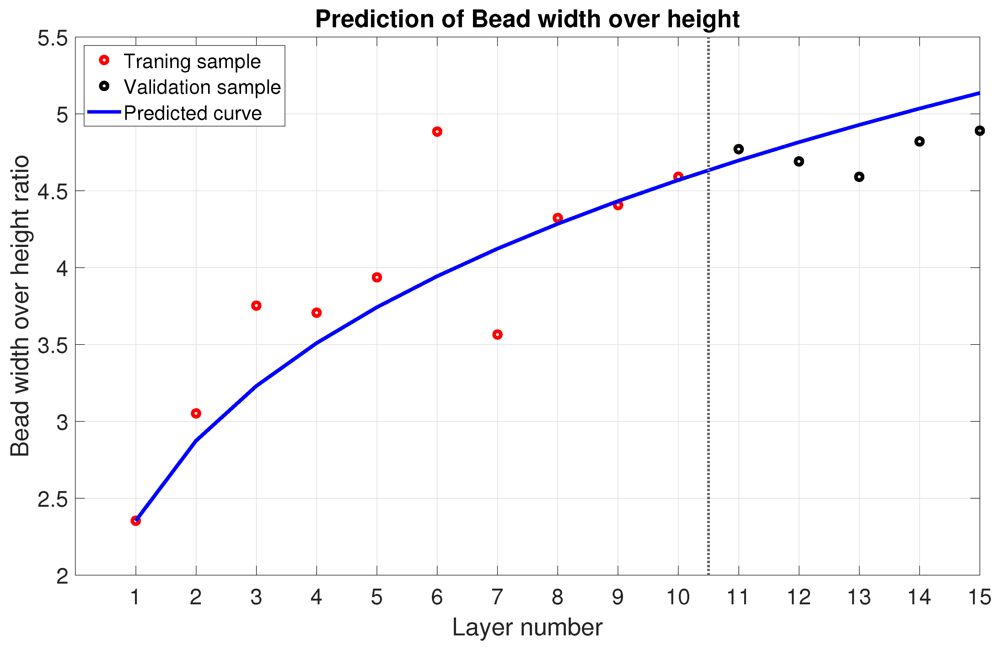
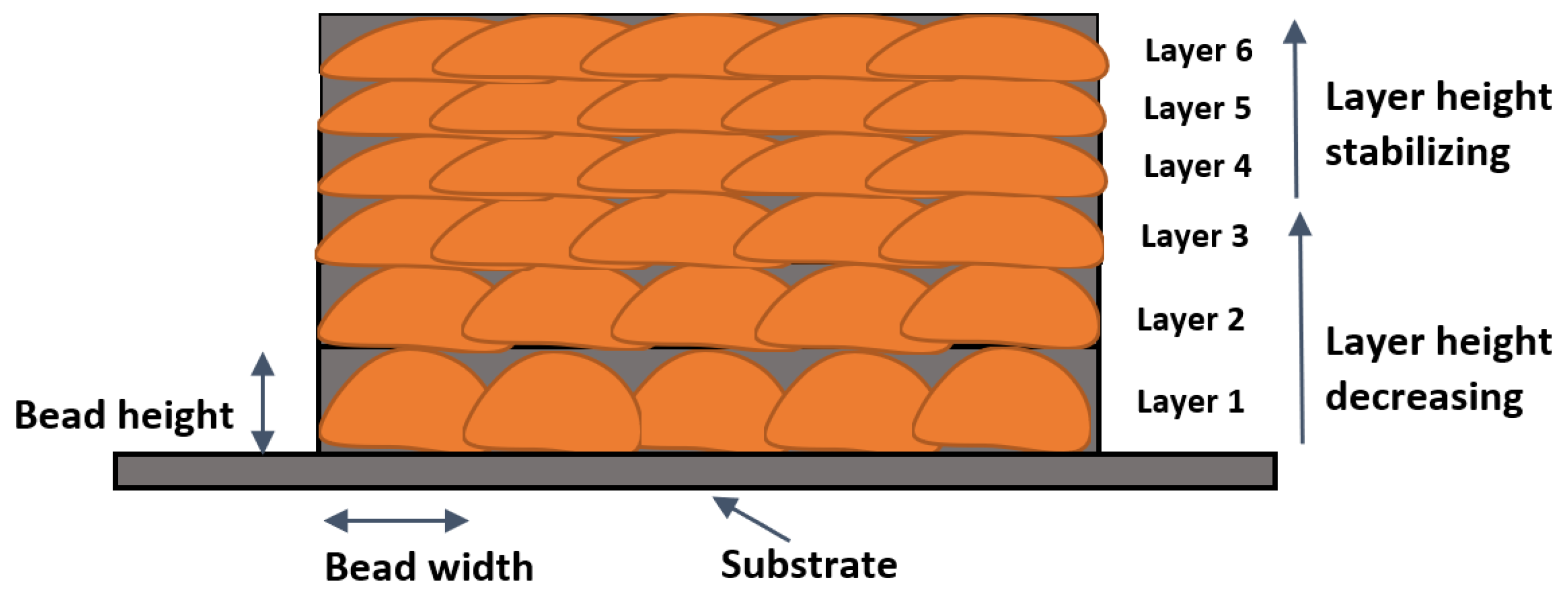
• The experimental results showed an increase of width-to-height ratio as a function of layer progression due to the heat conducted from the laser–matter interaction.
• Satisfying prediction models were obtained and could be used to predict the geometry of beads as part of LWAM control programming for horizontal and vertical robot movement.
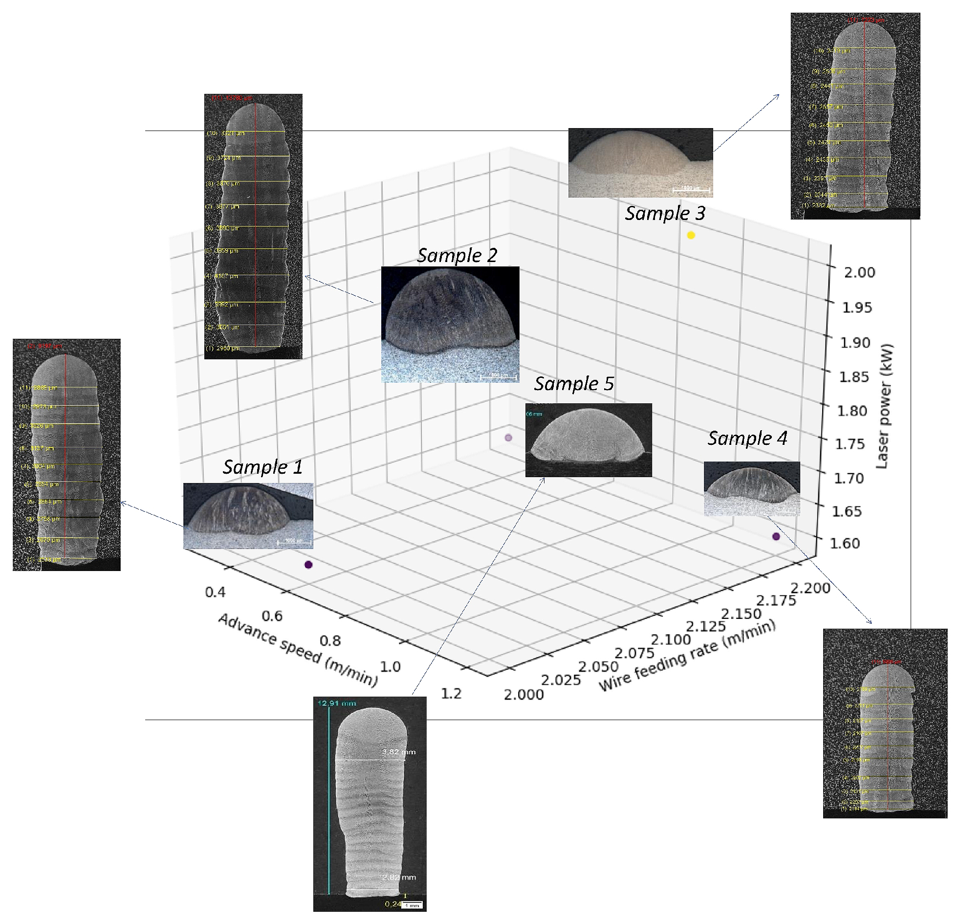
• In this case, acceptable bead prediction with good layer deposition was obtained when P, V, and F were $1.4$ kW, $1.4$ m/min, and $0.45$ m/min, respectively.

In the future, the prediction model will be used to develop a robust feedback control system that is able to adjust process parameters automatically for improving the surface quality and geometric accuracy in the LWAM process.

References

1. Shaqour, B.; Abuabiah, M.; Abdel-Fattah, S.; Juaidi, A.; Abdallah, R.; Abuzaina, W.; Qarout, M.; Verleije, B.; Cos, P. Gaining a better understanding of the extrusion process in fused filament fabrication 3D printing: A review. Int. J. Adv. Manuf. Technol. 2021, 114, 1279–1291. [Google Scholar] [CrossRef]
2. Zenou, M.; Grainger, L. Additive manufacturing of metallic materials. In Additive Manufacturing; Elsevier: Amsterdam, The Netherlands, 2018; pp. 53–103. [Google Scholar]
3. Ding, D.; Pan, Z.; Cuiuri, D.; Li, H. A multi-bead overlapping model for robotic wire and arc additive manufacturing (WAAM). Robot. Comput.-Integr. Manuf. 2015, 31, 101–110. [Google Scholar] [CrossRef] [Green Version]
4. Frostevarg, J. Comparison of three different arc modes for laser-arc hybrid welding steel. J. Laser Appl. 2016, 28, 022407. [Google Scholar] [CrossRef]
5. Brooks, H.; Molony, S. Design and evaluation of additively manufactured parts with three dimensional continuous fibre reinforcement. Mater. Des. 2016, 90, 276–283. [Google Scholar] [CrossRef] [Green Version]
6. Shamsaei, N.; Yadollahi, A.; Bian, L.; Thompson, S.M. An overview of Direct Laser Deposition for additive manufacturing; Part II: Mechanical behavior, process parameter optimization and control. Addit. Manuf. 2015, 8, 12–35. [Google Scholar] [CrossRef]
7. Xia, C.; Pan, Z.; Polden, J.; Li, H.; Xu, Y.; Chen, S. Modelling and prediction of surface roughness in wire arc additive manufacturing using machine learning. J. Intell. Manuf. 2021, 1–16. [Google Scholar] [CrossRef]
8. Muscato, G.; Spampinato, G.; Cantelli, L. A closed loop welding controller for a rapid manufacturing process. In Proceedings of the 2008 IEEE International Conference on Emerging Technologies and Factory Automation, Hamburg, Germany, 15–18 September 2008; pp. 1080–1083. [Google Scholar]
9. Ding, Y.; Warton, J.; Kovacevic, R. Development of sensing and control system for robotized laser-based direct metal addition system. Addit. Manuf. 2016, 10, 24–35. [Google Scholar] [CrossRef] [Green Version]
10. Bi, G.; Gasser, A.; Wissenbach, K.; Drenker, A.; Poprawe, R. Characterization of the process control for the direct laser metallic powder deposition. Surf. Coat. Technol. 2006, 201, 2676–2683. [Google Scholar] [CrossRef]
11. Song, L.; Bagavath-Singh, V.; Dutta, B.; Mazumder, J. Control of melt pool temperature and deposition height during direct metal deposition process. Int. J. Adv. Manuf. Technol. 2012, 58, 247–256. [Google Scholar] [CrossRef]
12. Meriaudeau, F.; Truchetet, F. Control and optimization of the laser cladding process using matrix cameras and image processing. J. Laser Appl. 1996, 8, 317–324. [Google Scholar] [CrossRef]
13. Toyserkani, E.; Khajepour, A. A mechatronics approach to laser powder deposition process. Mechatronics 2006, 16, 631–641. [Google Scholar] [CrossRef]
14. Hu, D.; Kovacevic, R. Sensing, modeling and control for laser-based additive manufacturing. Int. J. Mach. Tools Manuf. 2003, 43, 51–60. [Google Scholar] [CrossRef]
15. Koch, J.; Mazumder, J. Apparatus and Methods for Monitoring and Controlling Multi-Layer Laser Cladding. U.S. Patent 6,122,564, 19 September 2000. [Google Scholar]
16. Fox, M.D.; Hand, D.P.; Su, D.; Jones, J.D.; Morgan, S.A.; McLean, M.A.; Steen, W.M. Optical sensor to monitor and control temperature and build height of the laser direct-casting process. Appl. Opt. 1998, 37, 8429–8433. [Google Scholar] [CrossRef] [PubMed]
17. Zhang, Y.M.; Yang, Y.P.; Zhang, W.; Na, S.J. Advanced welding manufacturing: A brief analysis and review of challenges and solutions. J. Manuf. Sci. Eng. 2020, 142, 110816. [Google Scholar] [CrossRef]
18. Ma, M.; Wang, Z.; Gao, M.; Zeng, X. Layer thickness dependence of performance in high-power selective laser melting of 1Cr18Ni9Ti stainless steel. J. Mater. Process. Technol. 2015, 215, 142–150. [Google Scholar] [CrossRef]
19. Yadroitsev, I.; Smurov, I. Selective laser melting technology: From the single laser melted track stability to 3D parts of complex shape. Phys. Procedia 2010, 5, 551–560. [Google Scholar] [CrossRef] [Green Version]
20. Guan, K.; Wang, Z.; Gao, M.; Li, X.; Zeng, X. Effects of processing parameters on tensile properties of selective laser melted 304 stainless steel. Mater. Des. 2013, 50, 581–586. [Google Scholar] [CrossRef]
21. Averyanova, M.; Cicala, E.; Bertrand, P.; Grevey, D. Experimental design approach to optimize selective laser melting of martensitic 17-4 PH powder: Part I–single laser tracks and first layer. Rapid Prototyp. J. 2012, 18, 28–37. [Google Scholar] [CrossRef]
22. Dai, K.; Shaw, L. Parametric studies of multi-material laser densification. Mater. Sci. Eng. A 2006, 430, 221–229. [Google Scholar] [CrossRef]
23. Mbodj, N.G.; Plapper, P. Bead Width Prediction in Laser Wire Additive Manufacturing Process. In Recent Advances in Manufacturing Engineering and Processes; Springer: Berlin, Germany, 2022; pp. 33–40. [Google Scholar]
24. Zhu, G.; Li, D.; Zhang, A.; Pi, G.; Tang, Y. The influence of laser and powder defocusing characteristics on the surface quality in laser direct metal deposition. Opt. Laser Technol. 2012, 44, 349–356. [Google Scholar] [CrossRef]
25. Donadello, S.; Motta, M.; Demir, A.G.; Previtali, B. Monitoring of laser metal deposition height by means of coaxial laser triangulation. Opt. Lasers Eng. 2019, 112, 136–144. [Google Scholar] [CrossRef] [Green Version]
26. Simeone, O. A brief introduction to machine learning for engineers. Found. Trends Signal Process. 2018, 12, 200–431. [Google Scholar] [CrossRef]
27. Parisi, G.I.; Kemker, R.; Part, J.L.; Kanan, C.; Wermter, S. Continual lifelong learning with neural networks: A review. Neural Netw. 2019, 113, 54–71. [Google Scholar] [CrossRef]
28. Khatir, S.; Tiachacht, S.; Le Thanh, C.; Ghandourah, E.; Mirjalili, S.; Wahab, M.A. An improved Artificial Neural Network using Arithmetic Optimization Algorithm for damage assessment in FGM composite plates. Compos. Struct. 2021, 273, 114287. [Google Scholar] [CrossRef]
29. Tran-Ngoc, H.; Khatir, S.; Ho-Khac, H.; De Roeck, G.; Bui-Tien, T.; Wahab, M.A. Efficient Artificial neural networks based on a hybrid metaheuristic optimization algorithm for damage detection in laminated composite structures. Compos. Struct. 2021, 262, 113339. [Google Scholar] [CrossRef]
30. Zenzen, R.; Khatir, S.; Belaidi, I.; Le Thanh, C.; Wahab, M.A. A modified transmissibility indicator and Artificial Neural Network for damage identification and quantification in laminated composite structures. Compos. Struct. 2020, 248, 112497. [Google Scholar] [CrossRef]
31. Xiong, J.; Zhang, G.; Hu, J.; Wu, L. Bead geometry prediction for robotic GMAW-based rapid manufacturing through a neural network and a second-order regression analysis. J. Intell. Manuf. 2014, 25, 157–163. [Google Scholar] [CrossRef]
32. Nagesh, D.; Datta, G. Genetic algorithm for optimization of welding variables for height to width ratio and application of ANN for prediction of bead geometry for TIG welding process. Appl. Soft Comput. 2010, 10, 897–907. [Google Scholar] [CrossRef]
33. Milhomme, S.; Lartigau, J.; Brugger, C.; Froustey, C. Bead geometry prediction using multiple linear regression analysis. Int. J. Adv. Manuf. Technol. 2021, 117, 607–620. [Google Scholar] [CrossRef]
34. Karmuhilan, M.; Kumarsood, A. Intelligent process model for bead geometry prediction in WAAM. Mater. Today Proc. 2018, 5, 24005–24013. [Google Scholar] [CrossRef]
35. Wacker, C.; Köhler, M.; David, M.; Aschersleben, F.; Gabriel, F.; Hensel, J.; Dilger, K.; Dröder, K. Geometry and Distortion Prediction of Multiple Layers for Wire Arc Additive Manufacturing with Artificial Neural Networks. Appl. Sci. 2021, 11, 4694. [Google Scholar] [CrossRef]
36. Ayed, A.; Bras, G.; Bernard, H.; Michaud, P.; Balcaen, Y.; Alexis, J. Study of Arc-wire and Laser-wire processes for the realization of Ti-6Al-4V alloy parts. MATEC Web Conf. EDP Sci. 2020, 321, 03002. [Google Scholar] [CrossRef]
37. Lim, S.; Buswell, R.A.; Valentine, P.J.; Piker, D.; Austin, S.A.; De Kestelier, X. Modelling curved-layered printing paths for fabricating large-scale construction components. Addit. Manuf. 2016, 12, 216–230. [Google Scholar] [CrossRef] [Green Version]
38. Nilsson, D. G-Code to RAPID Translator for Robot-Studio. Master’s Thesis, University West, Trollhattan, Sweden, 2016. [Google Scholar]
39. Schwartz, T. Extension of a visual programming language to support teaching and research on robotics applied to construction. In Rob|Arch 2012; Springer: Berlin, Germany, 2013; pp. 92–101. [Google Scholar]
40. Misra, D.; Sundararajan, V.; Wright, P.K. Zig-zag tool path generation for sculptured surface. In Geometric and Algorithmic Aspects of Computer-Aided Design and Manufacturing; American Mathematical Society: Piscataway, NJ, USA, 2005; p. 265. [Google Scholar]
41. Ren, K.; Chew, Y.; Liu, N.; Zhang, Y.; Fuh, J.; Bi, G. Integrated numerical modelling and deep learning for multi-layer cube deposition planning in laser aided additive manufacturing. Virtual Phys. Prototyp. 2021, 16, 318–332. [Google Scholar] [CrossRef]
42. Liu, F.; Wei, L.; Shi, S.; Wei, H. On the varieties of build features during multi-layer laser directed energy deposition. Addit. Manuf. 2020, 36, 101491. [Google Scholar] [CrossRef]
43. Ranganathan, A. The levenberg-marquardt algorithm. Tutoral LM Algorithm 2004, 11, 101–110. [Google Scholar]
44. Farber, R. CUDA Application Design and Development; Elsevier: Amsterdam, The Netherlands, 2011. [Google Scholar]
45. Cazic, I.; Zollinger, J.; Mathieu, S.; El Kandaoui, M.; Plapper, P.; Appolaire, B. New insights into the origin of fine equiaxed microstructures in additively manufactured Inconel 718. Scr. Mater. 2021, 195, 113740. [Google Scholar] [CrossRef]
Figure 1. Schematic diagram of the LWAM PRECITEC laser head with the optical path of the laser beam and injection of the filler metal.
Applsci 11 11949 g001
Figure 2. Flowchart diagram of the proposed approach for the LWAM system.
Applsci 11 11949 g002
Figure 3. (a) Single bead geometry measurements. (b) Layer deposition measurements.
Applsci 11 11949 g003
Figure 4. Bead height prediction process.
Applsci 11 11949 g004
Figure 5. Flowchart of the bead height prediction model.
Applsci 11 11949 g005
Figure 6. Experimental Setup of LWAM platform at Institut de Soudure.
Applsci 11 11949 g006
Figure 7. Experimental layers deposit; (a) front view, (b) side view.
Applsci 11 11949 g007
Figure 8. Result of the bead height prediction.
Applsci 11 11949 g008
Figure 9. Result of the bead width prediction.
Applsci 11 11949 g009
Figure 10. Bead width over height prediction.
Applsci 11 11949 g010
Figure 11. Schematic diagram of bead width and bead height for different deposited layers.
Applsci 11 11949 g011
Figure 12. Bead geometry samples.
Applsci 11 11949 g012
Figure 13. Regression plot for different samples prediction.
Applsci 11 11949 g013aApplsci 11 11949 g013b