
Assessment of Agricultural Water Requirements for Semi-Arid Areas: A Case Study of the Boufakrane River Watershed (Morocco)

 ,
,  , ,
, ,  and
and 
Abstract
:1. Introduction
- (a)
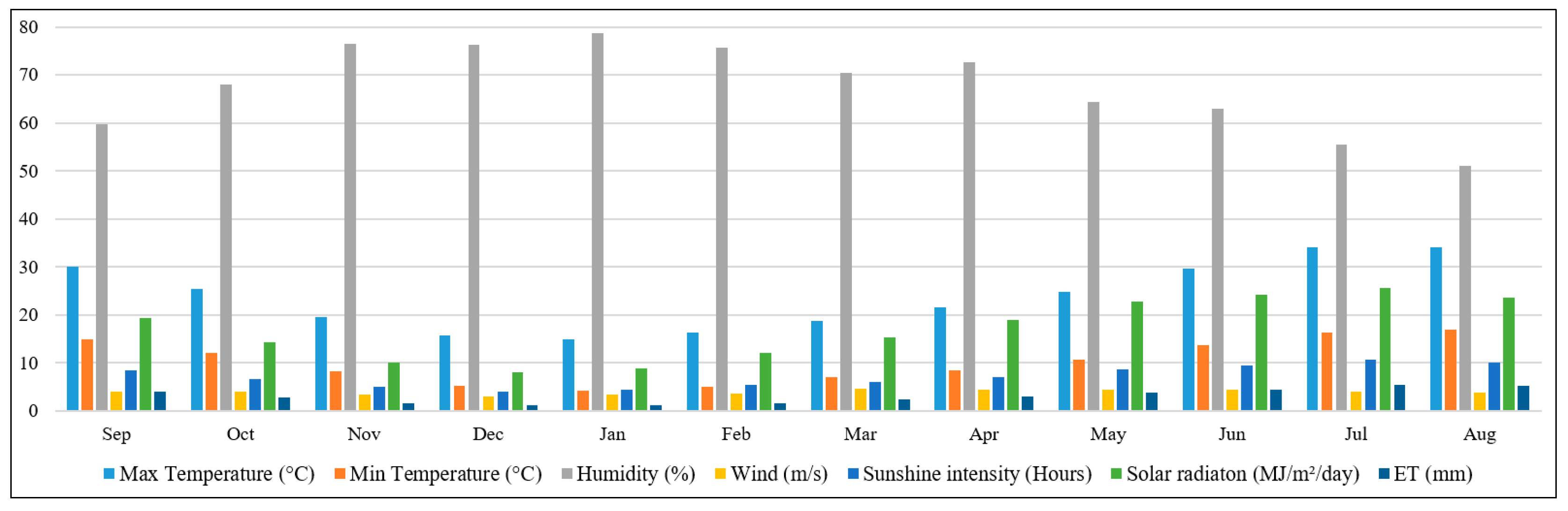
- Reference evapotranspiration (ET0): Collect climate data and choose the method for calculating ET0 for each 30 or 10 day period using the average climate data.
- (b)
- Crop coefficient (kc): Determine the timing of planting or sowing, the rate of crop development, the duration of crop development stages and the growing season. Choose the kc for a given crop plan and crop development stage under prevailing climatic conditions, and prepare a crop coefficient curve for each one.
- (c)
- Crop evapotranspiration (ETcrop): Calculate ETcrop for each 30- or 10-day period:
2. Materials and Methods
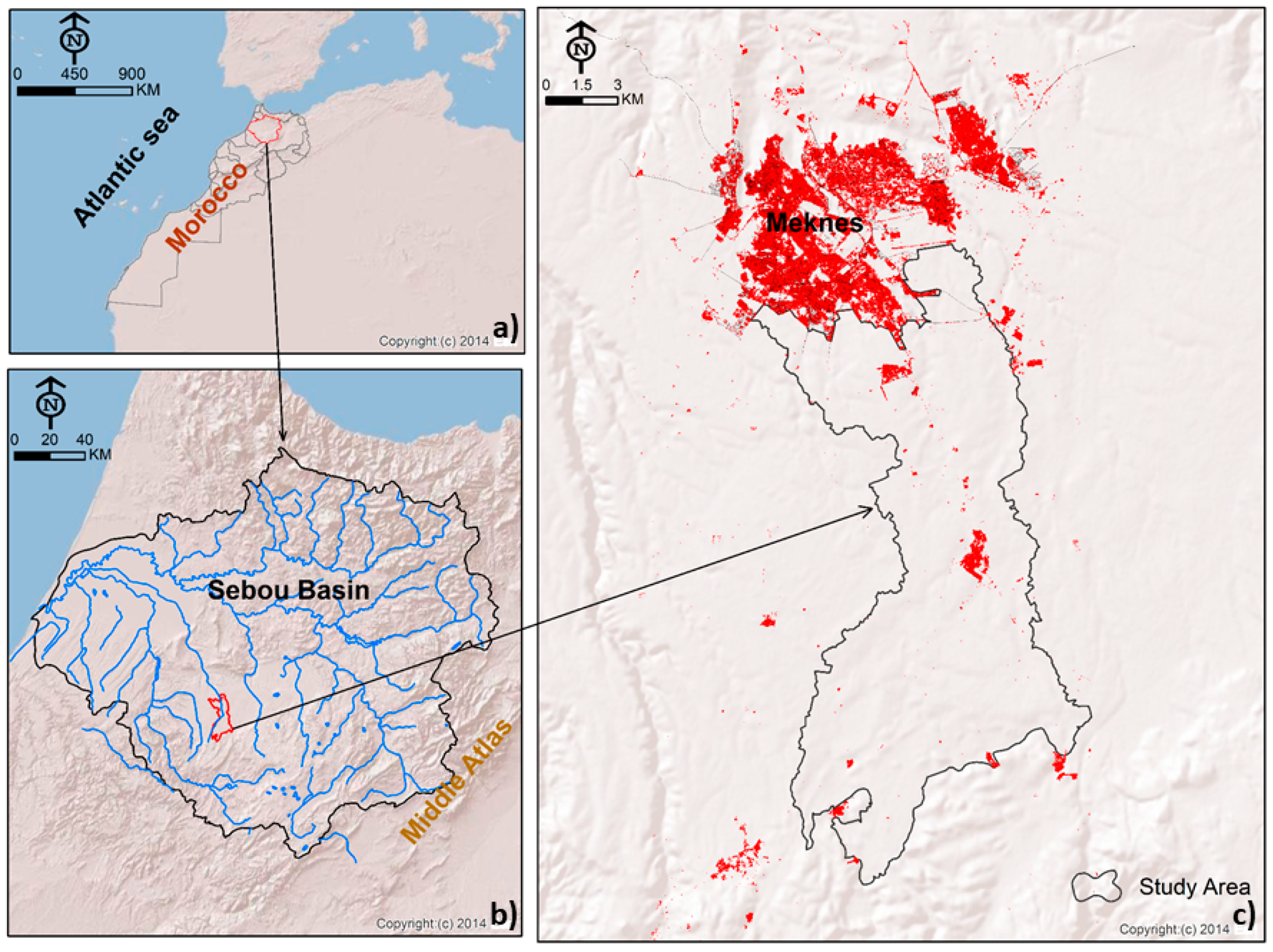
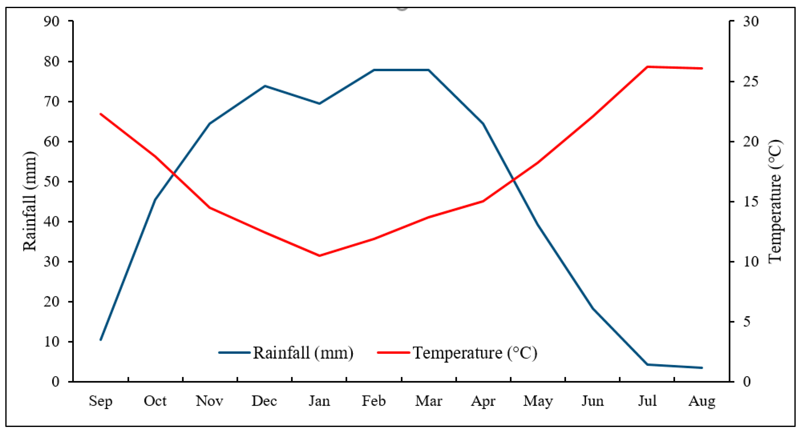
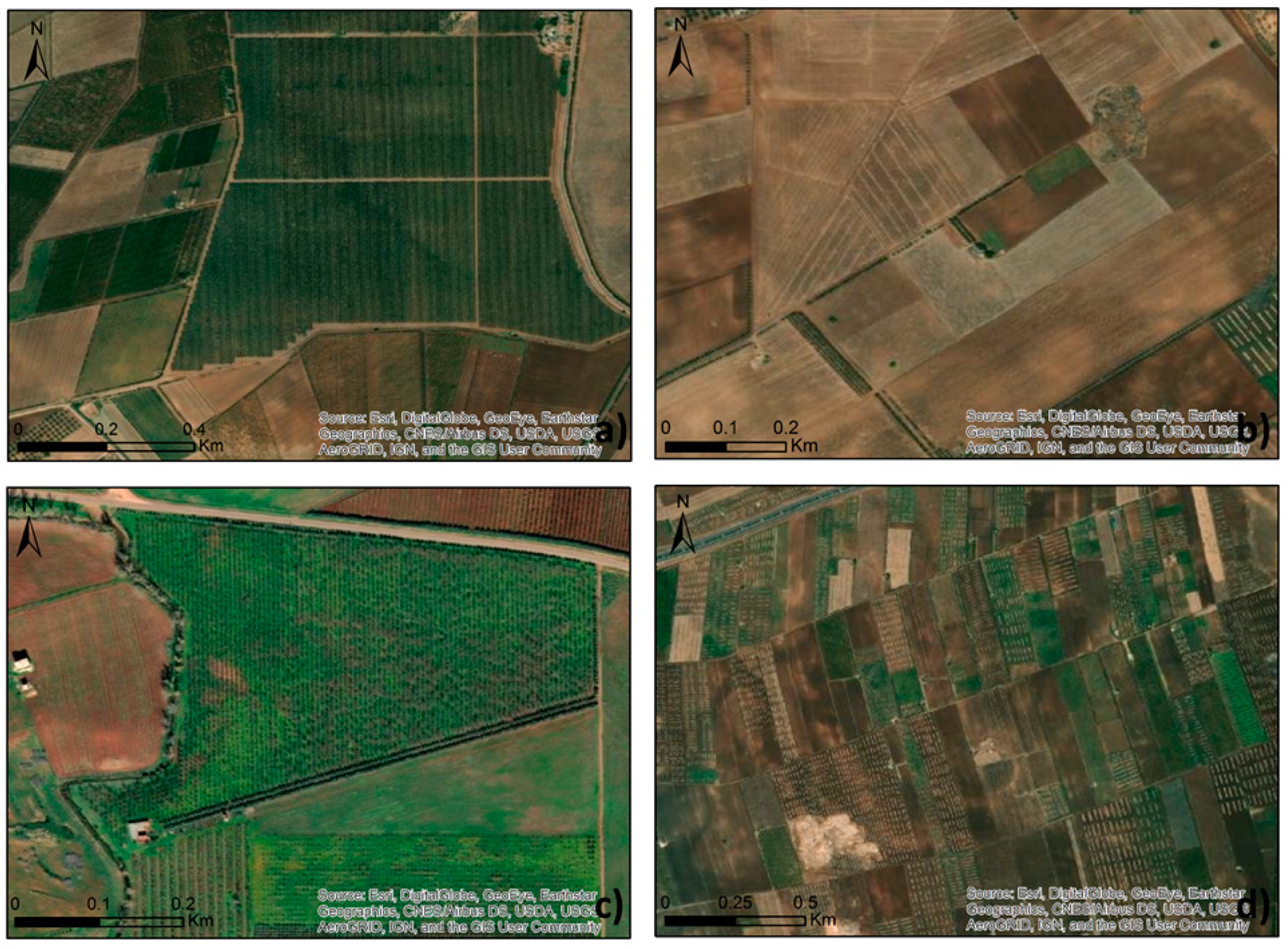
2.1. Study Area
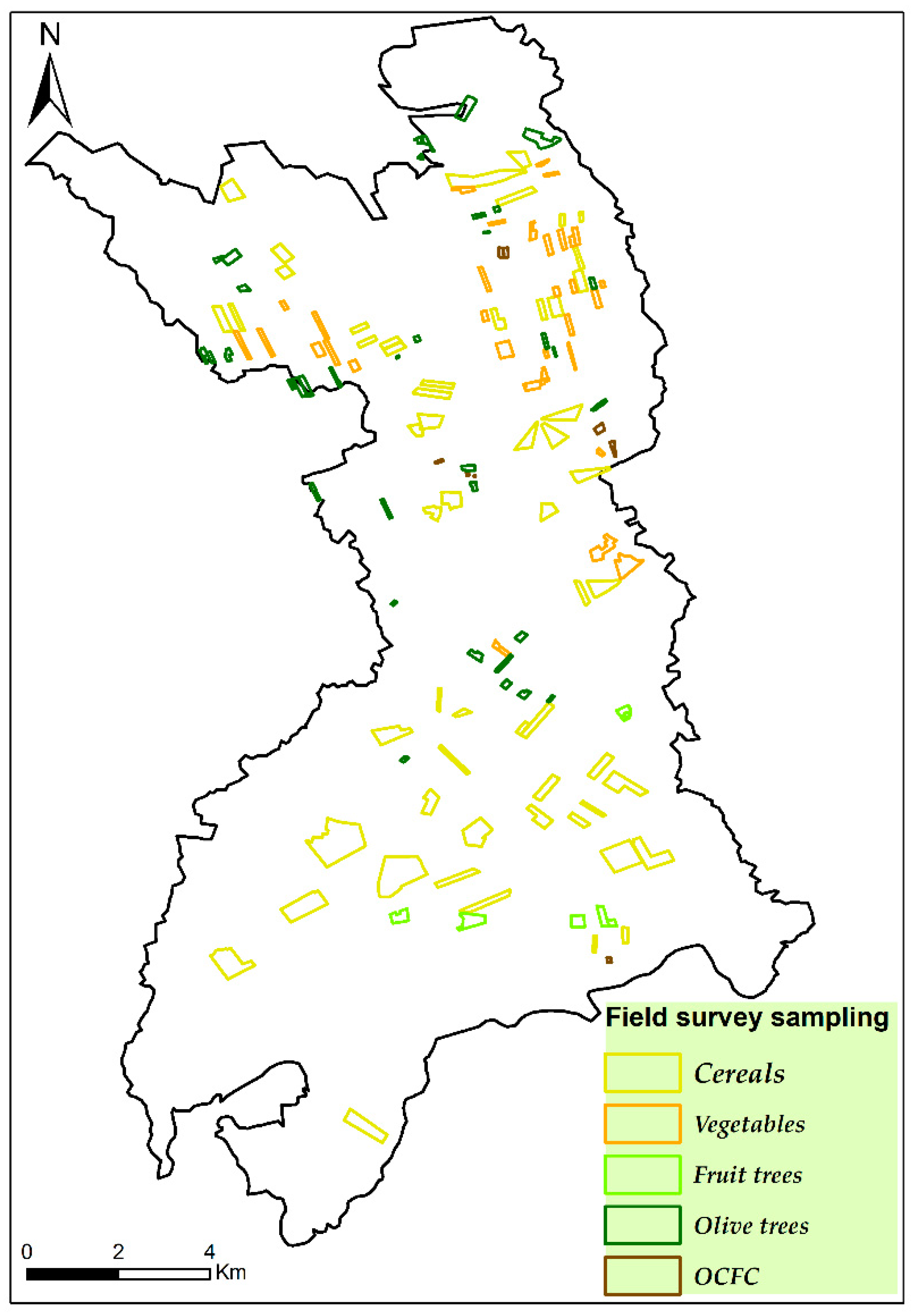
2.2. Data
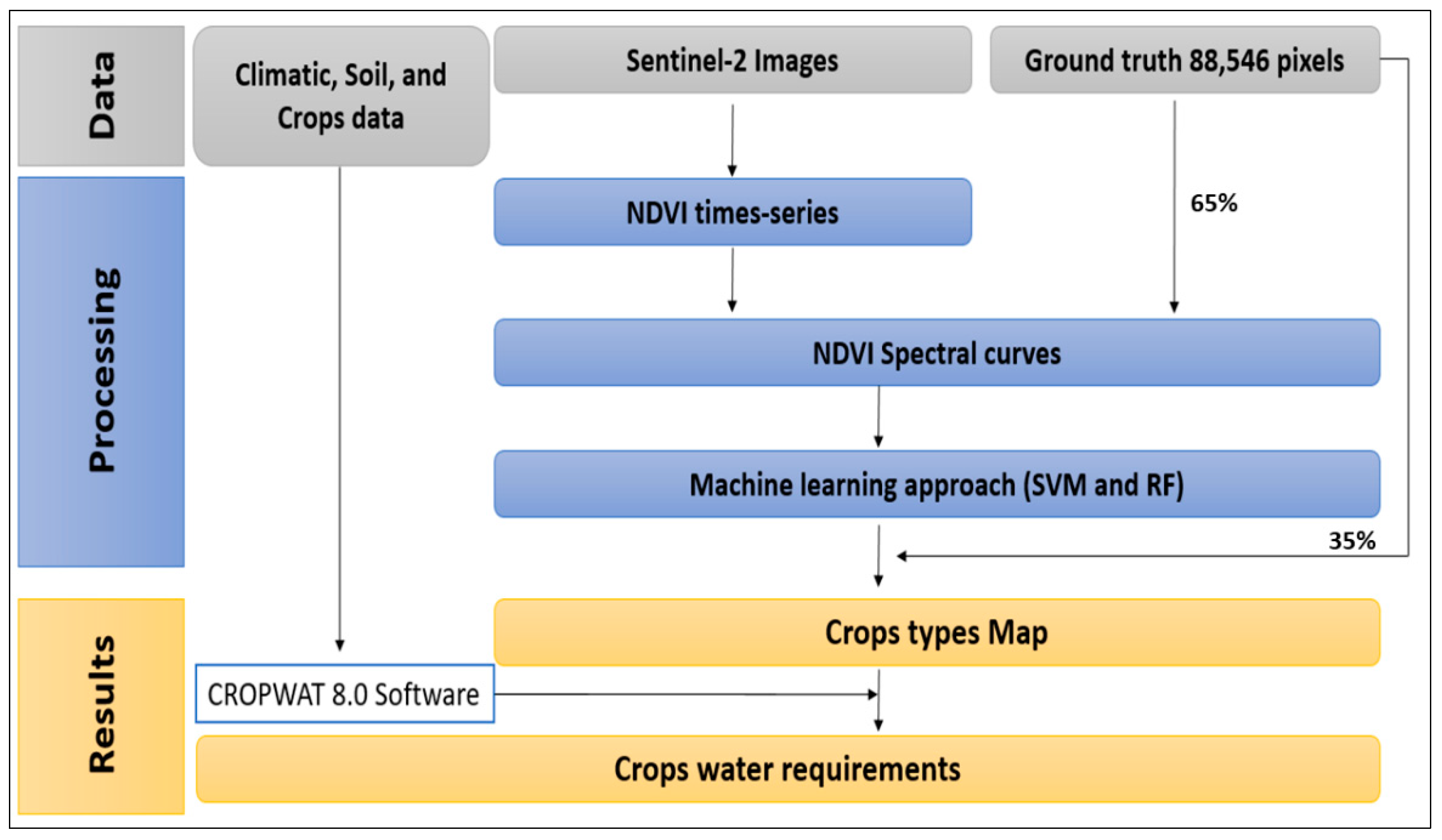
2.3. Methodolgy
2.4. Support Vector Machine (SVM)
2.5. Random Forest (RF) Classifier
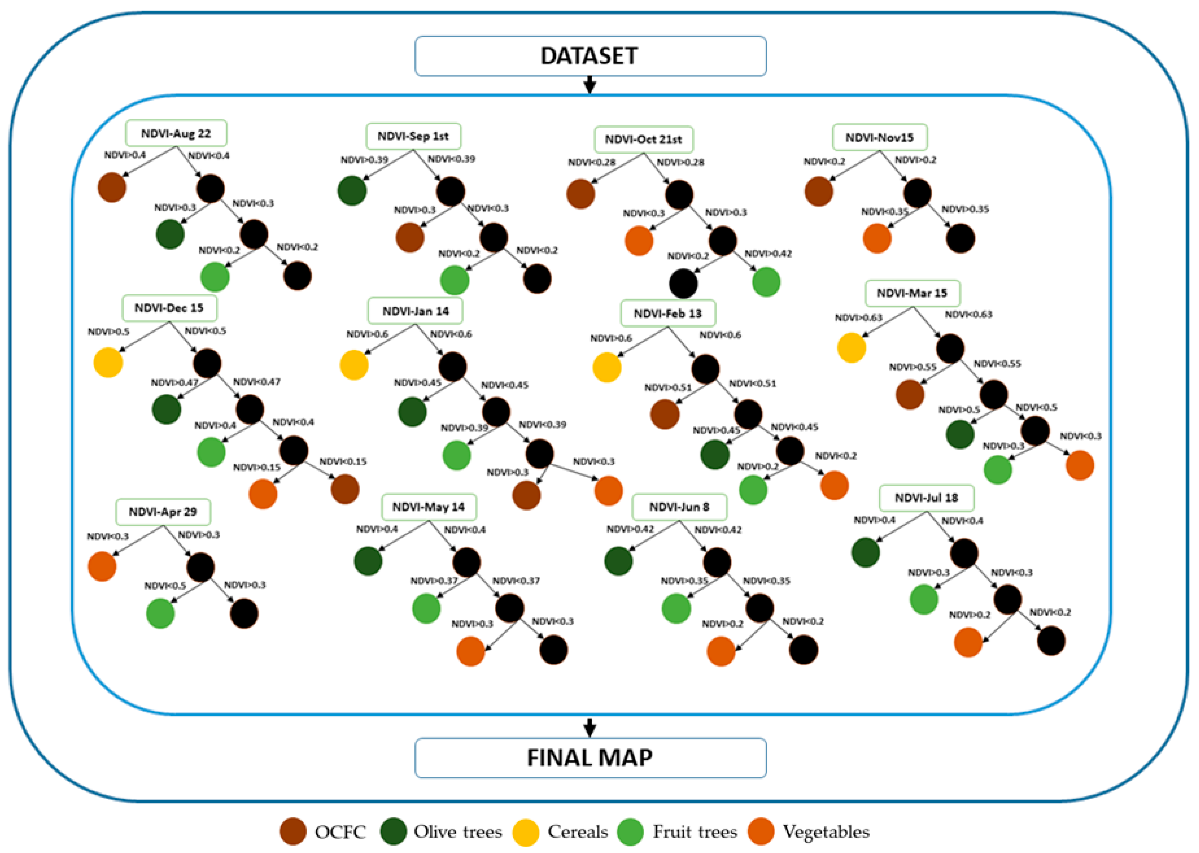
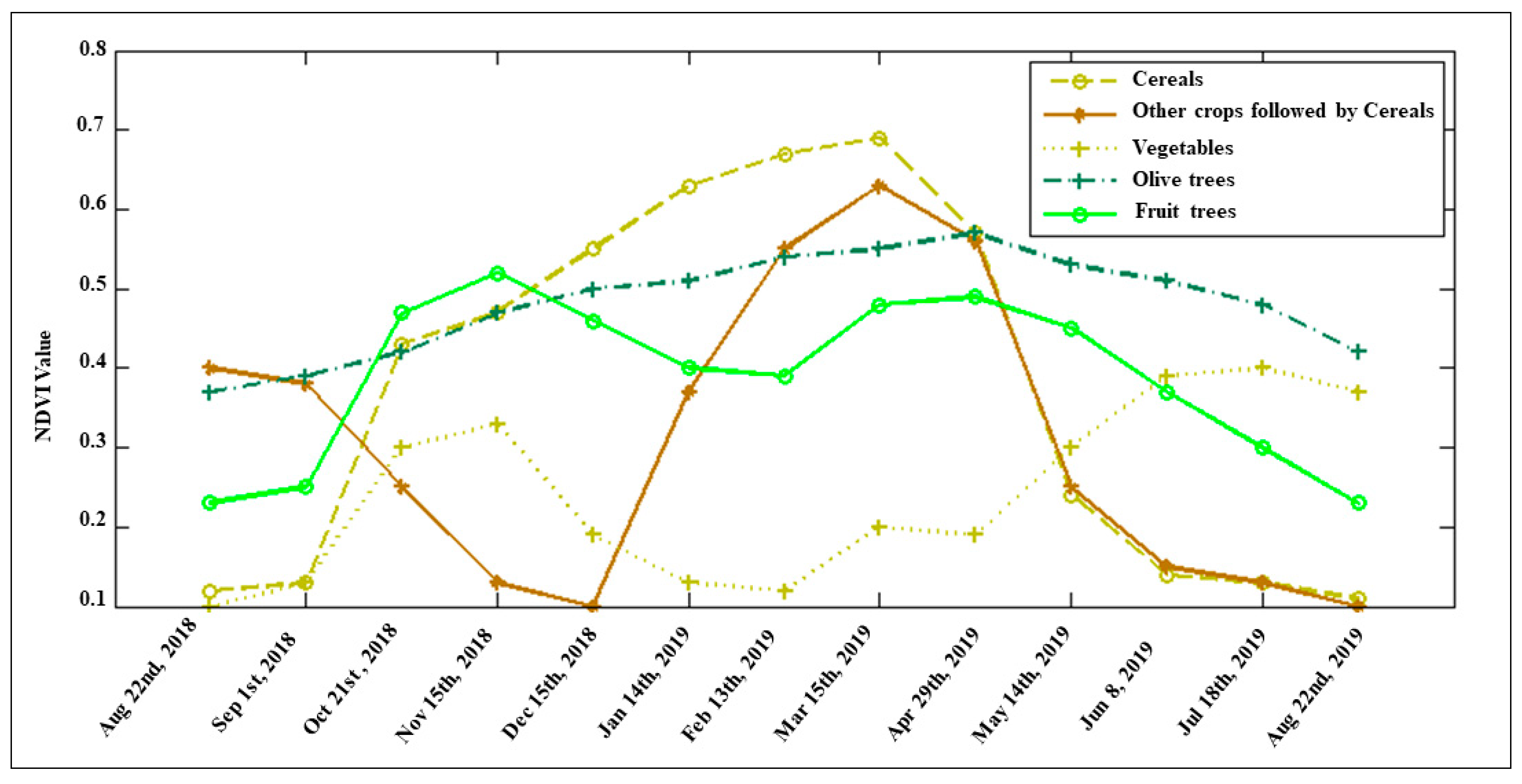
2.6. NDVI Time-Series Spectral Profile Curves
3. Results
3.1. Overall Accuracy
- (i)
- Producer’s accuracy is defined as the probability that a value in a reference dataset was correctly classified. Producer’s accuracy is the complement to the probability of omission error.
- (ii)
- User’s accuracy represents the probability that a resulting value in a certain class is really that class. User’s accuracy is the complement to the probability of commission error.
- (iii)
- Commission errors represent the fraction of the resulting values in a class that does not belong to that class.
- (iv)
- Omission errors represent the fraction of values that belongs to one class but was predicted in a different class.
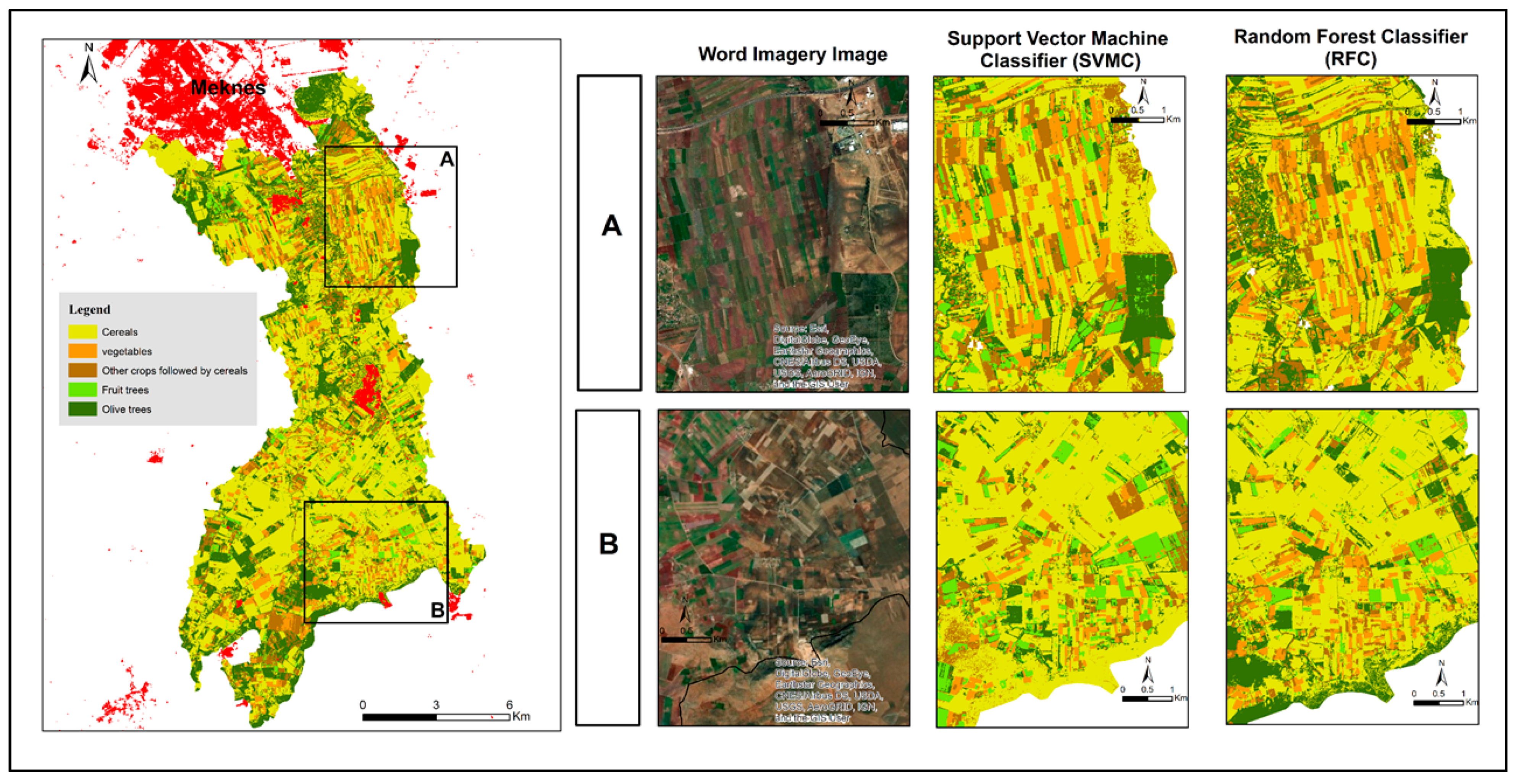
3.2. Crop Mapping
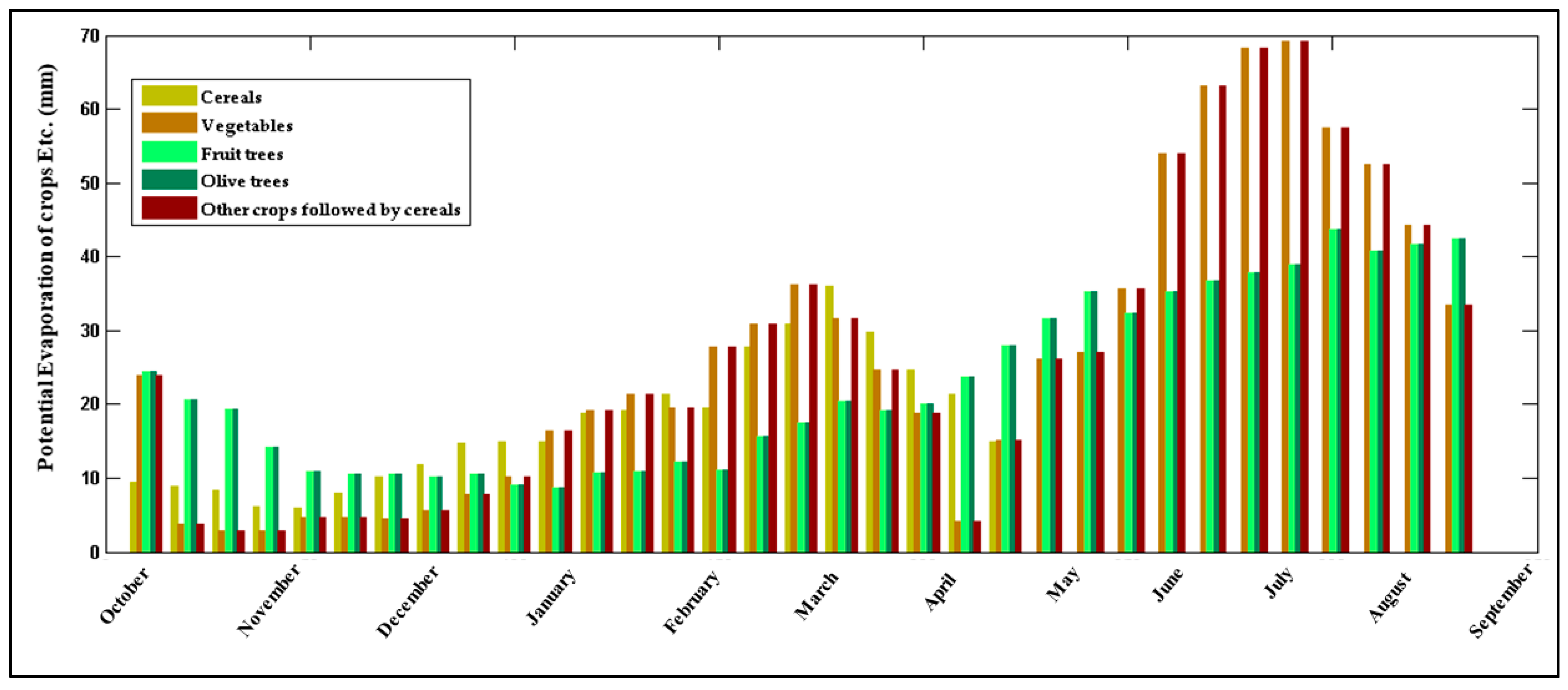
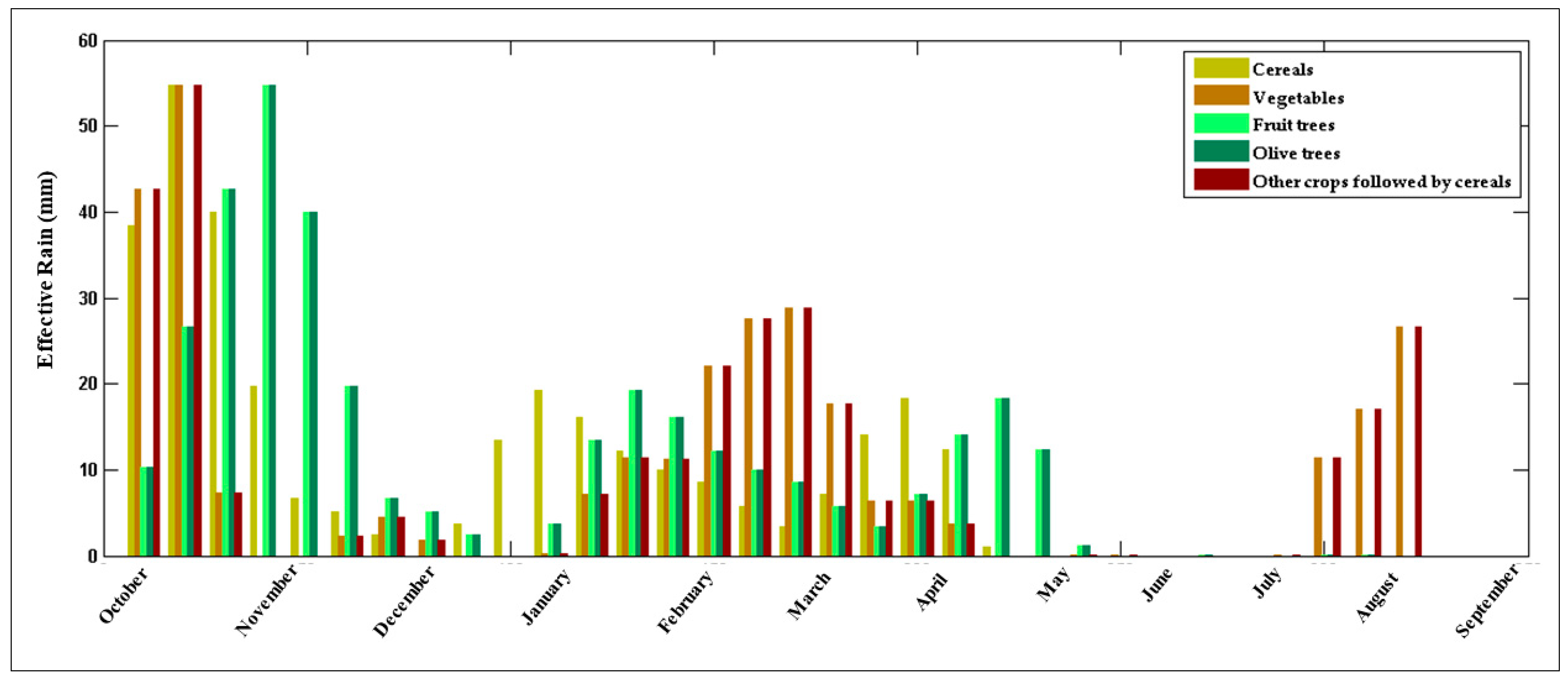
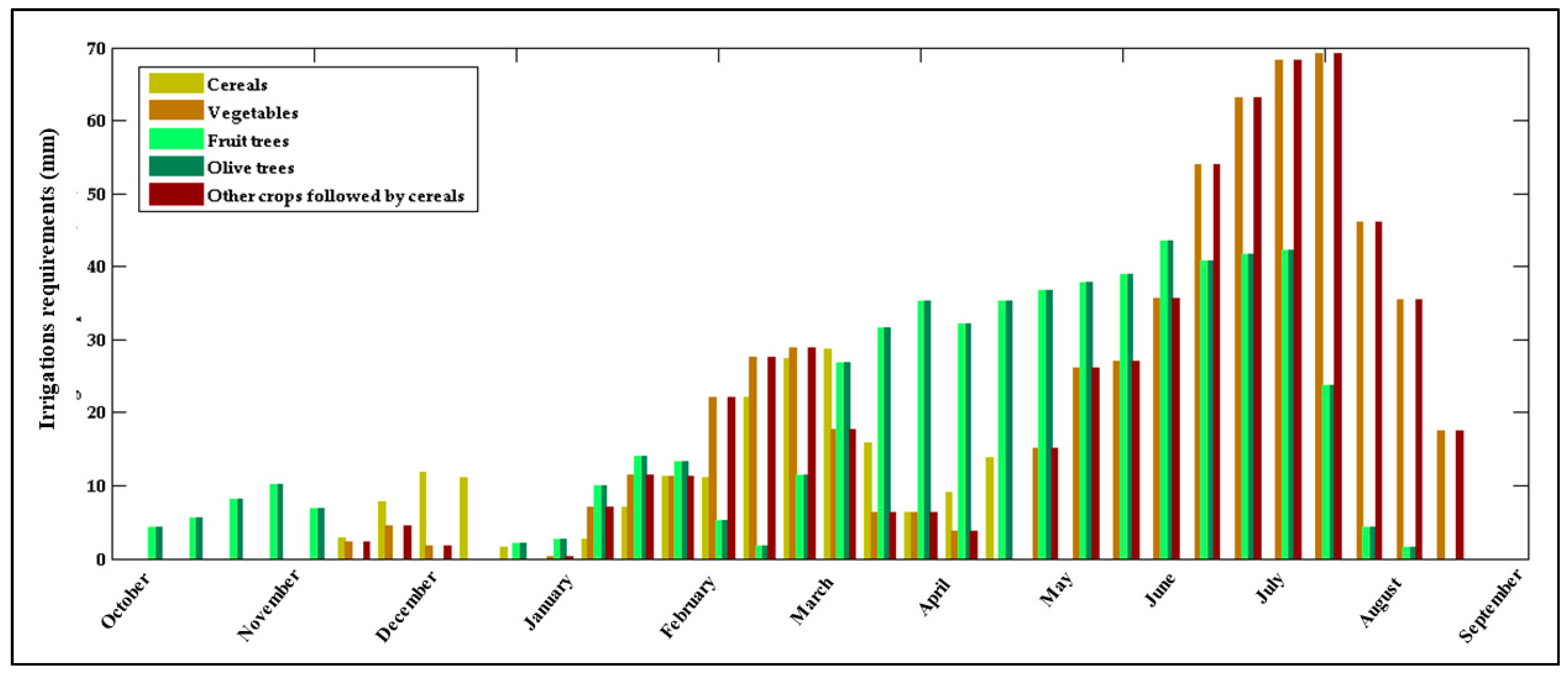
3.3. CROPWAT for Water Crop Requirements
4. Discussion
5. Conclusions
Author Contributions
Funding
Institutional Review Board Statement
Informed Consent Statement
Acknowledgments
Conflicts of Interest
References
- Beckers, V.; Poelmans, L.; Van Rompaey, A.; Dendoncker, N. The Impact of Urbanization on Agricultural Dynamics: A Case Study in Belgium. J. Land Use Sci. 2020, 15, 626–643. [Google Scholar] [CrossRef]
- Mazoyer, M.; Roudart, L. A History of World Agriculture: From the Neolithic Age to the Current Crisis; NYU Press: Manhattan, NY, USA, 2006. [Google Scholar]
- Ouzemou, J.-E.; El Harti, A.; Lhissou, R.; El Moujahid, A.; Bouch, N.; El Ouazzani, R.; Bachaoui, E.M.; El Ghmari, A. Crop Type Mapping from Pansharpened Landsat 8 NDVI Data: A Case of a Highly Fragmented and Intensive Agricultural System. Remote Sens. Appl. Soc. Environ. 2018, 11, 94–103. [Google Scholar] [CrossRef]
- Almazroui, M.; Nazrul Islam, M.; Saeed, S.; Alkhalaf, A.K.; Dambul, R. Assessment of Uncertainties in Projected Temperature and Precipitation over the Arabian Peninsula Using Three Categories of Cmip5 Multimodel Ensembles. Earth Syst. Environ. 2017, 1, 1–20. [Google Scholar] [CrossRef] [Green Version]
- Driouech, F.; Déqué, M.; Sánchez-Gómez, E. Weather Regimes—Moroccan Precipitation Link in a Regional Climate Change Simulation. Glob. Planet. Chang. 2010, 72, 1–10. [Google Scholar] [CrossRef]
- El Hafyani, M.; Essahlaoui, A.; Van Rompaey, A.; Mohajane, M.; El Hmaidi, A.; El Ouali, A.; Moudden, F.; Serrhini, N.-E. Assessing Regional Scale Water Balances through Remote Sensing Techniques: A Case Study of Boufakrane River Watershed, Meknes Region, Morocco. Water 2020, 12, 320. [Google Scholar] [CrossRef] [Green Version]
- El Moçayd, N.; Kang, S.; Eltahir, E.A.B. Climate Change Impacts on the Water Highway Project in Morocco. Hydrol. Earth Syst. Sci. 2020, 24, 1467–1483. [Google Scholar] [CrossRef] [Green Version]
- Lebrini, Y.; Boudhar, A.; Hadria, R.; Lionboui, H.; Elmansouri, L.; Arrach, R.; Ceccato, P.; Benabdelouahab, T. Identifying Agricultural Systems Using SVM Classification Approach Based on Phenological Metrics in a Semi-Arid Region of Morocco. Earth Syst. Environ. 2019, 3, 277–288. [Google Scholar] [CrossRef]
- Barakat, A.; Ouargaf, Z.; Khellouk, R.; El Jazouli, A.; Touhami, F. Land Use/Land Cover Change and Environmental Impact Assessment in Béni-Mellal District (Morocco) Using Remote Sensing and GIS. Earth Syst. Environ. 2019, 3, 113–125. [Google Scholar] [CrossRef]
- Mohajane, M.; Essahlaoui, A.; Oudija, F.; El Hafyani, M.; Hmaidi, A.E.; El Ouali, A.; Randazzo, G.; Teodoro, A.C. Land Use/Land Cover (LULC) Using Landsat Data Series (MSS, TM, ETM+ and OLI) in Azrou Forest, in the Central Middle Atlas of Morocco. Environments 2018, 5, 131. [Google Scholar] [CrossRef] [Green Version]
- Rogan, J.; Chen, D. Remote Sensing Technology for Mapping and Monitoring Land-Cover and Land-Use Change. Prog. Plan. 2004, 61, 301–325. [Google Scholar] [CrossRef]
- Sciortino, M.; De Felice, M.; De Cecco, L.; Borfecchia, F. Remote Sensing for Monitoring and Mapping Land Productivity in Italy: A Rapid Assessment Methodology. CATENA 2020, 188, 104375. [Google Scholar] [CrossRef]
- Wu, Q.; Li, H.; Wang, R.; Paulussen, J.; He, Y.; Wang, M.; Wang, B.; Wang, Z. Monitoring and Predicting Land Use Change in Beijing Using Remote Sensing and GIS. Landsc. Urban Plan. 2006, 78, 322–333. [Google Scholar] [CrossRef]
- Zhang, Y.; Ye, A. Spatial and Temporal Variations in Vegetation Coverage Observed Using AVHRR GIMMS and Terra MODIS Data in the Mainland of China. Int. J. Remote Sens. 2020, 41, 4238–4268. [Google Scholar] [CrossRef]
- Randazzo, G.; Cascio, M.; Fontana, M.; Gregorio, F.; Lanza, S.; Muzirafuti, A. Mapping of Sicilian Pocket Beaches Land Use/Land Cover with Sentinel-2 Imagery: A Case Study of Messina Province. Land 2021, 10, 678. [Google Scholar] [CrossRef]
- Gerard, F.; Petit, S.; Smith, G.; Thomson, A.; Brown, N.; Manchester, S.; Wadsworth, R.; Bugar, G.; Halada, L.; Bezák, P.; et al. Land Cover Change in Europe between 1950 and 2000 Determined Employing Aerial Photography. Prog. Phys. Geogr. 2010, 34, 183–205. [Google Scholar] [CrossRef] [Green Version]
- Tavares, P.A.; Beltrão, N.; Guimarães, U.S.; Teodoro, A.; Gonçalves, P. Urban Ecosystem Services Quantification through Remote Sensing Approach: A Systematic Review. Environments 2019, 6, 51. [Google Scholar] [CrossRef] [Green Version]
- Waldhoff, G.; Lussem, U.; Bareth, G. Multi-Data Approach for Remote Sensing-Based Regional Crop Rotation Mapping: A Case Study for the Rur Catchment, Germany. Int. J. Appl. Earth Obs. Geoinf. 2017, 61, 55–69. [Google Scholar] [CrossRef]
- Wu, M.; Huang, W.; Niu, Z.; Wang, Y.; Wang, C.; Li, W.; Hao, P.; Yu, B. Fine Crop Mapping by Combining High Spectral and High Spatial Resolution Remote Sensing Data in Complex Heterogeneous Areas. Comput. Electron. Agric. 2017, 139, 1–9. [Google Scholar] [CrossRef]
- Yue, J.; Tian, Q. Estimating Fractional Cover of Crop, Crop Residue, and Soil in Cropland Using Broadband Remote Sensing Data and Machine Learning. Int. J. Appl. Earth Obs. Geoinf. 2020, 89, 102089. [Google Scholar] [CrossRef]
- Boualoul, M.; Randazzo, G.; Lanza, S.; Allaoui, A.; Ouardi, H.E.; Habibi, H.; Ouhaddach, H. The use of remote sensing for water protection in the karst environment of the Tabular Middle Atlas/the causse of El Hajeb/Morocco. In Proceedings of the IX Conference of the Italian Society of Remote Sensing, Firenze, Italy, 30 November–1 December 2018; Volume 2000, p. 16. [Google Scholar]
- Muzirafuti, A.; Boualoul, M.; Barreca, G.; Allaoui, A.; Bouikbane, H.; Lanza, S.; Crupi, A.; Randazzo, G. Fusion of Remote Sensing and Applied Geophysics for Sinkholes Identification in Tabular Middle Atlas of Morocco (the Causse of El Hajeb): Impact on the Protection of Water Resource. Resources 2020, 9, 51. [Google Scholar] [CrossRef]
- Ouardi, H.E.; Boualoul, M.; Ouhaddach, H.; Habibi, M.; Muzarafuti, A.; Allaoui, A.; Amine, A. Fault Analysis and Its Relationship with Karst Structures Affecting Lower Jurassic Limestones in the Agourai Plateau (Middle Atlas, Morocco). Geogaceta 2018, 63, 119–122. [Google Scholar]
- Wieland, M.; Martinis, S. Large-Scale Surface Water Change Observed by Sentinel-2 during the 2018 Drought in Germany. Int. J. Remote Sens. 2020, 41, 4742–4756. [Google Scholar] [CrossRef]
- Bachri, I.; Hakdaoui, M.; Raji, M.; Teodoro, A.C.; Benbouziane, A. Machine Learning Algorithms for Automatic Lithological Mapping Using Remote Sensing Data: A Case Study from Souk Arbaa Sahel, Sidi Ifni Inlier, Western Anti-Atlas, Morocco. ISPRS Int. J. Geo-Inf. 2019, 8, 248. [Google Scholar] [CrossRef] [Green Version]
- Du, P.; Tan, K.; Xing, X. Wavelet SVM in Reproducing Kernel Hilbert Space for Hyperspectral Remote Sensing Image Classification. Opt. Commun. 2010, 283, 4978–4984. [Google Scholar] [CrossRef]
- Liu, Y.; Zhang, B.; Wang, L.; Wang, N. A Self-Trained Semisupervised SVM Approach to the Remote Sensing Land Cover Classification. Comput. Geosci. 2013, 59, 98–107. [Google Scholar] [CrossRef]
- Maulik, U.; Chakraborty, D. A Self-Trained Ensemble with Semisupervised SVM: An Application to Pixel Classification of Remote Sensing Imagery. Pattern Recognit. 2011, 44, 615–623. [Google Scholar] [CrossRef]
- Mohajane, M.; Costache, R.; Karimi, F.; Bao Pham, Q.; Essahlaoui, A.; Nguyen, H.; Laneve, G.; Oudija, F. Application of Remote Sensing and Machine Learning Algorithms for Forest Fire Mapping in a Mediterranean Area. Ecol. Indic. 2021, 129, 107869. [Google Scholar] [CrossRef]
- Fathizad, H.; Ali Hakimzadeh Ardakani, M.; Sodaiezadeh, H.; Kerry, R.; Taghizadeh-Mehrjardi, R. Investigation of the Spatial and Temporal Variation of Soil Salinity Using Random Forests in the Central Desert of Iran. Geoderma 2020, 365, 114233. [Google Scholar] [CrossRef]
- Iqbal, F.; Lucieer, A.; Barry, K. Poppy Crop Capsule Volume Estimation Using UAS Remote Sensing and Random Forest Regression. Int. J. Appl. Earth Obs. Geoinf. 2018, 73, 362–373. [Google Scholar] [CrossRef]
- Izquierdo-Verdiguier, E.; Zurita-Milla, R. An Evaluation of Guided Regularized Random Forest for Classification and Regression Tasks in Remote Sensing. Int. J. Appl. Earth Obs. Geoinf. 2020, 88, 102051. [Google Scholar] [CrossRef]
- Bekele, A.A.; Pingale, S.M.; Hatiye, S.D.; Tilahun, A.K. Impact of Climate Change on Surface Water Availability and Crop Water Demand for the Sub-Watershed of Abbay Basin, Ethiopia. Sustain. Water Resour. Manag. 2019, 5, 1859–1875. [Google Scholar] [CrossRef]
- Birhanu, A.; Murlidhar Pingale, S.; Soundharajan, B.; Singh, P. GIS-Based Surface Irrigation Potential Assessment for Ethiopian River Basin. Irrig. Drain. 2019, 68, 607–616. [Google Scholar] [CrossRef]
- Grammatikopoulou, I.; Sylla, M.; Zoumides, C. Economic Evaluation of Green Water in Cereal Crop Production: A Production Function Approach. Water Resour. Econ. 2020, 29, 100148. [Google Scholar] [CrossRef]
- Lee, S.K.; Dang, T.A. Predicting the Water Use-Demand as a Climate Change Adaptation Strategy for Rice Planting Crops in the Long Xuyen Quadrangle Delta. Paddy Water Environ. 2019, 17, 561–570. [Google Scholar] [CrossRef]
- Paymard, P.; Yaghoubi, F.; Nouri, M.; Bannayan, M. Projecting Climate Change Impacts on Rainfed Wheat Yield, Water Demand, and Water Use Efficiency in Northeast Iran. Theor. Appl. Climatol. 2019, 138, 1361–1373. [Google Scholar] [CrossRef]
- Ruan, H.; Yu, J.; Wang, P.; Wang, T. Increased Crop Water Requirements Have Exacerbated Water Stress in the Arid Transboundary Rivers of Central Asia. Sci. Total Environ. 2020, 713, 136585. [Google Scholar] [CrossRef]
- Severo Santos, J.F.; Naval, L.P. Spatial and Temporal Dynamics of Water Footprint for Soybean Production in Areas of Recent Agricultural Expansion of the Brazilian Savannah (Cerrado). J. Clean. Prod. 2020, 251, 119482. [Google Scholar] [CrossRef]
- Surendran, U.; Sushanth, C.M.; Joseph, E.J.; Al-Ansari, N.; Yaseen, Z.M. FAO CROPWAT Model-Based Irrigation Requirements for Coconut to Improve Crop and Water Productivity in Kerala, India. Sustainability 2019, 11, 5132. [Google Scholar] [CrossRef] [Green Version]
- Surendran, U.; Sushanth, C.M.; Mammen, G.; Joseph, E.J. Modelling the Crop Water Requirement Using FAO-CROPWAT and Assessment of Water Resources for Sustainable Water Resource Management: A Case Study in Palakkad District of Humid Tropical Kerala, India. Aquat. Procedia 2015, 4, 1211–1219. [Google Scholar] [CrossRef]
- Moseki, O.; Murray-Hudson, M.; Kashe, K. Crop Water and Irrigation Requirements of Jatropha curcas L. in Semi-Arid Conditions of Botswana: Applying the CROPWAT Model. Agric. Water Manag. 2019, 225, 105754. [Google Scholar] [CrossRef]
- Brouwer, C.; Heibloem, M. Irrigation Water Management: Irrigation Water Needs. Train. Man. 1986, 3. Available online: https://www.fao.org/3/s2022e/s2022e00.htm (accessed on 20 August 2021).
- Vapnik, V. The Support Vector Method of Function Estimation. In Nonlinear Modeling; Springer: Boston, MA, USA, 1998; pp. 55–85. [Google Scholar]
- Bahari, N.I.S.; Ahmad, A.; Aboobaider, B.M. Application of Support Vector Machine for Classification of Multispectral Data. IOP Conf. Ser. Earth Environ. Sci. 2014, 20, 012038. [Google Scholar] [CrossRef]
- Breiman, L. Random Forests. Mach. Learn. 2001, 45, 5–32. [Google Scholar] [CrossRef] [Green Version]
- Costache, R.; Hong, H.; Pham, Q.B. Comparative Assessment of the Flash-Flood Potential within Small Mountain Catchments Using Bivariate Statistics and Their Novel Hybrid Integration with Machine Learning Models. Sci. Total Environ. 2020, 711, 134514. [Google Scholar] [CrossRef]
- Nefeslioglu, H.A.; Sezer, E.; Gokceoglu, C.; Bozkir, A.S.; Duman, T.Y. Assessment of Landslide Susceptibility by Decision Trees in the Metropolitan Area of Istanbul, Turkey. Math. Probl. Eng. 2010, 2010, 1–15. [Google Scholar] [CrossRef] [Green Version]
- Rouse, J.W., Jr. Monitoring the Vernal Advancement and Retrogradation of Natural Vegetation. NASA/GSFCT Type II Report, Greenbelt, MD, USA. 1973. Available online: https://ntrs.nasa.gov/citations/19730020508 (accessed on 22 August 2021).
- Rouse, J.W., Jr. Monitoring the Vernal Advancement and Retrogradation (Greenwave Effect) of Natural Vegetatioa NASA/GSFCT Type III Final Report, Greenbelt, MD, USA. 1974. Available online: https://ntrs.nasa.gov/citations/19740022555 (accessed on 22 August 2021).
- Congalton, R.G. A Review of Assessing the Accuracy of Classifications of Remotely Sensed Data. Remote Sens. Environ. 1991, 37, 35–46. [Google Scholar] [CrossRef]
- Stehman, S.V. Estimating the Kappa Coefficient and Its Variance under Stratified Random Sampling. Photogramm. Eng. Remote Sens. 1996, 62, 401–407. [Google Scholar]
- Olofsson, P.; Foody, G.M.; Stehman, S.V.; Woodcock, C.E. Making Better Use of Accuracy Data in Land Change Studies: Estimating Accuracy and Area and Quantifying Uncertainty Using Stratified Estimation. Remote Sens. Environ. 2013, 129, 122–131. [Google Scholar] [CrossRef]
- Foody, G.M. Explaining the Unsuitability of the Kappa Coefficient in the Assessment and Comparison of the Accuracy of Thematic Maps Obtained by Image Classification. Remote Sens. Environ. 2020, 239, 111630. [Google Scholar] [CrossRef]
- Doorenbos, J.; Pruitt, W.O. Guidelines for Predicting Crop Water Requirements; FAO irrigation and drainage paper; Food and Agriculture Organization of the United Nations: Rome, Italy, 1977; ISBN 978-92-5-100279-7. [Google Scholar]
- ABHS. Etude D’actualisation du Plan Directeurd’Aménagements Intégrés des Ressources en Eau (PDAIRE) du Bassin Hydraulique de Sebou; ABHS: Fez, Morocco, 2011.


| Image | Acquisition Dates |
|---|---|
| 1 | 22 August 2018 |
| 2 | 1 September 2018 |
| 3 | 21 October 2018 |
| 4 | 15 November 2018 |
| 5 | 15 December 2018 |
| 6 | 14 January 2019 |
| 7 | 13 February 2019 |
| 8 | 15 March 2019 |
| 9 | 29 April 2019 |
| 10 | 14 May 2019 |
| 11 | 8 June 2019 |
| 12 | 18 July 2019 |
| 13 | 22 August 2019 |
| Reference Data (%) | ||||||||||||
|---|---|---|---|---|---|---|---|---|---|---|---|---|
| Map Classes | Cereals | OCFC | Vegetables | Olive Trees | Fruit Trees | Total (%) | ||||||
| Classifier | SVM | RF | SVM | RF | SVM | RF | SVM | RF | SVM | RF | SVM | RF |
| Cereals | 88.23 | 87.40 | 6.05 | 24.43 | 2.05 | 1.52 | 1.21 | 5.17 | 0.65 | 6.17 | 64.17 | 64.32 |
| OCFC | 5.27 | 4.48 | 88.10 | 41.86 | 4.80 | 10.76 | 1.66 | 7.39 | 0.48 | 0.62 | 5.54 | 5.81 |
| Vegetables | 3.97 | 3.30 | 1.88 | 10.96 | 92.61 | 84.30 | 0.97 | 0.39 | 0.39 | 0.06 | 14.63 | 13.13 |
| Olive trees | 2.20 | 3.41 | 3.76 | 13.47 | 0.43 | 0.88 | 94.79 | 70.05 | 2.36 | 23.69 | 11.42 | 10.79 |
| Fruit trees | 0.33 | 1.40 | 0.21 | 9.29 | 0.11 | 2.53 | 1.37 | 17.01 | 96.13 | 69.46 | 4.23 | 5.94 |
| 100 | 100 | |||||||||||
| Classes | Commission (%) | Omission (%) | Producer’s Accuracy (%) | User’s Accuracy (%) | ||||
|---|---|---|---|---|---|---|---|---|
| Classifier | SVM | RF | SVM | RF | SVM | RF | SVM | RF |
| Cereals | 0.74 | 1.91 | 11.77 | 12.60 | 88.23 | 87.40 | 99.26 | 98.09 |
| OCFC | 82.93 | 92.26 | 11.90 | 58.14 | 88.10 | 41.86 | 17.07 | 7.74 |
| Vegetables | 20.49 | 19.38 | 7.39 | 15.70 | 92.61 | 84.30 | 79.51 | 80.62 |
| Olive trees | 15.56 | 33.95 | 5.21 | 29.95 | 94.79 | 70.05 | 84.44 | 66.05 |
| Fruit trees | 9.27 | 53.29 | 3.87 | 30.54 | 96.13 | 69.46 | 90.73 | 46.71 |
Publisher’s Note: MDPI stays neutral with regard to jurisdictional claims in published maps and institutional affiliations. |
© 2021 by the authors. Licensee MDPI, Basel, Switzerland. This article is an open access article distributed under the terms and conditions of the Creative Commons Attribution (CC BY) license (https://creativecommons.org/licenses/by/4.0/).
Share and Cite
El Hafyani, M.; Essahlaoui, A.; Fung-Loy, K.; Hubbart, J.A.; Van Rompaey, A. Assessment of Agricultural Water Requirements for Semi-Arid Areas: A Case Study of the Boufakrane River Watershed (Morocco). Appl. Sci. 2021, 11, 10379. https://doi.org/10.3390/app112110379
El Hafyani M, Essahlaoui A, Fung-Loy K, Hubbart JA, Van Rompaey A. Assessment of Agricultural Water Requirements for Semi-Arid Areas: A Case Study of the Boufakrane River Watershed (Morocco). Applied Sciences. 2021; 11(21):10379. https://doi.org/10.3390/app112110379
Chicago/Turabian StyleEl Hafyani, Mohammed, Ali Essahlaoui, Kimberley Fung-Loy, Jason A. Hubbart, and Anton Van Rompaey. 2021. "Assessment of Agricultural Water Requirements for Semi-Arid Areas: A Case Study of the Boufakrane River Watershed (Morocco)" Applied Sciences 11, no. 21: 10379. https://doi.org/10.3390/app112110379
APA StyleEl Hafyani, M., Essahlaoui, A., Fung-Loy, K., Hubbart, J. A., & Van Rompaey, A. (2021). Assessment of Agricultural Water Requirements for Semi-Arid Areas: A Case Study of the Boufakrane River Watershed (Morocco). Applied Sciences, 11(21), 10379. https://doi.org/10.3390/app112110379