The Ensembles of Machine Learning Methods for Survival Predicting after Kidney Transplantation

Abstract

Machine learning is used to develop predictive models to diagnose different diseases, particularly kidney transplant survival prediction. The paper used the collected dataset of patients’ individual parameters to predict the critical risk factors associated with early graft rejection. Our study shows the high pairwise correlation between a massive subset of the parameters listed in the dataset. Hence the proper feature selection is needed to increase the quality of a prediction model. Several methods are used for feature selection, and results are summarized using hard voting. Modeling the onset of critical events for the elements of a particular set is made based on the Kapplan-Meier method. Four novel ensembles of machine learning models are built on selected features for the classification task. Proposed stacking allows obtaining an accuracy, sensitivity, and specifity of more than 0.9. Further research will include the development of a two-stage predictor.

1. Introduction

Organ transplantation is one of the most outstanding achievements of modern medicine. The use of organ transplants today allows the treatment of many patients who until recently could hope, at best, to continue their painful and limited existence.

The urgency of this problem lies in the fact that in Ukraine, legal issues are not yet fully resolved, and there is a lack of donor bodies [1]. Although many organ transplant centers now operate in Ukraine, the needs of Ukrainians for transplants are only about 2% met. The coronavirus pandemic has made adjustments in the number of transplants. In addition to the lack of organs for transplantation, one of the essential problems of Ukrainian transplantology is selecting a donor-recipient pair, which avoids episodes of acute and chronic rejection of the donor organ by the recipient’s immune system [2].

Organ transplantation can significantly improve patients’ quality of life, often offering a single solution for their survival [3]. However, this area does not generate large data sets of patients due to the severity of comorbidities and the complexity of clinical operations, thus preventing the widespread use of mathematical modeling techniques to predict transplant outcomes [4]. For a successful transplant, the recipient and donor should select tissue proteins called human leukocyte antigen (HLA).

The mismatch of HLA between the transplant recipient and their donor can lead to the production of antibodies against HLA, leading to failed transplantation and possibly unsuccessful re-transplantation if it has an HLA-type that is reactive with antibodies [5].

Data-driven approach is used in medicine. Paper [6] presents ensemble of statistical methods usage for kidney transplant survival prediction. Authors in [7] used prediction model to estimate time on a kidney transplant waiting list. The [8] proposes the overview of existing machine learning approaches, particularly, decision tree, artificial neural networks (ANN) with different configuration, Bayesian belief network, logistic regression. The feature selection and several widely-used machine learning models comparison is proposed in [9]. The combination of two predictive models is used for frailty conditions prediction in [10]. That is why the ensemble of machine learning models can be used for early kidney transplant survival prediction.

The main objectives of this study are to use the Kapplan-Meier method and machine learning ensembles to independently confirm the key risk factors associated with early graft rejection (within the first 30 days after transplantation) by changes in the main laboratory parameters of general blood, biochemical analysis of blood and urine conditions of a limited number of immunological laboratory tests.

The paper contribution is forming as the following:

• The own dataset of 164 patients who received HLA-compatible renal allografts between 1992 and 2020 is collected (https://doi.org/10.6084/m9.figshare.14906241.v1, accessed on 4 July 2021);
• Feature selection is built of the ensemble consists of information gain, Boruta and Recursive Feature Elimination. Hard voting is used for obtained results. This allows to choose the significant variables and increase the predictive accuracy on 0.03;
• Decision forest, Logistic regression, AdaBoost, Perceptron, K Nearest neighbor, Random Forest and Support Vector Machine are used as weak classifiers for ensembles construction;
• Four ensembles are built on selected features for the classification task; this allows to obtain the accuracy of more than 0.9;
• Kapplan-Maier method is used for modeling the processes of the onset of critical events for the elements of a particular set.

The remaining of this paper is organized as follows. Section 2 presents the description of the novel ensemble for feature selection. In Section 3, we discuss the proposed approach and compare the results. Finally, Section 4 and Section 5 draw the final conclusions.

2. Materials and Methods

2.1. Dataset Description

Outpatient case histories of 164 patients who received HLA-compatible renal allografts between 1992 and 2020 were retrospectively analyzed: 152 patients underwent transplantation for the first time—64 (42.1%) women and 88 (57.9%) male patients with a mean age of 32.6 ± 8.7 years (range = 18–60 years) at the time of transplantation, and 12 patients (5 (41.7%) women and 7 (58.3%) men), who received a second transplant kidney, who were on an outpatient basis in the Department Hospital Nephrology and Dialysis of the Lviv Regional Clinical Hospital (LRCH).

The study used a group of patients in whom transplantation was performed for the first time. Transplantation in Ukraine (Lviv, Kyiv, Zaporizhia, Kharkiv, Odessa) was performed in 79.6% of patients and other countries (Belarus, Poland, Italy, Turkey, Austria, China, Pakistan) 20.4% of patients. 86.2% of patients from Ukraine received a kidney from a family donor, 13.8% of patients, all from abroad, received a tube kidney. Acute rejection crisis occurred in 13.1% of patients, with cessation of graft function during the perioperative period.

Dataset consists of 80 features and one target attribute (feature characteristics are given in Appendix A). 38 columns consist of more than 60% of missing data. Often, common methods such as mean, median, mode, frequent data, and constant do not provide correct data for missing values. That is why Multiple Imputation by Chained Equations (MICE) [11] was used to impute missing data for these attributes. However, the standard deviation is changed more than 15%. That is why 38 columns were eliminated. Forty-two features were left. The preprocessed dataset is available https://doi.org/10.6084/m9.figshare.14906241.v1, accessed on 4 July 2021.

2.2. Clinical Studies

Studies of HLA genes were performed in the immunological laboratory of Lviv Regional Clinical Hospital following the instructions for using a set of sera of antileukocyte fluids HLA-A, B, C, DR (HLA-serum). Typing of HLA class I and II alleles using lymphocytotoxicity test. The strength of the action is determined on an 8-point scale. In this retrospective analysis, the history of renal dysfunction and other participants were obtained from personal history. The study used a cross-match according to a method that complements complement-dependent cytotoxicity [12,13].

Viral infections were determined by enzyme-linked immunosorbent assay and standard polymerase chain reaction methods.

2.3. Data Preprocessing

To perform statistical analysis of the obtained data, we developed analytical tables in the program Statistica 6.1 and Excel (Microsoft Office 2016), in which the collected primary data were entered. RStudio v.1.1.442 software (Slashdot Media, La Jolla, CA, USA) was used for statistical analysis of the obtained data.

First of all, the normality of the distribution in the obtained sample populations was determined using the Shapiro-Francia criterion. The results were presented as:

• mean values and their standard deviations (M ± SD)—in the case of Gaussian distribution,
• medians, 25th, and 75th percentiles: Me [25%; 75%]—in the case of non-Gaussian distribution,
• shares (%).

When assessing the probability of the difference between the results obtained in the compared groups used:

• odd t—criterion—for two groups with Gaussian distribution;
• Mann Whitney U-test—for two groups with non-Gaussian distribution;
• criterion 2 (xi-square)—when comparing particles.

The difference between the groups was considered significant at p < 0.05.

Next, the feature selection is provided. This procedure is organized as follows:

• Imputation:

  ○

  Missing data imputation using Multiple imputations by chained equations algorithm;

• Feature selection:

  ○

  Correlation;

  ○

  Boruta feature selection;

  ○

  Recursive Feature Elimination;

  ○

  Hard voting of the mentioned algorithms.

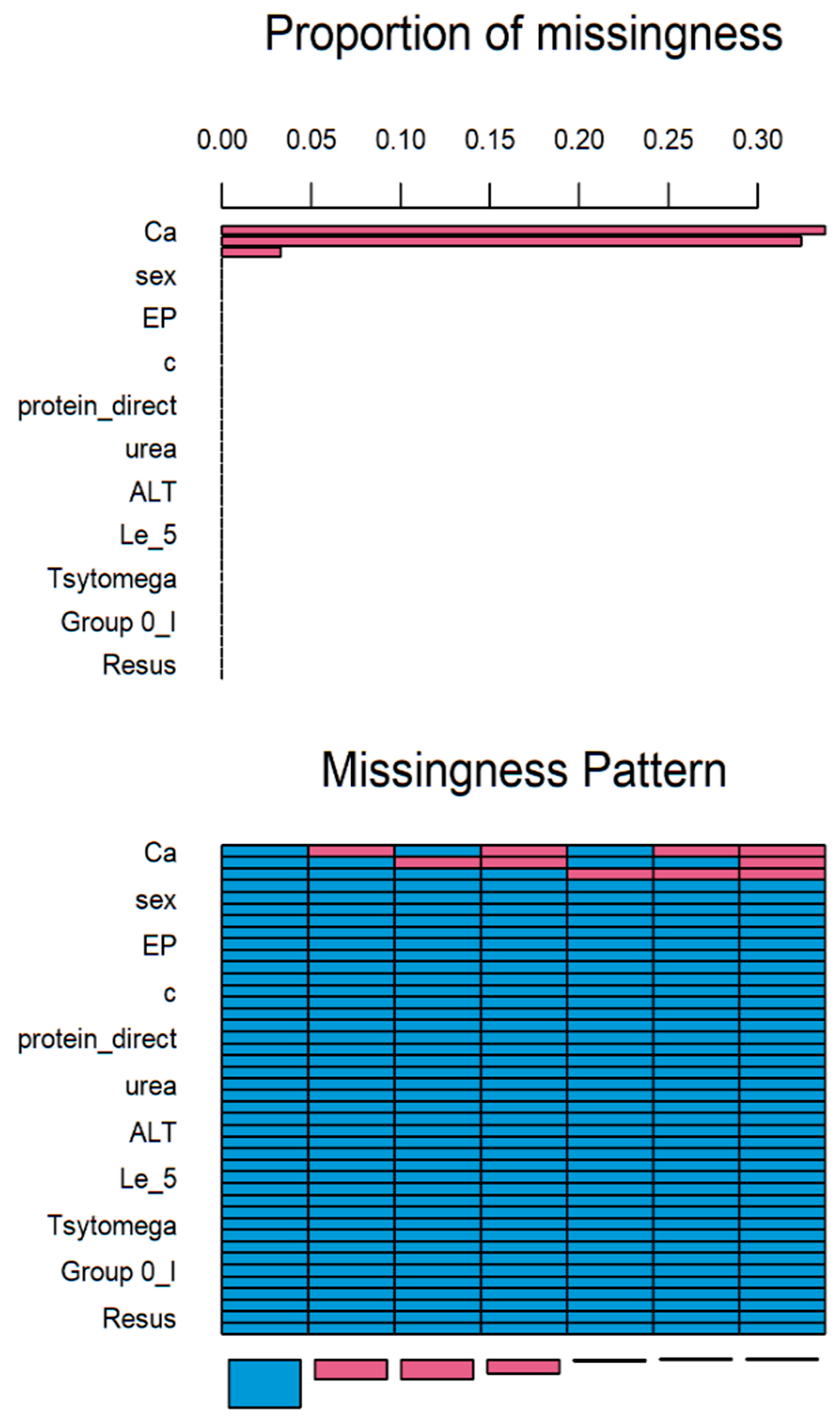
Multiple imputations by chained equations (MICE) is a method for multiple imputations, accounts for the statistical uncertainty in the imputations. In addition, the chained equations approach is very flexible and can handle variables of varying types (e.g., continuous or binary) as well as complexities such as bounds [14]. Based on statistical analysis, more than 30% of values in Ca attribute is missed (Figure 1). Axis x presents the attributes and axis y presents the proportion of missed values. Therefore, this attribute should be eliminated. The rest of the attributes were supplemented.

The imputation summary is given below.

	age	sex	donor_type	duration	HB	EP	Le_norm_4	e	n	c	l	m	ESR
69	1	1	1	1	1	1	1	1	1	1	1	1	1
29	1	1	1	1	1	1	1	1	1	1	1	1	1
28	1	1	1	1	1	1	1	1	1	1	1	1	1
20	1	1	1	1	1	1	1	1	1	1	1	1	1
3	1	1	1	1	1	1	1	1	1	1	1	1	1
1	1	1	1	1	1	1	1	1	1	1	1	1	1
1	1	1	1	1	1	1	1	1	1	1	1	1	1
	0	0	0	0	0	0	0	0	0	0	0	0	0

	protein_direct	protein_total	glucose	creatynin	urea	K	Na
69	1	1	1	1	1	1	1
29	1	1	1	1	1	1	1
28	1	1	1	1	1	1	1
20	1	1	1	1	1	1	1
3	1	1	1	1	1	1	1
1	1	1	1	1	1	1	1
1	1	1	1	1	1	1	1
	0	0	0	0	0	0	0

	ACT	ALT	ZAS_PV	proteint	Epit	Le_5	Er	Tsyl	bacter	Tsytomega
69	1	1	1	1	1	1	1	1	1	1
29	1	1	1	1	1	1	1	1	1	1
28	1	1	1	1	1	1	1	1	1	1
20	1	1	1	1	1	1	1	1	1	1
3	1	1	1	1	1	1	1	1	1	1
1	1	1	1	1	1	1	1	1	1	1
1	1	1	1	1	1	1	1	1	1	1
	0	0	0	0	0	0	0	0	0	0

	hepatitis	hepatitisB	hepatitisC	Group	0_I	Gropu_A_2	Group_B_3
69	1	1	1	1	1	1
29	1	1	1	1	1	1
28	1	1	1	1	1	1
20	1	1	1	1	1	1
3	1	1	1	1	1	1
1	1	1	1	1	1	1
1	1	1	1	1	1	1
	0	0	0	0	0	0

	Group_AB_4			Resus	Class	Hemodializ	Cross-match Ca
69	1	1	1	1	1	1	0
29	1	1	1	1	1	0	1
28	1	1	1	1	0	1	1
20	1	1	1	1	0	0	2
3	1	1	1	0	1	1	1
1	1	1	1	0	1	0	2
1	1	1	1	0	0	0	3
	0	0	0	5	49	51	105

In given above matrix each row corresponds to a missing data pattern (1 = observed, 0 = missing). Rows and columns are sorted in increasing amounts of missing information. The last column and row contain row and column counts, respectively.

Feature selection is built of the ensemble consists of information gain, Boruta and Recursive Feature Elimination. Hard voting is used for obtained results. Only those features which survived the majority of selection algorithms are used.

The correlation more than 0.9 between HB and donor type as well as between EP and HB is founded.

The next, Boruta algorithm was used for features selection. Boruta is a ranking and selection algorithm based on a random forest algorithm [15]. The advantage of Boruta is that it clearly decides whether a variable is important or not, and helps to select statistically significant variables.

Boruta extends the information system by adding copies of all variables and runs a random forest classifier on the extended information system and gather the Z scores computed. This procedure is repeated until the importance is assigned for all the attributes, or the algorithm has reached the previously set limit of the random forest runs. Obviously the larger the feature space and the more variables is redundant to, the larger the number of trees that must be in the forest for a tree where given attribute is not redundant to occur. However, cross-validated is optimal, if forest with a parametrization is used. This effect is why Boruta needs to run dozens of iterations to be effective. One hundred of iterations was provided in our case for depth = 5.

List of most influential variables is given in

Table 1. The selected variables using Boruta algorithm.

Variable	Importance
duration	14.467237
HB	9.093006
EP	7.019778
C	3.429483
L	3.916523
ESR	5.835604
protein_total	8.247771
creatynin	4.757022
Na	3.222748
proteint	5.081887
Epit	4.409411
Er	5.147599
Hemodializ	5.600387

.

The next feature selection using Recursive Feature Elimination [16] is provided.

Recursive Feature Elimination (RFE) is a feature selection approach. It works by recursively removing attributes and building a model based on the attributes that remain. It uses the model’s fidelity to determine which attributes (and combinations of attributes) contribute most to predicting the target attribute.

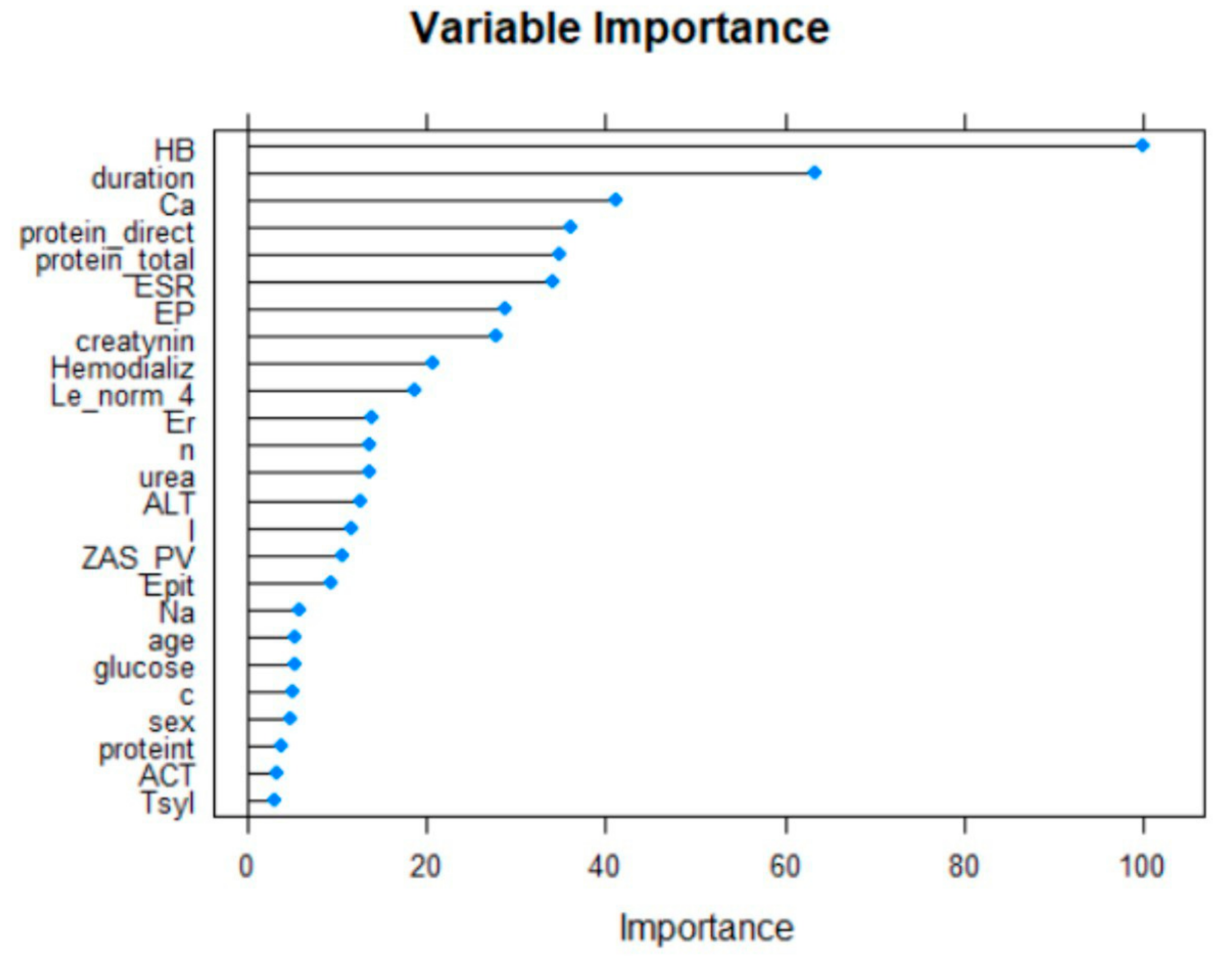
The twenty-five most important variables are shown below (Figure 2).

The next feature selector is built on information gain. The attributes that contribute more information will have a higher information gain value and can be selected (

Table 2. The selected variables using information gain.

Name	Attr_Importance
Duration	0.19901509
HB	0.13819499
EP	0.10945631
C	0.07489602
L	0.07882324
ESR	0.11394131
protein_total	0.12325976
creatynin	0.09308451
protein	0.09190583
Er	0.09911551
Hemodializ	0.07848807

).

Hard voting [17] is the simplest case of a majority vote. In this case, the important features are selected by the majority of the information gain, Boruta and RFE results.

The final dataset consists of 20 selected features given in

Table 3. The results of feature selection.

Variable	Importance
duration	100.000
protein_total	29.297
HB	19.060
ESR	16.346
Hemodializ	14.603
Epit	11.830
protein_direct	11.146
Le_norm_4	11.108
L	9.951
Er	9.742
proteint	9.099
creatynin	9.012
N	8.937
C	8.261
ALT	7.452
EP	7.147
Na	4.814
Urea	4.646
ZAS_PV	3.950
glucose	3.790

.

2.4. The Modeling of the Key Risk Factors Associated with Early Graft Rejection

In the study of cumulative graft survival among patients, the censored Kaplan-Meier method [18] was used. The significance of the difference in the difference in survival levels in individual groups was determined using a logarithmic rank coefficient.

In clinical practice today, the most common survival analysis method for describing censored observations is a Kaplan-Meier method. This method allows you to estimate the proportion of patients who did not have a terminal event and estimate the probability of the absence of an event (to stay alive) by a specific point in time from the beginning of the observation. This probability is called survival, the function of the dependence of survival on time—The function survival rate.

The Kaplan-Meier method is often called the multiplier by the Kaplan-Meier estimate since the value of the survival function at some point in time is the product of the probabilities of survival for all previous points in time. When the analyzed event occurs, the proportion of observed patients is calculated for whom this event has not yet been occurred. In this calculated proportion of patients, there is a probability of surviving the moment of the onset of event i for observed patients. According to the rule of multiplication of probabilities, we obtain the cumulative probability of surviving until the event i occurs for the entire study group of patients [19].

A typical application might involve grouping patients into categories in medical statistics, for instance, those with Gene A profile and those with Gene B profile. In the graph, patients with Gene B die much quicker than those with Gene A. After two years, about 80% of the Gene A patients survive, but less than half of the patients with Gene B.

To generate a Kaplan–Meier estimator, at least two pieces of data are required for each patient (or each subject): the status at last observation (event occurrence or right-censored), and the time to event (or time to censoring). If the survival functions between two or more groups are to be compared, then the third piece of data is required: the group assignment of each subject [20].

2.5. The Modeling of the Key Risk Factors Using Machine Learning Algorithms

The weak classifiers given below are used for classification. After that, the ensembles will be built.

The k Nearest Neighbor (k-NN) method is a metric algorithm for automatically organizing objects. This classifier is used for organ transplantation tasks in [21]. The main principle of the nearest neighbor method is that the object is assigned to the class that is most common among the neighbors of a given element. Mathematically, the classification using k-NN is reduced to the calculation:

$$CS{V}_i\left(d_j\right)={\displaystyle \sum }_{d_z\in T{R}_k\left(d_j\right)}RSV\left(d_j,{\stackrel{}{d}}_z\right)\cdot c{a}_{iZ}$$

(1)

where CSV is categorization status value of object $d_j$, Tr_k(d_j) is the set k of objects ${\stackrel{}{d}}_z$, for which we achieve the maximum of $RSV\left(d_j,{\stackrel{}{d}}_z\right)$, $RSV\left(d_j,{\stackrel{}{d}}_z\right)$—(retrieval status value) similarity measure between training dataset d_j and object ${\stackrel{}{d}}_z$, $c{a}_{iZ}$—Value of the target attribute, k—Threshold (number of objects) indicated how many similar objects we have to be considered to calculate $CS{V}_i\left(d_j\right)$. Any similarity function, either a probabilistic or a vector measure, can be used for these purposes.

Logistic regression is used for classification [22]. Input values (x) are combined linearly, using weights or coefficient values (Beta) to predict the output value (y). The key difference from linear regression is that the initial simulated value is binary (0 or 1), not a numeric value.

The following is an example of a logistic regression equation:

$$y=\frac{e^{\left(b_0+b_1\ast x\right)}}{1+e^{\left(b_0+b_1\ast x\right)}}$$

(2)

where y is the predicted output, b₀ is the offset or interception, b₁ is the coefficient for a single input value (x). In each input data column, there is a related b coefficient (constant real value), which is obtained from the training sample.

The next method of data classification is the method of Support Vector Machine, SVM [23]. The mathematical formulation of the classification problem is as follows: let X be the space of objects (for example, Rⁿ), Y be our classes (for example, Y = {−1,1}). Specified training sample: You need to construct a function F:X→Y (classifier) that maps the class y of the object x.

The classification function F takes the form $F\left(x\right)=sign\left(\left(w,\varphi \left(x\right)\right)+b\right)$. Positive certainty is necessary in order for the corresponding Lagrange function in the optimization problem to be limited from below, i.e., the optimization problem would be correctly defined. The accuracy of the classifier depends, in particular, on the choice of the kernel.

A classifier based on a decision tree is a tree whose inner vertices are denoted by terms, and the edges are marked with test scales [24]. The weight of the term in the vector representation of the test example is compared with these test scales. The leaves of such a tree are marked with category values. The classifier sequentially passes along the vertices of the tree, comparing the weight of the term of the current vertex in the presentation of the test example and determining the further direction of the bypass until it reaches the sheet. The value of the category of a given sheet is assigned to the test example.

The advantage of the decision tree is the ability to visualize the results and interpret the data obtained when obtaining a forecast.

A random forest is a classifier consists of a set of trees $\left\{\mathrm{h}\left(\mathrm{x},{\mathsf{\theta }}_{\mathrm{k}}\right)\mathrm{k}=1,\dots \right\}$, where ${\mathsf{\theta }}_{\mathrm{k}}$ is independent equally distributed random vectors; each tree contributes one vote in determining class X [24]. According to this definition, a random forest is a classifier consisting of an ensemble of decision trees, each of which is built using bagging. In this case, ${\mathsf{\theta }}_{\mathrm{k}}$ is an independent equally distributed l-dimensional random vector, the coordinates of which are independent discrete random variables that take values from the subset {1,2,3,… l} with equal probabilities. The implementation of a random vector ${\mathsf{\theta }}_{\mathrm{k}}$ determines the precedent numbers of the training sample, which form the bootstrap (i.e., the return sample, more details in the following sections) of the sample used in constructing the k-th decision tree.

The averaging of observational results can give a more stable and reliable estimate, as the effect of random fluctuations in a single dimension is weakened. The development of algorithms for combining models was based on a similar idea. The construction of their ensembles turned out to be one of the most powerful machine learning methods, which often surpasses other methods in the quality of forecasts.

One solution that provides the necessary variety of models is their re-learning on samples randomly selected from the general population or other subsets of data constructed from existing ones. To obtain a stable forecast, the predictions of these models are combined in one way or another, for example, by simple averaging or voting (possibly weighted).

Statistical bootstrap (bootstrapping) is a practical computer method for determining statistics of probability distributions based on multiple generations of samples by the Monte Carlo method based on the available sample. Allows you to easily and quickly evaluate various statistics (confidence intervals, variance, correlation, and so on) [25].

Just as the averaging of several observations reduces the estimate of data variance, a reasonable way to reduce the forecast variance is to obtain a large number of data from the general population, build a predictive model for each training sample and average the forecasts obtained. If instead of separate training samples (which we, as a rule, always do not have enough) to execute a bootstrap and based on the generated pseudo-samples to construct n trees of regression, the average collective forecast ${\widehat{f}}_{bag}$ will have a lower variance. This procedure is called bootstrap. Bagging can be performed with respect to regression trees and other models: reference vectors, linear discriminants, Bayesian probabilities, and others.

Another method of improving forecasts is boosting, which is an iterative process of sequential construction of private models [26]. Each new model is learned using the information about the mistakes made in the previous step. The resulting function is a linear combination of the whole ensemble of models while minimizing the penalty function. Like bagging, boosting is a general approach that can be applied to many statistical methods of regression and classification. Here we will limit ourselves to discussing gradient boosting in the context of regression trees.

The AdaBoost is model where for any subsequent model the check and elimination of observations-emissions, erroneous conclusions of the previous model are carried out [27].

Stacking (Stacked Generalization) is a combination of heterogeneous classifiers [26]. To do this, models of any type are combined to create a composite model. It is similar to bagging, but is not limited to the decision tree. The initial data for basic training create features that can recombine with the data. A majority vote or weighing can combine basic training inputs. Additional data for retention is required if meta-learning parameters are used. It also increases the complexity of the model.

3. Results

3.1. Kaplan-Meier Method Results

All objects with a relative kidney transplant had chronic stage V kidney disease. The causes of end-stage renal disease were: chronic glomerulonephritis—99 (65.1%) patients, malformations of the urinary system—23 (15.1%) patients, systemic connective tissue disease—9 (5.9%) patients (systemic lupus erythematosus) —4, systemic scleroderma—1, Sharpe’s disease—1 and rheumatoid arthritis—1, systemic vasculitis—2), type 1 diabetes—9 (5.9%) patients and chronic pyelonephritis—12 (7.9%) patients.

Among 152 patients with primary transplantation: 93 (61.2%) were on chronic hemodialysis, 14 (9.2%) on peritoneal dialysis and 45 (29.6%) without hemodialysis. I (0) blood group was 48 (31.6%) patients, II (A) group—67 (44.1%) patients, III (B)—26 (17.1%), IV (AB)—11 (7.3%). Rhesus factor—positive—137 (90.1%) patients, and negative 15 (9.9%) patients.

In our study, Kaplan-Mayer survival curves in the peroration period (0–30 days) were as follows. In the group of patients (38.8%) after transplantation without hemodialysis before transplantation, the survival results were significantly better (p = 0.001) than in the group of patients (61.2%) with previous hemodialysis (Figure 3). No significant difference was found between age and sex (p < 0.05).

According to the indicators of the general blood analysis, a probable difference (p = 0.049) was found between the groups of patients with normal leukocytes in the blood (59.2%) and the group with leukocytosis in the blood (38.8%), due to better survival results in the first group (Figure 4), on other indicators of the general analysis of blood the probable difference (p < 0.05) was not established.

The biochemical analysis of blood revealed a probable fundamental difference in the levels of creatinine (p = 0.00001) and urea (p = 0.01), between normal values and elevated levels. Creatinine levels were higher than normal in 26.9% of patients, compared with 72.1% (Figure 5), and urea levels were higher than normal in 56.7% of patients, compared with 43.3% of patients with urea was normal (Figure 6), among other indicators of biochemical analysis of blood, no significant difference was found (p < 0.05).

From the indicators of the general analysis of urine, the indicators of proteinuria were probable (p = 0.0005): the percentage of patients with increased proteinuria was 64.5% of patients, compared with 35.5% of patients with normal protein levels (Figure 7). The level of erythrocytes in the urine was probably (p = 0.00001) higher in 34.8% of patients, compared with 65.2% of patients with erythrocytes within normal limits (Figure 8). No significant difference was found between other indicators of the general analysis of urine (p < 0.05).

No significant difference in transplant survival was found between the immunological indicators of the cross-match test 0–10% and the indicators of 10–20%. HLA-typing between matches 0–3 and 4–6 matches also did not show a significant difference in transplant survival.

3.2. ML Models and Developed Ensembles Results

The research methodology is organized as follows:

• We divide the available sample into training and testing. For training, we will select 70% of the original sample.
• We train nine models for selected features, for selected and tentative features, and the whole dataset, respectively:
  • Decision forest (RTree using CART algorithm, tuning parameters is used too),
  • Logistic regression (LG, without L1 or L2 regularization),
  • Built-in Adaptive Boosting (AdaBoost),
  • Perceptron (MLP, hyperparameters after Bayesian Optimization {‘activation’: ‘sigmoid’, ‘batch_size’: 209, ‘epochs’: 87, ‘layers1’: 15, ‘layers2’: 3, ‘learning_rate’: 0.07160}),
  • K Nearest neighbor (We will estimate three hyperparamters, namely n-neighbors, weights and metric. Next, the Exhaustive Grid Search technique for hyperparameter optimization is used. Since we have provided the class validation score as 3 (cv = 3), Grid Search will evaluate the model 6 × 2 × 3 × 3 = 108 times with different hyperparameters. The best values are the following: n_neighbors = 5, weights = ‘uniform’, algorithm = ‘brute’, metric = ‘minkowski’),
  • Random Forest (RF, 500 trees and the maximum depth is equal to 8),
  • Support vector Machine with Polynomial (SVMPoly, Grid Search is used too, hyperparameters C = 10, gamma=0.0001),
  • Support vector Machine with Radial (SVMRadial, Grid Search is used too, hyperparameters C = 10, gamma=0.0001),
  • Support vector Machine with Linear (SVMLin, Grid Search is used too, hyperparameters C = 10, gamma=0.0001).
• We built four ensembles:
  • Boosted random forest,
  • Boosted logistic regression,
  • Bagged decision tree based on CARD algorithm,
  • Stacking.
• We carry out resampling of the obtained models, perform a statistical analysis of two generated model quality metrics (Accuracy and J. Cohen’s Kappa index) on the training set, rank the models, and estimate the confidence intervals of the criteria used.
• The analysis is organized for the whole dataset and selected features, respectively. That is why the research methodology is used separately for the whole dataset and dataset based on selected features.
• We check is the model overfitted using k-fold.

At the first stage, the separated machine learning models are analyzed. The worst accuracy is for MLP trained on the whole dataset and selected features (Table 3). The best weak classifier is ADABOOST, with an accuracy equal to 0.8533677. That is why MLP classifier is excluded.

The difference in accuracy for the whole dataset and selected features for each model is given in Table 3 in the last column. The accuracy of LG is low for the entire dataset but 0.13848 higher for the selected features.

At the next stage, two Boosting modes based on regression tree and logistic regression are built. Bosted LG shows higher accuracy than all weak classifiers built on the whole dataset. However, the result of SVMRadial built on selected features is better than for boosted ensembles.

Bagged CART without tuned parameters is trained at the next stage. However, the accuracy of this ensemble is worse than for boosted LG both for all features and for selected features.

The next step is the combination of multiple predictors using stacking. KNN, SVMLin, SVMPoly, SVMRadial, rtree, logistic regression (LG) are used for ensemble development. The random forest (RF) algorithm combines the predictions. 100 trees are built for RF. Tuning parameters are used too.

Ensemble results are given below for the whole dataset.

Accuracy and Kappa index are used for results evaluation.

Random Forest results:

• 207 samples,
• 6 predictors,
• 2 classes: ‘first_class’, ‘second_class’
• No pre-processing
• Resampling: Cross-Validated (10 fold, repeated 3 times)
• Summary of sample sizes: 6, 7, 6, 6, 5, 5, …
• Resampling results across tuning parameters:

mtry	Accuracy	Kappa
2	0.8990257	0.4704559
4	0.8114255	0.4695021

Accuracy was used to select the optimal model using the largest value. The final value used for the model was mtry = 2. Here mtry is the number of variables available for splitting at each tree node.

The

Table 4. Models’ comparison (accuracy).

Model	Results for the Whole Dataset	Results for Selected Features	The Difference in Accuracy
RTree	0.8005724	0.8066330	0.00606
ADABOOST	0.8533677	0.8519529	−0.0014
LG	0.7208754	0.8593603	0.13848
MLP	0.6637374	0.6637374	0
SVMLin	0.7684848	0.8526936	0.08421
SVMPoly	0.8255219	0.8701010	0.04458
SVMRadial	0.7716162	0.8838721	0.11226
KNN	0.8117845	0.8426263	0.03084
RF	0.8467677	0.8489899	0.00222
Bosted rf	0.8373016	0.8489899	0.01169
bosteed glm	0.8656746	0.8501010	−0.0156
bagget CART	0.8380952	0.8489899	0.01089
Stacking	0.8990257	0.9190155	0.01999

summarizes the results of models’comparison. The numbers in the bold present the highest accuracy in the column for weak predictors, boosting models and stacking respectively. The numbers in the italic present the results of developed ensembles of machine learning models. The difference in accuracy column given the difference between model accuracy built on whole dataset and model accuracy built on selected features.

The models comparison is given in Figure 9. The accuracy, specificity and sensitivity are taken into account. Therefore, the proposed ensembles show the good predictive accuracy for both classes too.

The pairwise correlation coefficients for the mentioned sub-models are given in

Table 5. The pairwise correlation coefficients for the sub-models in the stacking ensemble.

Model	rf	LG	knn	svmRadial	svmPoly	svmLinear
Rf	1.0000000	0.6760573	0.5989963	0.4414152	0.6175437	0.4998480
LG	0.6760573	1.0000000	0.4461349	0.1802775	0.4216896	0.5421103
knn	0.5989963	0.4461349	1.0000000	0.5829106	0.5121148	0.2561106
svmRadial	0.4414152	0.1802775	0.5829106	1.0000000	0.6812341	0.3496763
svmPoly	0.6175437	0.4216896	0.5121148	0.6812341	1.0000000	0.4901687
svmLinear	0.4998480	0.5421103	0.2561106	0.3496763	0.4901687	1.0000000

. The pairwise correlation is calculated for ensemble quality estimation. From this table, we can see a generally low correlation for all pairs of predictions. The two methods with the highest correlation between their predictions are Logistic Regression and kNN, with a correlation coefficient of 0.517, which is not considered high (>0.75).

4. Discussion

Given the data obtained, it can be argued that six indicators affect the survival of kidney transplantation in the perioperative period, primarily the lack of previous hemodialysis, high leukocytosis, urea and creatinine in the blood, proteinuria, and erythrocyturia in the urine. Thus, based on these data, the first signs of possible rejection can be predicted based on five general screening laboratory tests.

The data preprocessing allows us to increase the quality of analysis. Boruta, RFE, and information gain are used for feature selection. The results of the selection are formed based on hard voting of all features selectors.

A stacking classifier for early graft rejection prediction algorithm based on combination of 6 weak classifiers was developed in this paper. Random forest algorithm is used to combine the predictions. Using this ensemble allows us to increase the defect prediction accuracy up to 92%. Therefore, the proposed algorithm shows higher accuracy comparing to weak classifiers and boosted and bagged ensembles.

5. Conclusions

This paper presents feature selection and kidney transplant survival for a month after transplantation prediction using Kapplan-Meier method and ensemble classifier. The set of individual parameters from the own dataset was used to predict the key risk factors associated with early graft rejection (within the first 30 days after transplantation) by changes in the main laboratory parameters of general blood, biochemical analysis of blood and urine. Our study shows a high pairwise correlation between a huge subset of the parameters listed in the dataset. Hence the proper feature selection is needed to increase the quality of a prediction model.

Further research will include the development of a two-stage classifier. The first step will be a division of instances by clusters, and the second is analysis of each particular cluster.

References

1. Anikina, G. Features of Legal Regulation of Organ Transplantation from a Dead Organ; Legal Ukraine: Kyiv, Ukraine, 2010; Volume 10, pp. 68–75. [Google Scholar]
2. Chopyak, V.; Potemkina, G.; Gavrilyuk, A.; Kril, I. Clinical Immunology and Allergology: A Textbook; All-Ukrainian Specialized Publishing House “Medicine”: Kyiv, Ukrainian, 2017; p. 224. [Google Scholar]
3. Purnell, T.S.; Auguste, P.; Crews, D.C.; Lamprea-Montealegre, J.; Olufade, T.; Greer, R.; Ephraim, P.; Sheu, J.; Kostecki, D.; Powe, N.R.; et al. Comparison of Life Participation Activities Among Adults Treated by Hemodialysis, Peritoneal Dialysis, and Kidney Transplantation: A Systematic Review. Am. J. Kidney Dis. 2013, 62, 953–973. [Google Scholar] [CrossRef] [Green Version]
4. Díez-Sanmartín, C.; Sarasa Cabezuelo, A. Application of artificial intelligence techniques to predict survival in kidney transplantation: A review. J. Clin. Med. 2020, 9, 572. [Google Scholar] [CrossRef] [Green Version]
5. Higgins, R.; Hathaway, M.; Lowe, D.; Lam, F.; Kashi, H.; Tan, L.C.; Imray, C.; Fletcher, S.; Zehnder, D.; Chen, K.; et al. Blood Levels of Donor-Specific Human Leukocyte Antigen Antibodies After Renal Transplantation: Resolution of Rejection in the Presence of Circulating Donor-Specific Antibody. Transplantation 2007, 84, 876–884. [Google Scholar] [CrossRef]
6. Mark, E.; Goldsman, D.; Gurbaxani, B.; Keskinocak, P.; Sokol, J. Using machine learning and an ensemble of methods to predict kidney transplant survival. PLoS ONE 2019, 14, e0209068. [Google Scholar] [CrossRef] [PubMed] [Green Version]
7. Sapiertein Silva, J.F.; Ferreira, G.F.; Perosa, M.; Nga, H.S.; de Andrade, L.G.M. A machine learning prediction model for waiting time to kidney transplant. PLoS ONE 2021, 16, e0252069. [Google Scholar] [CrossRef] [PubMed]
8. Sekercioglu, N.; Fu, R.; Kim, S.J.; Mitsakakis, N. Machine learning for predicting long-term kidney allograft survival: A scoping review. Ir. J. Med. Sci. 2021, 190, 807–817. [Google Scholar] [CrossRef] [PubMed]
9. Jeong, Y.-S.; Kim, J.; Kim, D.; Woo, J.; Kim, M.; Choi, H.; Kang, A.; Park, S. Prediction of Postoperative Complications for Patients of End Stage Renal Disease. Sensors 2021, 21, 544. [Google Scholar] [CrossRef] [PubMed]
10. Bertini, F.; Bergami, G.; Montesi, D.; Veronese, G.; Marchesini, G.; Pandolfi, P. Predicting Frailty Condition in Elderly Using Multidimensional Socioclinical Databases. Proc. IEEE 2018, 106, 723–737. [Google Scholar] [CrossRef]
11. Mera-Gaona, M.; Neumann, U.; Vargas-Canas, R.; López, D.M. Evaluating the impact of multivariate imputation by MICE in feature selection. PLoS ONE 2021, 16, e0254720. [Google Scholar] [CrossRef]
12. Mulley, W.L.; Canellis, G.N. Under standing crossmatch testing in organ transplantation: A case-based guide for the general nephrologist. Nephrology 2011, 16, 125–133. [Google Scholar] [CrossRef]
13. Bubnova, L.N.; Berkos, A.S.; Nikolenko, V.N. Instructions for use of a set of sera antileukocyte HLA-A, B, C, DR histotyping liquid (HLA serum). Mir. Moscow 1981, 267. [Google Scholar]
14. Kunkel, D.; Kaizar, E.E. A comparison of existing methods for multiple imputation in individual participant data meta-analysis. Stat. Med. 2017, 36, 3507–3532. [Google Scholar] [CrossRef] [PubMed]
15. Anand, N.; Sehgal, R.; Anand, S.; Kaushik, A. Feature selection on educational data using Boruta algorithm. Int. J. Comput. Intell. Stud. 2021, 10, 27–35. [Google Scholar] [CrossRef]
16. Darst, B.F.; Malecki, K.C.; Engelman, C.D. Using recursive feature elimination in random forest to account for correlated variables in high dimensional data. BMC Genet. 2018, 19, 65. [Google Scholar] [CrossRef] [PubMed] [Green Version]
17. Atallah, R.; Al-Mousa, A. Heart Disease Detection Using Machine Learning Majority Voting Ensemble Method. In Proceedings of the 2019 2nd International Conference on New Trends in Computing Sciences (ICTCS), Amman, Jordan, 9–11 October 2019; IEEE: Piscataway, NJ, USA, 2019; pp. 1–6. [Google Scholar]
18. Kurilshikov, A.; Medina-Gomez, C.; Bacigalupe, R.; Radjabzadeh, D.; Wang, J.; Demirkan, A.; Le Roy, C.I.; Garay, J.A.R.; Finnicum, C.T.; Liu, X.; et al. Large-scale association analyses identify host factors influencing human gut microbiome composition. Nat. Genet. 2021, 53, 156–165. [Google Scholar] [CrossRef] [PubMed]
19. Slinin, A.S.; Bydanov, O.I.; Karachunskiy, A.I. Analysis of survival and possibility of certain events in patients with acute leucosis. Pediatric Haematol./Oncol. Immunopathol. 2016, 15, 34–39. [Google Scholar] [CrossRef]
20. Rich, J.T.; Neely, J.G.; Paniello, R.C.; Voelker, C.C.J.; Nussenbaum, B.; Wang, E. A practical guide to understanding Kaplan-Meier curves. Otolaryngol. Neck Surg. 2010, 143, 331–336. [Google Scholar] [CrossRef] [Green Version]
21. Atallah, D.M.; Badawy, M.; El-Sayed, A. Intelligent feature selection with modified K-nearest neighbor for kidney transplantation prediction. SN Appl. Sci. 2019, 1, 1297. [Google Scholar] [CrossRef] [Green Version]
22. Nematollahi, M.; Akbari, R.; Nikeghbalian, S.; Salehnasab, C. Classification Models to Predict Survival of Kidney Transplant Recipients Using Two Intelligent Techniques of Data Mining and Logistic Regression. Int. J. Organ. Transplant. Med. 2017, 8, 119–122. [Google Scholar]
23. Ravikumar, A.; Saritha, R.; Chandra, V. Support vector machine based prognostic analysis of renal transplantations. In Proceedings of the 2013 Fourth International Conference on Computing, Communications and Networking Technologies (ICCCNT), Tiruchengode, India, 4–6 July 2013; IEEE: Piscataway, NJ, USA, 2013; pp. 1–6. [Google Scholar]
24. Shaikhina, T.; Lowe, D.; Daga, S.; Briggs, D.; Higgins, R.; Khovanova, N. Decision tree and random forest models for outcome prediction in antibody incompatible kidney transplantation. Biomed. Signal Process. Control. 2019, 52, 456–462. [Google Scholar] [CrossRef]
25. Hoang, D.T.; Chernomor, O.; Von Haeseler, A.; Minh, B.Q.; Vinh, L.S. UFBoot2: Improving the Ultrafast Bootstrap Approximation. Mol. Biol. Evol. 2018, 35, 518–522. [Google Scholar] [CrossRef] [PubMed]
26. Ribeiro, M.H.D.M.; Coelho, L.D.S. Ensemble approach based on bagging, boosting and stacking for short-term prediction in agribusiness time series. Appl. Soft Comput. 2020, 86, 105837. [Google Scholar] [CrossRef]
27. Javed, A.R.; Jalil, Z.; Moqurrab, S.A.; Abbas, S.; Liu, X. Ensemble Adaboost classifier for accurate and fast detection of botnet attacks in connected vehicles. Trans. Emerg. Telecommun. Technol. 2020, 4, 4088. [Google Scholar] [CrossRef]
Figure 1. Results of MICE imputation.
Applsci 11 10380 g001
Figure 2. The selected variables using RFE algorithm.
Applsci 11 10380 g002
Figure 3. Evaluation of graft function depending on the presence of hemodialysis.
Applsci 11 10380 g003
Figure 4. Evaluation of graft function depending on leukocytosis in the blood.
Applsci 11 10380 g004
Figure 5. Evaluation of graft function depending on creatinine in the blood.
Applsci 11 10380 g005
Figure 6. Evaluation of graft function depending on urea in the blood.
Applsci 11 10380 g006
Figure 7. Evaluation of graft function depending on proteinuria.
Applsci 11 10380 g007
Figure 8. Evaluation of graft function depending on erythrocyturia.
Applsci 11 10380 g008
Figure 9. Models comparison.
Applsci 11 10380 g009aApplsci 11 10380 g009b