Abstract
This paper proposes an online uniform foot location planning method (UPMPC) based on model predictive control (MPC) for solving the problem of large posture changes during gait transitioning. This method converts the foot location planning into a discrete-time MPC problem. The core part of the method is to complete the planning of the foot location based on the linear inverted pendulum (LIP) model and the simplified robot dynamics model. By unifying the input foot location at each time step, the solution time is shortened. The final simulation experiment compares the results of using the UPMPC and foot location planning method with heuristic function (HF) for gait transitioning, respectively. This result demonstrates that the UPMPC can complete the gait transitioning task and adapt to large changes in posture during gait transitioning. In addition, the results also show the good performance of UPMPC in fixed gait.
1. Conventions
To illustrate the content of this paper, the following abbreviations listed in Table 1 are used.

Table 1.
The abbreviations are used in this manuscript.
To illustrate the formulas in subsequent sections, the mathematical notation listed in Table 2 is used. Matrices and vectors are upright and bold. Scalars are italicized.
Table 2.
Main Symbol Conventions in this paper.
2. Introduction
Legged robots have greater environmental adaptability than wheeled and tracked robots. In order to meet the needs of different tasks in various environments, users are no longer satisfied with quadruped robots moving in a fixed gait and expect legged robots to be able to switch stably between multiple gaits during moving.
Quadruped robots usually perform gait transitioning to reduce energy consumption. Horses [1] have varying energy expenditure at different gaits and speeds. In order to maximize energy efficiency, the horse will choose the gait with the least energy consumption at each speed. Quadruped robots designed with reference to quadrupeds naturally have variable energy consumption at different gaits. The energy consumption of a quadruped robot at various gaits and speeds is explored in detail in [2]. Each gait has a significant energy gap at the same speed. It is also found that the long-period, large duty cycle gait and the short-period, low duty cycle gait consume less energy at low and high speeds, respectively. Therefore, it is of utmost importance to switch from a high-energy-consuming gait to a gait with relatively low energy consumption.
However, in actual use, the appropriate gait is also selected according to the task needs. When traversing uneven terrain, it is expected that the impact on the ground is small and the height of the quadruped robot is basically constant while maintaining a certain speed. Thus, the gait chosen at this point may not be the less energy intensive one. The choice of gait is the result of many factors. Therefore, the quadruped robot needs to successfully switch between different gaits at a certain speed, not just from a high-energy-consuming gait to a low-energy-consuming gait.
The successful locomotion of the robot cannot be separated from the choice of the foot location. A lot of researches have been done on foot location planning. HF [3] is a commonly used method. By adjusting the gain parameters, better results can be obtained. The method has been applied in several MIT’s robots [4,5]. Combining HF and MPC [4], MIT’s Mini Cheetah implements multiple gaits. However, the fixed-parameter HF is difficult to cope with transitioning between various gaits with different periods. The properties of gaits are distinct, in the case of different periods, leading to the inability of the fixed-parameter HF to adapt to the large changes of posture after the gait transitioning. The capture point technique which is frequently used in bipedal robots is also a common method for foot location planning. Pratt et al. simplify the bipedal robot into a LIP model with a flywheel, and determine the range of foot locations and the foot location point of the bipedal robot by establishing the capture domain and the capture point where the robot can stop in one step [6]. Simões et al. find the capture domain that can two-step stop based on the capture points and N-Step Capturability theories, and successfully verify the effect of the algorithm on simulation [7]. Seyde et al. [8] and Kojio et al. [9] both utilize capture point theory for foot location planning and achieve good results on bipedal robots. However, the capture point method requires setting the number of steps to stop, which limits the performance of the robot. MPC is capable of generating behavior with a wide range of adaptations based on real-world situations [10]. Saraf et al. use the MPC to complete a terrain adaptive gait transitioning between bounding and trotting [11]. MPC-based foot location planning has also been widely studied. A number of researchers achieve better robustness and interference resistance on quadruped robots based on the LIP model for foot location planning using MPC [12,13,14]. Xin et al. design LIP-based foot location planning using MPC [15]. The method applies the LIP model to predict the COM position and velocity. Furthermore, the prediction result is used as the initial state of MPC for planning the foot location. It is successfully applied not only to quadruped robots but also to bipedal robots, and has good anti-interference capability. However, the calculating time grows rapidly with increasing prediction length.
This paper aims at addressing the transitioning of walking, trotting and flight trotting with different gait periods at the same speed. Walking (four beat or two beat) has a duty cycle greater than 50%. The duty cycle is the proportion of the support period to the entire gait period. Furthermore, the four-legged support period can exist in this gait. The two diagonally opposite legs move together for trotting. The duty cycle of trotting is equal to 50%. The two diagonal opposite leg of the flight trotting gait also moves simultaneously, but differs from trotting in that the duty cycle is less than 50%. There is a period of quadrupedal vacancy. The gait cycles for three gaits are shown in Figure 1. Walking is a common gait and employed by all terrestrial vertebrates [16]. Walking is stable with little change in height and posture. And the quadruped robot has little contact force with the ground. The results in [1,2] indicate that either two-beat walking or four-beat walking has less energy expenditure at low speeds than the other gaits. Trotting is widely adaptable to a greater range of speeds and has high energy efficiency when the speed is below 1.2 m/s [4]. Trotting with a vacant period (flight trotting) has a better performance in terms of energy utilization at high speeds [2]. Furthermore, these three gaits are representative on quadruped robots that can adapt to a variety of environments and task needs. During the gait transitioning process, the quadruped robot posture and speed will experience large changes. By choosing a suitable foot location, the effect of the foot location on posture and speed can be reduced. The quadruped robot can return to the stable position more quickly. The three gaits which are used for gait transitioning, with widely varying characteristics, have different gait periods. The HF gain parameters required for each gait are also different. There is no fixed order for transitioning. The difference in gait characteristics leads to large changes in posture after transitioning, making it difficult for the fixed parameter HF to cope with. The MPC-based foot location planning method can select a foot location that best meets the desired future state based on the actual situation during the transitioning process and the prediction results. Thus, the quadruped robot can better complete the gait transitioning and quickly correct the state deviation caused by the transitioning, with better robustness and adaptability. Therefore, it was decided to use UPMPC as the foot location planning method for quadruped robots. During the motion of the quadruped robot, the position of the foot in the world coordinate system remains unchanged. By unifying the foot positions at each time step, the final optimization variables are ensured to be independent of the predicted horizon length. The matrix dimensions to be computed are greatly reduced, which can significantly improve the computational speed of UPMPC to satisfy the demand of high-frequency foot location planning. The gait transitioning results given at the end of the article well demonstrate that UPMPC has better practical performance than HF and can be applied to the foot location planning for fixed gait.
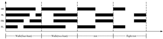
Figure 1.
The black block indicates that the single leg of the quadruped robot is in the support phase. FL: Front Left Leg. FR: Front Right Leg. HL: Hind Left Leg. HR: Hind Right Leg.
The main contributions of this paper are: (a) An MPC-based method for selecting the foot location is proposed based on the LIP model and the dynamics model of the quadruped robot, which solves the problem of large posture oscillation during gait transitioning in different gait periods. (b) UPMPC is able to complete some of gait transitioning that cannot be done by the HF. (c) UPMPC selects the foot location based on the predicted future state, which improves the overall adaptability of the quadruped robot.
The paper is organized as follows. Section 3 presents the overall control architecture of the quadruped robot. The composition of MPC and the functions of the UPMPC are briefly demonstrated. A detailed mathematical description of UPMPC is illustrated in Section 4. A comparison of UPMPC with HF in a simulation environment is given in Section 5. Section 6 is a summary of the whole text.
3. Control Architecture
The control method used in this paper is MIT’s Convex MPC [4]. The overall control block diagram [4] is shown in Figure 2.
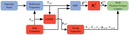
Figure 2.
The red block indicates the control frequency at 0.5 kHz, the blue block indicates the control frequency at 30 Hz, and the green block indicates the control frequency at 4.5 kHz [4]. is the reference state of the robot. is the estimated state of the robot. is the desired foot location in the world coordinate system. is the GRFs in the world coordinate system and is the GRFs in the ontology coordinate system. denotes the PD control parameters of the joint, the feedforward force, the desired foot location under the body coordinate system, and the desired foot velocity in the body coordinate system, respectively. The swing leg is position controlled and the control effect of the joint is adjusted according to the PD control gain .
Based on Convex MPC, the UPMPC for selecting the foot location is added. Operator Input is the user input for commands such as gait, speed and direction. Reference Trajectory generates a reference state for the robot based on user input, such as the robot’s pose and speed. State Estimator estimates the robot’s state based on the sensor data. Swing Trajectory is used in three main purposes: selection of swing legs, determination of swing time and generation of swing trajectory. Swing Trajectory generates the desired swing trajectory for the swing leg to track based on the reference foot location input by the UPMPC. MPC outputs the desired GRFs based on the output of Reference Trajectory. The UPMPC selects the foot location of the swing leg.
The UPMPC input variables are the desired state, the current estimated state and the GRFs planned by MPC when switching from the swing phase to the support phase. The output variables are the desired foot location. Using the LIP model and dynamics model of the robot, the selection of the foot location is simplified to a QP problem. The desired result is obtained from the solution of the QP problem. The detailed mathematical derivation and introduction are in shown in Section 4.
4. Foot Location Selection Based on MPC
The expression for the HF is shown in Equation (1).
is the desired foot location of the quadruped robot. is the location of the hip projected onto the ground. is the current speed of the COM. is the time the foot will spend on the ground. is the desired speed of the COM. All the variables above are in the world coordinate system. is the gain of the difference between and . Due to the characteristics of different gaits, the posture of the quadruped robot after gait transitioning will have a large offset from the steady state. In this case, HF may choose a foot location that is not conducive to the stability of the quadruped robot’s posture in order to correct the velocity offset. If it is desired to do a better job of transitioning between several different gaits, a heuristic gain value needs to be determined for each gait. Therefore, a new way of foot location planning is needed to enable gait transitioning of quadruped robots in multiple gaits with a single set of parameters. The variables used in the equations below are shown in Figure 3.
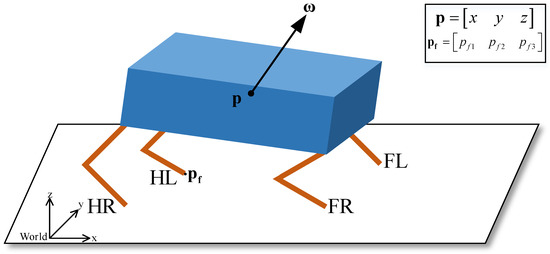
Figure 3.
A model of the quadurped robot is shown in the figure. The World in the bottom left corner of the diagram indicates the defined world coordinate system. The black frame in the top right corner indicates the composition of the variables labelled in the model. is the position of the robot’s foot end. is the position of the robot’s COM. is the ground reaction force. All the variables mentioned are in the world coordinate system.
The LIP model has been widely used in bipedal robot motion [17,18]. The simplified LIP model allows better planning of the bipedal robot’s foot location. LIP can also be applied to quadrupedal robots [19,20]. With the virtual leg concept, a quadrupedal robot can be equated to a bipedal robot. At this point the quadruped robot can also apply the LIP model to plan the foot location. Therefore, the LIP model can be used to predict the velocity of the quadruped robot. In a single-point support, the COM is pushed by the support foot. The forward acceleration is driven by the difference between the support foot position and the COM position x.
where represents the position of the supporting foot in the x-axis direction in the world coordinate system, and x, and represent the position of the COM, the acceleration in the x-axis and the height in the z-axis in the world coordinate system, respectively. g is the acceleration of gravity in the z-axis in the world coordinate system. With the height of COM constant, the value of is determined only by x and .
The lateral acceleration is driven by the difference between the position of support foot and the position y of the COM.
where represents the position of the supporting foot in the y-axis direction in the world coordinate system, and y and represent the position of the COM and the acceleration in the y-axis under the world coordinate system, respectively. Let the COM state be , then the equation of state is shown in Equation (4).
is the robot’s current state. Extending the COM state to , is the position of the COM in the world coordinate system. is the velocity of the COM in the world coordinate system. The position of the supportting foot is extended to the coordinates of the foot in the world coordinate system during the motion of the quadruped robot. The equation of state is shown in Equation (6).
where is the position of the foot in the world coordinate system. and are the coordinates of the foot i and the GRFs in the world coordinate system, respectively. In the LIP model, the choice of the foot location affects the velocity of the COM, but not the height of the COM. Equation (10) is used to determine the swing leg.
The presence of GRFs makes the location of the foot affect the COM posture. Therefore, the choice of foot location needs to consider the effect on the velocity and the posture.
The dynamics of a quadruped robot rotating around the COM in the world coordinate system is shown in Equation (11).
where is the robot’s inertia tensor, is the angular velocity of the robot. is the vector between the position of the foot end and the COM. When is small, the left side of Equation (11) can be approximated with:
Converting the right-hand side of Equation (11) to a representation of the COM position and the foot position in the world coordinate system.
Then Equation (11) can be converted to:
where is the GRFs of MPC planning when switching from the swing phase to the support phase in the previous period. The equation of state of the system is
where , . Discretize Equation (15) using a zero-order retainer:
Combining the current COM state , the GRFs planned by the MPC when the foot touched the ground in the previous period and the reference state of the robot, the location of the foot is determined according to Equation (18). Let the desired foot location be . After the foot touches the ground without slipping, the position in the world coordinate system does not change. The equation for the change of the state for the next N steps can be obtained.
The control problem can be transformed into the selection of the foot location that the robot will achieve the desired state at step N.
Both and are adjustable weight matrices and semi-positive definite. Equation (23) selects the foot that is currently in the swing period. By using Equations (19) and (20) can be converted into the following quadratic optimization form.
where , . By limiting the foot location of each time step to be equal, the dimension of the matrix to be computed is greatly reduced and the efficiency of the computation is improved. The dimensionality of the final matrices and vector is independent of the prediction length and is only related to the number of variables. Therefore, it can greatly reduce the amount of computation to improve the computation speed and increase the frequency of prediction.
is the acceleration of gravity. Equations (11) and (25) form the complete dynamics model of the quadruped robot. In Equation (11), angular acceleration is determined by the foot location and GRFs. The GRFs also determines the linear acceleration in Equation (25). The user not only wants the quadruped robot to be able to keep up with the desired speed, but also to ensure that the posture is stable around the desired value. This places demands on both linear and angular acceleration. The MPC controller will select the GRFs based on Equations (11) and (25) and the foot location. Therefore, the choice of foot location will directly influence the outcome of the GRFs.
The HF selects the foot location only according to the current state so that the gain value greatly affects the result. The UPMPC considers not only the current state but also the influence of the foot location on the future state. It improves adaptability by selecting a foot location where the future state is more in line with the desired one, rather than just based on the current state. Therefore, the UPMPC can adapt to multiple gaits and complete gait transitioning between different periods.
5. Results
5.1. Simulation Setup
The proposed UPMPC is validated based on the simulation platform of MIT [21]. The simulation environment is shown in Figure 4 below. It is based on Ubuntu 18.04. MIT’s Mini Cheetah is used [5] as the verification model for the algorithm. In which the robot with 12 degrees of freedom weighs 9 kg [5], the friction between the foot and the ground is 0.4. All of the joints are motor driven and torque controlled. LCM is used for communication between the simulation environment and the control interface. LCM is lightweight real-time communication software [22]. In this paper, qpOASES [23] is used as a solver for the QP problem. qpOASES is specifically used to solve the MPC quadratic optimization problem. The walking gait chosen in this paper is two-beat walking, so the diagonal leg of walking, trotting and flight trotting can be equated to a virtual leg. At this point, the quadruped robot is equivalent to a bipedal robot. Furthermore, the LIP model can be applied. The control frequency of UPMPC is 0.5 kHz.
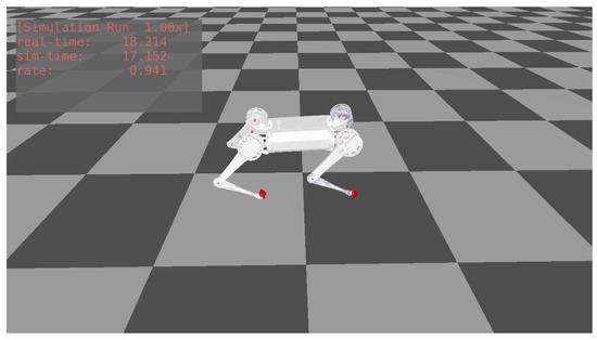
Figure 4.
The model in simulation environment is the Mini Cheetah. The real-time in the upper left corner indicates the time of the real world. The sim-time represents the time in the simulation environment. The rate denotes the simulation rate.
During the simulation experiments, the control parameters of MPC are kept constant. The prediction length of MPC method is 10 steps in all three gaits. The time length of each step is 0.03 s. The prediction time is 0.3 s and the control frequency is 33 Hz. The prediction length of UPMPC is three steps. The time length of each step is 0.03 s. None of the parameters of the HF or UPMPC are changed during the motion. The periods of walking, trotting and flight trotting are 0.6 s, 0.42 s and 0.3 s, respectively. The duty cycle of walking, trotting and flight trotting are 0.6, 0.5 and 0.3, respectively. Each gait transitioning interval is 3 s. The swing leg is planned with a Bessel curve. Figure 5 shows the COT [24] of three gaits. COT is used to indicate the energy consumption level of the quadruped robot.
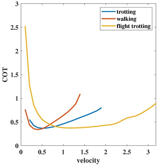
Figure 5.
COT of walking, trotting and flight trotting at different speeds, respectively.
The three curves in Figure 5 represent the different gaits. The horizontal axis coordinate corresponding to the rightmost end of each curve indicates the maximum speed that can be achieved at the current gait. According to the curves in the image, the energy consumption at various speeds for different gaits is variable. To reduce energy consumption or to meet task requirements, the robot needs to transitioning between multiple gaits. Because gait transitioning is performed at multiple speeds, the experiment is divided into five parts to verify the performance of UPMPC:
- Transitioning between three gaits at the speed of 0.4 m/s;
- Transitioning between three gaits at the speed of 0.8 m/s;
- Transitioning between trotting and flight trotting at the speed of 1.2 m/s;
- Transitioning between trotting and flight trotting at the speed of 1.6 m/s;
- Movement of trotting gait using the UPMPC
At 0.4 m/s, walking has lower energy consumption. Higher than this speed, the energy consumption of trotting is lower than walking. Transitioning between trotting and walking at this speed can complete the transitioning of energy consumption smoothly. At this time, flight trotting energy consumption is higher, but can have greater acceleration. Flight trotting is indispensable when the robot wants to accelerate quickly from low speed to high speed. Therefore, it is of great importance to perform the transitioning between the three gaits.
At 0.8 m/s, it is the approximate speed at which the trotting and flight trotting COT curves appear to intersect. Greater than this speed, flight trotting energy consumption is less than trotting energy consumption. Flight trotting can accelerate to very fast speed in the short time while walking can ensure posture stability at a certain speed. Therefore, flight trotting and walking transitioning at this speed are equally relevant for applications.
For walking, 1.2 m/s and 1.6 m/s are already quite large speed of movement, very close to the maximum speed in that gait, which itself is already not moving stably enough. Feet in swing may collide with feet lifting off the ground sometimes. Furthermore, the COT in this gait is already much larger than trotting and flight trotting. Therefore, transitioning between trotting or flight trotting and walking at this speed lacks practical meaning. Only the gait transitioning between trotting and flight trotting is considered.
To eliminate the effect of incidental factors, multiple gait transitioning is performed at a given speed during the transitioning process. During the motion of a quadruped robot, the posture change is closely related to the stability of the control. With small variations in posture, the quadruped robot performs better in actual motion. Ideally, a quadruped robot is most stable when the posture is at the desired value and does not change during motion. Therefore, comparing the change in posture at the time of gait transitioning and throughout the gait transitioning process gives a good indication of how well the foot location planning method works. With the control algorithm unchanged, the choice of foot location affects the planning result of MPC in gait transitioning, which in turn influences the posture control of the quadruped robot. The posture is the result of the combined effect of force and foot location. The advantages and disadvantages of the two methods can be determined by posture changes and foot-end forces. Because the selected gaits are all symmetrical, the force change at the foot end of one leg can better reflect the planning result of MPC. The effectiveness and superiority of the UPMPC can be better demonstrated by integrating the results of force planning and posture change. Finally, the posture changes in trotting are shown to demonstrate that UPMPC can also get good results in a single gait.
5.2. UPMPC vs. HF
In this section, the peak value and the mean of absolute value are used to compare the advantages and disadvantages of the two methods. The peak value is able to reflect the stability of the posture after transitioning. Smaller peak indicates less posture oscillation and better stability. The mean of absolute value gives a better evaluation to the change in posture throughout the process and eliminates the effect of positive and negative values. A smaller mean of absolute value of the posture indicates that the quadruped robot recovers from postural oscillations more quickly after a gait transitioning or the change in posture is relatively small over the whole time. If the mean of absolute value is large, the quadruped robot is unable to return to a stable state more quickly after a gait transitioning, or has a large oscillation over the whole time.
The numbers marked in the figures below are the times at which the gait transitioning takes place. The peak value used is the maximum value of the posture for the duration after the gait transitioning has occurred and before the next starts. There is a time delay between the peak values and the transitioning point, as the quadruped robot needs a very short amount of time after the gait transitioning to reach its most unstable moment. This part of the time is not negligible. Therefore, it will be seen that there is a lag between the time of the transitioning point and the time of peak values.
Figure 6 is the gait transitioning between trotting and walking at 0.4 m/s. The gait transitioning using the HF in Figure 6a fails directly and using the UPMPC in Figure 6b succeeds despite facing a large posture oscillation. In Figure 6a, a large posture oscillation has happened during the gait transitioning but the foot location of the HF planning cannot cope with this situation. It makes the roll and yaw deviate more and more from the stable position, leading to the posture divergence and gait transitioning failure. The posture change is not so clear in Figure 6a,b. In Figure 6e, it becomes clear. In this graph the peak of the posture after the gait transitioning is shown. The numbers 1, 2 and 3 stand for roll, pitch and yaw, respectively. It is clear from Figure 6e that the gait transitioning using the HF faces a large posture peak after the transitioning and far exceeds that of the UPMPC. This is more than the controller can steadily control, making the system falter and the transitioning fail. In Figure 6b,e, with the controller unchanged, the UPMPC planned foot location effectively reduces the peak values of the posture comparing with the HF, allowing the posture to return to near the stable value. Even if the transitioning results in a large posture change, the UPMPC is able to help keep the robot moving stably by planning a good foot location. Figure 6c,d shows the foot-end force planned by MPC for the left front leg foot of the quadruped robot during the transitioning process. Figure 6f shows the comparison of the peak force at the foot end after transitioning. The difference in peak force is not so clear from Figure 6c,d. However, in Figure 6f, a huge difference is shown. The huge force may cause unnecessary vibration and instability. It is not desirable that the peak of the foot-end force is too large if the gait transitioning can be done. This is because it will have a large impact on the posture and affects the stability of the quadruped robot after gait transitioning. As can be seen from Figure 6f, the forces required by the robot using UPMPC are much smaller during gait transitioning. The quadruped robot regains stability in its posture by the combined effect of force and foot-end position. In Figure 6f, the HF uses a greater force to try to restore stability, but the gait transitioning still fails. In contrast, the UPMPC successfully completes the gait transitioning with less force.
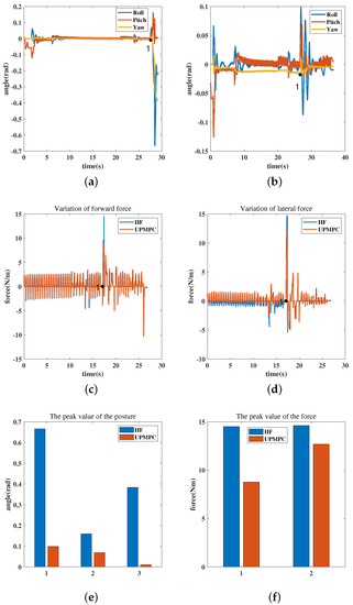
Figure 6.
The figure shows the posture and GRFs of trotting in a gait transitioning to walking at 0.4 m/s. The number 1 in (a–d) indicate gait transitioning occuring. The horizontal coordinate of the number 1 in the diagram represents the exact time of the transitioning. The transitioning process is: trotting (0–27.6 s), walking (27.6-final). (c,d) Only capture the GRFs near the transitioning point to facilitate analysis of the forces, so the transitioning time is not consistent with (a,b). All data in the plots are from the same dataset. (a) Posture change using the HF at 0.4 m/s gait transitioning. (b) Posture change using the UPMPC at 0.4 m/s gait transitioning. (c) Change in forward force at 0.4 m/s during gait transitioning. (d) Change in lateral force at 0.4 m/s during gait transitioning. (e) Comparison of the peak values of roll, pitch and yaw for the two methods after transitioning. The numbers 1, 2 and 3 on the horizontal axis in the graph represent roll, pitch and yaw, respectively. (f) Comparison of peak values after transitioning for forward and lateral forces under both methods. The numbers 1 and 2 on the horizontal axis in the diagram represent forward and lateral forces, respectively.
These would suggest that the foot location chosen by the UPMPC is far superior to the HF. Gait transitioning is accomplished with less foot-end force and less posture oscillation. UPMPC shows a great advantage over HF in completing the gait transitioning between trotting and walking.
Figure 7 is the posture change during gait transitioning between flight trotting and walking at 0.8 m/s. The transitioning points are marked by the numbers 1, 2, 3, 4 and 5 in the figure. In Figure 7a, the change of roll using UPMPC is basically consistent with HF. All have oscillation after the transitioning. In Figure 7b, the numbers 1, 2, 3, 4, 5 show the peak of the posture after the gait transitioning. A distinct difference between the two methods can be seen in in Figure 7b. In this figure, the peak of roll using the UPMPC is smaller than that of the HF, except for the fourth gait transitioning. The location of the foot chosen by the UPMPC enables a smaller roll peak after transitioning. This indicates that the quadruped robot with the UPMPC is more stable after switching. The number 6 represents the mean of absolute value of the roll. Smaller mean of the absolute values can indicate that the quadruped robot is more stable throughout the whole transitioning process. In Figure 7b, the mean of absolute value of roll using the HF is significantly larger than that using the UPMPC. The roll with the less oscillations over the whole time has the small mean of the absolute values. Combining the mean of absolute value and the peak values, the UPMPC has better control over roll. In Figure 7c, the curves of the two methods overlap highly. In Figure 7d, both the peak values and the mean of absolute value of pitch at the gait transitioning using UPMPC are smaller. Therefore, the UPMPC has better control of the pitch. In Figure 7e, yaw drifts regardless of the foot location planning method. As the number of transitioning accumulates, the yaw drift of UPMPC is smaller than that of the HF in Figure 7e. UPMPC has better control of yaw during gait transitioning. Comparing Figure 7b,d, the good control of yaw by UPMPC does not come at the expense of roll and pitch. Figure 8 is the foot-end force change during gait transitioning between flight trotting and walking at 0.8 m/s. Figure 8a,c show the force planned by MPC for the foot-end of the left front leg during the transitioning process. In Figure 8b, the force peaks of the UPMPC are significantly smaller in the second, third and fourth gait transitioning. The HF has a slightly smaller force peak in the first and fifth gait transitioning. It is not possible to distinguish exactly which method has the smaller mean of absolute values. The forward forces required by the robot are nearly the same for both methods over the whole time. In Figure 8d, the peak using the HF is smaller than that of UPMPC over the whole time. However, there is no difference in the mean of absolute value between the two methods. This means that both methods require essentially the same size force over the whole time. There is no considerable difference between the two methods in regards to forward forces or lateral forces. Combined with the change of posture, the UPMPC uses the same force to achieve smaller posture peak and mean of absolute values of posture over the whole time. Therefore, the UPMPC enables better control of posture. The UPMPC helps the quadruped robot to perform better in gait transitioning tasks at 0.8 m/s. The overall oscillations in posture are also smaller. However, it still cannot avoid the oscillation of posture at the moment of transitioning. The better effect of UPMPC has been demonstrated.
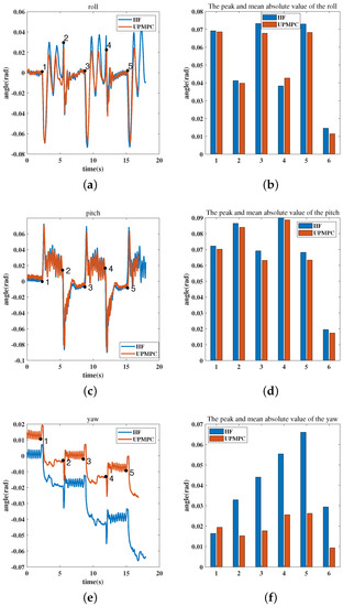
Figure 7.
The figure shows the posture changes in gait transitioning between flight trotting and walking at 0.8 m/s. The numbers 1, 2, 3, 4 and 5 in (a,c,e) indicate gait transitioning occuring. The horizontal coordinate of these numbers in the diagram represents the exact time of the transitioning. The transitioning process is: flight trotting (0–2.27 s (number 1)), walking (2.27–5.27 s (number 2)), flight trotting (5.27–8.77 s (number 3)), walking (8.77–11.81 s (number 4)), flight trotting (11.81–15.20 s (number 5)) and walking (15.20-final). The numbers 1, 2, 3, 4 and 5 in (b,d,f) denote the peak values of the corresponding posture (roll, pitch or yaw) after the gait transitioning. Furthermore, the number 6 indicates the mean of the absolute value of the corresponding posture over the whole time. (a) Changes in roll during gait transitioning at 0.8 m/s. (b) Comparison of the peak values of roll after transitioning and mean of the absolute values of roll in the whole time for the two methods at 0.8 m/s. (c) Changes in pitch during gait transitioning at 0.8 m/s. (d) Comparison of the peak values of pitch after transitioning and mean of the absolute values of pitch in the whole time for the two methods at 0.8 m/s. (e) Changes in yaw during gait transitioning at 0.8 m/s. (f) Comparison of the peak values of yaw after transitioning and mean of the absolute values of yaw in the whole time for the two methods at 0.8 m/s.
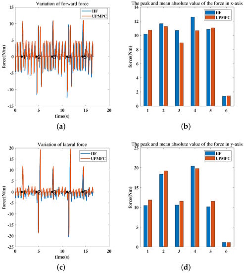
Figure 8.
The figure shows the force changes in gait transitioning between flight trotting and walking at 0.8 m/s. The numbers 1, 2, 3, 4 and 5 in (a,c) indicate gait transitioning occuring. The horizontal coordinate of these numbers in the diagram represents the exact time of the transitioning. The transitioning process is: flight trotting (0–1.37 s (number 1)), walking (1.37–4.54 s (number 2)), flight trotting (4.54–7.86 s (number 3)), walking (7.86–11.05 s (number 4)), flight trotting (11.05–14.33 s (number 5)) and walking (14.33-final). The numbers 1, 2, 3, 4 and 5 in (b,d) denote the peak values of the corresponding forward forces or lateral forces after the gait transitioning. Furthermore, the number 6 indicates the mean of the absolute value of the corresponding forces over the whole time. (a) Change in forward force at 0.8 m/s. (b) Comparison of the peak values of forward force after transitioning and mean of the absolute values of forward force in the whole time for the two methods at 0.8 m/s. (c) Change in lateral force at 0.8 m/s. (d) Comparison of the peak values of lateral force after transitioning and mean of the absolute values of lateral force in the whole time for the two methods at 0.8 m/s.
Figure 9 is the posture change during gait transitioning between flight trotting and trotting at 1.2 m/s. The transitioning points are marked by the numbers 1, 2, 3, 4 and 5 in the figure. In Figure 9a, many parts are overlapped. At three transitioning points, the peak of the roll using UPMPC is slightly larger than that of HF in Figure 9c. However, the HF does not show a clear advantage over the UPMPC in reducing the peaks values. The mean of absolute value of the two methods is basically the same. For a slightly larger peak values than the HF, the UPMPC has the same mean of absolute value. It shows that the UPMPC allows the quadruped robot to recover stable from the postural oscillation of the transitioning more quickly. Despite the small peak values, the HF requires a longer time of posture oscillation to remove the effects of the transitioning. Therefore, it cannot be stated which method is really better for roll control. In Figure 9e, both methods have a large change in pitch at the instant of transitioning. The pitch using UPMPC has a smaller peak. It can be clearly seen from Figure 9b. At the same time, the mean of absolute values of pitch using the UPMPC is also smaller than that using the HF. Therefore, the UPMPC has better control for pitch. In Figure 9d, the yaw of both methods has some variation. In contrast to the UPMPC, HF does not control yaw well. Yaw gradually deviates from the stable value as gait transitioning occurs. The yaw using UPMPC also deviates, but its deviation under multiple gait transitioning is much smaller than HF in Figure 9f. Thus, the UPMPC has better control for yaw. Stability of posture is a prerequisite for the stable movement of a quadruped robot. Figure 10a,b shows the foot-end force of the left front leg planned by the MPC during the transitioning process. In Figure 10a, the vast majority of the curves from both methods overlap. A clear feedback is also obtained in Figure 10c. It was not possible to clearly determine which method had a smaller peak value of the forward force after gait transitioning. The mean of absolute values are also essentially the same. The forces are essentially the same under both methods. From the peak values, the lateral forces planned by UPMPC become significantly smaller than those of HF in Figure 10d. During the whole transitioning process, the lateral forces of HF are significantly greater than those of the UPMPC. Comparing to HF, the robot with the UPMPC has less posture change during gait transitioning, along with same forward forces and less lateral forces over the whole time at the speed of 1.2 m/s. The gait transitioning task is done better by the UPMPC. This indicates that the UPMPC selects a better location for the landing point. Combining the forces and posture, UPMPC’s results are much better than HF’s.
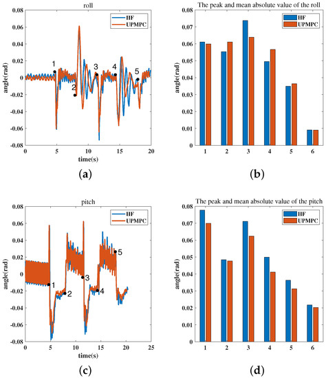
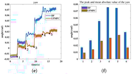
Figure 9.
The figure shows the posture changes in gait transitioning between trotting and flight trotting at 1.2 m/s. The numbers 1, 2, 3, 4 and 5 in (a,c,e) indicate gait transitioning occuring. The horizontal coordinate of these numbers in the diagram represents the exact time of the transitioning. The transitioning process is: trotting (0–4.66 s (number 1)), flight trotting (4.66–7.87 s (number 2)), trotting (7.87–11.36 s (number 3)), flight trotting (11.36–14.38 s (number 4)), trotting (14.38–17.88 s (number 5)) and flight trotting (17.88-final). The numbers 1, 2, 3, 4 and 5 in (b,d,f) denote the peak values of the corresponding posture (roll, pitch or yaw) after the gait transitioning. Furthermore, the number 6 indicates the mean of the absolute value of the corresponding posture over the whole time. (a) Changes in roll during gait transitioning at 1.2 m/s. (b) Comparison of the peak values of roll after transitioning and mean of the absolute values of roll in the whole time for the two methods at 1.2 m/s. (c) Changes in pitch during gait transitioning at 1.2 m/s. (d) Comparison of the peak values of pitch after transitioning and mean of the absolute values of pitch in the whole time for the two methods at 1.2 m/s. (e) Changes in yaw during gait transitioning at 1.2 m/s. (f) Comparison of the peak values of yaw after transitioning and mean of the absolute values of yaw in the whole time for the two methods at 1.2 m/s.
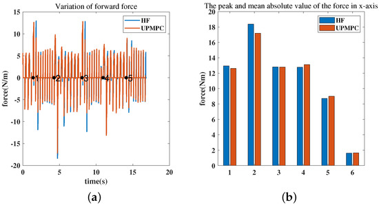
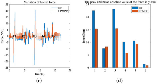
Figure 10.
The figure shows the force changes in gait transitioning between flight trotting and trotting at 1.2 m/s. The numbers 1, 2, 3, 4 and 5 in (a,c), indicate gait transitioning occuring. The horizontal coordinate of these numbers in the diagram represents the exact time of the transitioning. The transitioning process is: trotting (0–1.4 s (number 1)), flight trotting (1.4–4.26 s (number 2)), trotting (4.26–8.08 s (number 3)), flight trotting (8.08–10.94 s (number 4)), trotting (10.94–14.11 s (number 5)) and flight trotting (14.11-final). The numbers 1, 2, 3, 4 and 5 in (b,d) denote the peak values of the corresponding forward forces or lateral forces after the gait transitioning. Furthermore, the number 6 indicates the mean of the absolute value of the corresponding forces over the whole time. (a) Change in forward force at 1.2 m/s gait transitioning. (b) Comparison of the peak values of forward force after transitioning and mean of the absolute values of forward force in the whole time for the two methods at 1.2 m/s. (c) Change in lateral force at 1.2 m/s gait transitioning. (d) Comparison of the peak values of lateral force after transitioning and mean of the absolute values of lateral force in the whole time for the two methods at 1.2 m/s.
5.3. Walk with a Fixed Gait
The UPMPC can also be used for walking with a fixed gait. Let the gait be trotting and the foot location planning method be UPMPC. In this gait the quadruped robot accelerates from stepping in place to 1.6 m/s. Each speed increase is 0.1 m/s with time interval of 30 gait periods (12.6 s). The roll, pitch and yaw changes during this process are shown in Figure 11.
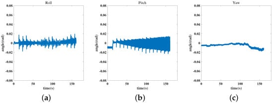
Figure 11.
(a) The change of roll in trottting. (b) The change of pitch in trottting. (c) The change of yaw in trottting.
The quadruped robot has a small spike at each acceleration and the amplitude of the oscillation increases as the speed increases. Yaw has deviated from the stable value. However, it basically oscillates back and forth around the stable value. The peak values of posture has not yet exceeded rad which is so small that it can be ignored. With the same control method, the use of UPMPC also allows the quadruped robot to advance at a uniform speed and accelerate steadily. Therefore, UPMPC can be applied not only in the process of gait transitioning, but also in the planning of foot location under fixed gait.
5.4. Discussion
Figure 12 is the gait transitioning between trotting and walking at 0.8 m/s. This figure is different from Figure 6a. The gait transitioning using the HF in Figure 12a fails. The three postures after the transitioning are a straight line with no change, indicating that the quadruped robot is at stationary position. There is no command given after transitioning in the simulation. Thus, the gait transitioning has failed and the robot falls to the ground. It fails because of the large posture changes generated after the gait transitioning and the foot-end forces do not provide good control of the posture. The gait transitioning using the UPMPC in Figure 12b succeeds. However, the posture still face a huge oscillation. The control method for the quadruped robot is MPC all the time. Despite the greater foot end forces, the UPMPC planned foot location can perform gait transitioning tasks together with the controller. Although the force is less, the gait transitioning using the HF cannot be completed. It indicates that the foot location chosen by HF at this point is not reasonable. The foot location and foot-end forces under the HF can not correct for postural deviations. The HF cannot cope with this gait transitioning. Therefore the UPMPC’s choice of foot location is still preferable to HF. The rest of the simulation results are in the Appendix A.
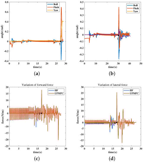
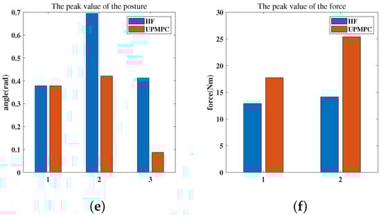
Figure 12.
The figure shows the posture and GRFs of trotting in a gait transitioning to walking at 0.8 m/s. The number 1 in (a–d) indicate gait transitioning occuring. The horizontal coordinate of the number 1 in the diagram represents the exact time of the transitioning. The transitioning process is: trotting (0–28.3 s), walking (28.3-final). (c,d) only capture the GRFs near the transitioning point to facilitate analysis of the forces, so the transitioning time is not consistent with (a,b). All data in the plots are from the same dataset. (a) Posture change using the HF at 0.8 m/s gait transitioning. (b) Posture change using the UPMPC at 0.8 m/s gait transitioning. (c) Change in forward force at 0.8 m/s during gait transitioning. (d) Change in lateral force at 0.8 m/s during gait transitioning. (e) Comparison of the peak values of roll, pitch and yaw for the two methods after transitioning. The numbers 1, 2 and 3 on the horizontal axis in the graph represent roll, pitch and yaw, respectively. (f) Comparison of peak values after transitioning for forward and lateral forces under both methods. The numbers 1 and 2 on the horizontal axis in the diagram represent forward and lateral forces, respectively.
6. Conclusions
Combining multiple gaits transitioning at various speeds, UPMPC performs better than the HF in all cases. In particular, the gait transitioning between trotting and walking cannot be done by the HF but can be done by UPMPC. Furthermore, it has much better control over yaw and pitch than HF. At most gait transitioning, the mean of absolute values of roll under UPMPC is smaller. UPMPC with fixed parameters is able to accommodate gait transitioning between multiple gaits at a variety of speeds.
Despite the use of a simplified model to describe the kinematics and dynamics of the quadruped robot, the UPMPC-planned foot location still meets the requirements for gait transitioning and is better than HF. The use of the uniform foot location not only speeds up the solution, but also converts the problem to be solved into a QP form with a smaller matrix. The coordinates of the foot in the world coordinate system are used as the optimization solution variable more in line with the actual situation. Due to the good migration of the used platform, it is believed that UPMPC can be applied in real systems to meet the need of gait transitioning on real world.
Author Contributions
Conceptualization, methodology and writing—original draft preparation, X.L.; writing—review and editing, L.L., H.A. and H.M. All authors have read and agreed to the published version of the manuscript.
Funding
This work was funded by National Science Foundation of China (No. 61903131) and Outstanding Youth of Department of Education of Hunan Province (No. 20B096) and the China Postdoctoral Science Foundation (No. 2020M683715).
Institutional Review Board Statement
Not applicable.
Informed Consent Statement
Not applicable.
Data Availability Statement
The simulation code can be downloaded in https://github.com/lxm-1/Mini-Cheetah.git accessed on 23 August 2021.
Conflicts of Interest
The authors declared no potential conflict of interest with respect to the research, authorship, and/or publication of this article.
Appendix A
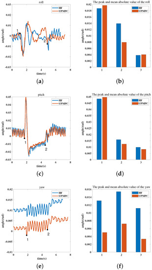
Figure A1.
The figure shows the posture changes in gait transitioning between trotting and flight trotting at 0.4 m/s. The numbers 1 and 2 in (a,c,e) indicate gait transitioning occuring. The horizontal coordinate of these numbers in the diagram represents the exact time of the transitioning. The transitioning process is: trotting (0–1.80 s (number 1)), flight trotting (1.80–4.76 s (number 2)) and trotting (4.76-final). The numbers 1 and 2 in (b,d,f) denote the peak values of the corresponding posture (roll, pitch or yaw) after the gait transitioning. Furthermore, the number 3 indicates the mean of the absolute values of the corresponding posture over the whole time. (a) Changes in roll during gait transitioning at 0.4 m/s. (b) Comparison of the peak values of roll after transitioning and mean of the absolute values of roll in the whole time for the two methods at 0.4 m/s. (c) Changes in pitch during gait transitioning at 0.4 m/s. (d) Comparison of the peak values of pitch after transitioning and mean of the absolute values of pitch in the whole time for the two methods at 0.4 m/s. (e) Changes in yaw during gait transitioning at 0.4 m/s. (f) Comparison of the peak values of yaw after transitioning and mean of the absolute values of yaw in the whole time for the two methods at 0.4 m/s.
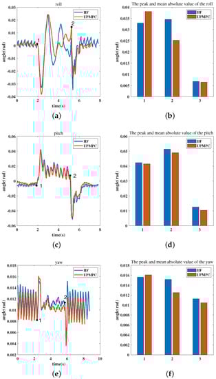
Figure A2.
The figure shows the posture changes in gait transitioning between flight trotting and walking at 0.4 m/s. The numbers 1 and 2 in (a,c,e) indicate gait transitioning occuring. The horizontal coordinate of these numbers in the diagram represents the exact time of the transitioning. The transitioning process is: flight trotting (0–1.88 s (number 1)), walking (1.88–5.12 s (number 2)) and flight trotting (5.12-final). The numbers 1 and 2 in (b,d,f) denote the peak values of the corresponding posture (roll, pitch or yaw) after the gait transitioning. Furthermore, the number 3 indicates the mean of the absolute value of the corresponding posture over the whole time. (a) Changes in roll during gait transitioning at 0.4 m/s. (b) Comparison of the peak values of roll after transitioning and mean of the absolute values of roll in the whole time for the two methods at 0.4 m/s. (c) Changes in pitch during gait transitioning at 0.4 m/s. (d) Comparison of the peak values of pitch after transitioning and mean of the absolute values of pitch in the whole time for the two methods at 0.4 m/s. (e) Changes in yaw during gait transitioning at 0.4 m/s. (f) Comparison of the peak values of yaw after transitioning and mean of the absolute values of yaw in the whole time for the two methods at 0.4 m/s.
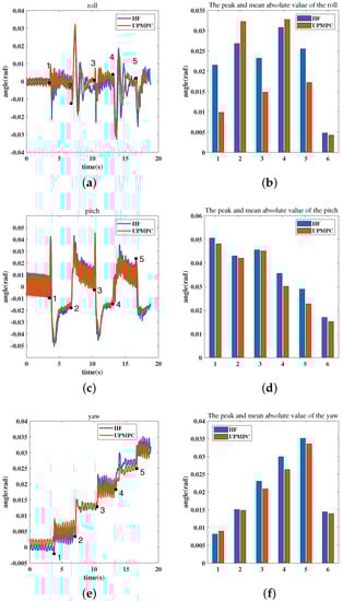
Figure A3.
The figure shows the posture changes in gait transitioning between trotting and flight trotting at 0.8 m/s. The numbers 1, 2, 3, 4 and 5 in (a,c,e) indicate gait transitioning occuring. The horizontal coordinate of these numbers in the diagram represents the exact time of the transitioning. The transitioning process is: trotting (0–3.48 s (number 1)), flight trotting (3.48–6.77 s (number 2)), trotting (6.77–10.28 s (number 3)), flight trotting (10.28–13.10 s (number 4)), trotting (13.10–16.61 s (number 5)) and flight trotting (16.61-final). The numbers 1, 2, 3, 4 and 5 in (b,d) denote the peak values of the corresponding posture (roll, pitch or yaw) after the gait transitioning. Furthermore, the number 6 indicates the mean of the absolute value of the corresponding posture over the whole time. (a) Changes in roll during gait transitioning at 0.8 m/s. (b) Comparison of the peak values of roll after transitioning and mean of the absolute values of roll in the whole time for the two methods at 0.8 m/s. (c) Changes in pitch during gait transitioning at 0.8 m/s. (d) Comparison of the peak values of pitch after transitioning and mean of the absolute values of pitch in the whole time for the two methods at 0.8 m/s. (e) Changes in yaw during gait transitioning at 0.8 m/s. (f) Comparison of the peak values of yaw after transitioning and mean of the absolute values of yaw in the whole time for the two methods at 0.8 m/s.
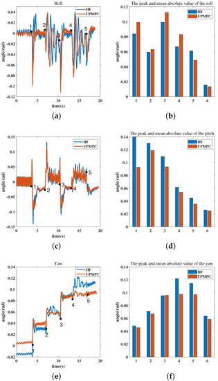
Figure A4.
The figure shows the posture changes in gait transitioning between trotting and flight trotting at 1.6 m/s. The numbers 1, 2, 3, 4 and 5 in (a,c,e) indicate gait transitioning occuring. The horizontal coordinate of these numbers in the diagram represents the exact time of the transitioning. The transitioning process is: trotting (0–3.57 s (number 1)), flight trotting (3.57–6.79 s (number 2)), trotting (6.79–10.27 s (number 3)), flight trotting (10.27–13.09 s (number 4)), trotting (13.09–16.72 s (number 5)) and flight trotting (16.72-final). The numbers 1, 2, 3, 4 and 5 in (b,d) denote the peak values of the corresponding posture (roll, pitch or yaw) after the gait transitioning. Furthermore, the number 6 indicates the mean of the absolute value of the corresponding posture over the whole time. (a) Changes in roll during gait transitioning at 1.6 m/s. (b) Comparison of the peak values of roll after transitioning and mean of the absolute values of roll in the whole time for the two methods at 1.6 m/s. (c) Changes in pitch during gait transitioning at 1.6 m/s. (d) Comparison of the peak values of pitch after transitioning and mean of the absolute values of pitch in the whole time for the two methods at 1.6 m/s. (e) Changes in yaw during gait transitioning at 1.6 m/s. (f) Comparison of the peak values of yaw after transitioning and mean of the absolute values of yaw in the whole time for the two methods at 1.6 m/s.
References
- Hoyt, D.F.; Taylor, C.R. Gait and the energetics of locomotion in horses. Nature 1981, 292, 239–240. [Google Scholar] [CrossRef]
- Xi, W.; Yesilevskiy, Y.; Remy, C.D. Selecting gaits for economical locomotion of legged robots. Int. J. Robot. Res. 2016, 35, 1140–1154. [Google Scholar] [CrossRef]
- Raibert, M.H. Legged Robots That Balance; MIT Press: Cambridge, MA, USA, 1986. [Google Scholar]
- Di Carlo, J.; Wensing, P.M.; Katz, B.; Bledt, G.; Kim, S. Dynamic locomotion in the mit cheetah 3 through convex model-predictive control. In Proceedings of the 2018 IEEE/RSJ International Conference on Intelligent Robots and Systems (IROS), Madrid, Spain, 1–5 October 2018; pp. 1–9. [Google Scholar]
- Katz, B.; Di Carlo, J.; Kim, S. Mini cheetah: A platform for pushing the limits of dynamic quadruped control. In Proceedings of the 2019 International Conference on Robotics and Automation (ICRA), Montreal, QC, Canada, 20–24 May 2019; pp. 6295–6301. [Google Scholar]
- Pratt, J.; Carff, J.; Drakunov, S.; Goswami, A. Capture point: A step toward humanoid push recovery. In Proceedings of the 2006 6th IEEE-RAS International Conference on Humanoid Robots, Genova, Italy, 4–6 December 2006; pp. 200–207. [Google Scholar]
- Simões, I.F.E.; Cordero, A.F. Walking in the 2-Step Capture Region; pushes, ramps and speed modulation. In Proceedings of the 2019 19th International Conference on Advanced Robotics (ICAR), Belo Horizonte, Brazil, 2–6 December 2019; pp. 449–455. [Google Scholar]
- Seyde, T.; Shrivastava, A.; Englsberger, J.; Bertrand, S.; Pratt, J.; Griffin, R.J. Inclusion of angular momentum during planning for capture point based walking. In Proceedings of the 2018 IEEE International Conference on Robotics and Automation (ICRA), Brisbane, Australia, 21–25 May 2018; pp. 1791–1798. [Google Scholar]
- Kojio, Y.; Ishiguro, Y.; Sugai, F.; Kakiuchi, Y.; Okada, K.; Inaba, M. Unified balance control for biped robots including modification of footsteps with angular momentum and falling detection based on capturability. In Proceedings of the 2019 IEEE/RSJ International Conference on Intelligent Robots and Systems (IROS), Macau, China, 4–8 November 2019; pp. 497–504. [Google Scholar]
- Wieber, P.B. Trajectory free linear model predictive control for stable walking in the presence of strong perturbations. In Proceedings of the 2006 6th IEEE-RAS International Conference on Humanoid Robots, Genova, Italy, 4–6 December 2006; pp. 137–142. [Google Scholar]
- Saraf, P.; Sarkar, A.; Javed, A. Terrain Adaptive Gait Transitioning for a Quadruped Robot using Model Predictive Control. arXiv 2021, arXiv:2106.03307. [Google Scholar]
- Faraji, S.; Pouya, S.; Atkeson, C.G.; Ijspeert, A.J. Versatile and robust 3d walking with a simulated humanoid robot (atlas): A model predictive control approach. In Proceedings of the 2014 IEEE International Conference on Robotics and Automation (ICRA), Hong Kong, China, 31 May–7 June 2014; pp. 1943–1950. [Google Scholar]
- Faraji, S.; Pouya, S.; Ijspeert, A. Robust and agile 3d biped walking with steering capability using a footstep predictive approach. In Proceedings of the Robotics Science and Systems (RSS), Berkeley, CA, USA, 12–16 July 2014. [Google Scholar]
- Feng, S.; Xinjilefu, X.; Atkeson, C.G.; Kim, J. Robust dynamic walking using online foot step optimization. In Proceedings of the 2016 IEEE/RSJ International Conference on Intelligent Robots and Systems (IROS), Daejeon, Korea, 9–14 October 2016; pp. 5373–5378. [Google Scholar]
- Xin, S.; Orsolino, R.; Tsagarakis, N. Online relative footstep optimization for legged robots dynamic walking using discrete-time model predictive control. In Proceedings of the 2019 IEEE/RSJ International Conference on Intelligent Robots and Systems (IROS), Macau, China, 4–8 November 2019; pp. 513–520. [Google Scholar]
- Lewis, S.B. Animals in Motion; Eadweard Muybridge: New York, NY, USA, 1975. [Google Scholar]
- Kajita, S.; Kanehiro, F.; Kaneko, K.; Fujiwara, K.; Harada, K.; Yokoi, K.; Hirukawa, H. Biped walking pattern generation by using preview control of zero-moment point. In Proceedings of the 2003 IEEE International Conference on Robotics and Automation (Cat. No. 03CH37422), Taipei, Taiwan, 14–19 September 2003; Volume 2, pp. 1620–1626. [Google Scholar]
- Dini, N.; Majd, V.J. An MPC-based two-dimensional push recovery of a quadruped robot in trotting gait using its reduced virtual model. Mech. Mach. Theory 2020, 146, 103737. [Google Scholar] [CrossRef]
- Kajita, S.; Tani, K. Study of dynamic biped locomotion on rugged terrain-derivation and application of the linear inverted pendulum mode. In Proceedings of the 1991 IEEE International Conference on Robotics and Automation, Sacramento, CA, USA, 9–11 April 1991; pp. 1405–1406. [Google Scholar]
- Alexander, R.M. The gaits of bipedal and quadrupedal animals. Int. J. Robot. Res. 1984, 3, 49–59. [Google Scholar] [CrossRef]
- Di Carlo, J. Software and Control Design for the MIT Cheetah Quadruped Robots. Ph.D. Thesis, Massachusetts Institute of Technology, Cambridge, MA, USA, 2020. [Google Scholar]
- Huang, A.S.; Olson, E.; Moore, D.C. LCM: Lightweight communications and marshalling. In Proceedings of the 2010 IEEE/RSJ International Conference on Intelligent Robots and Systems, Taipei, Taiwan, 18–22 October 2010; pp. 4057–4062. [Google Scholar]
- Ferreau, H.J.; Kirches, C.; Potschka, A.; Bock, H.G.; Diehl, M. qpOASES: A parametric active-set algorithm for quadratic programming. Math. Program. Comput. 2014, 6, 327–363. [Google Scholar] [CrossRef]
- Collins, S.; Ruina, A.; Tedrake, R.; Wisse, M. Efficient bipedal robots based on passive-dynamic walkers. Science 2005, 307, 1082–1085. [Google Scholar] [CrossRef] [Green Version]
Publisher’s Note: MDPI stays neutral with regard to jurisdictional claims in published maps and institutional affiliations. |
© 2021 by the authors. Licensee MDPI, Basel, Switzerland. This article is an open access article distributed under the terms and conditions of the Creative Commons Attribution (CC BY) license (https://creativecommons.org/licenses/by/4.0/).