
Characterization of the Driving Style by State–Action Semantic Plane Based on the Bayesian Nonparametric Approach

 ,
, 
Abstract
:1. Introduction
2. Data Acquisition and Pre–Processing
2.1. Participants
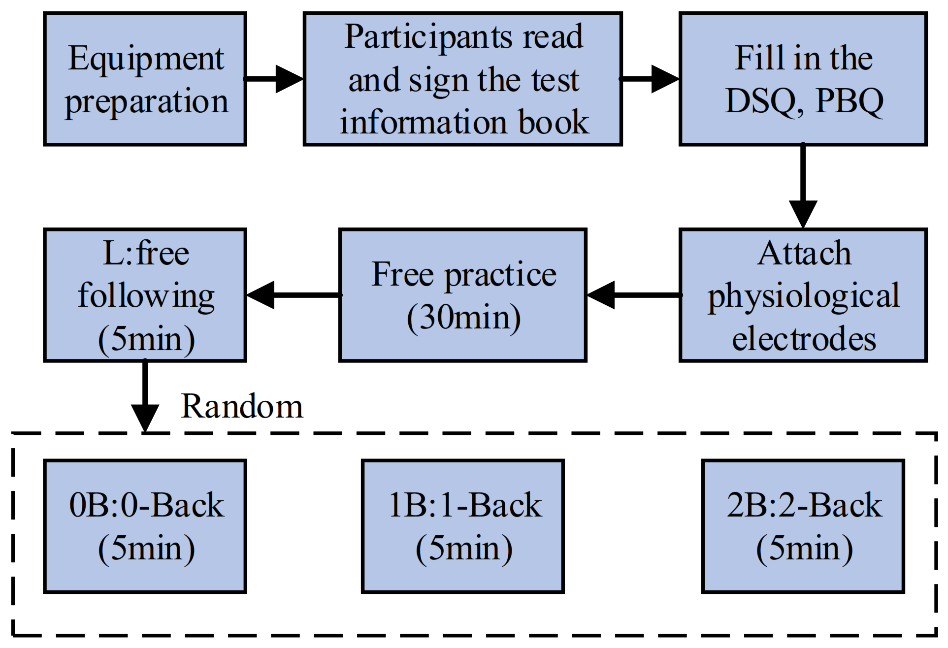
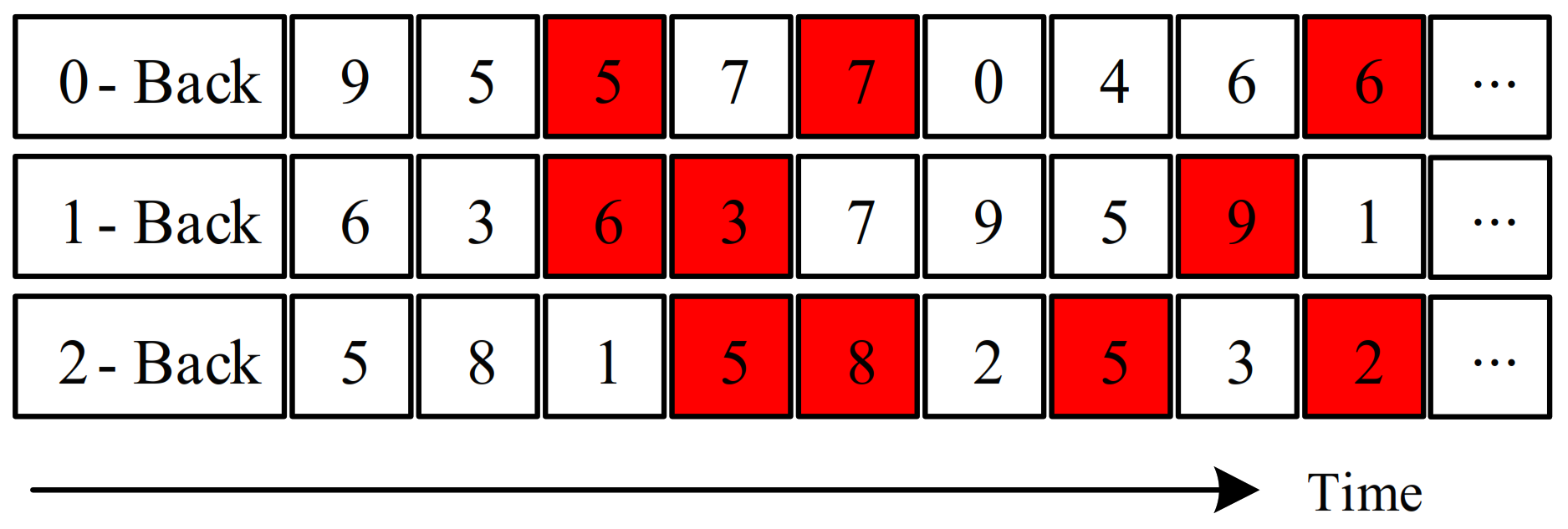
2.2. Test Procedure
2.3. Data Extraction and Pre–Processing
2.4. Data Fundamental Analysis
2.4.1. Subjective Data Analysis
2.4.2. Variable Threshold Definition
3. Methods
3.1. Description of the Driving Process Based on HSMM
3.1.1. Construction of HDP–HSMM
3.1.2. Parameter Sampling and Inference
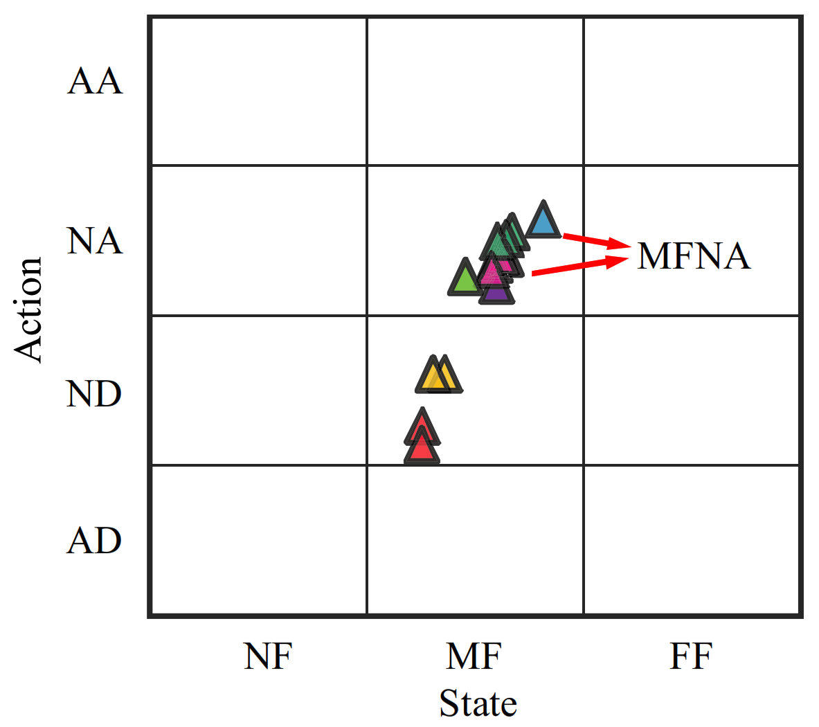
3.2. Construction of the State–Action Semantic Plane
3.3. Quantification of the Driving Style Method
4. Results
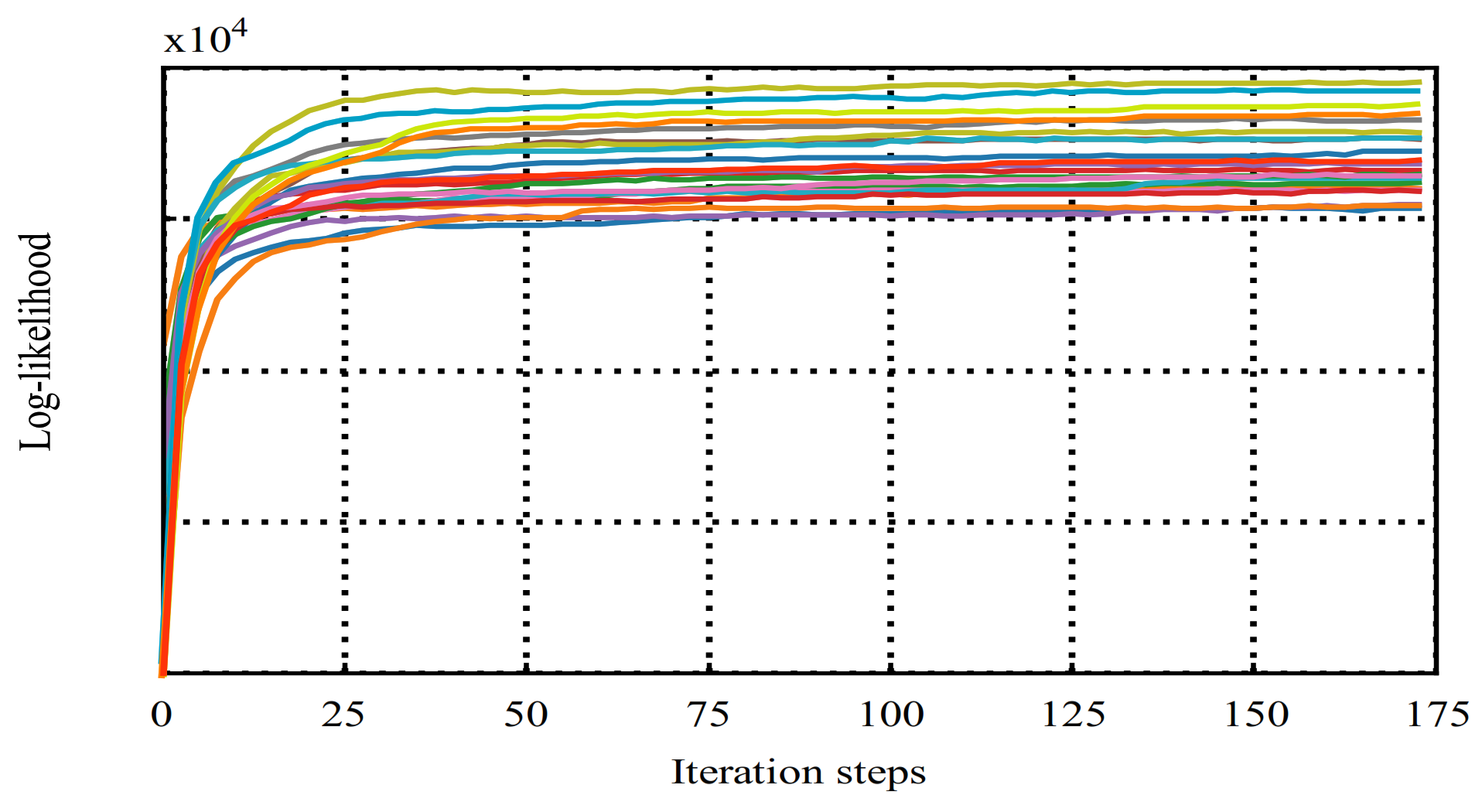
4.1. Model Training Results
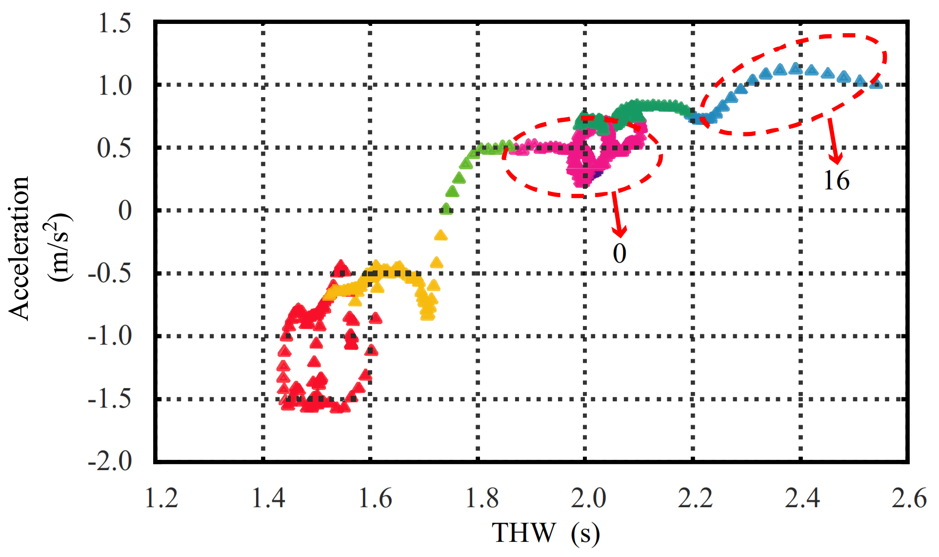
4.2. Driving Data Fragment Results
4.3. Fragment Sequence Cluster Labelling Results
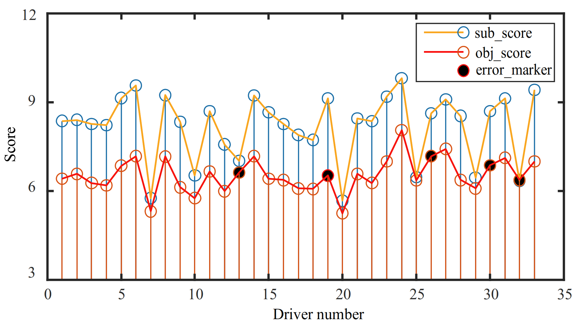
4.4. Correlation Analysis of the Subjective Score and Objective Risk Score
5. Discussion
5.1. Driving Style Discussion
5.1.1. Frequency and Duration Proportion of Driving Behavior
5.1.2. The Transition Probabilities of Driving Behavior
5.2. Application of Transition Probabilities
6. Conclusions
- (1)
- The HDP–HSMM algorithm combines the advantages of infinite clustering and adaptive updating in the HDP algorithm with the description of the dynamic random process in HSMM. It can decompose time series driving data into the fragment clusters with similar characteristics. This algorithm can be further used for the characteristic extraction of a large amount of naturistic driving data.
- (2)
- The driving behavior semantic plane was developed. It can interpret the fragment clusters, quantify the drivers’ risk indices by determining the probability and duration proportion of each behavior, and intuitively express the driving preferences of drivers with different styles. The aggressive drivers prefer NFNA and NFNA, high–risk driving behaviors, in which probability frequency reaches 79.7% and the duration proportion reaches 75.4%. The cautious drivers prefer low–risk driving behaviors, such as FFNA and FFND, with a probability of 66.67% and a duration proportion of 61.04%.
- (3)
- Additionally, the action behavior of aggressive acceleration (AA) and aggressive deceleration (AD) is lower under highway conditions, which is consistent with the actual situation.
- (4)
- Transition probability can reveal the internal relationship among driving behaviors. The joint mutual information maximization (JMIM) algorithm can select an optimized subset effectively by combining feature correlation and redundancy concepts. The seven highest ranking features were selected to evaluate driving styles: (1) MFND–MFNA, (2) NFAD–NFND, (3) NFND–NFNA. (4) NFND–NFAD, (5) FFND–FFNA, (6) MFND–FFNA, and (7) FFNA–FFND. The results showed that the transition probability as classification features can provide rich information about driving style and improve the classification accuracy of the driving style.
Author Contributions
Funding
Institutional Review Board Statement
Informed Consent Statement
Acknowledgments
Conflicts of Interest
References
- Li, M.; Song, X.; Cao, H.; Wang, J.; Huang, Y.; Hu, C.; Wang, H. Shared Control with a Novel Dynamic Authority Allocation Strategy Based on Game theory and Driving Safety Field. Mech. Syst. Signal Process. 2019, 124, 199–216. [Google Scholar] [CrossRef]
- Itkonen, T.; Lehtonen, E.; Selpi, S. Characterisation of Motorway Driving Style Using Naturalistic Driving Data. Transp. Res. Part F Traffic Psychol. Behav. 2020, 69, 72–79. [Google Scholar] [CrossRef]
- Cao, H.; Zhao, S.; Song, X.; Bao, S.; Li, M.; Huang, Z.; Hu, C. An optimal hierarchical framework of the trajectory following by convex optimisation for highly automated driving vehicles. Veh. Syst. Dyn. 2019, 57, 1287–1317. [Google Scholar] [CrossRef]
- Martinez, C.; Heucke, M.; Wang, F.; Gao, B.; Cao, D. Driving Style Recognition for Intelligent Vehicle Control and Advanced Driver Assistance: A Survey. IEEE Trans Intell. Transp. Syst. 2020, 2018, 666–676. [Google Scholar] [CrossRef] [Green Version]
- Moller, M.; Haustein, S. Keep on Cruising: Changes in Lifestyle and Driving Style Among Male Drivers Between the Age of 18 and 23. Transp. Res. Part F Psychol. Behav. 2013, 20, 59–69. [Google Scholar] [CrossRef]
- Zhu, B.; Jiang, Y.; Zhao, J.; He, R.; Bian, N.; Deng, W. Typical-driving-style-oriented Personalized Adaptive Cruise Control Design Based on Human Driving Data. Transp. Res. Part C Emerg. Technol. 2019, 100, 274–288. [Google Scholar] [CrossRef]
- Yang, W.; Zheng, L.; Li, Y.; Ren, Y.; Zhou, X. Automated Highway Driving Decision Considering Driver Characteristics. IEEE Trans. Intell. Transp. Syst. 2020, 21, 2350–2359. [Google Scholar] [CrossRef]
- Li, G.; Li, S.E.; Cheng, B.; Green, P. Estimation of Driving Style in Naturalistic Highway Traffic Using Maneuver Transition Probabilities. Transp. Res. Part C Emerg. Technol. 2017, 74, 113–125. [Google Scholar] [CrossRef]
- Toledo, T.; Musicant, O.; Lotan, T. In-Vehicle Data Recorders for Monitoring and Feedback on Drivers’ Behavior. Transp. Res. Part C Emerg. Technol. 2008, 16, 320–331. [Google Scholar] [CrossRef]
- Ma, Y.; Fu, R. Research and Development of Drivers Visual Behavior and Driving Safety. China J. Highw. Transp. 2015, 28, 82–94. [Google Scholar]
- Bazzan, A.; Klugl, F. A Review on Agent-Based Technology for Traffic and Transportation. Knowl. Eng. Rev. 2014, 29, 375–403. [Google Scholar] [CrossRef]
- Ehsani, J.; Li, K.; Simons, B.; Mcgrath, C.; Perlus, J.; O’Brien, F.; Klauer, S. Conscientious Personality and Young Drivers’ Crash Risk. J. Saf. Res. 2015, 54, 83.e29–87.e29. [Google Scholar] [CrossRef] [PubMed] [Green Version]
- Bellem, H.; Schoenenberg, T.; Krems, J.; Schrauf, M. Objective Metrics of Comfort: Developing A Driving Style for Highly Automated Vehicles. Transp. Res. Part F Traffic Psychol. Behav. 2016, 41 Pt A, 45–54. [Google Scholar] [CrossRef]
- Schockenhoff, F.; Nehse, H.; Lienkamp, M. Maneuver-Based Objectification of User Comfort Affecting Aspects of Driving Style of Autonomous Vehicle Concepts. Appl. Sci. 2020, 10, 3946. [Google Scholar] [CrossRef]
- Schwarzer, V.; Ghorbani, R. Drive Cycle Generation for Design Optimization of Electric Vehicles. IEEE Trans. Veh. Technol. 2012, 62, 89–97. [Google Scholar] [CrossRef]
- Higgs, B.; Abbas, M. Segmentation and Clustering of Car-Following Behavior: Recognition of Driving Patterns. IEEE Trans. Intell. Transp. Syst. 2014, 16, 81–90. [Google Scholar] [CrossRef]
- Zhringer, M.; Kalt, S.; Lienkamp, M. Compressed Driving Cycles Using Markov Chains for Vehicle Powertrain Design. World Electr. Veh. J. 2020, 11, 52. [Google Scholar] [CrossRef]
- Taniguchi, T.; Nagasaka, S.; Hitomi, K.; Takenaka, K.; Bando, T. Unsupervised Hierarchical Modeling of Driving Behavior and Prediction of Contextual Changing Points. IEEE Trans. Intell. Transp. Syst. 2015, 16, 1746–1760. [Google Scholar] [CrossRef]
- Taniguchi, T.; Nagasaka, S.; Hitomi, K.; Chandrasiri, N.; Bando, T.; Takenaka, K. Sequence Prediction of Driving Behavior Using Double Articulation Analyzer. IEEE Trans. Syst. Man Cybern. Syst. 2016, 46, 1300–1313. [Google Scholar] [CrossRef]
- Lim, H.; Choi, H.; Choi, Y.; Kim, I.-J. Memetic algorithm for multivariate time-series segmentation. Pattern Recognit. Lett. 2020, 138, 60–67. [Google Scholar] [CrossRef]
- Bargi, A.; Xu, R.; Piccardi, M. An Adaptive Online HDP-HMM for Segmentation and Classification of Sequential Data. IEEE Trans. Neural Netw. Learn. Syst. 2018, 29, 3953–3968. [Google Scholar] [CrossRef] [PubMed]
- Xu, L.; Hu, J.; Jiang, H.; Meng, W. Establishing Style-Oriented Driver Models by Imitating Human Driving Behaviors. IEEE Trans. Intell. Transp. Syst. 2015, 16, 2522–2530. [Google Scholar] [CrossRef]
- Tadesse, E.; Sheng, W.; Liu, M. Driver drowsiness detection through HMM based dynamic modelling. In Proceedings of the IEEE International Conference on Robotics and Automation (ICRA), Hong Kong, China, 31 May–7 June 2014; pp. 4003–4008. [Google Scholar]
- Gadepally, V.; Krishnamurthy, A.; Özgüner, Ü. A Framework for Estimating Driver Decisions Near Intersections. IEEE Trans. Intell. Transp. Syst. 2013, 15, 637–646. [Google Scholar] [CrossRef]
- Han, W.; Wang, W.; Li, X.; Xi, J. Statistical-based Approach for Driving Style Recognition Using Bayesian Probability with Kernel Density Estimation. IET Intell. Transp. Syst. 2018, 13, 22–30. [Google Scholar] [CrossRef] [Green Version]
- Xue, Q.; Wang, K.; Lu, J.J.; Liu, Y. Rapid Driving Style Recognition in Car-Following Using Machine Learning and Vehicle Trajectory Data. J. Adv. Transp. 2019, 2019 Pt 1, 9085238. [Google Scholar] [CrossRef] [Green Version]
- Bellem, H.; Thiel, B.; Schrauf, M.; Krems, J. Comfort in automated driving: An analysis of preferences for different automated driving styles and their dependence on personality traits. Transp. Res. Part F Traffic Psychol. Behav. 2018, 55, 90–100. [Google Scholar] [CrossRef]
- Zheng, L.; Qiao, X.; Ni, T.; Yang, W.; Li, Y. Driver Cognitive Load Based on Multi-Dimensional Information Feature Analysis. China J. Highw. Transp. 2021, 34, 240–250. [Google Scholar]
- Wong, C.; Mao, Y.; Peng, K.; Shi, J. Differences between odd number and even number response formats: Evidence from mainland Chinese respondents. Asia Pac. J. Manag. 2011, 28, 379–399. [Google Scholar] [CrossRef]
- Kondoh, T.; Yamamura, T.; Kitazaki, S.; Kuge, N.; Boer, E.R. Identification of Visual Cues and Quantification of Drivers’ Perception of Proximity Risk to the Lead Vehicle in Car-Following Situations. J. Mech. Syst. Transp. Logist. 2008, 1, 170–180. [Google Scholar] [CrossRef] [Green Version]
- Nilsson, J.; Falcone, P.; Vinter, J. Safe Transitions from Automated to Manual Driving Using Driver Controllability Estimation. IEEE Trans. Intell. Transp. Syst. 2015, 16, 1806–1816. [Google Scholar] [CrossRef]
- Kusano, K.D.; Chen, R.; Montgomery, J.; Gabler, H.C. Population Distributions of Time to Collision at Brake Application During Car Following from Naturalistic Driving Data. J. Saf. Res. 2015, 54, 95.e29–104.e29. [Google Scholar] [CrossRef] [PubMed]
- Wang, W.; Zhao, D.; Xi, J.; Han, W. A Learning-Based Approach for Lane Departure Warning Systems with A Personalized Driver Model. IEEE Trans. Veh. Technol. 2018, 67, 9145–9157. [Google Scholar] [CrossRef] [Green Version]
- Zhou, J.; Wang, F.; Zeng, D. Hierarchical Dirichlet Processes and Their Applications: A Survey. Acta Autom. Sin. 2011, 4, 389–407. [Google Scholar] [CrossRef]
- Wang, W.; Xi, J.; Ding, Z. Driving Style Analysis Using Primitive Driving Patterns with Bayesian Nonparametric Approaches. IEEE Trans. Intell. Transp. Syst. 2018, 20, 2986–2998. [Google Scholar] [CrossRef] [Green Version]
- The, Y.W.; Jordan, M.I.; Beal, M.J.; Blei, D.M. Hierarchical Dirichlet Processes. J. Am. Stat. Assoc. 2006, 101, 1566–1581. [Google Scholar]
- Sethurman, J. A Constructive Definition of Dirichlet Priors. Stat. Sin. 1994, 4, 639–650. [Google Scholar]
- Johnson, M.; Willsky, A. The Hierarchical Dirichlet Process Hidden Semi-Markov Model. In Proceedings of the Twenty-Sixth Conference on Uncertainty in Artificial Intelligence (UAI2010), Catalina Island, CA, USA, 8–11 July 2010; Association for Uncertainty in Artificial Intelligence: Catalina Island, CA, USA, 2012; pp. 252–259. [Google Scholar]
- Fox, E. Bayesian Nonparametric Learning of Complex Dynamical Phenomena. Ph.D. Thesis, MIT, Cambridge, MA, USA, 2009. [Google Scholar]
- Bennasar, M.; Hicks, Y.; Setchi, R. Feature Selection Using Joint Mutual Information Maximisation. Expert Syst. Appl. 2015, 42, 8520–8532. [Google Scholar] [CrossRef] [Green Version]
- Gao, B.; Cai, K.; Qu, T.; Hu, Y.; Chen, H. Personalized Adaptive Cruise Control Based on Online Driving Style Recognition Technology and Model Predictive Control. IEEE Trans. Veh. Technol. 2020, 69, 12482–12496. [Google Scholar] [CrossRef]


| Types of Data | Information |
|---|---|
| driver operation | brake/accelerator pedal position, turn signal, steering angle |
| ego vehicle states | speed, acceleration, location information, yaw angle speed, engine speed |
| preceding vehicle states | speed, acceleration, location information |
| subjective score | DSQ, RPQ |
| physiological signal | ECG, GSR, EEG |
| Driving Styles | Sample Number | Cluster Center |
|---|---|---|
| Cautious | 7 | 6.49 |
| Normal | 16 | 8.42 |
| Aggressive | 10 | 9.30 |
| Variables | States/Actions | Thresholds |
|---|---|---|
| THW (s) | near following (NF) | <1.2 |
| middle following (MF) | [1.2,3.0] | |
| far following (FF) | >3.0 | |
| Acceleration (m/s2) | aggressive acceleration (AA) | >1.6 |
| normal acceleration (NA) | [0,1.6] | |
| normal deceleration (ND) | [−1.4,0] | |
| aggressive deceleration (AD) | <−1.4 |
| Score Transition | Behavior Transition | Aggressive | Normal | Cautious | Significance Level | |||
|---|---|---|---|---|---|---|---|---|
| Mean | Std | Mean | Std | Mean | Std | p | ||
| 6–7 | MFND–MFNA | 0.6281 | 0.1917 | 0.6453 | 0.1395 | 0.2787 | 0.2346 | 0 < 0.05 |
| 7–8 | NFAD–NFND | 0.7382 | 0.3201 | 0.4494 | 0.2271 | 0.0444 | 0.1721 | 0 < 0.05 |
| 7–9 | NFAD–NFNA | 0.4408 | 0.2353 | 0.3369 | 0.2812 | 0.1111 | 0.2999 | 0.0016 < 0.05 |
| 8–7 | NFND–NFAD | 0.2492 | 0.1625 | 0.1119 | 0.1396 | 0 | 0 | 0 < 0.05 |
| 4–5 | FFND–FFNA | 0.3347 | 0.3499 | 0.5005 | 0.2803 | 0.8106 | 0.0941 | 0 < 0.05 |
| 5–4 | FFNA–FFND | 0.3871 | 0.2168 | 0.5751 | 0.2287 | 0.7363 | 0.1842 | 0 < 0.05 |
| 7–8 | MFNA–NFND | 0.1051 | 0.0873 | 0.0575 | 0.0581 | 0.0321 | 0.0649 | 0.0021 < 0.05 |
| Input Features | Classifiers | Aggressive | Normal | Cautious |
|---|---|---|---|---|
| Transition probability | RF | 91.35% | 87.26% | 92.22% |
| SVM | 83.53% | 81.64% | 84.91% | |
| KNN | 88.92% | 84.43% | 87.43% | |
| Statistical features | RF | 88.49% | 83.26% | 86.32% |
| SVM | 84.46% | 79.27% | 82.08% | |
| KNN | 88.13% | 82.64% | 82.40% |
| Correlation | MFND–MFNA | NFAD–NFND | NFAD–NFNA | NFND–NFAD | FFND–FFNA | FFNA–FFND | MFNA–NFND |
|---|---|---|---|---|---|---|---|
| MFND–MFNA | 1 | 0.1494 | 0.0687 | 0.0679 | −0.2143 | −0.1598 | 0.0857 |
| NFAD–NFND | 0.1494 | 1 | 0.5621 | 0.6491 | −0.4193 | −0.4520 | 0.4578 |
| NFAD–NFNA | 0.0687 | 0.5621 | 1 | 0.2014 | −0.2554 | −0.1145 | 0.6391 |
| NFND–NFAD | 0.0679 | 0.6491 | 0.2014 | 1 | −0.2336 | −0.3098 | 0.3264 |
| FFND–FFNA | −0.2143 | −0.4193 | −0.2554 | −0.2336 | 1 | 0.5029 | −0.1657 |
| FFNA–FFND | −0.1598 | −0.4520 | −0.1145 | −0.3098 | 0.5029 | 1 | −0.1336 |
| MFNA–NFND | 0.0857 | 0.4578 | 0.6391 | 0.3264 | −0.1657 | −0.1336 | 1 |
| Correlation | Ve_mean | Ve_std | De_mean | De_std | Ae_mean | Ae_std | THW_mean |
|---|---|---|---|---|---|---|---|
| Ve_mean | 1 | 0.6025 | −0.5068 | −0.3547 | 0.1605 | 0.3657 | −0.6764 |
| Ve_std | 0.6025 | 1 | −0.2731 | −0.2084 | 0.0464 | 0.4818 | −0.3277 |
| De_mean | −0.5068 | −0.2731 | 1 | 0.8666 | −0.0749 | −0.4843 | 0.9674 |
| De_std | −0.3547 | −0.2084 | 0.8666 | 1 | 0.1078 | −0.4450 | 0.8225 |
| Ae_mean | 0.1605 | 0.0464 | −0.0749 | 0.1078 | 1 | −0.0480 | −0.1429 |
| Ae_std | 0.3657 | 0.4818 | −0.4843 | −0.4450 | −0.0480 | 1 | −0.4115 |
| THW_mean | −0.6764 | −0.3277 | 0.9674 | 0.8225 | −0.1429 | −0.4115 | 1 |
Publisher’s Note: MDPI stays neutral with regard to jurisdictional claims in published maps and institutional affiliations. |
© 2021 by the authors. Licensee MDPI, Basel, Switzerland. This article is an open access article distributed under the terms and conditions of the Creative Commons Attribution (CC BY) license (https://creativecommons.org/licenses/by/4.0/).
Share and Cite
Qiao, X.; Zheng, L.; Li, Y.; Ren, Y.; Zhang, Z.; Zhang, Z.; Qiu, L. Characterization of the Driving Style by State–Action Semantic Plane Based on the Bayesian Nonparametric Approach. Appl. Sci. 2021, 11, 7857. https://doi.org/10.3390/app11177857
Qiao X, Zheng L, Li Y, Ren Y, Zhang Z, Zhang Z, Qiu L. Characterization of the Driving Style by State–Action Semantic Plane Based on the Bayesian Nonparametric Approach. Applied Sciences. 2021; 11(17):7857. https://doi.org/10.3390/app11177857
Chicago/Turabian StyleQiao, Xuqiang, Ling Zheng, Yinong Li, Yuqing Ren, Zhida Zhang, Ziwei Zhang, and Lihong Qiu. 2021. "Characterization of the Driving Style by State–Action Semantic Plane Based on the Bayesian Nonparametric Approach" Applied Sciences 11, no. 17: 7857. https://doi.org/10.3390/app11177857
APA StyleQiao, X., Zheng, L., Li, Y., Ren, Y., Zhang, Z., Zhang, Z., & Qiu, L. (2021). Characterization of the Driving Style by State–Action Semantic Plane Based on the Bayesian Nonparametric Approach. Applied Sciences, 11(17), 7857. https://doi.org/10.3390/app11177857