Advanced Trajectory Control for Piezoelectric Actuators Based on Robust Control Combined with Artificial Neural Networks

Abstract

In applications where high precision in micro- and nanopositioning is required, piezoelectric actuators (PEA) are an optimal micromechatronic choice. However, the accuracy of these devices is affected by a natural phenomenon called “hysteresis” that even increases the instability of the system. This anomaly can be counteracted through a material re-shape or by the design of a control strategy. Through this research, a novel control design has been developed; the structure contemplates an artificial neural network (ANN) feedforward to contract the non-linearities and a robust close-loop compensator to reduce the unmodelled dynamics, uncertainties and perturbations. The proposed scheme was embedded in a dSpace control platform with a Thorlabs PEA; the parameters were tuned online through specific metrics. The outcomes were compared with a conventional proportional-integral-derivative (PID) controller in terms of control signal and tracking performance. The experimental gathered results showed that the advanced proposed strategy had a superior accuracy and chattering reduction.

1. Introduction

A piezoelectric actuator (PEA) is a device that transduces an applied voltage into a mechanical displacement that can be in the order of nano- and micrometers. This is a huge advantage for several applications where precision is needed. For instance, optical microsurgery requires displacement capabilities from a surgeon that can be complex to achieve since the precision needed is around 10 $\mathsf{\mu }$m [1]. An additional example is the employment of PEAs in motors where not only proper accuracy is required but also the stiffness of the actuator is a critical feature, which is another main advantage of piezoelectric actuators [2].

Regardless the benefits of PEAs, which are extensive for several uses, downsides have significant importance in the performance of these appliances. One of the main and most studied ones is hysteresis, which is a ferroelectric phenomenon related to the material poles that have arbitrary orientations that align when a voltage is applied, but the release of this action yields to a different direction [3,4]. Thus, for this reason, it is also known as a memory effect as it depends on previous history [5]. In practice, the accuracy can be reduced by up to 22% of the nominal displacement as a consequence of this anomaly [6]; another important consequence of this phenomenon is also the instability [7]. Nevertheless, since hysteresis is a natural property, available solutions comprise a material re-design or the implementation of a control algorithm [4].

Proportional-integral-derivative (PID) had been widely used in practice as a first option. Authors of [8] developed a PID for the position, which was verified in simulations and later in experiments where the results showed a tracking error reduction of 5%. A main disadvantage of PIDs is the gain scheduling, which can vary for different scenarios and or situations; thus, several ways have been suggested to tune these. For instance, the authors of [9] proposed the usage of particle swarm optimisation (PSO) in a simulation with a suitable PEA model. The obtained gains were used in an experimental platform with a commercial PEA where the results showed an improvement in the position accuracy. However, online tuning algorithms for experimental rigs can require a significant amount of computational resources, and certainly, there are other non-linear controllers that manage the compensation with better performance.

Sliding mode control (SMC) is a non-linear strategy with a discontinuity that drives the system in a sliding surface [10]. The main advantage is the robustness against uncertainties and external disturbances. The classic SMC has been implemented in PEAs for force control by the authors of [11], where they found suitable outcomes with sine signals as references. A similar approach was carried out in the research of Chouza et al. [12], where SMC based with a PID surface was implemented in a commercial PEA where they tested different reference signals, such as the ramp, constants and sine wave. In spite of the improvements of error reduction in the ramp and constant references, the sine wave showed an error of around 5%. However, in the analysed background, it was shown that the main disadvantage of SMC is the chattering that is generated by the discontinuous property. This is an unwanted effect because it increases the energy loss and also the wear in the actuator [13].

Certainly, the chattering can only be reduced and not eliminated because the discontinuity (produced by a sign function) is on of the main features of SMC. Thus, in the recent years, many proposals have been published to trim this effect. For instance, the authors of [14] changed the discontinuity by a hyperbolic function, and in comparison with conventional approaches, the enhancement was acknowledged in the results. Another advance strategy is the usage of high order sliding mode controllers (HOSMC), where high order derivatives are used in the sliding surface, and as a result, the chattering is relieved [15,16]. An example of implementation has been carried out by the authors of [17], where they used an HOSMC as an observer for error compensation in a PEA test rig. The results showed significant improvements in comparison with other conventional types of SMC strategies in simulation and experiments. Regardless of the enhancement of HOSMC over conventional SMC, the design of sliding controllers establishes that the control law is split into a switching and an equivalent term that are aimed to maintain and compensate the sliding motion [18]. The equivalent is commonly achieved through a mathematical model that describes the system, and this would imply the use of a proper hysteresis description.

Hysteresis models for PEAs are mainly classified in two main categories: physical and phenomenological [19]. The first-mentioned group is a description of the ferromagnetic effect that produces the non-linearity, although the material dependency and complex numerical solutions are the downsides of these theories [20,21]. In regards to the phenomenological, the sub-classification is related to the ones based on differential equations (Dunhem [22], Backslash [23] and Bouc-Wen [24]), operator models (Preisach [5], Prandtl-Ishlinskii [25] and Krasnoselskii-Pokrovskii [26]) and polynomial models [27]. Nevertheless, the disadvantages of these approaches are linked with complicated solutions to gather the inverse model, incapability to deal with asymmetric hysteresis, rate dependency and complex implementation [20].

Based on the research about the background that we made, we designed an HOSMC controller known as QC-Continuous (QCSMC), which provides suitable results in terms of chattering reduction in previous works [28]. Due to the drawbacks that we enumerated about hysteresis models, we decided to achieve the equivalent term of the sliding controller through means of an artificial neural network (ANN). This is possible because we could conduct experiments to acquire data for the ANN training.

The structure of this article is arranged as follows. In Section 2, we provided a description about the hardware employed for the experiments within their technical specifications, a hysteresis explanation of the PEA used, and the controllers designed within the metrics used to contrast their performance. Section 3 provides the obtained results of the trained ANN and the control implementation outcomes. Finally, in Section 4, we recap the most important features obtained within the research.

2. Materials Furthermore, Methods

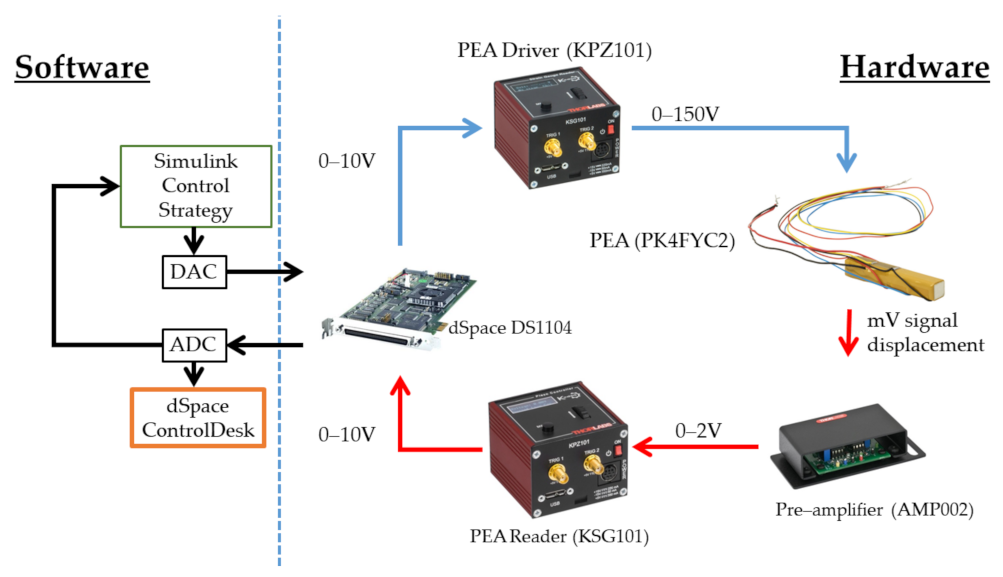
2.1. Hardware Description

The main hardware that we used is a Thorlabs PK4FYC2 PEA that was produced with several piezoelectric chips wedged with epoxy and glass beads. A maximum displacement of 38.5 $\mathsf{\mu }$m is achieved with a driving voltage of 150 V. As the device is frequently handled for precise and micrometric displacement, the manufacturer included four strain gauges arrayed in a Wheatstone bridge so that the measurement could be obtained from resistance variation, which provides a better resolution [29].

The PEA accessories include a driver cube KPZ101, whose input signal is 0–10 V and is transformed into a 0–150 V to manage the PEA. As the PEA delivers an output voltage that is in the order of milivolts, a pre-amplifier augments this value into a 0–2 V signal. The latter is transferred into a reader cube KSG101, which transforms the voltage into 0–10 V. Further technical details of the PEA and its peripherals are summarized in

Table 1. Thorlabs hardware used.

PEA PK4FYC2	Values	Units
Maximum displacement	38.5	$\mathsf{\mu }$m
Blocking force	1000	N
Resonant frequency	34	kHz
Maximum error	15	%
Driver Cube KPZ101
Output driving voltage for PEA	150	V
Input driving voltage	0–10	V
Maximum output bandwidth	1	kHz
Reader Cube KSG101
Output range	0–10	V
Resolution	1	nm
Pre-Amplifier AMP002
Output range	0–2	V

.

Since the input and output signals of the PEA are in the range of 0–10 V, we, therefore, used a proper platform for acquisition and control, such as the dSpace DS1104 board. We linked this device to a Dell Precision Workstation T3500 through a peripheral component interconnect (PCI) for monitoring and control. Moreover, the DS1104 has an external connector panel CP1104 that we connected to the PEA driver and reader.

In regards to the software, we developed the proposed strutures in Simulink by Mathworks and embedded them through the platform dSpace real-time interface (RTI). This allowed us to generate and manage a real-time control algorithm, while the RTI helped to reduce the compilation time. All the information was acquired with ControlDesk and processed with MATLAB by Mathworks. The explained relation between software and hardware is detailed in Figure 1. The chosen sampling time was 1kHz as it is a suitable match with the acquisition and the hardware physical limits.

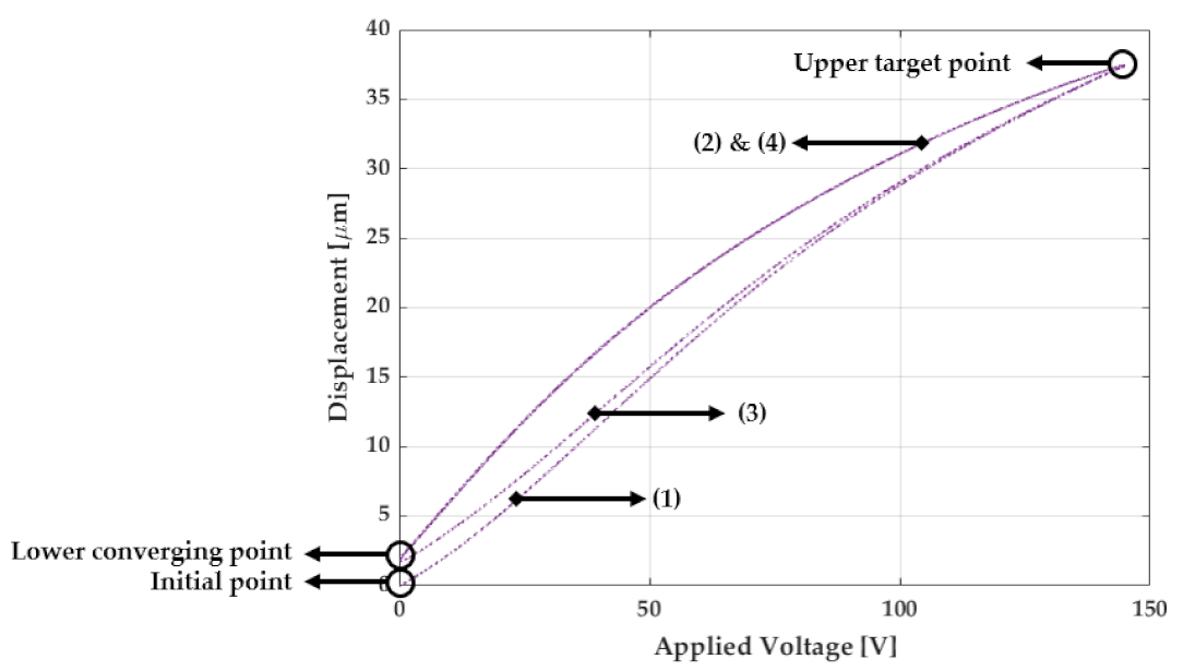
2.2. Hysteresis Description and Reference Design

Common excitation signals that represent a suitable hysteresis graph in PEAs are triangular and sine waves [5]. The triangular waveform is a complex input for the PEA, as it not only implies that sharp slope changes are required to be followed, but also this wave is generated from high-frequency harmonics [30]. Therefore, we developed a triangular reference of a 145V amplitude, which is lower than the maximum allowed voltage so that the PEA lifetime is not affected; additionally, we chose a period of 4 s for this signal.

With the previously described triangular waveform as an output, we acquired the displacement of the PEA where the outcome is the one shown in Figure 2. The mechanics and features of the curve are developed as follows from the beginning of the applied voltage:

• Initial point: We calibrated the PEA so that it initially starts at a zero displacement from this.
• Curve (1): This is known as the initial ascending curve, which begins from the previously described point and ends at the upper target point. As the figure shows, the non-linearity is present along this path.
• Upper target point: At this place, the PEA reached the correspondent displacement to the specified amplitude of the triangular waveform.
• Curve (2): This, known as the second ascending curve, shows that the PEA has an asymmetric hysteresis, which is a phenomenon that creates difficulties when mathematical models need to be found to reflex.
• Lower converging point: Ideally, the final position could have been at the initial point when the applied voltage is null. However, in this case, the lower converging point is not the same as the initial point.
• Curve (3): Provided that amplitude and period are the same along the experiment, then this curve will be equal for the following ascending cycles.
• Curve (4): As with the curve (3), this course will be the same provided that the reference configuration is constant.

Taking into account the previous analysis, we designed the reference considering the applied voltage in the PEA. As a first consideration, the initial point within the first ascending curve is negligible to evaluate the performance of the PEA in a long-term experiment. Therefore, we outlined a reference between the lower converging and upper target point as linear Equation (1) reflects. In this mathematical expression, we defined X as the displacement, $\alpha$ the slope between the two points of interests and b the vertical offset in terms of the lower converging point.

$$X\left[\mathsf{\mu }\mathrm{m}\right]=\alpha ·V+b$$

(1)

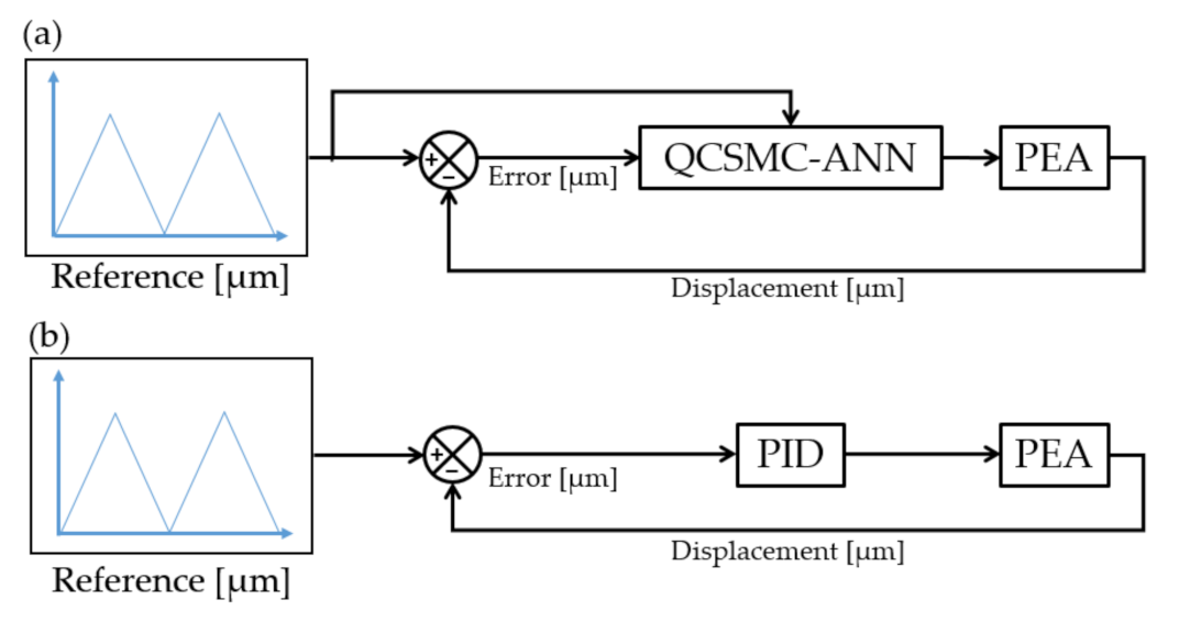
2.3. Contrasted Schemes and Their Design

Based on the framework that we proposed, we decided to contrast it with a PID controller, a commonly used structure in the industry and PEA tracking performance. A simplified description of the used controllers is displayed in Figure 3. We designed the structure by taking into account the advantages of the RTI properties so that the variables of each controller could be changed in real-time. We developed the quest to find these values through the online minimization of the integral of the absolute error (IAE). Equation (2) express the IAE, where $e_i$ is the error in at the i-th sample, $\mathrm{\Delta }$t is the sampling time and N the number of points chosen to calculate the value.

$$IAE=\sum _{i=1}^N\left|e_i\right|\mathrm{\Delta }t$$

(2)

Another statistical metric used is the root-mean-square-error (RMSE), which reflects the precision of each framework in terms of the error. Equation (3) is the mathematical expression of the latter-described metric.

$$RMSE=\sqrt{{\displaystyle \frac{1}{N}}\sum _{i=1}^N{\left(e_i\right)}^2}$$

(3)

According to Ventura and Fridman [31], the chattering can be measured with Equation (4) in terms of the energy that is being dissipated from a nominal state $\overline{u}\left(t\right)$ of a control signal $u\left(t\right)$.

$$chatt\left(u\right)={\left[{\int }_{t_0}^T{\left(\dot{u}\left(t\right)-\dot{\overline{u}}\left(t\right)\right)}^{2}dt\right]}^{\frac{1}{2}}$$

(4)

2.4. Quasi-Continuous Sliding Mode Control

QC-SMC belongs to the HOSMC, known for the robustness and performance in tracking precision; moreover, the chattering reduction is another advantage of this controller over other structures [32]. The control law that we settled as Equation (5) comprises of the terms $u_{ann}$ and $u_{sw}0$, which, respectively, aim to compensate the non-linearities (such as the hysteresis) and counteract uncertainties or perturbations The definition of $u_{sw}$ is defined in Equation (6), which is dependant on a sliding surface expressed by Equation (7) and where parameters $\lambda$ and $\gamma$ are positively defined by the designer. The term $u_{ann}$ is dependant on the ANN compensation, and further details are given in the following section.

$$u=u_{ann}+u_{sw}$$

(5)

$$u_{sw}=-\gamma \frac{\dot{s}+{\left|s\right|}^{1/2}sign\left(\dot{s}\right)}{|\dot{s}{|+|s|}^{1/2}}$$

(6)

$$s=e+\lambda {\int }_0^{t}edt$$

(7)

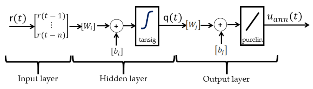
Neural Network Compensation Design

The implementation of conventional SMC methods, where the equivalent term has to be through a mathematical model, can yield to a insufficient compensation or even increase the computational cost. Nevertheless, in recent years, ANNs have been a suitable solution for system identification. The only drawback is the time that the training algorithm requires to develop a truthful output. Hence, we used a time-delay neural network (TDNN) due to the efficiency related to training time versus accuracy obtained.

In former investigations, we tested TDNN structures to reduce hysteresis, which showed proper results in combination with conventional controllers [33]. As the name states, a TDNN is an extension of a classic multilayer perceptron (MLP) that works with time signals. The inclusion of time delays n allows the neurons to get further information about the time history of the input; this implies that the ANN will fit to a time set pattern [34]. Mathematically, this is expressed with Equation (8), where f is a non-linear function that relates the input/output of the ANN. An schematic explanation is provide in Figure 4.

$$u_{ann}=f\left(x\left(t\right),x(t-1),x(t-2),\cdots ,x(t-n)\right)$$

(8)

A further expansion of the function f is as the following Equations (9)–(12): the retarded reference inputs $r(t-n)$ are weighted with parameters $W_i$ and bias $b_i$; later, this operation yields into the activation function called tansig. The output q(t), which is the outcome of the described operation, is employed as an input into the output layer. In this case, the procedure is similar as previously, but the activation is done with a linear transfer function called purelin. Subsequently, the output of this layer provides the compensation voltage $u_{ann}$.

$$q\left(t\right)=tansig\left(\sum _{p=0}^n{W}_i·r(t-n)+b_i\right)$$

(9)

$$tansig\left(x\right)=\frac{2}{1+e^{-2x}}-1.$$

(10)

$$u_{ann}=purelin[W_{j}q\left(t\right)+b_j],$$

(11)

$$purelin\left(x\right)=x.$$

(12)

The calculation of the weights and bias, related to the previous explained relations, are achieved with training algorithms. In this case, we used Levenberg–Marquardt, which represents a method that guarantees the fitting of the ANN to the experimental data through an adaptive behaviour [35]. This mechanism is generated by finding the location of the minimum of a cost function is declared as the sum of square errors and the real measurements within an iterative updating.

2.5. PID Control

The ream of PID controllers in terms of design and applications is vast, which allows a robust design even with its simple structure. Even though several tuning methods are available such as Ziegler–Nichols or Cohen–Coon [36], we used, in this case, the minimization of IAE as it was explained previously. The controller expression is the one provided in Equation (13), where $K_p$, $K_i$ and $K_d$ are, respectively, the proportional, integral and derivative gains; $\mathrm{\Delta }$t is the sampling time, and $e\left(k\right)$ is the error at a step k.

$$u\left(k\right)=K_{p}e\left(k\right)+K_i\sum _{i=1}^{k}e\left(i\right)\mathrm{\Delta }t+\frac{K_d[e\left(k\right)-e(k-1)]}{\mathrm{\Delta }t}.$$

(13)

3. Results

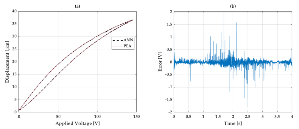
3.1. ANN Analysis Results

We recorded experimental data from the PEA where the input was a triangular signal of 145 V with a 4 s period. Furthermore, the displacement was acquired through the strain gauge reader in 40 s experiments with a sampling time of 1 kHz. From this data, we used the displacement as an input and the applied voltage as an output because the aim is to achieve an inverse model.

After several tests to achieve the best MSE, we configured the ANN in 22 neurons with 5 input delays. The data were split into 70%, 15% and 15%, respectively, for training, evaluation and testing. Finally, the performance was measured with the mean squared error (MSE) in the validation set, where the value obtained was 0.017 in 12.000 iterations made in 4 min.

Figure 5 shows the performance of the ANN to fit with the PEA hysteresis in a 4 s cycle. Although Figure 5a adapts with a decent effectiveness, Figure 5b exhibits the error where several features can be highlighted. Between 1.5 and 2.5, the error tends to increase with significant peaks; nevertheless, at 2 s, the deviation increases considerably due to the slope change as it is a complex transition to be projected by the ANN. Still, the calculated RMSE for this case provided 0.041 V in comparison to experimental data, which was acceptable.

3.2. Reference Tracking Results

The control structures were designed in Simulink, which was later embedded in the dSpace platform. Even though the main reference used was a triangle wave, we also used a sine signal (with same period and amplitude) and a variable amplitude triangular signal. The aim of this was to test the flexibility of the proposed structures against different references.

In regards to the parameters of each controller, these were reached through the minimization of the IAE in the experiments. The PID constants $K_p$, $K_i$ and $K_d$ gathered are, respectively, 1000, 10 and ${10}^{-4}$. The QCSMC-ANN parameters, $\gamma$ and $\lambda$, acquired are 60 and 8, respectively.

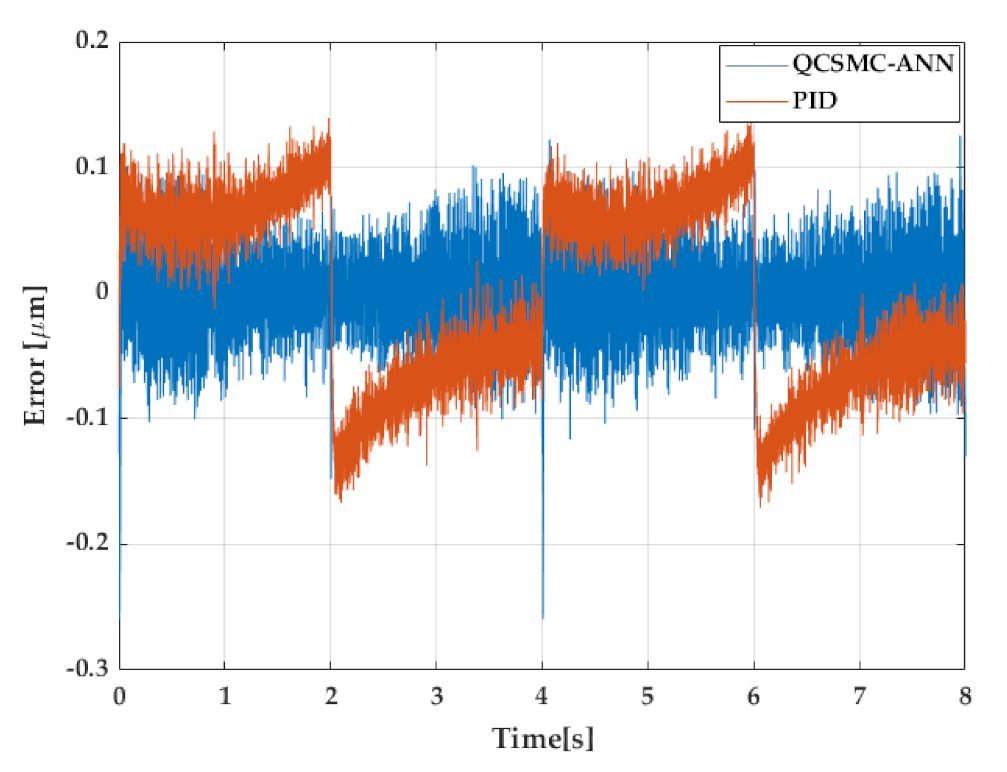
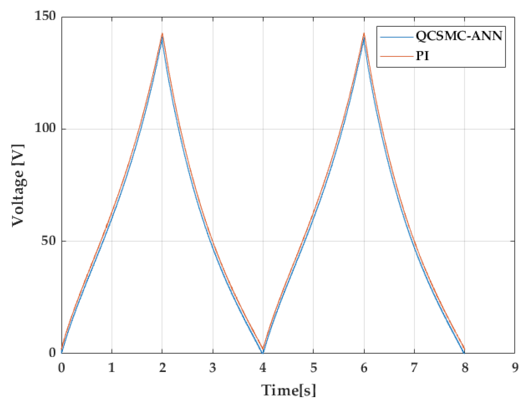
3.3. Triangular Tracking Results

The first contract was performed with a triangular wave due to its complexity to be followed. Figure 6 presents the error obtained with the QCSMC-ANN and PID in triangular cycles where several points can be highlighted. The PID controller had a variable performance since between 0 and 1 s, the error declined; however, in the following second, the error began to rise up until 2 s. Despite the QCSMC-ANN providing a high amplitude in the first second of this period, in the following, it was diminished.

Certainly, at 2 s, the first critical point appeared since it is where the slope of the triangular reference changes its sign. The PID changed suddenly from 0.1 $\mathsf{\mu }$m to near −0.12 $\mathsf{\mu }$m; although the controller performed an abrupt correction, the QCSMC-ANN generated a similar action but with a faster improvement in time. This is reflected after 2 s where the PID had transitory development without reaching the null value of the error. Nevertheless, the QCSMC-ANN carried with the same demeanour as previously right after the slope change.

The fourth second of this analysis exhibits another crucial point to focus as it is the following slope change at the lower converging point. The PID unveiled a similar situation as previously at 2 s but with lower amplitude and a subsequently transitory response. On the other hand, even if the QCSMC-ANN featured a peak that has a value above −0.2 $\mathsf{\mu }$m, the later reaction shows a similar trend as previously described, where the controller aims to a mean near the null value. After 4 s, since the signal is repeated, the detailed features are mirrored.

Aside from the error development, the control signal is an important feature to analyse because it contributes to the performance of the proposed structures. Figure 7 is a contrast of the control signal generated along the analysed error of both frameworks. As main characteristics to take into account at this point, saturations or sudden changes needed focus as these can damage the PEA driver cube. Henceforth, it can be perceived that both controllers had a suitable demeanour, and any downsides were presented in the experiments.

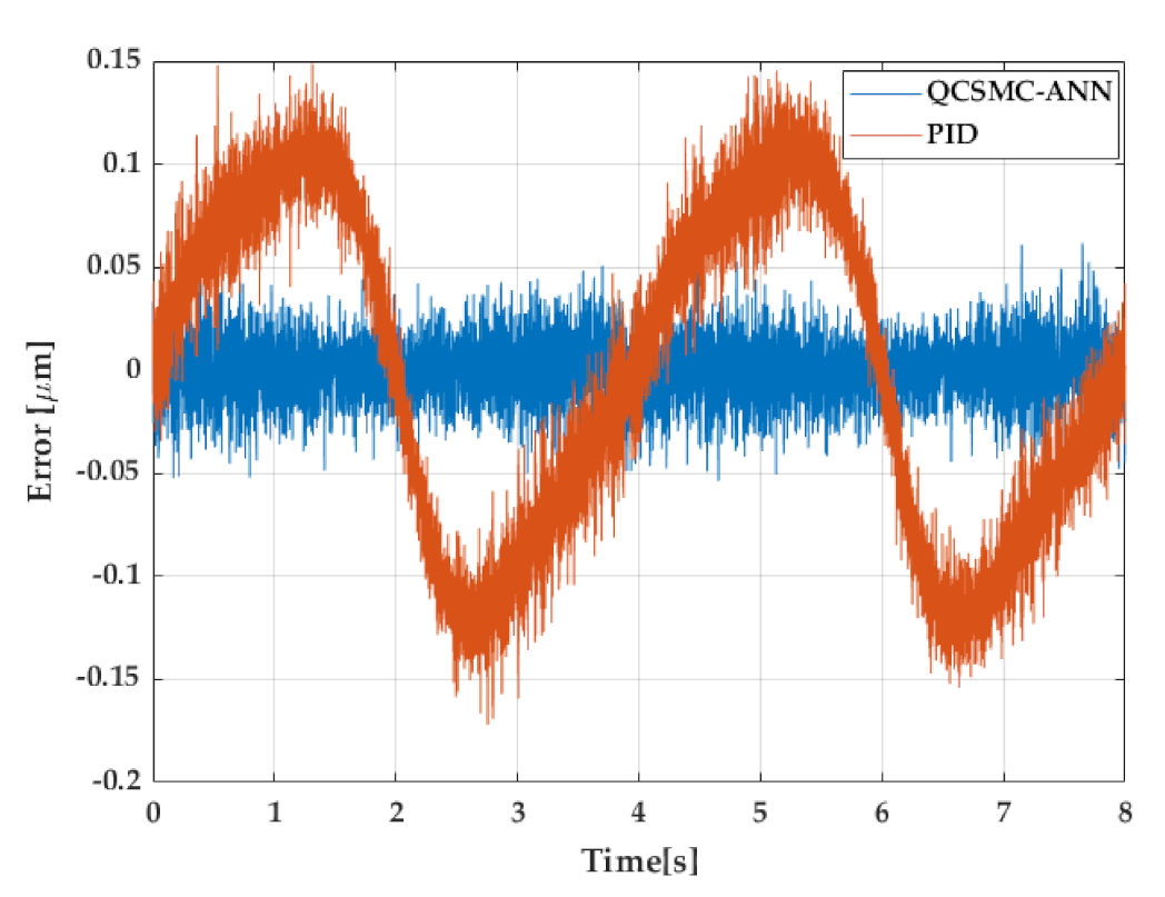
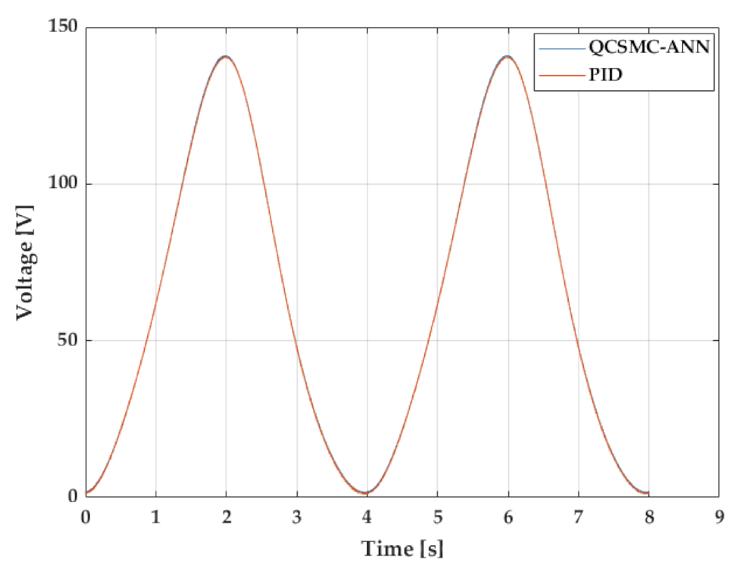
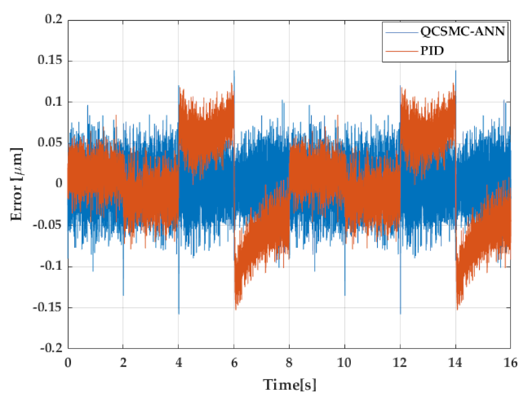
3.4. Sinusoidal Tracking Results

In pursuance of a suitable performance test that can show the docility of the proposed design against similar references, we inspected the development with a sine wave form with the same chosen amplitude and periods as previously. Figure 8 shows the error that the PID and the QCSMC-ANN produced in the mentioned reference signal. The PID had an inferior performance in relation to the previous test since after 1 s, the amplitude increased with peaks up to 0.15 $\mathsf{\mu }$m. Although the slope transition is softer in 2 s, the error kept increasing afterwards, which resulted in a variation of around 0.3 $\mathsf{\mu }$m. However, the QCSMC-ANN behaved even better than previously since the error was compensated almost equally along the test with an amplitude below 0.05 $\mathsf{\mu }$m, which oscillates around the null value.

Finally, the control signal that is presented in Figure 9 unveils a better performance than the former analysis due to the softness of the signal. It can be seen that any harm changes were developed in the analysed time, which can lead to a damage of the involved hardware.

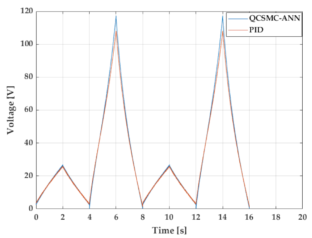
3.5. Triangular Tracking Results with Variable Amplitude

Another experiment performed is the triangular reference signal with variable amplitudes that were settled randomly in 25 V and 121 V. Figure 10 shows the repercussions of the error for the considered reference. During the first 4 s, where the amplitude was 25 V, both controllers had a similar demeanour. The PID shows a perceptible shift at the upper target point in 2 s; however, the QCSMC-ANN provided a constant development along this range with the same deviation as the PID. On the other hand, the major difference can be noticeable during 121 V, where the PID behaves similarly to previously analysed triangular signals where fast corrections occur during the slope changes of the reference signal. This effect produced a brief increment of the error amplitude in the analysed controllers, but the QCSMC-ANN managed to carry this without any transients, a feature produced by the PID.

As previously, another important feature is the control signal, which is shown in Figure 11. It can be seen that any saturations or sudden corrections that can deteriorate the hardware were developed in the performed experiments. Nevertheless, effects of chattering are analysed in further details in the following section.

3.6. Metrics Results

Certainly, for extra precise performance measurement and comparison, we used three tools that aided us to gather more conclusions. As previously explained, the IAE was used to tune the parameters until this value becomes minimum. The RMSE provides the accuracy in terms of the error, and because we implemented an SMC-based controller (known for the chattering generated in the control signal), we calculated this value based on the previously explained method. Numerical results of these parameters are summarized in

Table 2. A comparison of the different metrics.

Reference	IAE			RMSE ($\mathsf{\mu }$m)			Chatt(u) in 4 s
	QCSMC-ANN	PID	Diff (%)	QCSMC-ANN	PID	Diff (%)	QCSMC-ANN	PID	Diff (%)
Triangle	0.1314	0.28	53.07	0.0404	0.0756	46.5	412.75	640.97	35.6
Sine wave	0.0518	0.28	81.5	0.0161	0.0795	79.7	108.8	600.8	81.8
Var. Amp.	0.2067	0.33	33.6	0.0318	0.0519	38.5	514.88	659.4	22

.

In regards to the IAE, the QCSMC-ANN indicated a superior performance in the triangular reference, which led to a 53.07% difference in comparison with the PID. Nevertheless, in the sine wave test, it is shown that this value was augmented, as the QCSMC-ANN reached 81.5% more. Additionally, the variable amplitude signal carried with the same trend, as the difference achieved was 33.6% favourable for the proposed algorithm. The RMSE showed a similar manner since the QCSMC-ANN kept the advantage over the PID in both signals granted 46.5%, 79.7% and 38.5% of difference with the triangular, sine and variable amplitude waves, respectively. Lastly, the measured chattering indicates the dominance of the QCSMC-ANN over the PID, and even it emblazons through values of the suitable performance of the control signal; according to the values of 35.6%, 81.8% and 22% of difference in both signals, it is clear that the QCSMC-ANN had less chattering than the PID controller.

4. Conclusions

Throughout this research, we developed a control strategy with the aim of increasing the accuracy of a commercial PEA. After an analysis of the previous investigations from other authors and based on the study that we made, we found that the hysteresis was the main non-linear phenomenon to be counteracted.

First, we made an analysis of the properties of a commercial PEA PK4FYC2 from Thorlabs. According to the manufacturer, the maximum error is 15%, which is a considerable value for applications where high precision is required. As the main reference, we used a triangular wave because it is a complex signal to be tracked due to the high-frequency harmonics and sudden slope changes.

Secondly, we proposed a robust sliding controller due to the advantages studied in the related works from the introduction. Thus, we chose to use a QCSMC, which belongs to the HOSMC, so that the chattering is reduced in comparison to classic SMCs. Commonly, sliding controllers have two terms where one of them is achieved through a mathematical model, but instead, a distinctive feature of our controller is the use an ANN. We contrasted the proposed design with a conventional PID in terms of several metrics, such as IAE (that was also used to tune the gains of each framework in experiments), MSE and chattering.

In regards to the results, at first, we analysed the performance of the ANN, which provided a suitable RMSE and fitting to the hysteresis. Later, we implemented the QCSMC-ANN and the PID in a dSpace platform for a real-time experiment. The results showed that the QCSMC-ANN generated a lower tracking error, which oscillated around the null value. The PID displayed a slow compensation and even with a disparity that had a variation with a higher amplitude that reached the 0.1 $\mathsf{\mu }$m. Nevertheless, both schemes showed suitable control signals in the analysed graphs. Additionally, because we wanted to test the flexibility of both structures against reference changes, we used a sine wave and a triangular reference with variable amplitude. In this case, the first case exhibited a demeanour that was similar in the error and control signal because the reference was softer than the previous one. In regards to the variable amplitude signal, the QCSMC-ANN still provided a superior performance, which was verified in graphical and numerical analysis.

Finally, we calculated the mentioned metrics, which showed concrete values of the performance from the comparisons made. Thus, in terms of the IAE and RMSE, the QCSMC-ANN had a important distinction favourable for the QC-SMC in the proposed reference signals. The calculated chattering also showed a significant difference, where the QC-SMC carried the leading trend.

As future related works, we expect to study assorted options, including the usage of other ANNs configurations with several training algorithms to improve the accuracy. Certainly, this also implies taking into account the computational resources in terms of the training time. The QCSMC can also be improved through the usage of an adaptive algorithm for gain scheduling.

References

1. Vander Poorten, E.; Riviere, C.N.; Abbott, J.J.; Bergeles, C.; Nasseri, M.A.; Kang, J.U.; Sznitman, R.; Faridpooya, K.; Iordachita, I. 36—Robotic Retinal Surgery. In Handbook of Robotic and Image-Guided Surgery; Abedin-Nasab, M.H., Ed.; Elsevier: Amsterdam, The Netherlands, 2020; pp. 627–672. [Google Scholar] [CrossRef]
2. Han, L.; Yu, L.; Pan, C.; Zhao, H.; Jiang, Y. A Novel Impact Rotary—Linear Motor Based on Decomposed Screw-Type Motion of Piezoelectric Actuator. Appl. Sci. 2018, 8, 2492. [Google Scholar] [CrossRef] [Green Version]
3. Tyunina, M.; Miksovsky, J.; Kocourek, T.; Dejneka, A. Hysteresis-Free Piezoresponse in Thermally Strained Ferroelectric Barium Titanate Films. Electron. Mater. 2021, 2, 17–23. [Google Scholar] [CrossRef]
4. Damjanovic, D. Hysteresis in piezoelectric and ferroelectric materials. In The Science of Hysteresis; Academic Press: Cambridge, MA, USA, 2006; Chapter 4; pp. 338–453. [Google Scholar] [CrossRef] [Green Version]
5. Xiong, R.; Liu, X.; Lai, Z. Modeling of Hysteresis in Piezoelectric Actuator Based on Segment Similarity. Micromachines 2015, 6, 1805–1824. [Google Scholar] [CrossRef] [Green Version]
6. Stefanski, F.; Minorowicz, B. Open loop control of piezoelectric tube transducer. Arch. Mech. Technol. Mater. 2018, 38, 23–28. [Google Scholar] [CrossRef] [Green Version]
7. Wang, W.; Wang, J.; Chen, Z.; Wang, R.; Lu, K.; Sang, Z.; Ju, B. Research on Asymmetric Hysteresis Modeling and Compensation of Piezoelectric Actuators with PMPI Model. Micromachines 2020, 11, 357. [Google Scholar] [CrossRef] [PubMed] [Green Version]
8. Dsouza, R.; Benny, B.; Sequeira, A.; Karanth, N. Hysteresis Modeling of Amplified Piezoelectric Stack Actuator for the Control of the Microgripper. Am. Sci. Res. J. Eng. Technol. Sci. 2016, 15, 265–281. [Google Scholar]
9. Ding, B.; Li, Y.; Xiao, X.; Tang, Y. Optimized PID tracking control for piezoelectric actuators based on the Bouc-Wen model. In Proceedings of the 2016 IEEE International Conference on Robotics and Biomimetics (ROBIO), Qingdao, China, 3–7 December 2016; pp. 1576–1581. [Google Scholar] [CrossRef]
10. Ma, Y.; Li, Y. Active Disturbance Compensation Based Robust Control for Speed Regulation System of Permanent Magnet Synchronous Motor. Appl. Sci. 2020, 10, 709. [Google Scholar] [CrossRef] [Green Version]
11. Abidi, K.; Sabanovic, A.; Yesilyurt, S. Sliding mode control based disturbance compensation and external force estimation for a piezoelectric actuator. In Proceedings of the 8th IEEE International Workshop on Advanced Motion Control, AMC ’04, Kawasaki, Japan, 28 March 2004; pp. 529–534. [Google Scholar] [CrossRef]
12. Chouza, A.; Barambones, O.; Calvo, I.; Velasco, J. Sliding Mode-Based Robust Control for Piezoelectric Actuators with Inverse Dynamics Estimation. Energies 2019, 12, 943. [Google Scholar] [CrossRef] [Green Version]
13. Svečko, R.; Gleich, D.; Sarjaš, A. The Effective Chattering Suppression Technique with Adaptive Super-Twisted Sliding Mode Controller Based on the Quasi-Barrier Function; An Experimentation Setup. Appl. Sci. 2020, 10, 595. [Google Scholar] [CrossRef] [Green Version]
14. Velasco, J.; Barambones, O.; Calvo, I.; Zubia, J.; Saez de Ocariz, I.; Chouza, A. Sliding Mode Control with Dynamical Correction for Time-Delay Piezoelectric Actuator Systems. Materials 2020, 13, 132. [Google Scholar] [CrossRef] [Green Version]
15. Shahid, Y.; Wei, M. Comparative Analysis of Different Model-Based Controllers Using Active Vehicle Suspension System. Algorithms 2020, 13, 10. [Google Scholar] [CrossRef] [Green Version]
16. Saha, S.; Amrr, S.M.; Saidi, A.S.; Banerjee, A.; Nabi, M. Finite-Time Adaptive Higher-Order SMC for the Nonlinear Five DOF Active Magnetic Bearing System. Electronics 2021, 10, 1333. [Google Scholar] [CrossRef]
17. Che, X.; Tian, D.; Xu, R.; Jia, P. Finite-Time Control for Piezoelectric Actuators With a High-Order Terminal Sliding Mode Enhanced Hysteresis Observer. IEEE Access 2020, 8, 223931–223940. [Google Scholar] [CrossRef]
18. Zenteno-Torres, J.; Cieslak, J.; Dávila, J.; Henry, D. Sliding Mode Control with Application to Fault-Tolerant Control: Assessment and Open Problems. Automation 2021, 2, 1–30. [Google Scholar] [CrossRef]
19. Sabarianand, D.; Karthikeyan, P.; Muthuramalingam, T. A review on control strategies for compensation of hysteresis and creep on piezoelectric actuators based micro systems. Mech. Syst. Signal Process. 2020, 140, 106634. [Google Scholar] [CrossRef]
20. Armin, M.; Roy, P.N.; Das, S.K. A Survey on Modelling and Compensation for Hysteresis in High Speed Nanopositioning of AFMs: Observation and Future Recommendation. Int. J. Autom. Comput. 2020, 17, 1–23. [Google Scholar] [CrossRef]
21. Xue, G.; Zhang, P.; He, Z.; Li, D.; Yang, Z.; Zhao, Z. Modification and Numerical Method for the Jiles-Atherton Hysteresis Model. Commun. Comput. Phys. 2017, 21, 763–781. [Google Scholar] [CrossRef]
22. Ahmed, K.; Yan, P.; Li, S. Duhem Model-Based Hysteresis Identification in Piezo-Actuated Nano-Stage Using Modified Particle Swarm Optimization. Micromachines 2021, 12, 315. [Google Scholar] [CrossRef] [PubMed]
23. Su, C.Y.; Stepanenko, Y.; Svoboda, J.; Leung, T. Robust adaptive control of a class of nonlinear systems with unknown backlash-like hysteresis. IEEE Trans. Autom. Control 2000, 45, 2427–2432. [Google Scholar] [CrossRef] [Green Version]
24. Gan, J.; Zhang, X. Nonlinear Hysteresis Modeling of Piezoelectric Actuators Using a Generalized Bouc–Wen Model. Micromachines 2019, 10, 183. [Google Scholar] [CrossRef] [PubMed] [Green Version]
25. Li, M.; Wang, Q.; Li, Y.; Jiang, Z. Modeling and Discrete-Time Terminal Sliding Mode Control of a DEAP Actuator with Rate-Dependent Hysteresis Nonlinearity. Appl. Sci. 2019, 9, 2625. [Google Scholar] [CrossRef] [Green Version]
26. Xu, R.; Tian, D.; Wang, Z. Adaptive Tracking Control for the Piezoelectric Actuated Stage Using the Krasnosel’skii-Pokrovskii Operator. Micromachines 2020, 11, 537. [Google Scholar] [CrossRef]
27. Gan, J.; Zhang, X.; Wu, H. Tracking control of piezoelectric actuators using a polynomial-based hysteresis model. AIP Adv. 2016, 6, 065204. [Google Scholar] [CrossRef] [Green Version]
28. Silaa, M.; Derbeli, M.; Barambones, O.; Cheknane, A. Design and Implementation of High Order Sliding Mode Control for PEMFC Power System. Energies 2020, 13, 4317. [Google Scholar] [CrossRef]
29. Giordano, J.L. On the sensitivity, precision and resolution in DC Wheatstone bridges. Eur. J. Phys. 1997, 18, 22–27. [Google Scholar] [CrossRef]
30. Qin, Y.; Duan, H. Single-Neuron Adaptive Hysteresis Compensation of Piezoelectric Actuator Based on Hebb Learning Rules. Micromachines 2020, 11, 84. [Google Scholar] [CrossRef] [PubMed] [Green Version]
31. Ventura, U.P.; Fridman, L. Chattering measurement in SMC and HOSMC. In Proceedings of the 2016 14th International Workshop on Variable Structure Systems (VSS), Nanjing, China, 1–4 June 2016; pp. 108–113. [Google Scholar] [CrossRef]
32. Levant, A. Principles of 2-sliding mode design. Automatica 2007, 43, 576–586. [Google Scholar] [CrossRef] [Green Version]
33. Napole, C.; Barambones, O.; Derbeli, M.; Silaa, M.; Calvo, I.; Velasco, J. Tracking Control for Piezoelectric Actuators with Advanced Feed-Forward Compensation Combined with PI Control. Proceedings 2020, 64, 29. [Google Scholar] [CrossRef]
34. Kaiser, M. Time-delay neural networks for control. IFAC Proc. Vol. 1994, 27, 967–972. [Google Scholar] [CrossRef]
35. Du, Y.C.; Stephanus, A. Levenberg-Marquardt Neural Network Algorithm for Degree of Arteriovenous Fistula Stenosis Classification Using a Dual Optical Photoplethysmography Sensor. Sensors 2018, 18, 2322. [Google Scholar] [CrossRef] [PubMed] [Green Version]
36. Vilanova, R.; Alfaro, V.M. Control PID robusto: Una visión panorámica. Rev. Iberoam. Autom. Inform. Ind. 2011, 8, 141–158. [Google Scholar] [CrossRef] [Green Version]
Figure 1. Hardware and software workflow.
Applsci 11 07390 g001
Figure 2. Hysteresis graph of the used PEA.
Applsci 11 07390 g002
Figure 3. Control schemes used where (a) is the proposed QCSMC-ANN and (b) is the contrasted PID.
Applsci 11 07390 g003
Figure 4. The ANN.
Applsci 11 07390 g004
Figure 5. Ability of the ANN to fit to the PEA nonlinearity, where: (a) is the hysteresis graph contrast and (b) the error of the fitting.
Applsci 11 07390 g005
Figure 6. The error generated in 2 cycles of a triangular reference.
Applsci 11 07390 g006
Figure 7. The control signal in 2 cycles of a triangular reference.
Applsci 11 07390 g007
Figure 8. The error generated in 2 cycles of a sine wave reference.
Applsci 11 07390 g008
Figure 9. The control signal in 2 cycles of a sine wave reference.
Applsci 11 07390 g009
Figure 10. The error generated in 2 cycles of a triangular reference with variable amplitude.
Applsci 11 07390 g010
Figure 11. The control signal in 2 cycles of a triangular reference with variable amplitude.
Applsci 11 07390 g011