Suitability of Aerial Photogrammetry for Dump Documentation and Volume Determination in Large Areas

Abstract

The study presented in this paper analyses the results of measurements and data processing for documentation and quantification of material in heaps in large areas, where UAVs may no longer be effective due to a large range. Two test heaps were selected from a whole area, where the aim was to confirm the suitability of using the method of digital aerial photogrammetry by manned (crewed) aerial vehicle. For comparison, a commonly used GNSS RTK method was also used. Terrestrial laser scanning was chosen as the control reference method. TLS measurement is a trusted method with high accuracy. The methods were compared with each other through the quality of the mesh, analysis of the cross-sections, and comparison of the volumes of heaps. As a result, the determination of heap volumes and documentation using digital aerial photogrammetry can be confirmed as an appropriate, efficient, fast, and accurate method. The difference in the detected volume was less than 0.1%, the mean difference of the meshes was less than 0.01 m, and the standard deviation was less than 0.05 m.

1. Introduction

In industrial plants, such as mining and metallurgical plants, there is a frequent requirement for the periodical quantification of the amount of materials stored in the input or waste dumps. The stored material usually consists of a loose consistency gravel, sand, iron ore pellets, steelmaking slag, gangue, fly ash, etc. Given the logistics of the production process, the materials entering into production usually have a heap shape. Materials of different kinds or fractions are stored in separate heaps. Material loading and removal occur in small heaps realized by tracked or wheeled loaders; at larger scale heaps, a belt or giant gantry machines are preferably used.

A required quantification parameter is the volume of the deposited material in the desired moment. The methodology of the work consists of geodetic measurements in the field, data processing, and calculation. When choosing a surveying method, it is essential to consider the specific size and shape of the measured object, its accessibility in terms of personnel safety while surveying, and the time period in which it is necessary to make measurements in the field [1]. An important aspect is the required accuracy of the determined volume, which depends mainly on the precision and detail of the resultant 3D model, i.e., primarily the amount and precision of measured points [2]. Several geodetic methods can be used for this purpose. Global navigation satellite systems (GNSS) and the real-time kinematics method (RTK) are suitable for such works.

The tachymetric measurement on the principle of the spatial polar method using electronic total station (TS) can be considered as a base method for geodetic spatial data collection [3]. The non-prism distance measurement use is suitable for detailed point measurements of minimal personnel movement on the heap body and accelerating fieldworks [3]. The motorized total stations with automatic scanning option and mainly terrestrial laser scanners (TLS) are the current trend of spatial polar method use in surveying instruments [4].

These surveying technologies are most commonly used for direct spatial data collection. Their advantage is simplicity with appropriate accuracy; the disadvantage is mainly the long time period required to carry out measurements in the field, often in dangerous conditions on the bulk material.

The TLS measurement method has been used as a validated and reference method for comparing the results of several tested measurement methods and for evaluating surfaces in high-altitude environments [5,6].

Gallay et al. [7], Hofierka et al. [8], and Pukanská et al. [9] also used TLS measurements in the mapping of underground and surface karst areas. Erdélyi et al. [10] used TLS measurements to determine the deformation of a bridge and to document the facade elements of a high-rise building. They used a high scan point density of 3 mm to capture small-scale details on the measured object. In [11], the TLS method was used as a reference in the investigation of the spatial deformation of a bridge.

TLS measurement can be used in an industrial environment to document industrial machinery, such as rotary kilns [12] and boiler drums [13]. Another use is the ability to accurately determine the volumes of mined reserves and determine the specific gravity of heterogeneous materials [14].

Křemen used high-density terrestrial laser scanning in the documentation of historical monuments [15,16], and Koska [17] and Janowski [18] combine TLS and SfM photogrammetry.

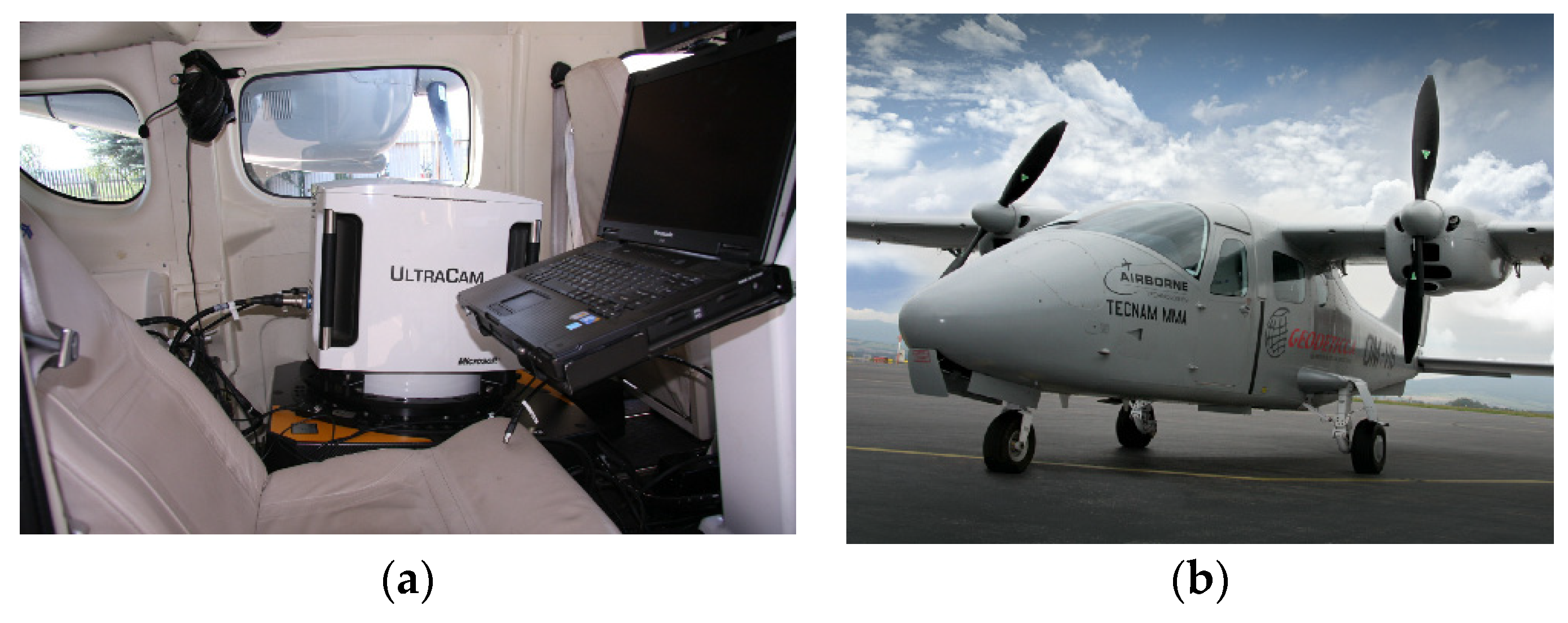
We consider aerial photogrammetry (AP) as a traditional surveying method. Compared to the aforementioned methods, it is suitable for larger territorial unit mapping or larger object documentation [19]. The most common products of aerial image processing are vector maps, orthophoto maps, digital terrain models (DTM), and digital surface models (DSM) [20,21,22]. In recent years, digital aerial cameras and appropriate software development have provided sensors with higher resolution, allowing the Earth’s surface to be captured with detail-level improvement at the same flight height, respectively reducing the necessary number of images and thus flight time and cost of imaging [23]. The minimizing of fieldwork time, rapidity of photogrammetric data collection and processing, and high detail and accuracy of the terrain models generated by modern software currently take aerial photogrammetry forward as an exciting alternative in terms of quality and efficiency in comparison with terrestrial geodetic methods [24].

Unmanned aerial systems (UAS) are preferred for smaller-scale areas today, mainly because of their ease of use and low acquisition costs.

Rusnák et al. provided a template for the application of unmanned aerial vehicles (UAV) in mapping a river landscape [25]. Its outputs can also be applied to the mapping and documentation of quarries and landfills. Zeybek [26], Štroner et al. [27], and Ren et al. [28] evaluated the quality and accuracy of UAV photogrammetry data using RTK GNSS methods. Without GCPs (ground control points), they achieved a positional accuracy of 1–3 cm and height accuracy of 4–6 cm. Burdziakowski addressed the quality of UAV-based DEM models affected by poor lighting conditions by comparing point clouds [29]. The filtering and classification of point clouds were dealt with by Zeybek [30] and Klápště et al. [31].

The analysis of spatial solids approximated by a regular solid was applied by Janowski et al. [32]. Speed and morphology change using cross-section processing was implemented by Kociuba [33]. Kociuba et al. in their works also dealt with the issue of the volume of moved material of eroded banks in Svalbard. They studied the bedload transport of material in a glacial river (see discussion) [34,35].

The current trend in photogrammetric processing is the SfM method. It can be used to process both terrestrial and aerial photogrammetric images [36]. In addition, there are many commercial and open-source software solutions [37].

Mapping using manned aerial systems is justified, especially for larger areas such as the tasks of investigating flood events [38], soil, gullies, shore erosion [39,40], landslides [41], and volcanological surveying [42] or of analysing the slope stability of hard-to-reach or larger units [43,44,45]. In practice, in addition to creating DEMs and DSMs, it is also used to create updates to orthophoto maps and large-scale maps. 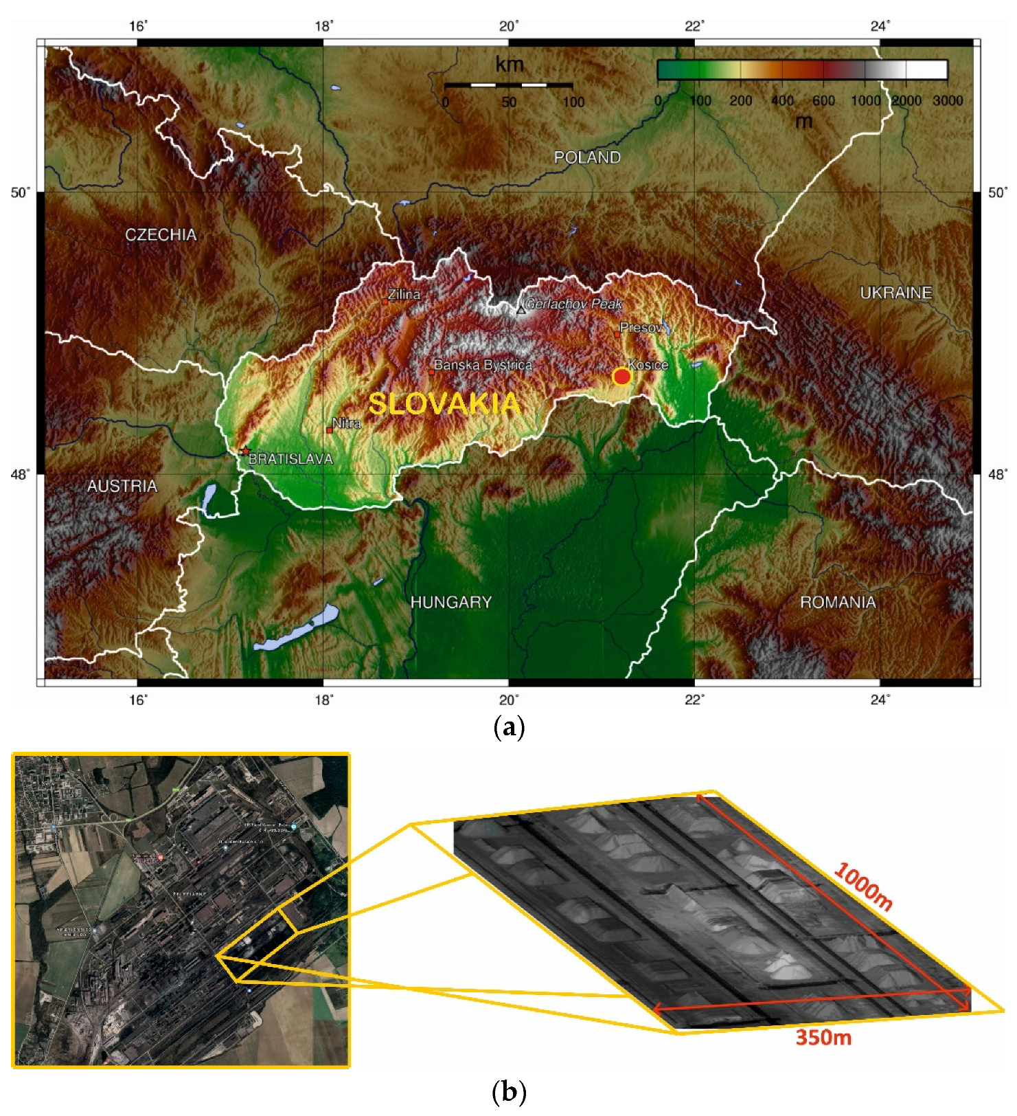Other types of sensors with their economic and technological benefits, such as thermal [46], multi, and hyperspectral cameras and Lidars [47,48,49,50,51,52], can also be placed on airborne platforms. The AP method using manned aerial vehicles is currently competing with the cheaper and more operational UAS photogrammetry, but it effectively covers a smaller area and takes measurements from a lower altitude. This study aims to demonstrate that the use of AP achieves the required accuracy and detail of outputs. After validation on a test area of 1000 m× 350 m, it can be assumed that usage in larger areas (open-pit mines, large landfills, etc.), i.e., where the use of conventional rotary or fixed-wing UAVs would be less economical, will meet the requirements and needs. We also see a use in obtaining data on industrial heaps and dumps as a secondary product when mapping larger parts of the territory if carried out in the required time.

Given the large range of the area of interest, the terrestrial measurement would force more days of shut down, which, at a frequent periodic measurement for the company operating in the area, represents an unacceptable loss of production. Therefore, from the available methods for performing the required measurements, the method of aerial photogrammetry has been chosen as likely the most appropriate way to fulfil the purpose of measurement. The advantages of this method consist of the very short time for measurement, fast and automated data processing procedures, sufficient precision, the non-contact method of measuring, and the minimized working time in the factory [3,18,23].

However, it was necessary to confirm the suitability of the digital aerial photogrammetry method as a primary method for future measurements regarding comparability and reliability of results with previous measurements. For this purpose, a one-time validation project of heap documentation and volume determination was realised with data collected by aerial photogrammetry compared to the reference method TLS and GNSS as previously used methods. This case study presents verifying the appropriateness of the photogrammetric techniques for the documentation and volume determining of material deposited in dumps of larger scale. The requirements for the measurement and processing methods are determined in particular by continuous operation in the plant (and therefore also in a landfill), the minimal forced shutdown of loaders, and the adequate accuracy of the determined volumes.

2. Materials and Methods

2.1. Study Area

Measurements were realized in the largest integrated iron and steel company in Eastern Slovakia near the town of Košice (Figure 1a). Dimensions of the study area at the time of measurements were approximately 1000 m × 350 m. There were 29 heaps of different materials of different shapes and sizes with a height of 10–15 m (Figure 1b). Two typical adjacent heaps were selected for this study.

2.2. Surveying Equipment

2.2.1. GNSS Receiver Leica GPS900CS

Dual-frequency GNSS rover Leica GPS 900CS equipped with hardware and software for receiving GPS and GLONASS signals was used. In this study, it was used in the coordinates of ground control points (GCP) determining the absolute orientation of photogrammetric images. Quick static GNSS method was used. Horizontal and vertical accuracy is expressed as follows according to the manufacturer data: standard deviation in position σ_p = 5 mm + 0.5 ppm and in height σ_h = 10 mm + 0.5 ppm. GNSS RTK measurement method was also used for the detailed measurement of two reference heap surfaces. Manufacturer declares horizontal and vertical accuracy in terms of relations σ_p = 10 mm + 1 ppm and σ_h = 20 mm + 1 ppm [53].

2.2.2. TLS Leica ScanStation C10

Reference measurement was made by the TLS Leica ScanStation C10 device with the rotating mirror along a horizontal axis. For distance measurement, the green 3R pulse visible laser with a wavelength of 532 nm is used. Standard deviation of single measured point position in the space is σ_p = 6 mm, standard deviation of distance measurement is σ_d = 4 mm (for lengths up to 50 m), standard deviations of horizontal directions and vertical angle measurement are σ_α = σ_z = 12’’, and precision of modelled surface is 2 mm. Range of measurement described by the manufacturer is 300 m at 90% reflectivity and 134 m at 18% reflectivity surface. Maximum measurement speed is up to 50,000 points per second. Field of view is 360° horizontal and 270° vertical [54].

2.2.3. Digital Aerial Photogrammetric Camera Microsoft UltraCamLp, Aircraft Tecnam MMA

Photogrammetric data collection was performed by digital aerial photogrammetric camera Microsoft UltraCamLp (Figure 2a). Image size is 11,704 × 7920 pixels, and output format is jpeg or tiff. Pixel size is 6 μm, and CCD chip area is 70.22 mm × 47.52 mm. Panchromatic lens has focal length of 70 mm. Field of view from vertical is 52° at the cross-track direction and 37° at along-track direction. Maximal image acquisition speed is one image per 2 s. Weight of the camera is about 55 kg [55]. The photogrammetric equipment carrier was a twin-propeller aircraft Tecnam MMA (Multi Mission Aircraft) (Figure 2b). Its length is 8.7 m, wingspan is 11.4 m, maximum takeoff weight is 1230 kg, and top speed is 145 knots [56]. The camera was mounted on an aircraft in a gyro-stabilizing basement, which significantly eliminates tilts of the aircraft. Aircraft technology was supplemented by GNSS and inertial measurement unit (IMU) in the product Applanix POSTrack ™, which stores the position and tilt of the camera at the time of exposure and provides input data for the calculation of the analytical aerotriangulation [57].

2.3. Data Acquisition and Processing

For the validation project of documentation and volume determination of bulk material heaps, surveying methods listed above were used. In addition, two neighbouring reference heaps were selected in which we assume the occurrence of error for points in a cloud, due to parts of the image that are too bright (overexposed) or fractions that are too soft (dust); thus, a smooth structure reduces the accuracy of the correlation, which was confirmed in the processing. For purposes of 3D model comparison, obtained by listed methods, the network of control points (CP) for terrestrial measurement and of ground control points (GCP) for aerial photogrammetry was created and surveyed. The coordinates of these points were determined in a common coordinate system ETRS 89 (European Terrestrial Reference System) by quick static method using relative GNSS measurements and transformed into the positional coordinate system S-JTSK (The Uniform Trigonometric Cadastral Network) and height system Bpv (Balt after adjustment). Both listed coordinate systems are used as a mandatory geodetic base in the Slovak Republic. Workflow diagram is shown in Figure 3. All field measurements and data acquisition GNSS, TLS, and AP were performed in one day during the shutdown of the production to prevent any changes in the morphology and size of the examined heaps.

2.3.1. GNSS Measurement

The GNSS measurement of selected heaps was carried out to compare the quality of measurements on the same day as TLS and AP data collection. RTK VRS method was used with a connection to a network of permanent reference stations, SKPOS^® serving as a base for relative measurements in the Slovak Republic. Virtual reference station was generated at the site of measurement. Positional accuracy of the measurement is indicated by the coordinate standard deviation σ_xy < 20 mm and height accuracy σ_h < 40 mm. At heap No. 1, 205 points were measured, and at heap No. 2, a total of 534 points.

2.3.2. Terrestrial Laser Scanning

Laser scanning was performed from six stations (Figure 4) at ground level (green mark) and one at an elevated level in the platform of the loading machine (blue mark). Georeferencing to the surveying network was carried out by the resection method. Network points (purple) were signalized by 6-inch targets for high-definition scanners (HDS) on tripods. The scanning resolution value was set to 5 cm at 100 m distance. For both heaps, 12.5 million points were measured (raw data) (Figure 5a). During the data processing, unnecessary and erroneous points in the scan were filtered, such as a loading machine, belt conveyors, error points, etc. (Figure 5b). Scanned data were further divided into single files for each heap and spatially subsampled to resolution of 5 cm. Resulting files contained approximately 181,000 points for heap No. 1 and 449,000 points for heap No. 2. Leica Cyclone 7.3^®, Microstation V8i^® with Terrascan v.13^®, and Trimble RealWorks 6.5^® software were used. Filtering and classification of the point cloud were performed as ground extraction in Terrascan^® software.

2.3.3. Aerial Photogrammetry

A priori analysis was performed to determine the expected accuracy of the determined volume. It depends mainly on the area of the surface and the accuracy of the height coordinates of the detailed points. When estimating the accuracy, a heap height of 10 m and the horizontal heap dimensions 100 m × 100 m were assumed. Photogrammetric software producer declares the standard height error of DSM points as 1.5 times the size of the pixels on the ground. If the maximum error does not exceed twice the mean error, and one pixel has a size of 5 cm, then the maximum difference in heap volume determining has a maximum value of 1.5%. Therefore, this accuracy is fully acceptable.

At the stage of flight plan creation for data collection, images with a resolution of 5 cm per pixel were proposed, which, regarding the parameters of the camera, corresponds to the flight altitude of 580 m above the ground. Four flight axes were realized (Figure 6). Mutual transverse overlap was 75%. Longitudinal overlap of images in the flight direction was 65%. Redundant number of frame pairs increases the accuracy of the resulting DSM and alternatively allows some images to be omitted: for example, blurred images due to turbulence during the flight.

Ten ground control points were stabilised for absolute image orientation in the coordinate system (Figure 6). GCPs were signalized by square black and white plastic signs with a size of approximately 30 cm× 30 cm. GCPs were determined by GNSS fast static method with post-processing and 20 min observation on each point. In addition, virtual reference station generated in the middle of the surveyed location (using SKPOS reference network data) was used.

Overall, 56 images were made in the case study area. Flight time between first and last image was approximately 15 min. The images were radiometrically corrected and calibrated. Data recorded by onboard GNSS receiver and IMU devices were post-processed and attached to the coordinate system ETRS89 and, together with the coordinates of control points and camera calibration parameters (internal orientation), provided input data for the block alignment of images and calculation of external orientation elements of the analytical aerotriangulation using photogrammetric software. The resulting coordinates were transformed into the coordinate system S-JTSK. Residual deviations of the ground control point coordinates after the analytical aerotriangulation solution reached values smaller than 20 mm for positional coordinates and 30 mm for the height coordinate.

From these modified aerial images, DSM was automatically generated in the form of a point cloud. Points were generated for every second pixel of the aerial image. About 1.7 million points (raw data) were processed. Unnecessary and erroneously generated points were filtered and removed similarly as described for TLS processing. Such modified point clouds contained about 168,000 points for Heap 1 and 445,000 points for Heap 2.

2.3.4. Data Processing

The single mesh models were created for every set of points obtained by the above-listed methods, which formed the upper terrain of selected heaps. Points bounding the heap and points on the ground plate have formed the lower terrain. Filtration removed erroneously generated (AP) and measured (TLS) points using Microstation software V8i^® with Terrascan v.13^®. Such modified point clouds are referenced and were the starting basis for the creation of final mesh models and further analysis. As the reference surfaces at both heaps, mesh models obtained by the TLS were considered.

For the purpose of compliance rate description of the compared surfaces, the Z coordinate differences were calculated. Applying the AP and GNSS methods, obtained data were compared with the reference model (TLS).

Residuals represent the vertical difference between the Z value in the data file and the interpolated Z value on a reference surface at every position X, Y of the data file point. In this case, the bilinear interpolation method was used.

The formula used to compute a residual value is

$$Z_{res}=Z_{dat}-Z_{ref},$$

(1)

where: $Z_{res}$ is the difference value, $Z_{dat}$ is the Z value in the compared data file, and $Z_{ref}$ is the interpolated Z value on the surface at each X, Y point coordinate on the reference surface.

The standard deviation σ of the data file is the square root of the variance of the file and is, in general, calculated by the formula

$$\sigma =\sqrt{\frac{1}{\left(n-1\right)}{\displaystyle \sum _{i=1}^n{\left(z_i-\overline{z}\right)}^2}},$$

(2)

where: $n$ is the number of observations, $z_i$ is the data value, and $\overline{z}$ is the mean.

Creation of the cross-sections was performed by the Surfer^® software. For both heaps, three vertical sections parallel to each other were created (Figure 7). They were situated parallel to the longest dimension of the heap in the heap centre and its side slopes. In each section, about 120 data points were evaluated without removing outliers. As the reference surface, the model surveyed by the TLS method was chosen.

3. Results

The main characteristics of the created point clouds are listed in

Table 1. Characteristics of point clouds: Heap No. 1.

Method	No. of Points	No. of Triangles in Mesh	Density of Points	Average Distance between Points
GNSS RTK	205	377	0.1/m2	3 m
TLS	181 360	362 524	196/m2	0.07 m
AP	168 084	335 826	100/m2	0.10 m

and

Table 2. Characteristics of point clouds: Heap No. 2.

Method	No. of Points	No. of Triangles in Mesh	Density of Points	Average Distance between Points
GNSS RTK	534	1 034	0.1/m2	3 m
TLS	449 404	898 551	196/m2	0.07 m
AP	446 629	891 591	100/m2	0.10 m

.

3.1. Analysis of Surfaces

The Trimble Realworks^® ver. 11.3. software was used for the twin surface comparison as a coloured mesh with differential scale (Figure 8). The comparison expresses the compliance rate of the compared surfaces.

Regarding the large number of evaluated points, the compliance differences of the compared surface residuals were evaluated graphically as a frequency histogram, where on the X axis, the intervals of residuals are displayed, and on the Y axis, the frequency of residuals in intervals from −0.2 m to + 0.2 m are displayed (Figure 9). The single bin size was set to 5 mm; the number of intervals was therefore 80. The values of residuals of TLS vs. AP (Figure 9a,c) were determined as processed for two separate heaps. Then, as a result, the correlation coefficient 0.96 was calculated. For TLS vs. GNSS values of residuals (Figure 9b,d), the correlation coefficient value was 0.75.

Table 3. Surface differences evaluation—Heap No. 1.

Heap 1	Frequency of Residuals for Compared Surfaces in Intervals
	up to ±20 mm	up to ±40 mm	up to ±60 mm	up to ±80 mm
TLS vs. AP	53%	73%	78%	92%
TLS vs. GNSS	18%	30%	53%	72%

and

Table 4. Surface differences evaluation—Heap No. 2.

Heap 2	Frequency of Residuals for Compared Surfaces in Intervals
	up to ±20 mm	up to ±40 mm	up to ±60 mm	up to ±80 mm
TLS vs. AP	44%	73%	80%	92%
TLS vs. GNSS	21%	40%	53%	73%

show the percentage frequency of points at intervals up to ±20 mm, ±40 mm, ±60 mm, and ±80 mm based on residual differences of surfaces obtained by the selected surveying methods.

3.2. Analysis of Cross-Sections

Table 5. Cross-sections differences evaluation—Heap No. 1.

Heap 1	Frequency of Residuals in Compared Cuts in Intervals
	up to ±20 mm	up to ±40 mm	up to ±60 mm	up to ±80 mm
TLS vs. AP	57%	72%	80%	91%
TLS vs. GNSS	16%	31%	50%	67%

and

Table 6. Cross-sections differences evaluation—Heap No. 2.

Heap 2	Frequency of Residuals in Compared Cuts in Intervals
	up to ±20 mm	up to ±40 mm	up to ±60 mm	up to ±80 mm
TLS vs. AP	42%	73%	85%	93%
TLS vs. GNSS	17%	39%	55%	72%

show the percentage frequency of points at intervals up to ±20 mm, ±40 mm, ±60 mm, and ±80 mm based on residual differences of surfaces in cross-sections obtained by the selected surveying methods. The cross-sections comparison result of surfaces obtained by the AP and GNSS methods represents the data file in which the height differences against the reference surface were contained.

A graphical representation of these differences in sections for the surfaces obtained by the AP and GNSS methods is presented (Figure 10).

3.3. Analysis of Volumes

The volume calculation was realized for each heap and method separately. The upper surface was formed by the heap body points, while the lower surface was created by points on the ground plate in the heap surrounding. Volumes were therefore determined independently on the mutual registration of point files. Volume calculation was performed by the Trimble Realworks^® software. The designated volume and the absolute and percentage comparison are shown in

Table 7. Volume differences comparison.

Heap	Surveying Method	Volume (m3)	Volume Difference (m3) (%)
Heap 1	TLS	4584	-	-
	AP	4588	4	0.09
	GNSS	4430	−154	−3.36
Heap 2	TLS		-	-
	AP		14	0.08
	GNSS		−311	−1.67

.

4. Discussion

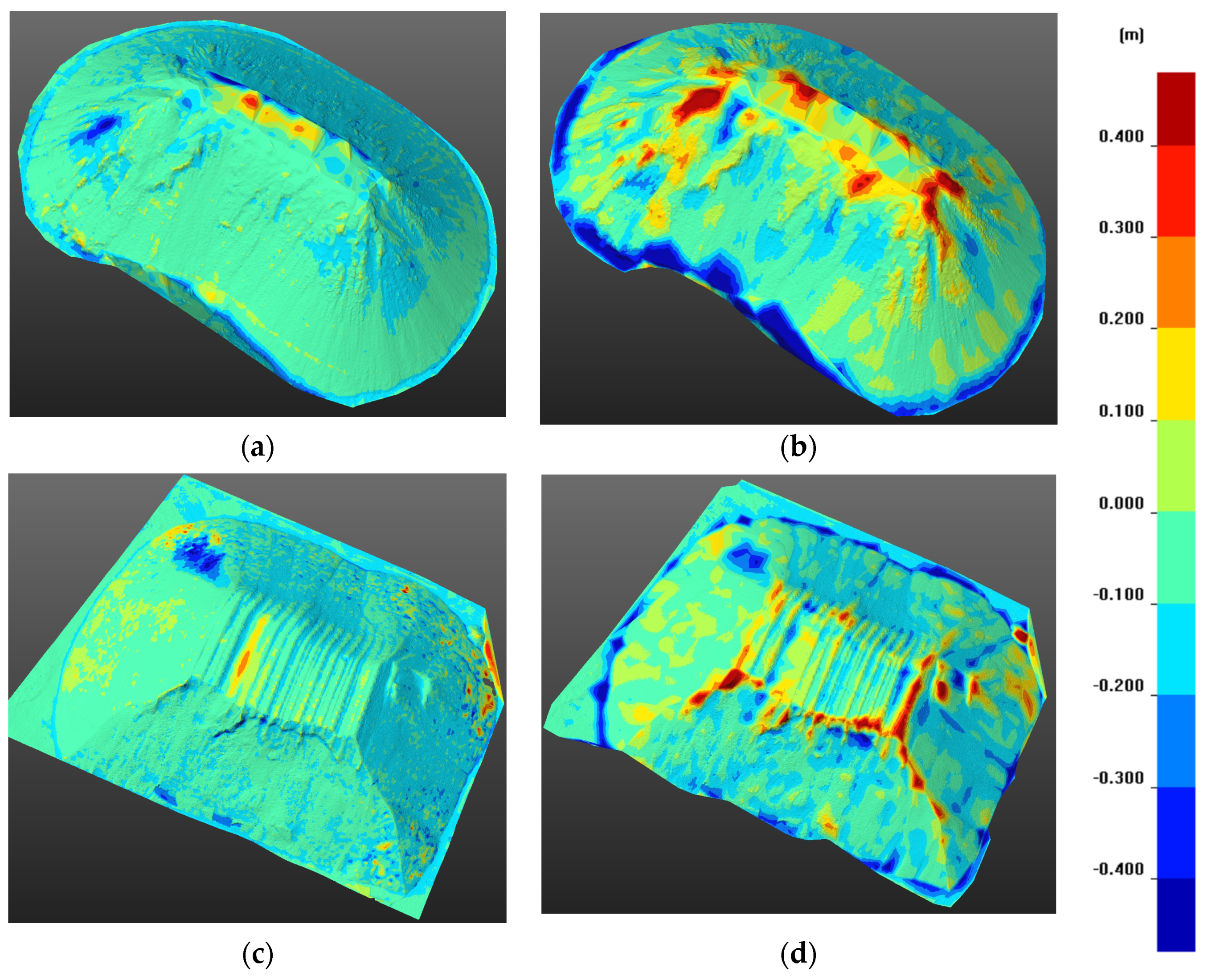
The mesh surface comparison (Figure 8) was the initial analysis in this research. It shows a level of agreement of the compared surfaces obtained by different surveying methods. TLS vs. AP surface evaluation (Figure 8a,c) is almost identical at both heaps. The most significant differences between the surfaces were detected mainly on the upper part of the heap and partly on its sidewalls (red and blue colours). This can be assigned to the absence of a sufficient number of points at these locations measured by the TLS method. Despite the goal of making TLS measurements with a full coverage of heaps and with a raised instrument station position, these areas were hidden by obstacles. The TLS vs. GNSS surface comparison (Figure 8b,d) identifies significant differences of surfaces at both heaps. These are mainly found on the edges of the formed planar areas and on the circumference at the base of the heaps. This is due to the substantially lower density of points in the model created from the GNSS RTK measurements. Furthermore, all the direct methods, including GNSS, are influenced by human factors: when moving on the heap, it is not easy for the operator to select the appropriate measured points for optimal surface description.

To obtain numerical values for comparison, the frequency difference histograms were created in sets with a 5 mm size for the residual values of −0.2 m to + 0.2 m (Figure 9). TLS vs. AP surface analysis has confirmed the initial assumption about the possible correlation of surface models obtained by the employed method. TLS vs. AP surface validation shows a standard deviation σ = 39 mm for Heap no. 1 and σ = 42 mm for Heap No. 2. TLS vs. GNSS surface validation shows a standard deviation σ = 67 mm for Heap no. 1 and σ = 68 mm for Heap No. 2. When comparing the TLS vs. AP surface validation residuals, there is a mean error value of 9 mm for Heap No. 1 and 6 mm for Heap No. 2. TLS vs. GNSS surface validation residuals show a mean error value of 12 mm for Heap No. 1 and a mean error value of 15 mm for Heap No. 2. The correlation coefficient was calculated from the frequency of residual values at the selected intervals of 5 mm of the same data collection methods and processed in two separate heaps. The correlation coefficient value was 0.96 for the AP and 0.75 for the GNSS measurement. This parameter shows a high reliability, especially for the results obtained by the AP.

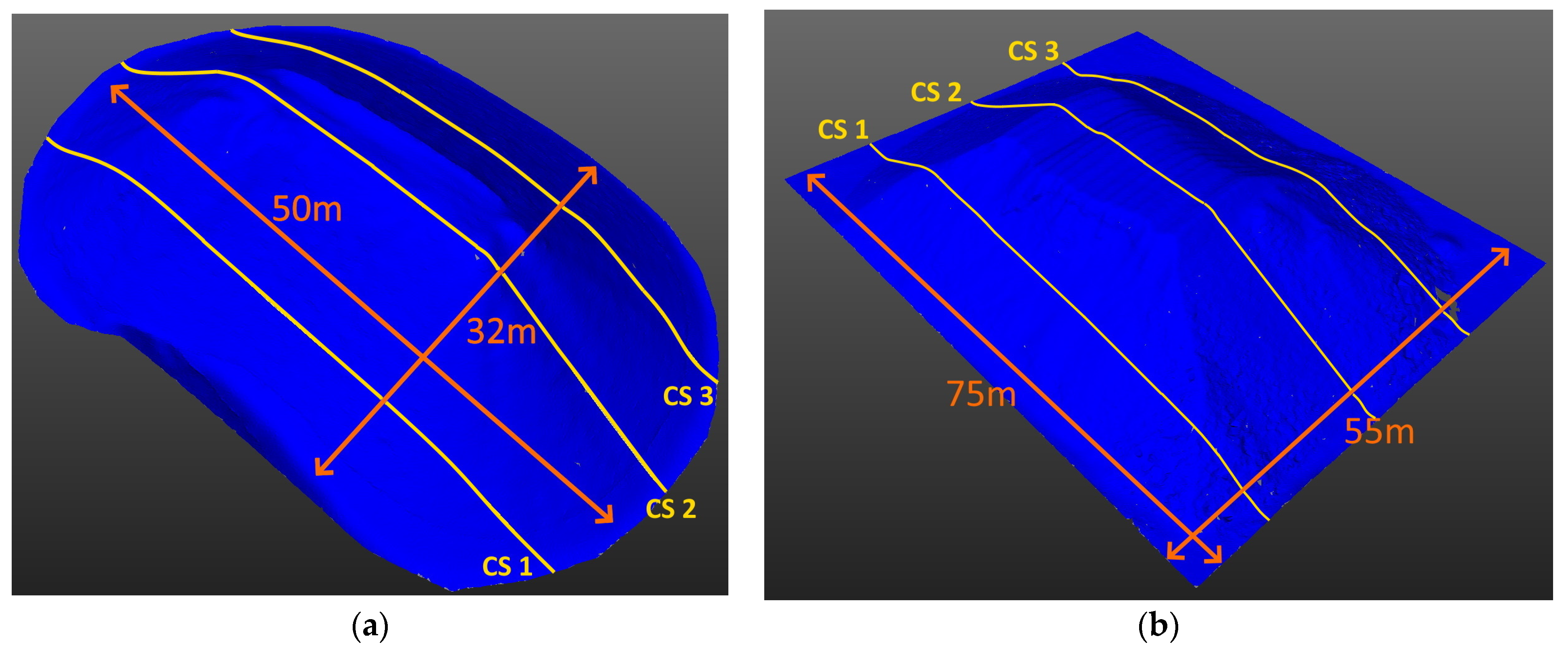
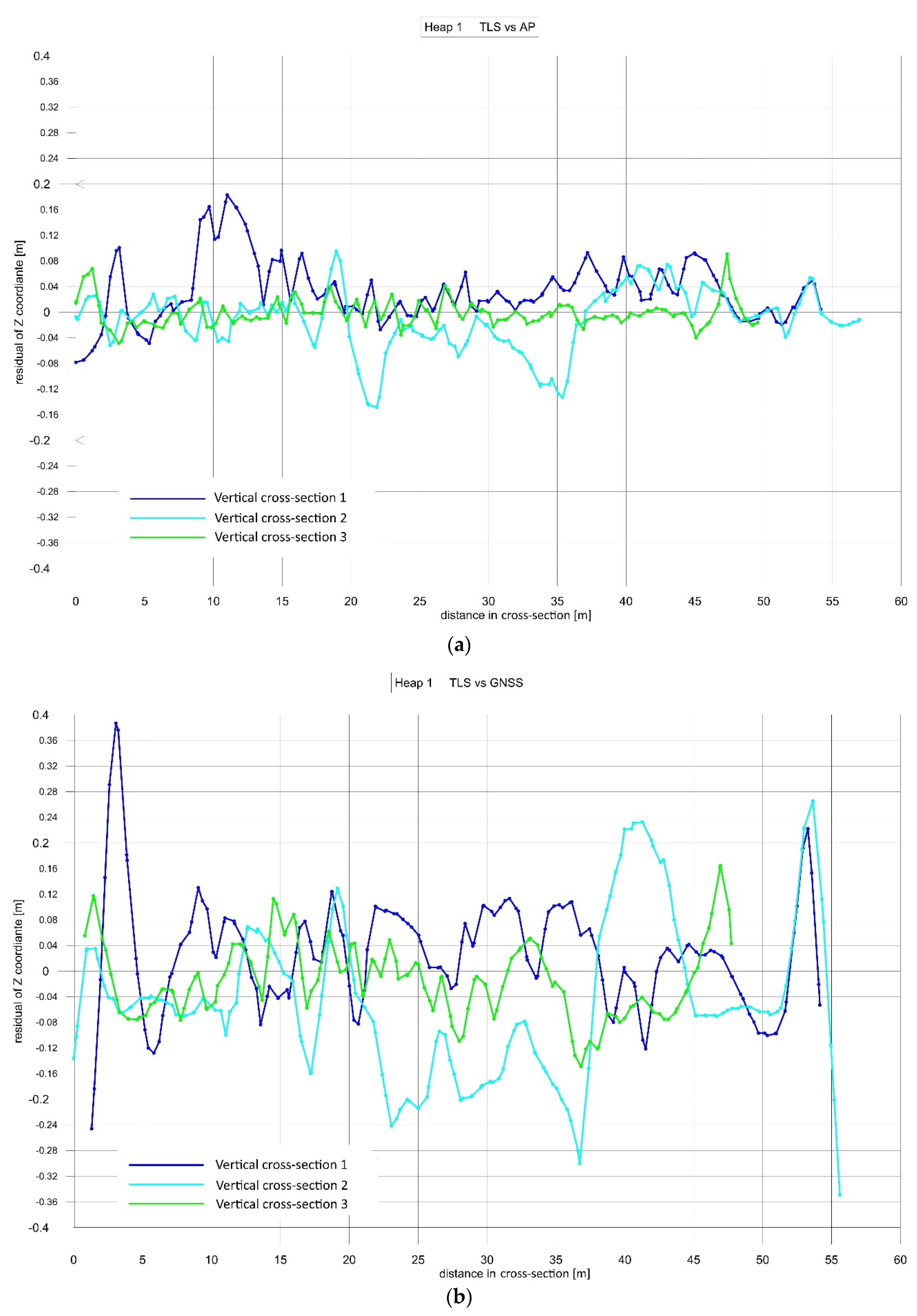
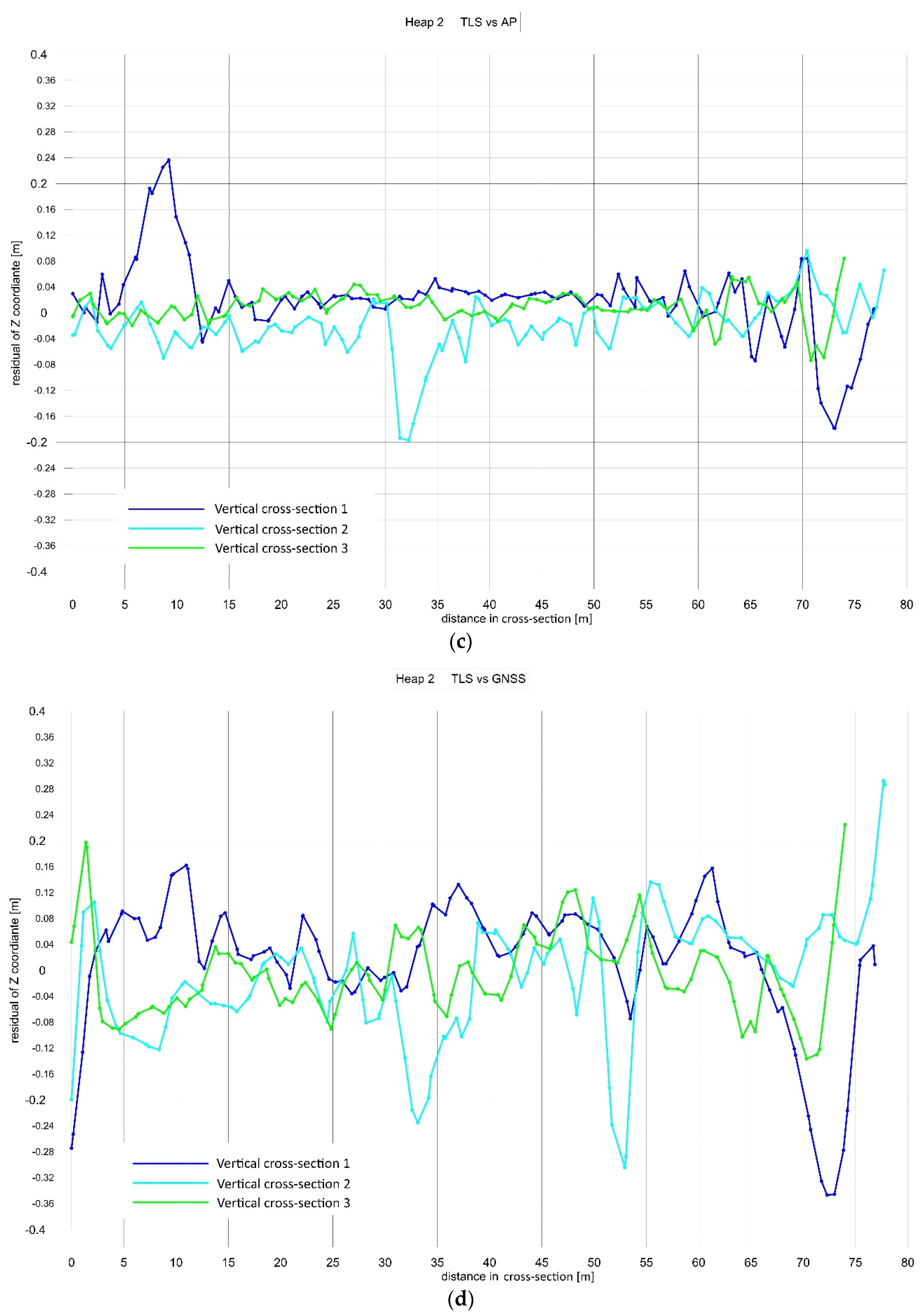
Cross-section analysis (Figure 10) was performed on smaller datasets relative to surface analysis, which corresponds to the evaluated standard deviations according to initial assumptions. TLS vs. AP cross-sections validation has a standard deviation σ = 53 mm for Heap No. 1 and σ = 49 mm for Heap No. 2. TLS vs. GNSS surface validation shows a standard deviation σ = 100 mm for Heap No. 1 and σ = 91 mm for Heap No. 2. TLS vs. AP cross-sections validation residuals show a mean value $\overline{z}$ = 6 mm for Heap No. 1 and $\overline{z}$ = 3 mm for Heap No. 2. TLS vs. GNSS surface validation shows a mean value $\overline{z}$ = 11 mm for Heap No. 1 and $\overline{z}$ = 8 mm for Heap No. 2.

Yourtseven [58] compared photogrammetric DSMs obtained from different flight altitudes up to 350 m AGL using UAS. The reference model was DSM obtained by TLS. When comparing GNSS and TLS measurements by comparing the Z coordinate in the sections, he achieved a standard deviation of 73 mm. When comparing GNSS and AP from a height of 350 m AGL, the standard deviation was approximately 60 mm. The values correspond to our achieved results. When comparing TLS and AP, a standard deviation value of up to 76 mm was reached.

The comparison of the specified volumes (Table 7) confirms the results of previous analyses. Volume difference values were specified for the comparison of TLS vs. AP as 0.09% at Heap No. 1 and 0.08% at Heap No. 2, and for the comparison of TLS vs. GNSS as −3.36% for Heap No. 1 and −1.67% for Heap No. 2. Regarding the relatively large size difference of both heaps, these results are at the level of expected values and correspond to small values of the mean error of residuals to the reference surface.

The determination of volumes by contact methods such as the spatial polar method using total stations and the RTK method using GNSS was summarized by Ajayi [3] as comparable. This is mainly due to approximately the same density of measured points. This has the most significant impact on the quality of the model and the derived results. By comparing volumes with a reference value, he determined an error in determining the volume with a value of 2.9% [3], which is in line with our results of the GNSS comparison. Tamin et al. [59] achieved a volume difference of 0.002% between TLS and AP. For AP data acquisition, a UAS was used at the height of 100 m AGL.

The results show that the AP method for volume determination and documentation is in its precision comparable with the reference method TLS (the calculated volumes differ by less than 0.1%) and is significantly more accurate and reliable than the RTK GNSS method (volumes differ in ones of percentages).

The advantage is the high density of surveyed points and thus almost true shape capture of the measured object. In areas with poorer texture, e.g., smooth surfaces and shadowy places, the error points occur, but these can be effectively removed using appropriate filtering tools. In the case of multistage measurements, it is appropriate to make a flight with the same parameters and external orientation using the same control points [60].

Although the TLS measurement method achieves excellent results, it has some limits: in particular, the need for field measurements and the incompleteness of the point cloud and 3D model. It is, therefore, suitable for smaller areas or separate objects [34]. Furthermore, the AP method with a correct measurement setup provides a higher work efficiency and model quality [5,17].

Ajayi [3] also compared the time required for field measurements by the different methods. If we do not consider the time required for flight and GCP preparation, conventional measurement is more time consuming than AP. In our case study, a large area was surveyed. Therefore, fieldwork is only a small part of the surveying process. The total time required for AP acquisition is, then, shorter than using terrestrial measurement [36]. However, with a large number of images, it is necessary to take into account the longer time of post-processing software processing [37].

A disadvantage of AP use is that it only allows for measuring objects visible from above. It depends on suitable weather, which allows the flight to be made and provides good lighting conditions. Measurements can be made only in daylight, ideally in the midday hours. Risk factors in terms of industrial plants also include the direction and strength of the wind, which could impair visibility by smoke from nearby chimneys or swirling dust from heaps. These risks should be considered during mission planning and scheduling. Nevertheless, the accuracy, efficiency, speed, and economic view of AP compared with other methods make it the first choice for solving problems associated with data collection for terrain modelling and volume calculation with larger scale territory and objects.

5. Conclusions

The presented validation study aimed to compare the modern geodetic technologies TLS and AP for determining the volume of heaps of material and their spatial documentation. In addition, the GNSS RTK method and TLS were also compared to bind actual measurements with previously used surveying methods. As the reference method, TLS was chosen because of the high density, the number of measured points, and the high measuring accuracy.

AP measurements are very fast and can cover a large area in a short time and from a high flight altitude (even compared to UAVs). The time required for fieldwork in comparison with conventional surveying techniques is markedly shorter. The method is therefore also suitable when dynamic change detection in a short time is needed. The measurement is non-contact, and thus it can be safely implemented even in harmful or hazardous environments.

References

1. Khanal, M.; Hasan, M.; Sterbentz, N.; Johnson, R.; Weatherly, J. Accuracy Comparison of Aerial Lidar, Mobile-Terrestrial Lidar, and UAV Photogrammetric Capture Data Elevations over Different Terrain Types. Infrastructures 2020, 5, 65. [Google Scholar] [CrossRef]
2. Grottoli, E.; Biausque, M.; Rogers, D.; Jackson, D.W.T.; Cooper, J.A.G. Structure-from-Motion-Derived Digital Surface Models from Historical Aerial Photographs: A New 3D Application for Coastal Dune Monitoring. Remote Sens. 2021, 13, 95. [Google Scholar] [CrossRef]
3. Ajayi, O.; Ajulo, J. Investigating the Applicability of Unmanned Aerial Vehicles (UAV) Photogrammetry for the Estimation of the Volume of Stockpiles. Quaest. Geogr. 2021, 40, 25–38. [Google Scholar] [CrossRef]
4. Kovanič, Ľ. Possibilities of Terrestrial Laser Scanning Method in Monitoring of Shape Deformation in Mining Plants. Inżynieria Miner. J. Pol. Miner. Eng. Soc. 2013, 1, 29–41. [Google Scholar]
5. Urban, R.; Štroner, M.; Blistan, P.; Kovanič, Ľ.; Patera, M.; Jacko, S.; Ďuriška, I.; Kelemen, M.; Szabo, S. The Suitability of UAS for Mass Movement Monitoring Caused by Torrential Rainfall—A Study on the Talus Cones in the Alpine Terrain in High Tatras, Slovakia. ISPRS Int. J. Geo-Inf. 2019, 8, 317. [Google Scholar] [CrossRef] [Green Version]
6. Kovanič, Ľ.; Blistan, P.; Urban, R.; Štroner, M.; Blišťanová, M.; Bartoš, K.; Pukanská, K. Analysis of the Suitability of High-Resolution DEM Obtained Using ALS and UAS (SfM) for the Identification of Changes and Monitoring the Development of Selected Geohazards in the Alpine Environment—A Case Study in High Tatras, Slovakia. Remote Sens. 2020, 12, 3901. [Google Scholar] [CrossRef]
7. Gallay, M.; Hochmuth, Z.; Kaňuk, J.; Hofierka, J. Geomorphometric analysis of cave ceiling channels mapped with 3-D terrestrial laser scanning. Hydrol. Earth Syst. Sci. 2016, 20, 1827–1849. [Google Scholar] [CrossRef] [Green Version]
8. Hofierka, J.; Gallay, M.; Kaňuk, J.; Šašak, J. Modelling Karst Landscape with Massive Airborne and Terrestrial Laser Scanning Data. In The Rise of Big Spatial Data. Lecture Notes in Geoinformation and Cartography; Ivan, I., Singleton, A., Horák, J., Inspektor, T., Eds.; Springer: Cham, Switzerland, 2017. [Google Scholar]
9. Pukanská, K.; Bartoš, K.; Bella, P.; Gašinec, J.; Blistan, P.; Kovanič, Ľ. Surveying and High-Resolution Topography of the Ochtiná Aragonite Cave Based on TLS and Digital Photogrammetry. Appl. Sci. 2020, 10, 4633. [Google Scholar] [CrossRef]
10. Erdélyi, J.; Kopáčik, A.; Kyrinovič, P. Construction control and documentation of facade elements using terrestrial laser scanning. Appl. Geomat. 2018, 10, 113–121. [Google Scholar] [CrossRef]
11. Erdélyi, J.; Kopáčik, A.; Kyrinovič, P. Spatial Data Analysis for Deformation Monitoring of Bridge Structures. Appl. Sci. 2020, 10, 8731. [Google Scholar] [CrossRef]
12. Kovanič, Ľ.; Blistan, P.; Urban, R.; Štroner, M.; Pukanská, K.; Bartoš, K.; Palková, J. Analytical Determination of Geometric Parameters of the Rotary Kiln by Novel Approach of TLS Point Cloud Segmentation. Appl. Sci. 2020, 10, 7652. [Google Scholar] [CrossRef]
13. Malowany, K.; Magda, K.; Rutkiewicz, J.; Malesa, M.; Kantor, J.; Michoński, J.; Kujawińska, M. Measurements of geometry of a boiler drum by time-of-flight laser scanning. Measurement 2015, 72, 88–95. [Google Scholar] [CrossRef]
14. Blistan, P.; Jacko, S.; Kovanič, Ľ.; Kondela, J.; Pukanská, K.; Bartoš, K. TLS and SfM Approach for Bulk Density Determination of Excavated Heterogeneous Raw Materials. Minerals 2020, 10, 174. [Google Scholar] [CrossRef] [Green Version]
15. Křemen, T. Measurement and documentation of St. Spirit Church in Liběchov. In Advances and Trends in Geodesy, Cartography amd Geoinformatics II; CRC Press: Boca Raton, FL, USA, 2020; pp. 44–49. ISBN 978-0-367-34651-5. [Google Scholar]
16. Křemen, T. Documentation of the main tower of the medieval castle. In Proceedings of the 17th International Multidisciplinary Scientific GeoConference SGEM 2017, Albena, Bulgaria, 29 June–5 July 2017; pp. 265–272, ISBN 978-619-7408-02-07. [Google Scholar]
17. Koska, B.; Křemen, T. The Combination of Laser Scanning and Structure from Motion Technology for Creation of Accurate Exterior and Interior Orthophotos of St. Nicholas Baroque Church. ISPRS Int. Arch. Photogramm. Remote Sens. Spat. Inf. Sci. 2013, 40, 133–138. [Google Scholar] [CrossRef] [Green Version]
18. Janowski, A.; Nagrodzka-Godycka, K.; Szulwic, J.; Ziolkowski, P. Remote sensing and photogrammetry techniques in diagnostics of concrete structures. Comput. Concr. 2016, 18, 405–420. [Google Scholar] [CrossRef] [Green Version]
19. Conte, P.; Girelli, V.A.; Mandanici, E. Structure from Motion for aerial thermal imagery at city scale: Pre-processing, camera calibration, accuracy assessment. ISPRS J. Photogramm. Remote Sens. 2018, 146, 320–333. [Google Scholar] [CrossRef]
20. Nolan, M.; Larsen, C.; Sturm, M. Mapping snow depth from manned aircraft on landscape scales at centimeter resolution using structure-from-motion photogrammetry. Cryosphere 2015, 9, 1445–1463. [Google Scholar] [CrossRef] [Green Version]
21. Szabó, S.; Enyedi, P.; Horváth, M.; Kovács, Z.; Burai, P.; Csoknyai, T.; Szabó, G. Automated registration of potential locations for solar energy production with Light Detection And Ranging (LiDAR) and small format photogrammetry. J. Clean. Prod. 2016, 112, 3820–3829. [Google Scholar] [CrossRef]
22. Wang, J.; Wang, L.; Jia, M.; He, Z.; Bi, L. Construction and optimization method of the open-pit mine DEM based on the oblique photogrammetry generated DSM. Measurement 2020, 152, 107322. [Google Scholar] [CrossRef]
23. Mielcarek, M.; Kamińska, A.; Stereńczak, K. Digital Aerial Photogrammetry (DAP) and Airborne Laser Scanning (ALS) as Sources of Information about Tree Height: Comparisons of the Accuracy of Remote Sensing Methods for Tree Height Estimation. Remote Sens. 2020, 12, 1808. [Google Scholar] [CrossRef]
24. Enríquez, C.; Jurado, J.M.; Bailey, A.; Callén, D.; Collado, M.J.; Espina, G.; Marroquín, P.; Oliva, E.; Osla, E.; Ramos, M.I.; et al. The UAS-Based 3D Image Characterization of Mozarabic Church Ruins in Bobastro (Malaga), Spain. Remote Sens. 2020, 12, 2377. [Google Scholar] [CrossRef]
25. Rusnák, M.; Sládek, J.; Kidová, A.; Lehotský, M. Template for high-resolution river landscape mapping using UAV technology. Measurement 2018, 115, 139–151. [Google Scholar] [CrossRef]
26. Zeybek, M. Accuracy assessment of direct georeferencing UAV images with onboard global navigation satellite system and comparison of CORS/RTK surveying methods. Meas. Sci. Technol. 2021, 32, 065402. [Google Scholar] [CrossRef]
27. Štroner, M.; Urban, R.; Seidl, J.; Reindl, T.; Brouček, J. Photogrammetry Using UAV-Mounted GNSS RTK: Georeferencing Strategies without GCPs. Remote Sens. 2021, 13, 1336. [Google Scholar] [CrossRef]
28. Ren, H.; Zhao, Y.; Xiao, W.; Wang, X.; Sui, T. An Improved Ground Control Point Configuration for Digital Surface Model Construction in a Coal Waste Dump Using an Unmanned Aerial Vehicle System. Remote Sens. 2020, 12, 1623. [Google Scholar] [CrossRef]
29. Burdziakowski, P.; Bobkowska, K. UAV Photogrammetry under Poor Lighting Conditions—Accuracy Considerations. Sensors 2021, 21, 3531. [Google Scholar] [CrossRef]
30. Zeybek, M.; Şanlıoğlu, I. Point cloud filtering on UAV based point cloud. Measurement 2019, 133, 99–111. [Google Scholar] [CrossRef]
31. Klápště, P.; Fogl, M.; Barták, V.; Gdulová, K.; Urban, R.; Moudrý, V. Sensitivity analysis of parameters and contrasting performance of ground filtering algorithms with UAV photogrammetry-based and LiDAR point clouds. Int. J. Digit. Earth 2020, 13, 1672–1694. [Google Scholar] [CrossRef]
32. Janowski, A.; Bobkowska, K.; Szulwic, J. 3D modelling of cylindrical-shaped objects from lidar data—An assessment based on theoretical modellingand experimental data. Metrol. Meas. Syst. 2018, 25, 1. [Google Scholar] [CrossRef]
33. Kociuba, W.; Janicki, G. Effect of Meteorological Patterns on the Intensity of Streambank Erosion in a Proglacial Gravel-Bed River (Spitsbergen). Water 2018, 10, 320. [Google Scholar] [CrossRef] [Green Version]
34. Kociuba, W.; Kubisz, W.; Zagórski, P. Use of terrestrial laser scanning (TLS) for monitoring and modelling of geomorphic processes and phenomena at a small and medium spatial scale in Polar environment (Scott River—Spitsbergen). Geomorphology 2014, 212, 84–96. [Google Scholar] [CrossRef]
35. Kociuba, W.; Janicki, G. Continuous measurements of bedload transport rates in a small glacial river catchment in the summer season (Spitsbergen). Geomorphology 2014, 212, 58–71. [Google Scholar] [CrossRef]
36. Pukanská, K.; Bartoš, K.; Sabová, J. Comparison of Survey Results of the Surface Quarry Spišské Tomášovce by the Use of Photogrammetry and Terrestrial Laser Scanning. Inżynieria Miner. 2014, 33, 47–54. [Google Scholar]
37. Bartoš, K.; Pukanská, K.; Sabová, J. The Analysis, Accuracy and Utilization of Open-Source Photogrammetric software. Inżynieria Miner. 2014, 60, 299–306. [Google Scholar]
38. Park, K.; Shibuo, Y.; Katayama, J.; Baba, S.; Furumai, H. Applicability of High-Resolution Geospatial Data Obtained by UAV Photogrammetry to Develop Drainage System Models for Pluvial Flood Analysis. J. Disaster Res. 2021, 16, 371–380. [Google Scholar] [CrossRef]
39. Kaiser, A.; Neugirg, F.; Rock, G.; Müller, C.; Haas, F.; Ries, J.; Schmidt, J. Small-Scale Surface Reconstruction and Volume Calculation of Soil Erosion in Complex Moroccan Gully Morphology Using Structure from Motion. Remote Sens. 2014, 6, 7050–7080. [Google Scholar] [CrossRef] [Green Version]
40. Suo, C.; McGovern, E.; Gilmer, A.; Cahalane, C. A comparison of high-end methods for topographic modelling of a coastal dune complex. J Coast Conserv. 2020, 24, 47. [Google Scholar] [CrossRef]
41. Fernández, T.; Pérez-García, J.L.; Gómez-López, J.M.; Cardenal, J.; Moya, F.; Delgado, J. Multitemporal Landslide Inventory and Activity Analysis by Means of Aerial Photogrammetry and LiDAR Techniques in an Area of Southern Spain. Remote Sens. 2021, 13, 2110. [Google Scholar] [CrossRef]
42. Pesci, A.; Fabris, M.; Conforti, D.; Loddo, F.; Baldi, P.; Anzidei, M. Integration of ground-based laser scanner and aerial digital photogrammetry for topographic modelling of Vesuvio volcano. J. Volcanol. Geotherm. Res. 2007, 162, 123–138. [Google Scholar] [CrossRef]
43. Salvini, R.; Francioni, M.; Riccucci, S.; Bonciani, F.; Callegari, I. Photogrammetry and laser scanning for analyzing slope stability and rock fall runout along the Domodossola-Iselle railway, the Italian Alps. Geomorphology 2013, 185, 110–122. [Google Scholar] [CrossRef]
44. Lai, H.; Liu, L.; Liu, X.; Zhang, Y.; Xuan, X. Unmanned aerial vehicle oblique photography-based superposed fold analysis of outcrops in the Xuhuai region, North China. Geol. J. 2021, 56, 2212–2222. [Google Scholar] [CrossRef]
45. Park, S.; Choi, Y. Applications of Unmanned Aerial Vehicles in Mining from Exploration to Reclamation: A Review. Minerals 2020, 10, 663. [Google Scholar] [CrossRef]
46. Jon, J.; Koska, B.; Pospíšil, J. Autonomous Airship Equipped with Multi-Sensor Mapping Platform. ISPRS Int. Arch. Photogramm. Remote Sens. Spat. Inf. Sci. 2013, 40, 119–124. [Google Scholar] [CrossRef] [Green Version]
47. Pellicani, R.; Argentiero, I.; Manzari, P.; Spilotro, G.; Marzo, C.; Ermini, R.; Apollonio, C. UAS and Airborne LiDAR Data for Interpreting Kinematic Evolution of Landslide Movements: The Case Study of the Montescaglioso Landslide (Southern Italy). Geosciences 2019, 9, 248. [Google Scholar] [CrossRef] [Green Version]
48. Salach, A.; Bakuła, K.; Pilarska, M.; Ostrowski, W.; Górski, K.; Kurczyński, Z. Accuracy Assessment of Point Clouds from LiDAR and Dense Image Matching Acquired Using the UAS Platform for DTM Creation. ISPRS Int. J. Geo-Inf. 2018, 7, 342. [Google Scholar] [CrossRef] [Green Version]
49. Kociuba, W. Different Paths for Developing Terrestrial LiDAR Data for Comparative Analyses of Topographic Surface Changes. Appl. Sci. 2020, 10, 7409. [Google Scholar] [CrossRef]
50. Siwiec, J. Comparison of Airborne Laser Scanning of Low and High Above Ground Level for Selected Infrastructure Objects. J. Appl. Eng. Sci. 2018, 8, 89–96. [Google Scholar] [CrossRef] [Green Version]
51. Cech, J.; Sofranko, M. Economic projection and evaluation of mining venture. Econ. Manag. 2018, 21, 2. [Google Scholar] [CrossRef]
52. Behun, M.; Kascak, P.; Hrabcak, M.; Behunova, A.; Knapcikova, L.; Sofranko, M. Investigation of Sustainable Geopolymer Composite Using Automatic Identification Technology. Sustainability 2020, 12, 6377. [Google Scholar] [CrossRef]
53. Available online: https://www.geotech.sk/downloads/GPS/GPS900CS/Leica_GPS900CS_prospekt_SK.pdf (accessed on 10 June 2021).
54. Available online: https://www.geotech.sk/downloads/Laserove-skenery-HDS/Leica_ScanStation_C10_Brochure_sk.pdf (accessed on 10 June 2021).
55. Available online: http://download.microsoft.com/download/2/E/7/2E7FCE24-E085-4A64-B568-25BA956FCB60/UltraCamSpecifications_UCD_UCX_UCXp_UCXpWA_UCL_UCLp.pdf (accessed on 10 June 2021).
56. Available online: https://www.airbornetechnologies.at/images/neu/media/downloads/Folder_Tecnam_MMA.pdf (accessed on 10 June 2021).
57. Available online: https://www.applanix.com/products/postrack.htm (accessed on 10 June 2021).
58. Yurtseven, H. Comparison of GNSS-, TLS- and Different Altitude UAV-Generated Datasets on the Basis of Spatial Differences. ISPRS Int. J. Geo-Inf. 2019, 8, 175. [Google Scholar] [CrossRef] [Green Version]
59. Tamin, M.A.; Darwin, N.; Majid, Z.; Ariff, M.F.M.; Idris, K.M.; Samad, A.M. Volume Estimation of Stockpile Using Unmanned Aerial Vehicle. In Proceedings of the 9th IEEE International Conference on Control System, Computing and Engineering (ICCSCE), Penang, Malaysia, 29 November–1 December 2019; pp. 49–54. [Google Scholar] [CrossRef]
60. Stroner, M.; Kremen, T.; Braun, J.; Urban, R.; Blistan, P.; Kovanic, L. Comparison of 2.5D volume calculation methods and software solutions using point clouds scanned before and after mining. Acta Montan. Slovaca 2019, 24, 296–306. [Google Scholar]
Figure 1. Study area: (a) overall localization; (b) surveyed heaps (AP model).
Applsci 11 06564 g001
Figure 2. Aerial equipment: (a) Camera Microsoft UltracamLP; (b) Aircraft Tecnam MMA.
Applsci 11 06564 g002
Figure 3. Workflow diagram.
Applsci 11 06564 g003
Figure 4. Surveying network (3D view on GCPs for 3D scanning—purple, scanner stations—green and blue; selected surveyed heaps are highlighted as red areas).
Applsci 11 06564 g004
Figure 5. TLS data: (a) raw TLS point cloud, (b) classified TLS point cloud.
Applsci 11 06564 g005
Figure 6. GCP (5001–5006) scheme with SfM model background.
Applsci 11 06564 g006
Figure 7. Location of cross-sections: (a) Heap 1 (distance of cross-sections approx. 10 m), (b) Heap 2 (distance of cross-sections approx. 20 m).
Applsci 11 06564 g007
Figure 8. Coloured mesh twin surface comparison.: (a) TLS vs. AP—Heap No. 1; (b) TLS vs. GNSS—Heap No. 1; (c) TLS vs. AP—Heap No. 2; (d) TLS vs. GNSS—Heap No. 2.
Applsci 11 06564 g008
Figure 9. Histogram of frequency of surface differences of residuals in intervals. (a) TLS vs. AP—Heap No. 1, (b) TLS vs. GNSS—Heap No. 1, (c) TLS vs. AP—Heap No. 2, (d) TLS vs. GNSS—Heap No. 2.
Applsci 11 06564 g009
Figure 10. Graphical evaluation of the surface differences in cross-sections without removal of peak values. (a) TLS vs. AP—Heap No. 1, (b) TLS vs. GNSS—Heap No. 1, (c) TLS vs. AP—Heap No. 2, (d) TLS vs. GNSS—Heap No. 2.
Applsci 11 06564 g010aApplsci 11 06564 g010b