Abstract
In this study, an algorithm to identify the maneuvers of a satellite is developed by comparing the Keplerian elements acquired from the two-line elements (TLEs) and Keplerian elements propagated from simplified perturbation models. TLEs contain a specific set of orbital elements, whereas the simplified perturbation models are used to propagate the state vectors at a given time. By comparing the corresponding Keplerian elements derived from both methods, a satellite’s maneuver is identified. This article provides an outline of the working methodology and efficacy of the method. The function of this approach is evaluated in two case studies, i.e., TOPEX/Poseidon and Envisat, whose maneuver histories are available. The same method is implemented to identify the station-keeping maneuvers for TDRS-3, whose maneuver history is not available. Results derived from the analysis indicate that maneuvers with a magnitude of even as low as cm/s are detected when the detection parameters are calibrated properly.
1. Introduction
Almost 5250 launches have been made since the first artificial satellite, Sputnik, was launched on 4 October 1957 by the Soviet Union, leading to almost 42,000 objects in orbit [1]. Out of these, as of 22 July 2020, 20,987 objects are constantly being tracked by the Space Surveillance Network of the United States and among them around 1300 have the capability of performing orbital maneuvers [2]. Detecting these maneuvers is crucial to maintain a catalog of these objects. In addition to helping maintain a catalog, these orbital maneuvers are a key element in space situational awareness, specifically in small-scale maneuvers that cannot be detected by traditional methods [3]. Maneuver detection also has to be performed to monitor active satellites and space debris, look for space events, and ensure that low Earth orbit satellites adhere to the deorbiting standards. By analyzing the maneuvers of a satellite, the purpose of orbital control can be determined. An important requirement in space situational awareness involves ascertaining the current locations of all the known space satellites [4,5,6,7]. The space surveillance network, along with a space-based surveillance satellite, has a total of 29 space surveillance sensors, which are placed at strategic locations worldwide, to maintain a space object catalog that contains the current Keplerian elements of these objects in space [8,9]. Many modern applications in industry and the military rely on this space catalog to perform various tasks, such as re-entry predictions, collision avoidance, drag make-up, space weather, orbit estimation, and deorbiting [10,11]. Substantial research has been conducted on maneuver detection. Patera developed a data processing algorithm to detect space collisions and satellite maneuvers [12]. In this method state vector parameters for tracked objects are placed in a catalog with the corresponding time. These time-dependent data can be processed to reveal sudden unexpected changes in parameter values referred to as space events. Huang et al. analyzed the semimajor axis to predict the mode of maneuver on the basis of the anomalies found in it [13]. Oltrogge and Alfano developed a method using a low-pass orbit element filter, and the method proved to be an efficient technique to identify a potential cross-tagged or similarly degraded orbit solution accuracy event [14]. Jaunzemis et al. developed an algorithm by calculating the span between two state distributions evolving from nonidentical uncorrelated tracks to detect spacecraft anomalies [15]. A study was conducted by Chul Ko and Sheeres to detect the maneuvers on the basis of the event representation approach by using 14 thrust Fourier coefficients to identify the change point of unknown accelerations [16]. Satellite maneuver prediction using two-line element sets has been studied for several years, and various approaches have claimed success so far. One such study was conducted by Lemmens et al., who proposed two novel methods to predict maneuvers using the two-line element (TLE) sets of a satellite [17]. The first method checks for certain anomalies of satellites between arbitrary element sets. The subsequent algorithm works by checking for unexpected changes by analyzing the robustness, harmonics, and statistics using the time series. Both algorithms work only on low Earth orbit (LEO) satellites and have achieved perfect results [18]. Kelecy et al. introduced a trial-and-error method by finding the huge difference in the subsequent observation of a satellite’s semimajor axis and by setting a threshold filter for a first-order polynomial with a window length between the successive data points through analysis of a satellite’s TLE data. Surprisingly, the results have a 95% detection rate for all the maneuvers down to change in velocity at magnitudes less than cm/s [19]. Li et al. suggested a technique to detect a satellite’s maneuvers by comparing the establishment state of a certain orbital parameter with the probability error prediction, which is fitted using sample data generated by a polynomial fit from the TLE sets of a satellite [20]. Bai et al. proposed an algorithm to detect orbital maneuvers by using unsupervised classification methods, such as K-means, hierarchical, and fuzzy C-means clustering, through data mining of the TLEs of the satellite [21]. Levit and Marshall proposed a series of least-squares differential correction fitting and propagation methods to detect a satellite’s maneuver on the basis of the TLEs of the satellite. Their research also consisted of a viable collision avoidance system from space debris [22]. Clark and Lee implemented parallel processing by fusing TLE and state propagation methods to detect maneuvers, thereby increasing the computation speed and accuracy of the existing technique by factors of eight and four, respectively [23]. Fieger improved the accuracy of the long-term prediction of orbital elements by using the least-squares method, which deduces a fit for long sets of TLE data by a semianalytic propagator [24].
At any given point in time, TLE is a representation of the orbital parameters of an object orbiting Earth [17]. Given that TLEs are updated on a regular basis, they comprise vital information, such as the perturbation effects (environmental and non-environmental) of the orbit. TLEs have been used in several applications, which derive all the information from the TLE catalog [25,26,27]. One specific use of TLEs is to advance the atmospheric density corrections pioneered by Yurasov et al. [28]. However, the interest of this study was to detect the maneuver history of Earth’s orbiting satellites using TLE datasets. As the name suggests, TLE data consist of two lines comprising a series of orbital elements of a given object orbiting Earth at a specific instant in time, sometimes with a preceding title line. Simplified perturbation models are used to predict the orbital position and velocity vectors of a particular satellite or space debris at any given point in time [29,30,31]. In total, five sets of prediction models are used: simplified general perturbations (SGP), SGP4, simplified deep space perturbations (SDP4), SGP8, and SDP8 [32,33]. However, SGP4 and SDP4 are the most used models, depending on the altitude of the considered satellite [34]. These five models predict the state vector of a satellite in consideration of the effects of the perturbations that are caused by the shape, atmospheric drag, and radiation pressure of Earth, as well as the gravitation caused by different celestial objects, including the Sun and the Moon [35,36,37]. TLEs are generated only for Earth-orbiting objects, and the format of the TLE sets is distinct to each simplified perturbation model. Therefore, not just any model can be used for any TLE dataset; one must implement the specific format of TLEs for specific simplified perturbation models.
However, all these methods can be used to detect a satellite’s maneuvers only if substantial operational data are available. Detecting the maneuvers for all active objects that do not have any operational information or very little maneuver information can be difficult. Nevertheless, the same maneuvers can be easily detected by using historical TLE data. Maneuvers must be detected in real-time to provide enough time to analyze spacecraft anomalies and clear a suspected threat to a nearby spacecraft or debris. The maneuvers of a satellite can be detected by following certain patterns or trends from recorded data such as maneuver histories, semi-major axis, eccentricities, etc. of active satellites [38]. Such information is vital because it can be used to predict or foresee and analyze a possible maneuver in the future; it can also be provided to a tracking algorithm that allows real-time maneuver detection and analysis. Recording and storing such information can reduce the risk of losing several active satellites, which could go off track due to maneuvers occurring in between tracks. Therefore, detecting and recording the information of all maneuvers by using the TLE data of satellites with no operational data are important. Although various algorithms and methods can detect the maneuvers of a satellite, the best achieved detection reliability is 95%, which includes a 6% false detection. Just using TLEs to detect maneuvers can lead to false results as the accuracy of TLEs can be limited, but advancements have been proposed. However, combing SGP4 to find the propagated Keplerian elements and compare them with the observed Keplerian elements from the TLEs can improve the existing accuracy rate from 95% to 100%. Hence, this study proposes a new method to detect a satellite’s maneuver information by comparing the data obtained using TLEs and SGP4.
2. Methodology
The basic SGP4 model used in this study was obtained from MathWorks [39]. This specific SGP4 prediction model is a modified version of the works of Lane and Cranford, who used the latest Brouwer’s equations for the gravitational and density function for the atmospheric model calculations [40]. A small variation in any equation or constant makes a huge difference in estimating the semimajor axis or the inclination. Many studies have been conducted on testing the accuracy of the TLE data sets [33,41,42]. One such study that fits a variety of objects in various orbits was analyzed by Dongab and Chang-yin using the latest SGP4 model [43]. They conducted extensive research on 1120 objects and came to a conclusion that the SGP4 model has an error in the magnitude of 100 meters in the altitude while the average inaccuracies in the semi-synchronous and geosynchronous orbits are 0.7 and 1.9 km, respectively, and the errors in the elliptical orbit do not exceed 10 km. Hence, the accuracy of this modified matlab model must also be tested. A sample test case that was given in the original Spacetrack Report No. 3 was compared with the proposed modified MATLAB algorithm developed in this study [44]. The accuracy comparison between the two cases is given in Table 1 (in the units of min and km). T is the propagated time from the reference TLE set fed in; X, Y, and Z are the position vectors; XDOT, YDOT, and ZDOT are the velocity vectors.

Table 1.
The accuracy comparison between the two cases. Difference in the values of the sample case provided in Spacetrack Report No. 3 and the results of the Matlab model. The output is given at 360-min intervals in km and minutes.
This table reveals differences in the predicted values in the order of 10 and 10 in the position vectors (in kilometers) and the velocity vectors (in kilometers per minute), respectively. These small errors could be due to the change in various constants in the past, improvement of the prediction model, or changes in data quality. Nevertheless, the magnitude of these errors does not affect the prediction performance of the algorithm developed in this study. This result suggests that the magnitude differences of 10 and 10 in the position and the velocity vectors, respectively, may not create a considerable difference in the predicted semimajor axis or the inclination.
The MATLAB version of the SPG4 model was downloaded from MathWorks, and it was modified to suit the scope of this study [39]. Each TLE must be propagated separately for each data point or day in the SGP4 model. Hence, MATLAB must be restarted each time a TLE is fed in to the SGP4 model. To reduce the processing time, the model was modified in such a way that an array of days/propagation periods can be fed into the model once to estimate the orbital parameters of the required satellite for a prolonged period. In the two case studies of TOPEX and Envisat, a period of 3 years was propagated at once. The SGP4 model was also modified in such a way that orbital parameters, such as inclination, semimajor axis, right ascension of the ascending node (RAAN), argument of perigee, orbital energy, and eccentricity, are obtained instead of the position and state vectors. A function is created to convert the Cartesian position and velocity parameters of any satellite in orbit into classical orbital elements. This changed model of SGP4 was merged with another algorithm, which directly obtains the value of the orbital parameters, such as inclination, semimajor axis, RAAN, argument of perigee, orbital energy, and eccentricity, directly from the TLE sets that were fed into the modified SGP4 model for the same period. Therefore, in the end, the whole algorithm package will compare the values of the orbital parameters estimated using this changed algorithm with the corresponding values of the orbital parameters observed from the TLEs and provide the maneuvers as a function of time, which forms a peak that represents the sudden change found in the difference between the observed and propagated orbital parameters. This change is identified with the two parameters; the threshold and the window length. Window length is the time span between each of the maneuvers, whereas detection limits are set on the basis of the peaks that represent the sudden change found in the difference between the observed and propagated orbital parameters.
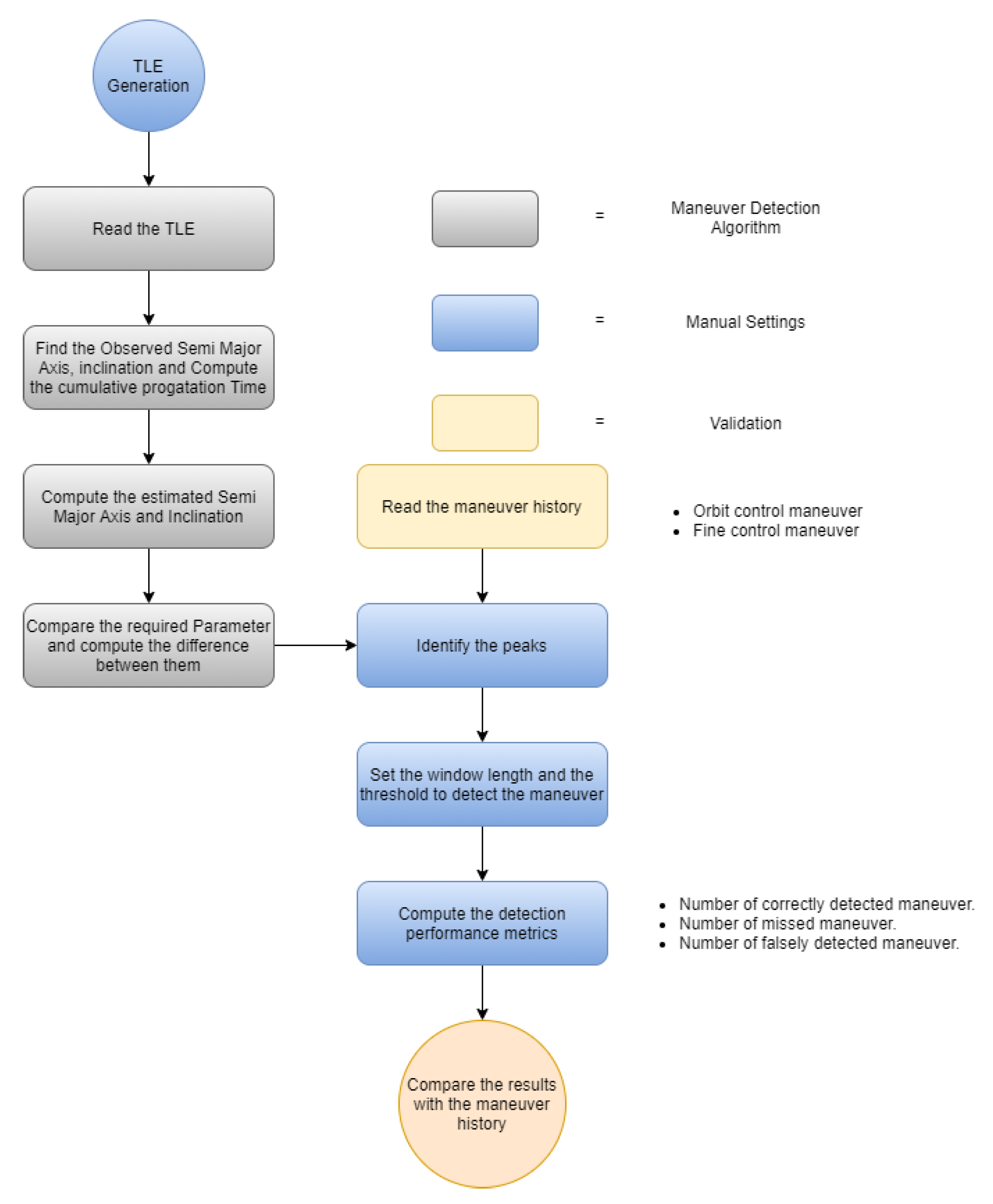
Most active satellites frequently perform only in-plane and out-of-plane maneuvers to change their semimajor axis and inclination, respectively. In-plane maneuvers are responsible for the changes that are brought about in the orbit’s shape and size by altering the semimajor axis; eventually, the orbital energy is also changed in this process. This type of maneuver evinces a sudden change in the mean motion, thereby changing orbital energy. By contrast, out-of-plane maneuvers are responsible for the changes that are brought about by the orientation of the plane by evincing an abrupt change in the inclination. In this study, an algorithm was set to detect sudden changes in the orbital parameters by calculating the difference between the adjacent segments of the orbital parameters propagated by SGP4 and the observed orbital parameters obtained from the TLEs. First, the required TLE data were downloaded from either the CelesTrak or the Space Track websites as text files [45,46]. Then, the text files were fed into the algorithm to recover the history of the satellite’s orbital parameters. Five observed orbital parameters, comprising semimajor axis, inclination, RAAN, eccentricity, and orbital energy, were extracted. In parallel, the TLE data were also fed into the SGP4 propagator to propagate the estimated orbital parameters, with the first TLE as the starting reference point; then, the parameters were propagated using SGP4 to the time the next TLE was available. The process was repeated until the last available TLE. Similarly, the five corresponding orbital parameters, comprising semimajor axis, inclination, RAAN, eccentricity, and orbital energy, were propagated. Once the two processes were completed, the observed and propagated orbital parameters were compared, and the differences between their respective values were found. Figure 1 illustrates the approach used to detect a satellite’s maneuvers.

Figure 1.
Maneuver detection and analysis algorithm.
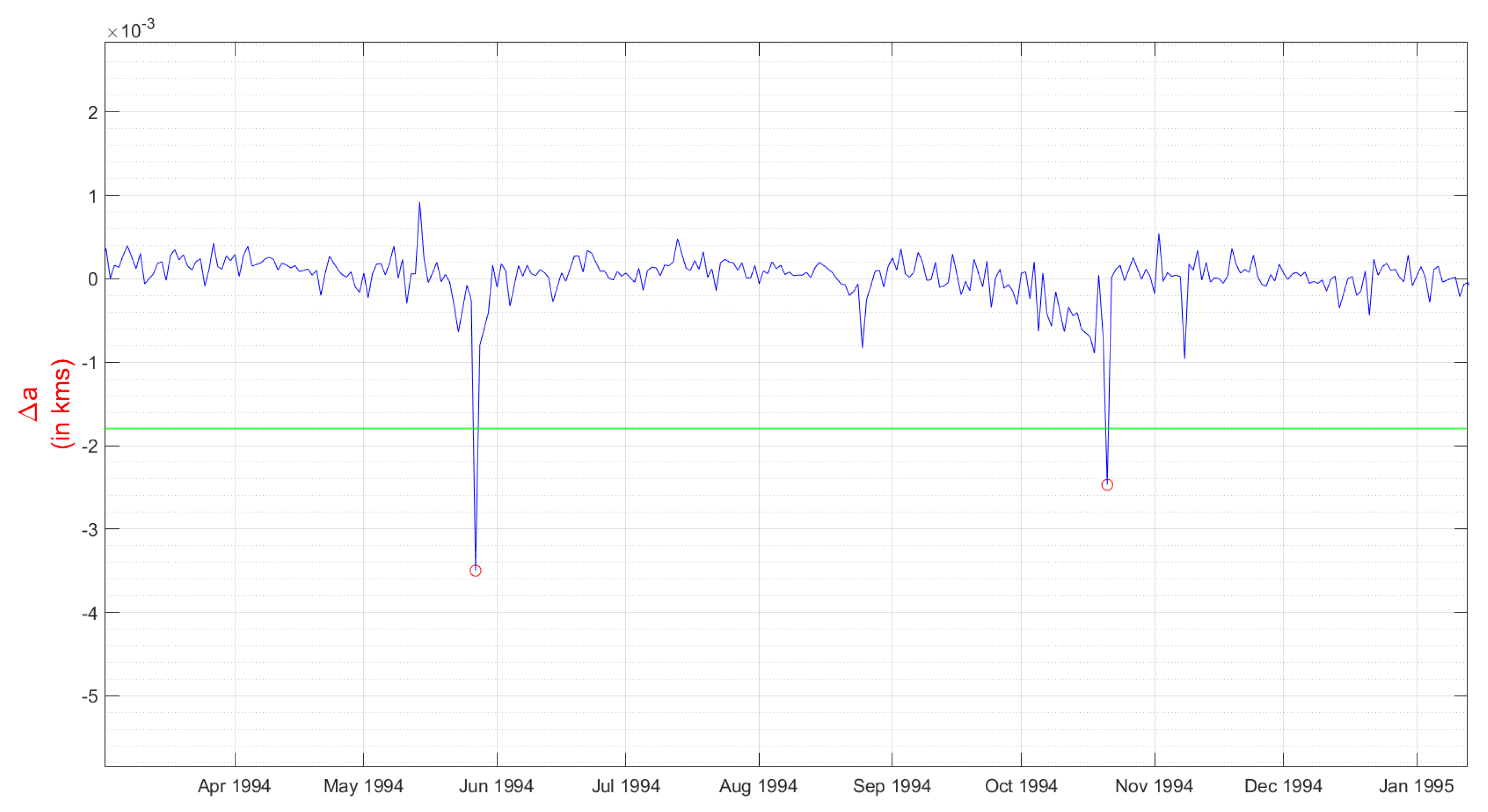
Once the differences between the corresponding propagated and observed orbital parameters were found, potential maneuvers were marked when the difference between the adjacent values exceeded a user-specified detection limit. For example, as shown in Figure 2, two potential maneuvers of TOPEX are flagged as red dots when the difference between the adjacent values exceeds a user-specified detection limit, which is represented as a horizontal green line (see Supplement Section 2 for pseudo-code used in this algorithm). The plot is a time function, which forms a peak that represents the sudden change found in the difference between the observed and propagated orbital parameters. The results of the analyses indicate that these peaks correlate with the known maneuvers of the satellite. This study follows the "trial-and-error" method in fine-tuning two parameters (i.e., window length and detection threshold) for each satellite. In this method, before finalizing the perfect values for the two parameters, the values of each parameter were manipulated to find the perfect possibilities of the two parameters that could result in perfect detection of all the maneuvers. Many factors could affect the results of this algorithm; these factors include the size of the maneuvers, the duration between each TLE data point, the time span of the data, and the gap between adjacent maneuvers. Other factors include the quality of TLE data (e.g., amount of noise in the data and skews derived from the observational and environmental effects). In consideration of the set of TLE data, the performance of the algorithm was evaluated on the basis of two parameters: window length and maneuver detection limit. Window length is the time span between each of the maneuvers, whereas detection limits are set on the basis of the peaks that represent the sudden change found in the difference between the observed and propagated orbital parameters. These parameters offer a way to judge the potentiality and sensitivity of the algorithm to detect a maneuver. This technique and the analysis may not include all discrepancies in all the environmental aspects such as gravitation, the atmosphere, vacuum, micrometeoroids, and debris, but it might be adequate to illustrate the work of the algorithm and the performance evaluation settings.
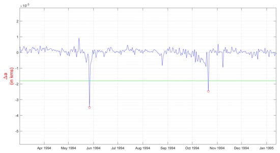
Figure 2.
Difference between the propagated and the observed semimajor axis of TOPEX. Horizontal green line is the detection limit.
3. Implementation and Results
This study focused on two satellite missions: TOPEX (SSN# 22076) (see Supplement Section 2 for the results of TOPEX) and Envisat (SSN# 27386). Both these satellites have TLE sets of high quality, and their maneuver histories are obtainable. The TLEs for both were procured from the CelesTrak website. The maneuver histories for both satellites were obtained from the International Laser Ranging Service website [46,47]. The TLE datasets and the maneuver history of both are unclassified resources and are accessible for everyone. Although the TLE data are available for almost 45,920 satellites, including decayed and in-orbit satellites, such as SES 1, NOAA 19, and GOES 13, TOPEX and Envisat were specifically chosen to represent an example of simplest fine control, in-plane maneuvers, most complex orbit control, and out-of-plane maneuvers.
3.1. Envisat
The TLE data recovered for the case study in this work cover a period of 3 years, i.e., from 2003 to 2005. The adjacent time between the TLEs averages approximately 24 h, i.e., one TLE was chosen per day to study the orbital parameters. Envisat has an average mean motion of 14 revolutions per day, with an average semimajor axis of 7152 km and an inclination of 98.5. The green vertical line in Figure 3 illustrates the known maneuver history. Envisat demonstrates a study for evaluating the performance of the algorithm, in which all green lines represent a large amplitude of out-of-plane, orbit control maneuvers with a magnitude in m/s [47]. A total of nine maneuvers performed over a period of 3 years had an average change in velocity magnitude of 1–1.5 m/s. Similar to the case study of TOPEX (see Supplement Section 2 for TOPEX case study), a baseline case was initially demonstrated and manipulated by changing the two parameters to draw an analogy between the sensitivity of the maneuver detection algorithm and the two parameters.
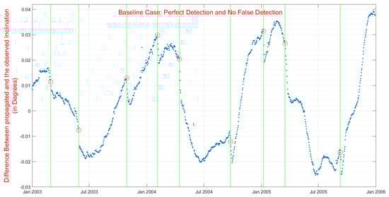
Figure 3.
Baseline case: Perfect detection and no false detection. Vertical green lines represent the maneuvers and the red circles represent potential maneuvers detected by this method.
3.1.1. Baseline Case: Perfect Detection and No False Detection
The baseline parameter is characterized by a perfect detection of all the maneuvers with no false maneuver detection. In the case study of Envisat, the baseline parameters were calibrated with a window span of 45 data points (approximately 45 days in time units) when a threshold of detection of 1-sigma was used. Figure 3 depicts the maneuvers detected as red circles. In this case, all the nine maneuvers within a period of three years were detected perfectly with no false detection.
3.1.2. Case 1: Maneuver Detection Threshold Magnified to 2-Sigma Relative to Baseline 1-Sigma Case
Figure 4 demonstrates the consequence of increasing the maneuver detection parameter to 2-sigma from 1-sigma. Given this increase, four of the nine maneuvers were undetected, whereas one false detection was noted. This result was expected because an increase in the detection threshold leads to less maneuver detection.
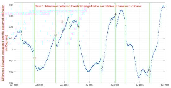
Figure 4.
Case 1: Maneuver detection threshold magnified to 2-sigma relative to baseline 1-sigma case. Vertical green lines represent the maneuvers and the red circles represent potential maneuvers detected by this method.
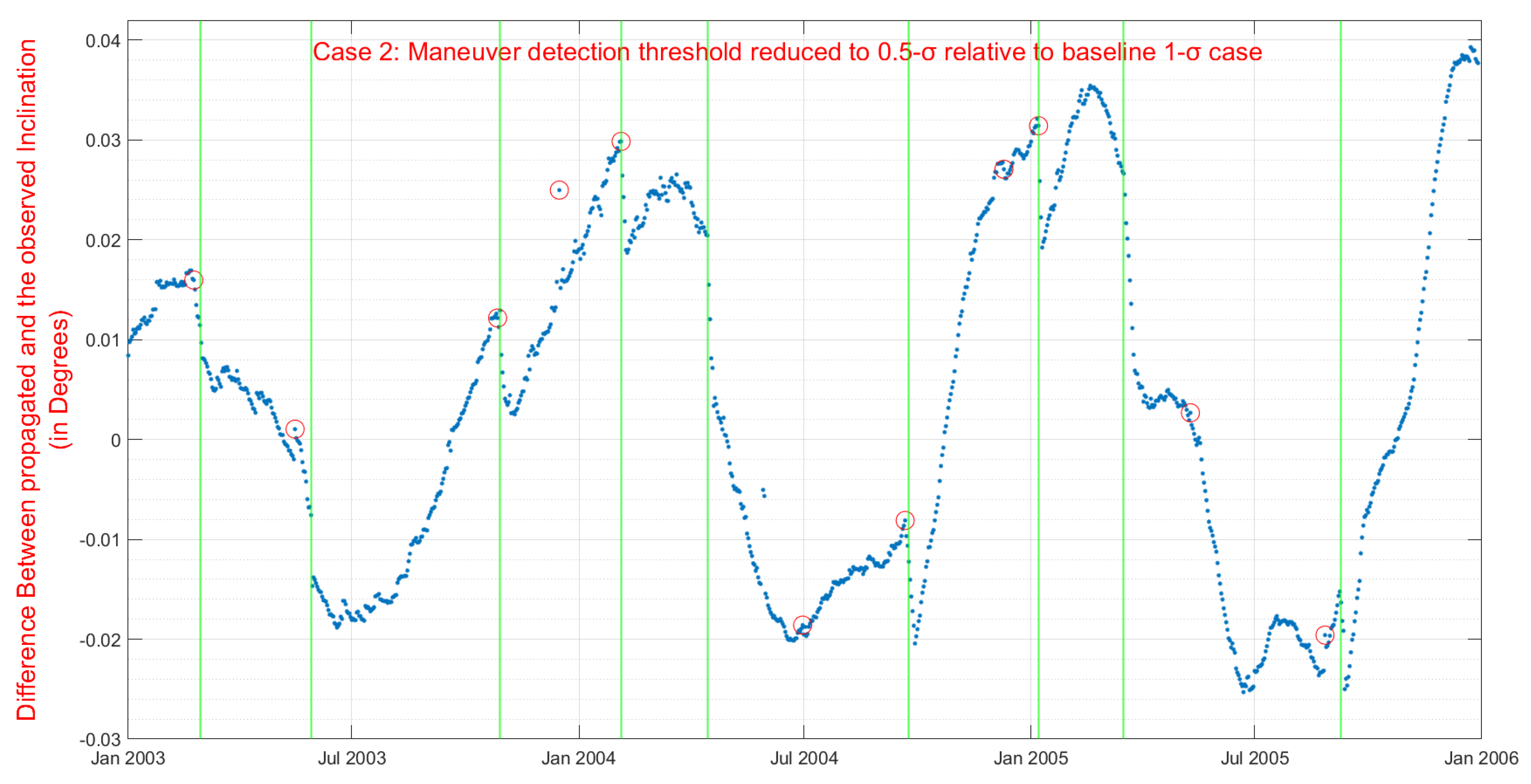
3.1.3. Case 2: Maneuver Detection Threshold Reduced to 0.5-Sigma Relative to Baseline 1-Sigma Case
Figure 5 demonstrates the consequence of decreasing the maneuver detection parameter to 0.5-sigma from 1-sigma, which resulted in the algorithm detecting five of the nine maneuvers but also six new false maneuvers. This result was also expected because decreasing the maneuver detection threshold affects the amount of false detection. Similar to the case study of TOPEX, these three cases illustrate the sensitivity between the maneuver detection threshold and maneuver detection performance.
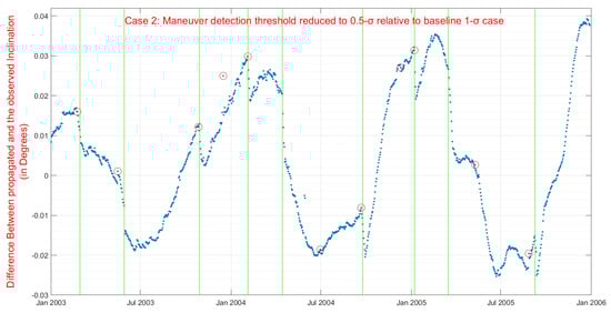
Figure 5.
Case 2: Maneuver detection threshold reduced to 0.5-sigma relative to baseline 1-sigma case. Vertical green lines represent the maneuvers and the red circles represent potential maneuvers detected by this method.
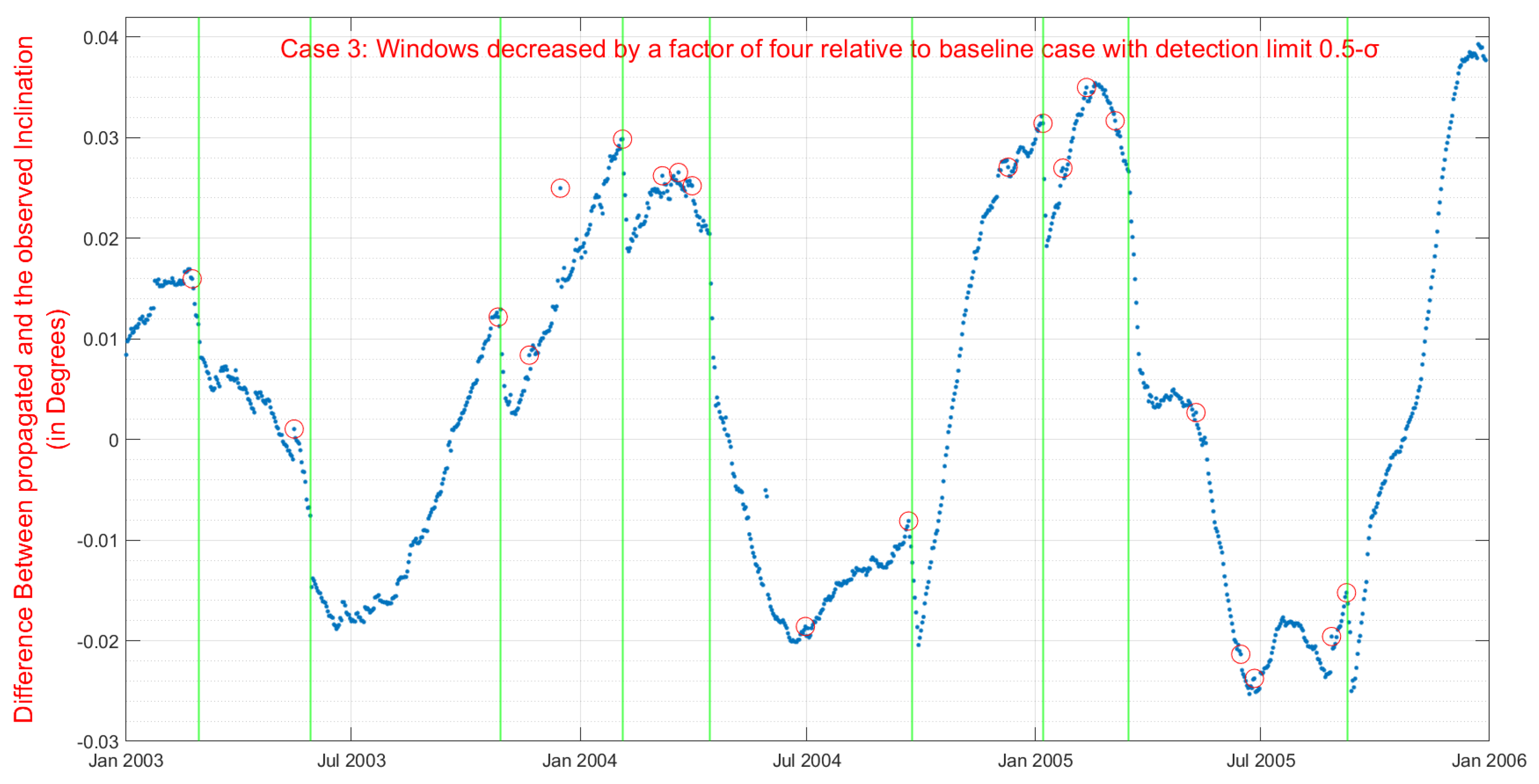
3.1.4. Case 3: Window Length Decreased by a Factor of Four Relative to Baseline Case with Detection Limit 0.5-Sigma
Figure 6 depicts the consequence of reducing the window length by a factor of four, with reference to the baseline case from 45 data points (approximately 45 days in time units) to 12 data points (approximately 12 days in time units). Given this reduction, three of the nine maneuvers, which were observed in the first case, were undetected, and 15 new false maneuvers were detected. This result is due to a decrease in the window length pushing the three cases outside of the 10-day detection threshold.

Figure 6.
Case 3: Windows decreased by a factor of four relative to baseline case with detection limit 0.5-sigma. Vertical green lines represent the maneuvers and the red circles represent potential maneuvers detected by this method.
3.1.5. Case 4: Window Increased by a Factor of Two Relative to Baseline Case with Detection Limit 0.5-Sigma
Figure 7 depicts the consequence of increasing the window length by a factor of two, with reference to the baseline case from 40 data points (approximately 40 days in time units) to 80 data points (approximately 80 days in time units). Given this increase, seven of the nine maneuvers, which were observed in the baseline case, were undetected, and four new false maneuvers were detected, resulting from the noisier data.
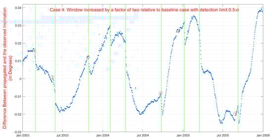
Figure 7.
Case 4: Window increased by a factor of two relative to baseline case with detection limit 0.5-sigma. Vertical green lines represent the maneuvers and the red circles represent potential maneuvers detected by this method.
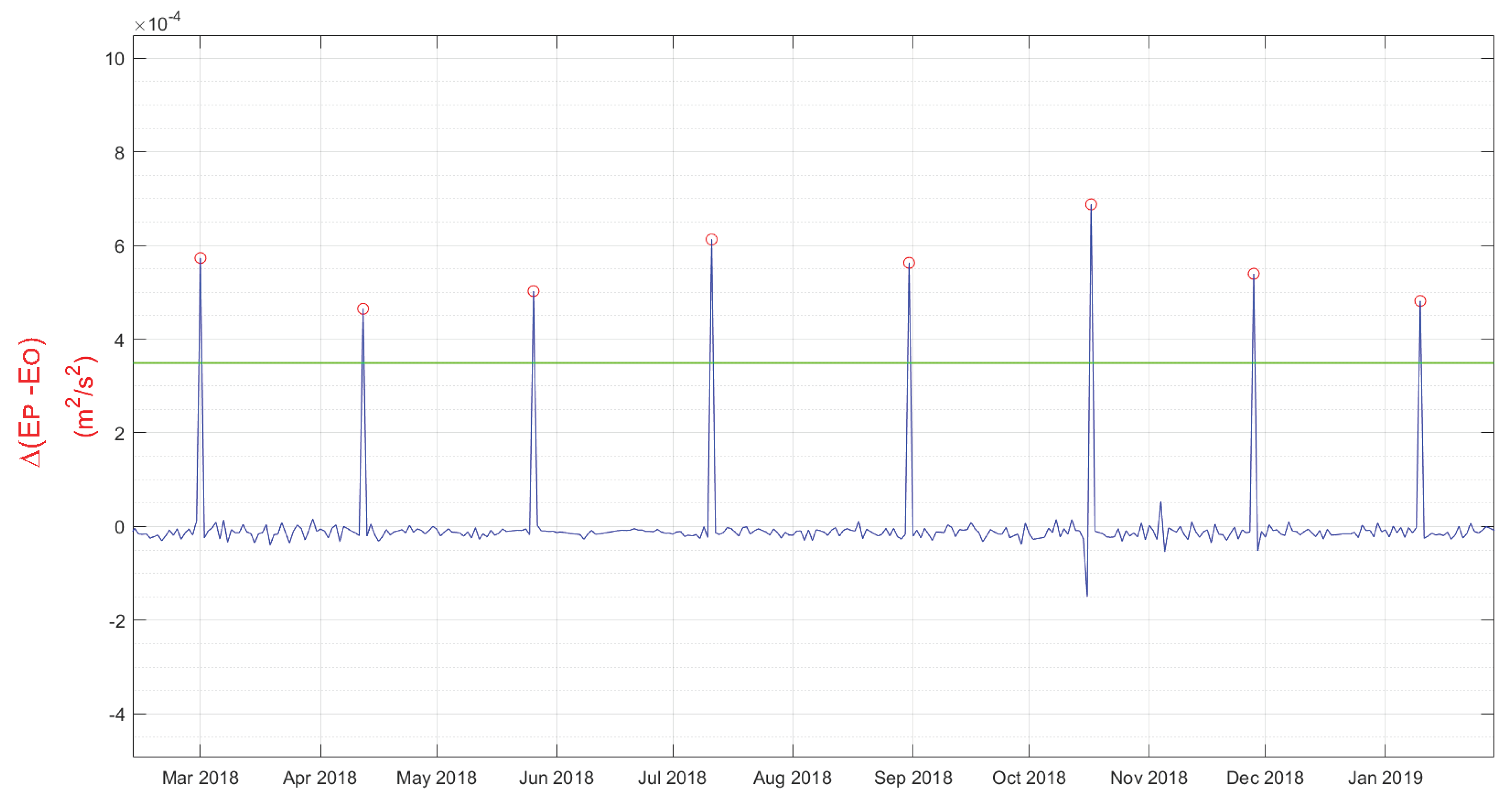
3.2. TDRS-3
The TLE data and the maneuver history of TOPEX and Envisat were studied for a period of 3 years. By analyzing the variance between the propagated semimajor axis and the observed semimajor axis, the maneuvers were detected perfectly. The same method can be applied for satellites with no available maneuver history. TDRS-3 was chosen because it has a geostationary orbit, and the TLE datasets consist of the more recent data; this scenario is different from the aforementioned two case studies. Moreover, the recent maneuver history of TDRS-3 is unknown. Satellites in geostationary orbits are perturbed by various forces, resulting in changes in inclination, longitude, and eccentricity over time. Therefore, periodic station-keeping maneuvers are executed to maintain the satellite in its assigned longitude. TDRS-3 is in a geostationary orbit, thereby allowing us to detect the orbital station-keeping maneuvers that are executed to maintain the satellite in its assigned longitude. Because of the orbit, the SDP4 propagation model is used instead of SGP4. However, the rest of the maneuver detection algorithm remains the same.
Baseline Case
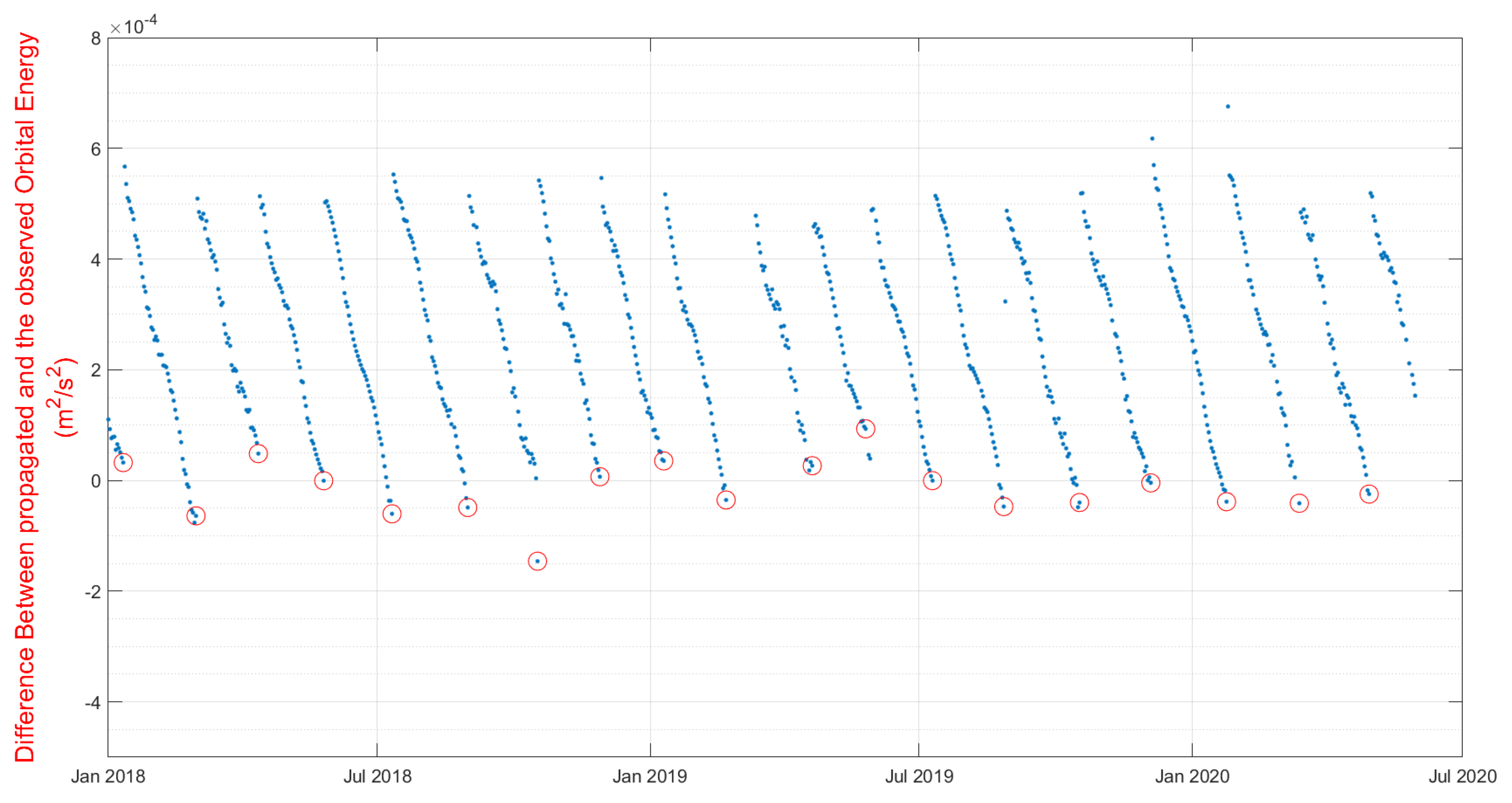
The baseline orbital parameter that is considered for the analysis is the orbital energy instead of semimajor axis because the previous two cases considered semimajor axis and inclination. However, the specific energy and semimajor axis are always the same, regardless of eccentricity. Hence, instead of using semimajor axis as a parameter to detect the maneuvers, orbital energy was used. In the implementation study of TDRS-3, the baseline parameter was calibrated with a window span of 30 data points between each maneuver detection (approximately 30 days). The analysis result of TDRS-3 consists of only the baseline case, which represents perfect detection of all the maneuvers with one false maneuver detection and is shown in Figure 8. This false detection could be due to various reasons, such as errors in particular sensors used, amount of data collected, and condition of the space environment. However, one specific reason could be an error in the TLE. Here, the difference between the propagated and the observed and the orbital energy was higher than expected. This is the reason why there was a false detection in June 2019. As shown in Figure 9, nine potential maneuvers of TDRS-3 are flagged as red dots when the difference between the adjacent values exceeds a user-specified detection limit, which is represented as a horizontal green line.
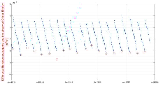
Figure 8.
Baseline Case for TDRS-3. The red circles represent potential maneuvers detected by this method.
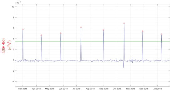
Figure 9.
TDRS-3’s difference between the propagated and the observed inclination. The horizontal green line is the detection limit; the horizontal green line represents the threshold limit and the red circles represent potential maneuvers detected by this method.
4. Discussion
Four calibrating cases have been presented in this study, thereby establishing the trade-off between the successful detection of maneuvers and the calibrating parameters of the algorithm. Detection threshold and window length are two important tuning parameters. These two parameters must be set in a manner that increases the maneuver detection reliability while reducing the occurrences of false detection. For example, reducing the detection threshold can result in an increase in the number of false detections, whereas increasing the detection threshold can result in no maneuver detection. Similarly, a reduction in the window length parameter can result in an increase in the number of false detections, whereas increasing the window length can result in no maneuver detection. Therefore, when the two parameters are selected to feed in the algorithm, the trade-off must be considered. The detection performance of the algorithm proposed in this work is relative to the data standard, number, and geometry of the maneuver. When these traits are identified clearly, the maneuver detection algorithm can be calibrated by choosing the suitable values for the two parameters, namely, detection threshold and window length, by comparing the difference between the propagated and the observed parameters. This study shows that by comparing the orbital elements obtained from TLE data and orbital elements propagated from SGP4, the maneuvers of a satellite can be predicted. The same technique can be applied to detect the maneuvers both in-plane and out-of-plane. Future work would include implementing the same method to three-satellite formation flying, which has been studied predominantly [48]. In the future the same algorithm can also be developed to detect the maneuvers in real-time by comparing the propagated Keplerian elements using SGP4 and observed Keplerian elements directly from the TLEs. Discriminating the low thrust maneuver from the other non-conservative perturbation effects could be difficult [49]. Therefore the future research should also include testing the same method with satellites in different orbits including LEOs with low thrust propulsion with different orbital parameters. This will help in detecting the maneuvers as soon as the TLEs are updated. The purpose and orbital parameters of each satellite vary and hence one set of parameters cannot be used to find the maneuvers of all the satellites. Therefore, every satellite requires different sets of threshold and window length. These two parameters must be chosen based on the spikes from the difference between the observed and the estimated parameters. For example, in Figure 9, there has been a spike every 30 days and on average the difference between the observed and the estimated orbital energy is around 4. Thus, these two values have been chosen for this case. Data preprocessing is crucial as it directly impacts the success rate of the project. Data are said to be unclean if they are missing attributes, attribute values, contain noise or outliers and duplicate or wrong data. The presence of any of these will degrade the quality of the results. However, in this study, except for the presence of a single outlier in TDRS-3, no other data-degrading factors were found and hence data preprocessing was not required. However, in the future for other case studies data preprocessing is a necessity.
5. Conclusions
Three years of TOPEX data (i.e., between 1993 and 1995) and Envisat data (i.e., between 2003 and 2005) were studied in this work, proving that the maneuvers of a satellite can be detected by analyzing the variance between the propagated semimajor axis or inclination obtained using SGP4 and the observed semimajor axis or inclination derived using TLE datasets. During this three-year period TOPEX had a total of six in-plane maneuvers while Envisat had a total of nine out-of-plane maneuvers and all the maneuvers were detected successfully. Maneuvers that are even in the range of cm/s could be detected using this technique if the parameters in the algorithm are calibrated properly. In the case studies of TOPEX and Envisat, two types of maneuvers (including fine control maneuvers, which are characterized by in-plane energy maneuvers and orbit control maneuvers, which are characterized by out-of-plane inclination maneuvers) were detected with a detection rate of 100%, even though the last part of the TOPEX data had substantial noise. Along with TOPEX and Envisat, the TLE data of TDRS-3, whose maneuver history is not available, were evaluated using the same method. A total of 19 maneuvers were performed during this period and out of the 19 maneuvers, 18 maneuvers were detected successfully. This was because of an error in the TLE data at that point. The efficiency rate of maneuver detection for TOPEX and Envisat was 100%, while for TDRS-3, which did not have any maneuver data, it was 94.73%. The data quality, density, and maneuver geometry for each satellite vary. Therefore, no one set of defined parameters could work on all satellites to detect their maneuvers under all conditions. The window length and detection threshold fed into the algorithm differ for every satellite. However, by analyzing a satellite’s semimajor axis or inclination, both the parameters can be optimized in a manner that can predict the maneuvers.
Supplementary Materials
The following are available online at https://www.mdpi.com/article/10.3390/app112110181/s1, Figure S1: Maneuver history of TOPEX, Vertical green line represents the maneuvers. Figure S2: Baseline Case, Vertical green line represents the maneuvers and the red circle represents potential maneuvers detected from this method. Figure S3: Case 1: Increase in maneuver detection threshold, Vertical green line represents the maneuvers and the red circle represents potential maneuvers detected from this method. Figure S4: Case 2: Decrease in maneuver detection threshold, Vertical green line represents the maneuvers and the red circle represents potential maneuvers detected from this method. Figure S5: Case 3: Window decreased by a factor of three relative to baseline case with detection limit 0.5-sigma, Vertical green line represents the maneuvers and the red circle represents potential maneuvers detected from this method. Figure S6: Case 4: Window increased by a factor of four relative to baseline case with detection limit 0.5-sigma, Vertical green line represents the maneuvers and the red circle represents potential maneuvers detected from this method.
Author Contributions
Conceptualization, A.M.; data curation, A.M.; formal analysis, A.M.; funding acquisition, A.M. and H.-C.W.; investigation, A.M.; methodology, A.M.; project administration, A.M. and H.-C.W.; resources, A.M.; software, A.M.; supervision, A.M. and H.-C.W.; validation, A.M.; writing—original draft, A.M.; writing—review and editing, A.M. and H.-C.W. All authors have read and agreed to the published version of the manuscript.
Funding
This research was supported by the Ministry of Science and Technology, The Republic of China, under the Grants MOST 108-2823-8-194-002, 109-2622-8-194-001-TE1, and 109-2622-8-194-007. This work was financially/partially supported by the Advanced Institute of Manufacturing with High-tech Innovations and the Center for Innovative Research on Aging Society from The Featured Areas Research Center Program within the framework of the Higher Education Sprout Project by the Ministry of Education in Taiwan.
Institutional Review Board Statement
Not applicable.
Informed Consent Statement
Not applicable.
Data Availability Statement
https://www.kaggle.com/arvindmukundan/maneuver-detection (accessed on 28 October 2021).
Conflicts of Interest
The authors declare no conflict of interest.
References
- LOSACCO, M. Orbit Determination of Resident Space Objects Using Radar Sensors in Multibeam Configuration. 2020. Available online: https://www.politesi.polimi.it/handle/10589/152295 (accessed on 28 October 2021).
- Fernandez, O.R.; Utzmann, J.; Hugentobler, U. SPOOK-A comprehensive Space Surveillance and Tracking analysis tool. Acta Astronaut. 2019, 158, 178–184. [Google Scholar] [CrossRef]
- Folcik, Z.; Cefola, P.; Abbot, R. GEO maneuver detection for space situational awareness (AAS 07-285). Adv. Astronaut. Sci. 2008, 129, 523. [Google Scholar]
- Cefola, P.J.; Weeden, B.; Levit, C. Open source software suite for space situational awareness and space object catalog work. In Proceedings of the 4th International Conference on Astrodynamics Tools Techniques, Madrid, Spain, 3–6 May 2010; pp. 3–6. [Google Scholar]
- Frueh, C. Sensor tasking for multi-sensor space object surveillance. In Proceedings of the 7th European Conference on Space Debris, Darmstadt, Germany, 18–21 April 2017; pp. 18–21. [Google Scholar]
- Moretti, N.; Rutten, M.; Bessell, T.; Morreale, B. Autonomous space object catalogue construction and upkeep using sensor control theory. In Proceedings of the Advanced Maui Optical and Space Surveillance Technologies Conf. (AMOS), Maui, HI, USA, 14–17 September 2021. [Google Scholar]
- Hobson, T.; Clarkson, I.; Bessell, T.; Rutten, M.; Gordon, N.; Moretti, N.; Morreale, B. Catalogue creation for space situational awareness with optical sensors. In Proceedings of the Advanced Maui Optical and Space Surveillance Technologies Conference, Maui, HI, USA, 20–23 September 2016. [Google Scholar]
- Kennewell, J.A.; Vo, B.N. An overview of space situational awareness. In Proceedings of the 16th International Conference on Information Fusion, Istanbul, Turkey, 9–12 July 2013; pp. 1029–1036. [Google Scholar]
- Sridharan, R.; Pensa, A.F. Us space surveillance network capabilities. In Image Intensifiers and Applications; and Characteristics and Consequences of Space Debris and Near-Earth Objects; International Society for Optics and Photonics: Bellingham, WA, USA, 1998; Volume 3434, pp. 88–100. [Google Scholar]
- Holzinger, M.J.; Scheeres, D.J.; Alfriend, K.T. Object correlation, maneuver detection, and characterization using control distance metrics. J. Guid. Control Dyn. 2012, 35, 1312–1325. [Google Scholar] [CrossRef]
- Ender, J.; Leushacke, L.; Brenner, A.; Wilden, H. Radar techniques for space situational awareness. In Proceedings of the 2011 12th International Radar Symposium (IRS), Leipzig, Germany, 7–9 September 2011; pp. 21–26. [Google Scholar]
- Patera, R.P. Space event detection method. J. Spacecr. Rockets 2008, 45, 554–559. [Google Scholar] [CrossRef]
- Huang, J.; Hu, W.; Zhang, L. Maneuver Detection of Space Object for Space Surveillance. In Proceedings of the 6th European Conference on Space Debris, Darmstadt, Germnay, 22–25 April 2013; Volume 723, p. 137. [Google Scholar]
- Oltrogge, D.L.; Alfano, S. Determination of Orbit Crosstag events and Maneuvers With Orbit Detective. In Proceedings of the AAS/AIAA Astrodynamics Specialist Conference, Girdwood, AK, USA, 31 July–4 August 2011. [Google Scholar]
- Jaunzemis, A.D.; Mathew, M.V.; Holzinger, M.J. Control cost and Mahalanobis distance binary hypothesis testing for spacecraft maneuver detection. J. Guid. Control Dyn. 2016, 39, 2058–2072. [Google Scholar] [CrossRef] [Green Version]
- Chul Ko, H.; Scheeres, D.J. Tracking maneuvering satellite using thrust-Fourier-coefficient event representation. J. Guid. Control Dyn. 2016, 39, 2554–2562. [Google Scholar] [CrossRef]
- Riesing, K. Orbit determination from two line element sets of ISS-deployed cubesats. In Proceedings of the AIAA/USU Conference on Small Satellites, Logan, UT, USA, 10–13 August 2015; pp. SSC15–x–x. [Google Scholar]
- Lemmens, S.; Krag, H. Two-line-elements-based maneuver detection methods for satellites in low earth orbit. J. Guid. Control Dyn. 2014, 37, 860–868. [Google Scholar] [CrossRef]
- Kelecy, T.; Hall, D.; Hamada, K.; Stocker, D. Satellite maneuver detection using Two-line Element (TLE) data. In Proceedings of the Advanced Maui Optical and Space Surveillance Technologies Conference, Maui Economic Development Board (MEDB), Maui, HA, USA, 12–15 September 2007. [Google Scholar]
- Li, T.; Li, K.; Chen, L. Maneuver detection method based on probability distribution fitting of the prediction error. J. Spacecr. Rockets 2019, 56, 1114–1120. [Google Scholar] [CrossRef]
- Bai, X.; Liao, C.; Pan, X.; Xu, M. Mining Two-Line Element Data to Detect Orbital Maneuver for Satellite. IEEE Access 2019, 7, 129537–129550. [Google Scholar] [CrossRef]
- Levit, C.; Marshall, W. Improved orbit predictions using two-line elements. Adv. Space Res. 2011, 47, 1107–1115. [Google Scholar] [CrossRef] [Green Version]
- Clark, R.; Lee, R. Parallel processing for orbital maneuver detection. Adv. Space Res. 2020, 66, 444–449. [Google Scholar] [CrossRef]
- Fieger, M.E. An Evaluation of Semianalytical Satellite Theory against Long Arcs of Real Data for Highly Eccentric Orbits; Technical Report; Air Force Institute of Technology: Wright-Patterson AFB, OH, USA, 1987. [Google Scholar]
- Doornbos, E.; Klinkrad, H.; Visser, P. Use of two-line element data for thermosphere neutral density model calibration. Adv. Space Res. 2008, 41, 1115–1122. [Google Scholar] [CrossRef]
- Emmert, J.; Meier, R.; Picone, J.; Lean, J.; Christensen, A. Thermospheric density 2002–2004: TIMED/GUVI dayside limb observations and satellite drag. J. Geophys. Res. Space Phys. 2006, 111. [Google Scholar] [CrossRef]
- Picone, J.; Emmert, J.; Lean, J. Thermospheric densities derived from spacecraft orbits: Accurate processing of two-line element sets. J. Geophys. Res. Space Phys. 2005, 110. [Google Scholar] [CrossRef]
- Yurasov, V.S.; Nazarenko, A.I.; Cefola, P.J.; Alfriend, K.T. Density corrections for the NRLMSIS-00 atmosphere model. Adv. Astronaut. Sci. 2005, 120, 1079–1107. [Google Scholar]
- Brouwer, D. Solution of the Problem of Artificial Satellite Theory without Drag; Technical Report; Yale University: New Haven, CT, USA, 1959. [Google Scholar]
- Lyddane, R. Small eccentricities or inclinations in the Brouwer theory of the artificial satellite. AJ 1963, 68, 555. [Google Scholar] [CrossRef]
- Aksnes, K. A second-order artificial satellite theory based on an intermediate orbit. Astron. J. 1970, 75, 1066. [Google Scholar] [CrossRef] [Green Version]
- Hoots, F.R.; Roehrich, R.L. Models for Propagation of NORAD Element Sets; Technical Report; Aerospace Defense Command Peterson AFB Co Office of Astrodynamics, 1980. [Google Scholar]
- Wei, D.; Zhao, C. Analysis on the accuracy of the SGP4/SDP4 model. Acta Astron. Sin. 2009, 50, 332–339. [Google Scholar]
- Ma, L.; Xu, X.; Pang, F. Accuracy assessment of Geostationary-Earth-Orbit with simplified perturbations models. Artif. Satell. 2016, 51, 55–59. [Google Scholar] [CrossRef] [Green Version]
- Guo, R.; Hu, X.G.; Li, X.J.; Wang, Y.; Tang, C.P.; Chang, Z.Q.; Wu, S. Application characteristics analysis of the T20 solar radiation pressure model in orbit determination for COMPASS GEO satellites. In China Satellite Navigation Conference (CSNC) 2016 Proceedings; Springer: Berlin/Heidelberg, Germany, 2016; Volume III, pp. 131–141. [Google Scholar]
- Montenbruck, O.; Steigenberger, P.; Hugentobler, U. Enhanced solar radiation pressure modeling for Galileo satellites. J. Geod. 2015, 89, 283–297. [Google Scholar] [CrossRef]
- Kerr, E.; Macdonald, M. A general perturbations method for spacecraft lifetime analysis. In Proceedings of the 25th AAS/AIAA Space Flight Mechanics Meeting, Williamsburg, VR, USA, 11–15 January 2015. [Google Scholar]
- Acquesta, E.C.; Valicka, C.G.; Hinga, M.B.; Ehn, C.B. Review of Tracktable for Satellite Maneuver Detection; Technical Report; Sandia National Laboratories (SNL-NM): Albuquerque, NM, USA, 2016. [Google Scholar]
- Mahooti, M. The SGP4 Model to Calculate Orbital State Vectors of Near-Earth Satellites. 2020. Available online: https://www.mathworks.com/matlabcentral/fileexchange/62013-sgp4 (accessed on 22 September 2021).
- Cranford, K. An improved analytical drag theory for the artificial satellite problem. In Proceedings of the Astrodynamics Conference, Princeton, NJ, USA, 20–22 August 1969; p. 925. [Google Scholar]
- Greene, M.; Zee, R. Increasing the Accuracy of Orbital Position Information from NORAD SGP4 Using Intermittent GPS Readings. 2009. Available online: https://digitalcommons.usu.edu/smallsat/2009/all2009/65/ (accessed on 28 October 2021).
- Oltrogge, D.; AGI, R.; Jens, A. Parametric Characterization of SGP4 Theory and TLE positional accuracy. In Proceedings of the Advanced Maui Optical and Space Surveillance Technologies Conference, held in Wailea, Maui, HI, USA, 9–12 September 2014. [Google Scholar]
- Dong, W.; Chang-yin, Z. An accuracy analysis of the SGP4/SDP4 model. Chin. Astron. Astrophys. 2010, 34, 69–76. [Google Scholar] [CrossRef]
- Hoots, F.R.; Roehrich, R.L.; Kelso, T. Spacetrack Report No. 3; Project Spacetrack Reports; Office of Astrodynamics, Aerospace Defense Center, ADC/DO6: Peterson AFB, CO, USA, 1980; Volume 80914, p. 14. [Google Scholar]
- Introduction and Sign in to Space-Track. Available online: https://www.space-track.org/ (accessed on 22 September 2021).
- Celestrak Homepage. Available online: http://celestrak.com/ (accessed on 22 September 2021).
- International Laser Ranging Service. Available online: https://ilrs.gsfc.nasa.gov/data_and_products/predictions/maneuver.html (accessed on 22 September 2021).
- Sabol, C.; Burns, R.; McLaughlin, C.A. Satellite formation flying design and evolution. J. Spacecr. Rockets 2001, 38, 270–278. [Google Scholar] [CrossRef]
- Kelecy, T.; Jah, M. Detection and orbit determination of a satellite executing low thrust maneuvers. Acta Astronaut. 2010, 66, 798–809. [Google Scholar] [CrossRef]


Publisher’s Note: MDPI stays neutral with regard to jurisdictional claims in published maps and institutional affiliations. |
© 2021 by the authors. Licensee MDPI, Basel, Switzerland. This article is an open access article distributed under the terms and conditions of the Creative Commons Attribution (CC BY) license (https://creativecommons.org/licenses/by/4.0/).