Measurement of the Concentration and the Brightness for Samples Containing Multiple Molecules with Different Brightness Using Fluorescence Correlation Spectroscopy

Johtaro Yamamoto; Akira Sasaki

doi:10.3390/app11135840

and

¹

Health and Medical Research Institute, National Institute of Advanced Industrial Science and Technology (AIST), Tsukuba 305-8566, Japan

²

Biomedical Research Institute, National Institute of Advanced Industrial Science and Technology (AIST), Tsukuba 305-8566, Japan

^*

Author to whom correspondence should be addressed.

Appl. Sci.2021, 11(13), 5840;https://doi.org/10.3390/app11135840

This article belongs to the Special Issue New Trends in Fluorescence Correlation Spectroscopy and Its Application Methods

Version Notes

Order Reprints

Abstract

In this study, the concentration and brightness measured by fluorescence correlation spectroscopy (FCS) in samples containing multiple species with different brightness levels was demonstrated. FCS measurements of such samples are generally difficult. However, the calculation we introduced here can provide the measurement results of the FCS. The effectiveness of the calculation was investigated based on simulations and experiments in the case of a mixture of fluorescent beads with known brightness and other fluorescent beads with unknown brightness. The results show that the concentration of the known brightness agrees well with the expected values. The obtained concentration and brightness of the species with unknown brightness is possible, and it worked well in the simulation; however, the accuracy for the species was lower than that of the species with known brightness. As a result, the calculation is useful in measuring the concentration of species with known brightness in samples containing undesired bright species, such as aggregation. The calculation for the species with unknown brightness may also be useful if good protocols or instruments are established in the future.

Keywords:

fluorescence correlation spectroscopy; fluorescence measurement; dynamics measurement

1. Introduction

Fluorescence correlation spectroscopy (FCS) is a technique that provides molecular diffusion dynamics and the number of molecules of fluorescently labeled target molecules [,,,]. The FCS system comprise a confocal fluorescence detection system. The number of target molecules inside the confocal volume (measurement volume) fluctuates owing to the translational diffusion in the sample solution. As a result, the detected fluorescence intensity signal fluctuated. This means that the fluctuation analysis of the fluorescence intensity signal can provide information about translational diffusion, which is a concept of FCS. Because FCS measurements can be performed even in living cells with low damage, FCS is a useful tool, especially in the field of biology []. For example, Sigaut et al. analyzed the mobility of a focal adhesion protein zyxin at focal adhesions of living HC11 cells by FCS. They found that the stiffness of the substrate for cell culturing did not affected to the mobility of zyxin []. A polarization dependent FCS (Pol-FCS), an advanced method of FCS, was used to evaluate the macromolecular crowding environment in cells []. Reentry, FCS is used also in the field of soft matter to evaluate the structure of materials [,].

In FCS, the speed of fluctuation of fluorescence intensity is analyzed by transforming a fluorescence intensity signal into an auto-correlation function (ACF). The characteristic decay time of the ACF, which is called the diffusion time in FCS, is inversely proportional to the diffusion coefficient of the target molecules. The amplitude of the ACF is inversely proportional to the number of molecules in the measurement volume. If a sample includes two species with different diameters, the ACF is a superposition of two ACFs with different diffusion times as described by Equation (A9) in Appendix A. If the two ACFs are separated by fitting analysis of the resulting ACF, the diffusion coefficients and the number of molecules can be obtained for each species. Therefore, FCS can be used to evaluate the molecular interactions. For example, Bhunia et al. analyzed the complex formation of enhanced green fluorescent protein (EGFP) and anti-EGFP antibodies []. Lagerkvist et al. established a phage display based on FCS. They successfully detected specific interactions between fluorescently labeled antibodies and their antigens using FCS []. Thus, FCS is useful for evaluating molecular interactions.

However, if the sample contains two species with different brightness levels, interpreting the result is difficult. The estimated number of each species becomes incorrect because their amplitude in the ACF is weighted, corresponding to the brightness of each species [,]. We can correctly obtain the number of each species only if their brightness was measured in advance. Tiwari et al. successfully measured the dimerization of green fluorescent protein-fused human glucocorticoid receptor alpha (GFP-GRα) using FCS. They assumed that there were only monomers and dimers of GFP-GRα, and the brightness of dimers was two times larger than that of the monomer. In addition, the brightness of the GFP-GRα monomer was measured as a negative control before the sample measurement []. There are similar approaches for the dimer and oligomer formation analysis [,,,]. Katoozi et al. proposed the high-order image correlation spectroscopy (HICS) which is based on high-order ACF analysis []. They successfully evaluate the numbers of each species and the brightness ratio between multiple species without any assumption. This approach may be useful for FCS too. However, most of the available FCS instruments and hardware correlators do not provide high-order autocorrelation function so far. Introducing high-order ACF is difficult for current FCS users.

The brightness of a target molecule is characterized by the photon count rate per molecule, which is called the count per molecule (CPM), because the fluorescence intensity is measured by a photon counting method in FCS. The CPM of the second species is often unknown in applications, such as multimer, aggregation, antigen, and antibody response of one-to-many association. Methods to analyze the ACF of FCS correctly in the case of samples containing multiple brightness species are strongly desired in FCS.

In this report, we introduced a calculation procedure for FCS analysis for samples containing multiple brightness species. This calculation can be applied if the diffusion time of each species is obtained separately, and the brightness of M-1 species in M species is determined before measurement. Furthermore, the calculation requires only the first order ACF, which is provided by general FCS instruments, and its fitting results are based on the common model equation. We describe the simulation results of the calculation and its experimental demonstration.

2. Materials and Methods

2.1. Monte Carlo Simulation of Fluorescence Intensity Signal in FCS Measurement

To validate our correction method for a number of molecules and CPM in the FCS, a Monte Carlo simulation was performed. Fluorescence intensity signals from a sample solution containing two species with different CPMs were generated. The details of this simulation are provided in Appendix B.

Ten fluorescence intensity signals with a duration of 10 s and a time interval of 1 ms were generated. The lateral radius of the confocal volume was

w_{0} = 250

nm, and the axial radius was

z_{0} = 1250

nm. The measurement volume of the FCS, which is called the effective measurement volume, was

4.35 \times 10^{- 19}

m³ (0.435 fL). The diameters of the first and second species were 10 and 100 nm, respectively. The medium was water with a viscosity of 0.89 cP, and the absolute temperature was 300 K. In this case, the diffusion coefficient of the first species was 49.4 μm²/s, and the typical step length in Equations (A22)–(A24) (the square root of the mean square displacement) was

\sqrt{2 D Δ t} = 314.2

nm. This was shorter than the lateral diameter of the confocal volume, however it was not enough short to correctly analyze the diffusion time. However, the amplitudes of the ACF, which is focused on in this work, can be correctly obtained because that is given by only the variance and the average of fluorescence intensity signal as obtained by substituting

τ = 0

for Equation (A5) in the case that the shot noise can be negligible.

2.2. Number of Molecules Calculation

It is assumed that there are two species: fluorescently labeled small molecules and larger particles containing multiple fluorescent dyes, such as aggregates. If the CPM of the first species

ε_{1}

can be determined by FCS measurement on a pure solution in advance, the number of the first species

n_{1}

can be estimated by applying the proposed calculation. The CPM of the second species

ε_{2}

and the number

n_{2}

were also estimated by further correction. The details of the correction method are provided in Appendix A.

2.3. FCS Measurement

Model experiments were performed to experimentally demonstrate the proposed correction method. The FCS measurements were performed on mixtures of two fluorescent latex beads, a fluorescent bead with a diameter of 30 nm (PSYF030NM, MAGSPHERE, Pasadena, CA, USA), and a brighter bead with a diameter of 51 nm (PSYF050NM, MAGSPHERE, Pasadena, CA, USA). A compact FCS system (307-15471, Wako, Japan) was used for the measurements. The lateral diameter of the confocal volume was 200.3 nm, and the axial diameter was 1.14 μm. The effective measurement volume was determined to be 0.255 fL. The excitation wavelength was 473 nm. The excitation laser power was 0.5 μW at the focal point. The 3 s measurement was repeated 20 times, and one mean ACF was obtained. The non-linear least squares analysis was performed on the mean ACF for one experiment.

3. Results

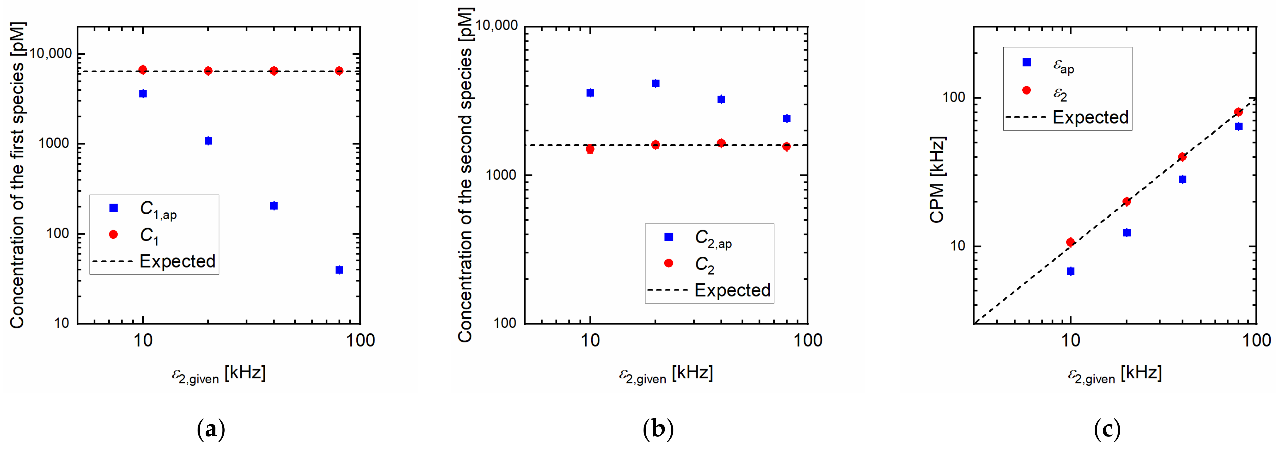
Figure 1 shows the dependency of the estimated parameters on the concentration of the second species in the Monte Carlo simulation. The CPMs of the first and second species were 5 and 100 kHz, respectively. We assumed that the CPM and the diffusion time of the first species were determined by measuring the pure solution of the first species, and we can correctly separate the fractions of the first and second species in the obtained ACF. The number and CPM of the second species were unknown. The concentration of the first species was 6400 pM, and the second species was the dilution series in the generation of the fluorescence signal by simulation described in Appendix B. Figure 1a shows a comparison of the estimated concentration of the first species

C_{1}

and the given concentration of the second species

C_{2, given}

. The apparent concentration

C_{1, ap}

, which was obtained using Equation (A11), of the first species decreased with an increase in the

C_{2, given}

despite the concentration of the first species being independent of the concentration of the second species. Note that the apparent concentration obtained by Equation (A11) is not correct value and should not be used in the case of the samples containing multiple brightness species because the apparent value is theoretically incorrect and the discrepancy between the apparent values and the expected value can be large as shown in the Figure 1. Conversely, the concentration of the first species obtained by Equations (A14) and (A21)

C_{1}

was independent of the

C_{2, given}

, and the values agreed well with the expected value. Figure 2a shows a comparison between the estimated

C_{2}

and the given

C_{2, given}

. The error of the apparent concentration of the second species

C_{2, ap}

was large, especially at low concentrations of brighter species; however, the concentration obtained by our calculation

C_{2}

was in good agreement with the expected concentration. Figure 1c shows the results of the CPM. The apparent CPM is given by Equation (A12) in Appendix A. The apparent CPM increased with the increase in the number of brighter species and approached the given CPM of the second species. In contrast, the corrected CPM was in good agreement with the given CPM of the second species.

Figure 1. Dependency of the given concentration of the second species. (a) Dependency on the measured concentration of the first species

C_{1}

; (b) dependency on the measured concentration of the second species

C_{2}

; (c) dependency on the measured CPM. Error bars show the standard errors (

n = 10

).

Figure 2. Dependency of the given CPM of the second species

ε_{2, given}

. (a) Dependency on the measured concentration of the first species

C_{1}

; (b) dependency on the measured concentration of the second species

C_{2}

; (c) dependency on the measured CPM. Error bars show the standard errors (

n = 10

).

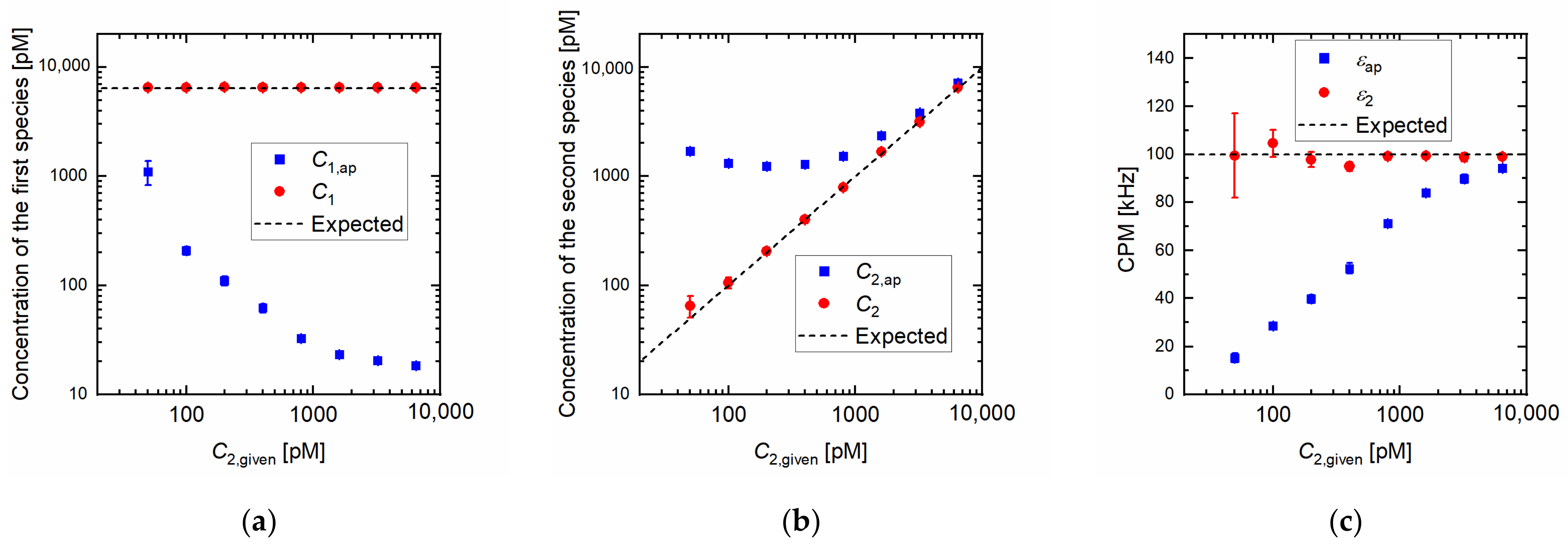
Figure 2 shows the dependency of the estimated parameters on the CPM of the second species

ε_{2}

in the Monte Carlo simulation. The given

C_{1}

and

C_{2}

were fixed at 6400 and 1600 pM, respectively. The given CPM of the first species

ε_{1, given}

was fixed at 5 kHz. The error of

C_{1, ap}

became larger with the increase in the given

ε_{2, given}

, and the error of

C_{2, ap}

became smaller, as shown in Figure 2a,b. The apparent CPM

ε_{ap}

was always underestimated, as shown in Figure 2c.

In contrast, the values obtained by the calculation we proposed are in good agreement with the expected values.

Finally, we applied the correction method to the experimental results. Figure 3 shows the results of FCS measurement on the mixture of two fluorescent beads: Beads1 with a diameter of 30 nm and Beads2 with a diameter of 51 nm. The CPM of Beads1 and Beads2 were measured as

6.82 \pm 0.02

and

26.5 \pm 0.2

kHz, respectively, in pure solutions. The number of Beads1 was fixed at 57.9 (final concentration), and the dilution series of Beads2 was mixed into the Beads1 solution. In the fitting analysis of the obtained ACFs, the model Equation (A9) was used for two species. The diffusion time of the first species was fixed to the value measured in pure solutions to improve the accuracy of the fitting because we assumed that the first species was known. The measurements were performed four times on the same samples, but at different positions in the solution (

n = 8

). The numbers of the first species

{\bar{n}}_{1}

obtained by Equation (A14) agreed well with the expected values, as shown in Figure 3a. The numbers of the second species

{\bar{n}}_{2}

obtained by Equation (A17), also agreed with the expected values in the range of dilution ratio of Beads2 was higher than 0.1 as shown in Figure 3b. In the range of dilution ratio of Beads2 lower than 0.1, the error of

{\bar{n}}_{2}

was large. This was likely caused by too low concentration of the Beads2. Figure 3c shows the apparent CPM

ε_{ap}

and the corrected CPM₂

ε_{2}

. In the high concentration range of Beads2, some data points took the values around the expected value. There were also the data points with

ε_{2}

higher than the expected value. This was likely indicating that there was some small aggregation of fluorescent beads. The data points of

ε_{2}

were decreased from n=8 because the corrected

{\bar{n}}_{2}

was 0 at some data points, and we could not calculate

ε_{2}

because of division by zero in that case.

Figure 3. Dependency of the given CPM of the second species. (a) Dependency on the measured concentration of the first species

C_{1}

. (b) Dependency on the measured concentration of the second species

C_{2}

. Only the error bars in positive direction are shown. (c) Dependency on the measured CPM. Black broken lines show the expected values. Error bars show the standard errors (

n = 8

).

4. Discussion

We investigated the dependency of the estimated parameters on the concentration of the second species (Figure 1). The CPMs of the first and second species,

ε_{1}

and

ε_{2}

, were 5 and 100 kHz, respectively. It was assumed that the first species is known and had been measured by FCS in pure solution in advance, and the second species is its aggregation or molecules labeled by multiple first species. Therefore, the concentration of the second species

C_{2}

was lower than that of the first species

C_{1}

, and

ε_{2} > ε_{1}

in the simulations. The results demonstrate the effectiveness of the proposed correction method. Figure 1a shows that the apparent

C_{1, a p}

can be underestimated by one order even if the

C_{2}

is two orders lower than

C_{1}

in the simulation condition. Figure 1b,c show that the concentration and CPM of brighter species are likely to be measured without our calculation if the concentration of the brighter species is sufficiently high because, in that case, the contribution of the brighter species in fluorescence intensity becomes much larger than that of the first species. The deviation of the

ε_{2}

is relatively large. This is likely because the error in the estimation of

ε_{2}

is enhanced as the

ε_{2}

was estimated based on the estimated value of

ε_{1}

.

The dependency of the estimated parameters on the given CPM of the second species

ε_{2}

is also shown in Figure 2. It was shown that the error of

C_{1}

became larger with the increase in

ε_{2}

. Thus, the FCS results can be easily distorted by contamination of the brighter species in the samples.

In the experiment on the mix of two fluorescent bead solutions with different brightness, the calculation of

{\bar{n}}_{1}

worked well; however, the accuracies of the calculation on

{\bar{n}}_{2}

and

ε_{2}

were lower than those on the

{\bar{n}}_{1}

. This was likely caused by the estimation of

{\bar{n}}_{2}

and

ε_{2}

based on the estimated value of

ε_{1}

as shown in Appendix A. To obtain accurate values of

{\bar{n}}_{2}

and

ε_{2}

, the measurement should be performed carefully and accurately. Small differences in particle brightness owing to hardware conditions, such as laser power fluctuation and/or changing fluorescence collection efficiency by changing the light path during the measurement can deviate the corrected values.

5. Conclusions

In this work, we proposed a calculation procedure for the concentration (number of molecules/effective measurement volume) and brightness (CPM) in FCS measurements on samples containing multiple species with different CPMs. From the simulations, it was shown that the presence of the second species with a higher CPM than the first species can distort the results of FCS.

If all CPMs of every species in a sample are known, we can correctly analyze the number of molecules in each species []. On the other hand, the proposed calculation procedure can be applied if the CPM of only the first species is known, and the fraction of each species can be accurately separated by fitting the analysis of FCS. It was shown that the proposed calculation worked well by the simulations and the experiments.

Theoretically, this calculation can be expanded to include more species. However, it may not be applicable practically because an increase in the species should degrade the accuracy.

We expect that accurate measurement of the mixtures, for example, the sample containing the monomer and its aggregation or its oligomer, and the sample containing the free fluorescent antibody and the particles associated with multiple antibodies, will be available using FCS and our calculation procedure.

Author Contributions

Conceptualization, J.Y.; Methodology, J.Y.; Software, J.Y.; Validation, J.Y. and A.S.; Formal Analysis, J.Y.; Investigation, J.Y. and A.S.; Resources, A.S.; data curation, J.Y.; writing—original draft preparation, J.Y.; writing—review and editing, J.Y.; visualization, J.Y.; supervision, J.Y.; project administration, J.Y.; funding acquisition, J.Y. All authors have read and agreed to the published version of the manuscript.

Funding

This research was funded by the Japan Society for the Promotion of Science (JSPS), grant number 19K06591.

Conflicts of Interest

The authors declare no conflict of interest.

Appendix A

We assume that there are M species in the sample solution, and the fluorescence intensity emitted from the m-th species can be expressed as:

I_{m} (t) = δ I_{m} (t) + {\bar{I}}_{m},

(A1)

δ I_{m} (t) = ε_{m} δ n_{m} (t),

(A2)

{\bar{I}}_{m} = ε_{m} {\bar{n}}_{m},

(A3)

where the subscript m denotes the m-th species.

δ I

and

\bar{I}

denote the fluctuation component and the mean fluorescence intensity, respectively.

ε

denotes the brightness per molecule, which is called the CPM.

δ n

and

\bar{n}

are the fluctuation component and mean value of the number of molecules inside the confocal volume of the FCS, respectively. Therefore, the total fluorescence intensity is

I (t) = \sum_{m = 1}^{M} I_{m} (t) .

(A4)

The ACF of FCS is expressed as follows []:

G (τ) = \frac{I (t) \cdot I (t + τ)}{{\bar{I}}^{2}} = 1 + \frac{⟨ δ I (t) \cdot δ I (t + τ) ⟩}{{\bar{I}}^{2}},

(A5)

= 1 + \sum_{m = 1}^{M} \frac{ε_{m}^{2} {\bar{n}}_{m}}{{\bar{I}}^{2}} G_{m} (τ),

(A6)

A_{m} = \frac{ε_{m}^{2} {\bar{n}}_{m}}{{\bar{I}}^{2}},

(A7)

where

A_{m}

denotes the amplitude of the ACF for the m-th species.

G_{m}

denotes the decaying ACF with an amplitude of unity. The angle brackets ⟨ ⟩ represent the ensemble average. For three-dimensional (3D) free diffusion,

G_{m}

can be expressed as follows []:

G_{m} (τ) = {(1 + \frac{τ}{τ_{D, m}})}^{- 1} {(1 + \frac{1}{s^{2}} \frac{τ}{τ_{D, m}})}^{- \frac{1}{2}},

(A8)

where

τ_{D, m}

denotes the diffusion time of the m-th species.

In FCS measurements, the experimentally obtained ACFs are fitted by the following 3D diffusion model equation based on the non-linear least squares:

G (τ) = 1 + \frac{1}{N_{ap}} \sum_{m = 1}^{M} F_{ap, m} G_{m} (τ),

(A9)

\sum_{m = 1}^{M} F_{a p, m} = 1,

(A10)

where

N_{ap}

denotes the apparent total number of all the species and

F_{ap, m}

denotes the apparent fraction of the m-th species. If the CPM of each species is the same,

N_{ap}

and

F_{a p, m}

are equal to their true values. The apparent number of m-th species is given by

N_{a p, m} = F_{a p, m} N_{a p} .

(A11)

The apparent CPM is defined by

ε_{a p} = \frac{\bar{I}}{N_{a p}} .

(A12)

Note that the apparent values

ε_{a p}

,

N_{ap}

, and

F_{ap, m}

are incorrect if the sample contain multiple species with different brightness and should not be used. However, those can be easily obtained by most of available FCS instruments and their software using the most common model equation in FCS shown in Equation (A9). The calculation procedure to obtain correct values from such the apparent values is useful to most of FCS users. We introduce here the procedure.

For simplicity, we assumed that there are two species, a fluorescently labeled monomer protein and its aggregates, and that the CPM of the monomer protein can be measured by a purified sample. The ACF obtained by an FCS measurement on the sample containing a second species with unknown CPM is fitted by Equation (A9), and N_ap and F_ap are obtained. Using Equations (A7) and (A9), the amplitude of the ACF owing to the monomer protein is:

\frac{ε_{1}^{2} {\bar{n}}_{1}}{{\bar{I}}^{2}} = \frac{F_{a p, 1}}{N_{ap}} .

(A13)

Subsequently, the true number of first species can be obtained as follows:

{\bar{n}}_{1} = \frac{F_{a p, 1}}{N_{ap}} \frac{{\bar{I}}^{2}}{ε_{1}^{2}} .

(A14)

Multiplying the amplitude of the second species by the ratio

{\bar{I}}^{2} / {\bar{I}}_{2}^{2}

,

\frac{{\bar{I}}^{2}}{{\bar{I}}_{2}^{2}} A_{2} = \frac{{\bar{I}}^{2}}{{\bar{I}}_{2}^{2}} \frac{ε_{2}^{2} {\bar{n}}_{2}}{{\bar{I}}^{2}} = \frac{ε_{2}^{2} {\bar{n}}_{2}}{{\bar{I}}_{2}^{2}},

(A15)

= \frac{ε_{2}^{2} {\bar{n}}_{2}}{ε_{2}^{2} {\bar{n}}_{2}^{2}} = \frac{1}{{\bar{n}}_{2}} .

(A16)

Using Equations (A3), (A4), (A12), and (A14), the number of the second species can be obtained as follows:

{\bar{n}}_{2} = {(\frac{{\bar{I}}_{2}}{\bar{I}})}^{2} \frac{N_{ap}}{F_{a p, 2}} = {(\frac{\bar{I} - ε_{1} {\bar{n}}_{1}}{\bar{I}})}^{2} \frac{N_{ap}}{F_{a p, 2}} .

(A17)

The CPM of second species can be obtained as follows:

ε_{2} = \frac{{\bar{I}}_{2}}{{\bar{n}}_{2}} = \frac{\bar{I} - ε_{1} {\bar{n}}_{1}}{{\bar{n}}_{2}} .

(A18)

If

{\bar{I}}_{2} < 0

, we assumed

{\bar{n}}_{2} = 0

because we can assume that there were few or no second species in the measurement duration in that case.

Similarly, if the CPMs of the M-1 species in M species are known, the number of molecules and CPM of each species can be corrected in the same way.

Appendix B

To confirm the proposed calculation, a Monte Carlo simulation was performed. Fluorescence intensity fluctuations detected by confocal fluorescence detection in fluorescence solutions were generated. The point spread function (PSF) of the confocal system is defined as follows []:

W (x, y, z) = \exp [- 2 \frac{x^{2} + y^{2}}{w_{0}^{2}} - 2 \frac{z^{2}}{z_{0}^{2}}],

(A19)

where

w_{0}

and

z_{0}

denote the lateral radius and axial radius of the confocal volume, respectively. The z-axis represents the optical axis of the system. The effective measurement volume

V_{eff}

of the FCS measurement [] is defined as

V_{eff} = π^{\frac{3}{2}} w_{0}^{2} z_{0} .

(A20)

The cuboid volume of interest in the simulation was defined as

- L_{x} / 2 \leq x \leq L_{x} / 2

,

- L_{y} / 2 \leq y \leq L_{y} / 2

, and

- L_{z} / 2 \leq z \leq L_{z} / 2

. The widths in

x

- and

y

-axis are

L_{x}

and

L_{y}

, respectively. The height was

L_{z}

. In this case, the number of molecules in the volume of interest

N_{0}

is

N_{0} = C N_{A} \times 1000 V_{eff},

(A21)

where

C

denotes the molar concentration of the target molecules.

In this simulation, the positions of each of

N_{0}

molecules were randomly determined, and the fluorescence intensity to be detected was calculated using the position and the PSF. The position of the

i

-th molecule (

x_{i}

,

y_{i}

,

z_{i}

) at time point

n

is calculated as follows:

x_{i, n + 1} = x_{i, n} + R_{N} (0, \sqrt{2 D Δ t}),

(A22)

y_{i, n + 1} = y_{i, n} + R_{N} (0, \sqrt{2 D Δ t}),

(A23)

z_{i, n + 1} = z_{i, n} + R_{N} (0, \sqrt{2 D Δ t}),

(A24)

where

R_{N} (0, \sqrt{2 D Δ t})

represents a random number obeying a normal distribution with a mean of 0 and a standard deviation of

\sqrt{2 D Δ t}

.

D

denotes the diffusion coefficient of the target molecules, and

Δ t

is the time interval of the simulation. The initial positions of the molecules were determined by uniform random numbers within the volume of interest. If a molecule exits to the outside of the volume, the molecule enters from the opposite of the volume.

The fluorescence intensity to be detected at the

n

-th time point can be calculated as

I_{n} = \sum_{i = 1}^{N_{0}} I_{i, n},

(A25)

I_{i, n} = ε_{0} W (x_{i, n}, y_{i, n}, z_{i, n}),

(A26)

where

I_{i, n}

is the fluorescence intensity of the

i

-th molecule.

ε_{0}

denotes the brightness of the target molecule at the origin (the focal point of the system). The brightness obtained by the FCS measurement (CPM)

ε

is

ε = γ ε_{0},

(A27)

γ = \frac{\int \int \int {[W (x, y, z)]}^{2} d x d y d z}{\int \int \int W (x, y, z) d x d y d z},

(A28)

where

γ = \sqrt{2} / 4

for the 3D gaussian PSF defined by Equation (A19).

If there are two or more species with different brightness levels, the fluorescence intensity for each species is superimposed.

We calculated the apparent parameters and the corrected parameters from the FCS analysis of the generated fluorescence intensity based on the method described in Appendix A. Finally, the results and the given parameters were compared.

References

Elson, E.L.; Magde, D. Fluorescence correlation spectroscopy. I. Conceptual basis and theory. Biopolymers 1974, 13, 1–27. [Google Scholar] [CrossRef]
Aragón, S.R.; Pecora, R. Fluorescence correlation spectroscopy as a probe of molecular dynamics. J. Chem. Phys. 1976, 64, 1791–1803. [Google Scholar] [CrossRef]
Rigler, R.; Mets, Ü.; Widengren, J.; Kask, P. Fluorescence correlation spectroscopy with high count rate and low background: Analysis of translational diffusion. Eur. Biophys. J. 1993, 22, 169–175. [Google Scholar] [CrossRef]
Elson, E.L. Introduction to fluorescence correlation Spectroscopy—Brief and simple. Methods 2018, 140–141, 3–9. [Google Scholar] [CrossRef] [PubMed]
Hess, S.T.; Huang, S.; Heikal, A.A.; Webb, W.W. Biological and chemical applications of fluorescence correlation spectroscopy: A review. Biochemistry 2002, 41, 697–705. [Google Scholar] [CrossRef] [PubMed]
Sigaut, L.; Bianchi, M.; von Bilderling, C.; Pietrasanta, L.I. Correlation of cellular trancition forces and dissociation kinetics of adhesive protein zyxin revealed by multi-parametric live cell microscopy. PLoS ONE 2021, 16, e0251411. [Google Scholar] [CrossRef] [PubMed]
Yamamoto, J.; Matsui, A.; Gan, F.; Oura, M.; Ando, R.; Matsuda, T.; Gong, J.P.; Kinjo, M. Quantitative evaluation of macromolecular crowding environment based on translational and rotational diffusion using polarization dependent fluorescence correlation spectroscopy. Sci. Rep. 2021, 11, 10594. [Google Scholar] [CrossRef] [PubMed]
Gupta, A.; Sankaran, J.; Wohland, T. Fluorescence correlation spectroscopy: The technique and its applications in soft matter. Phys. Sci. Rev. 2019, 4, 20170104. [Google Scholar] [CrossRef]
Bhunia, D.; Chowdhury, R.; Bhattacharyya, K.; Ghosh, S. Fluorescence fluctuation of an antigen–antibody complex: Circular dichroism, FCS and smFRET of enhanced GFP and its antibody. Phys. Chem. Chem. Phys. 2015, 17, 25250–25259. [Google Scholar] [CrossRef] [PubMed]
Lagerkvist, A.C.; Földes-Papp, Z.; Persson, M.A.A.; Rigler, R. Fluorescence correlation spectroscopy as a method for assessment of interactions between phage displaying antibodies and soluble antigen. Protein Sci. 2001, 10, 1522–1528. [Google Scholar] [CrossRef] [PubMed]
Lakowicz, J.R. Fluorescence correlation spectroscopy. In Principles of Fluorescence Spectroscopy; Springer US: Boston, MA, USA, 2006; pp. 797–840. [Google Scholar]
Tiwari, M.; Oasa, S.; Yamamoto, J.; Mikuni, S.; Kinjo, M. A Quantitative study of internal and external interactions of homodimeric glucocorticoid receptor using fluorescence cross-correlation spectroscopy in a live cell. Sci. Rep. 2017, 7, 4336. [Google Scholar] [CrossRef] [PubMed] [Green Version]
Rauer, B.; Neumann, E.; Widengren, J.; Rigler, R. Fluorescence correlation spectrometry of the interaction kinetics of tetramethylrhodamin alpha-bungarotoxin with Torpedo californica acetylcholine receptor. Phys. Chem. 1996, 58, 3–12. [Google Scholar] [CrossRef]
Kaliszewski, M.J.; Shi, X.; Hou, Y.; Lingerak, R.; Kim, S.; Mallory, P.; Smith, A.W. Quantifying membrane protein oligomerization with fluorescence cross-correlation spectroscopy. Methods 2018, 140–141, 40–51. [Google Scholar] [CrossRef] [PubMed]
Paul, M.D.; Rainwater, R.; Zuo, Y.; Gu, L.; Hristova, K. Probing membrane protein association using concentration-dependent number and brightness. Angewandte Chem. Int. Ed. 2021, 60, 6503–6508. [Google Scholar] [CrossRef]
Melo, A.M.; Prieto, M.; Coutinho, A. Quantifying lipid-protein interaction by fluorescence correlation spectroscopy (FCS). In Fluorescence Spectroscopy and Microscopy. Methods in Molecular Biology (Methods and Protocols), 2nd ed.; Engelborghs, Y., Visser, A., Eds.; Humana Press: Totowa, NJ, USA, 2014; Volume 1076, pp. 575–595. [Google Scholar]
Katoozi, D.; Clayton, A.H.A.; Moss, D.J.; Chon, J.W.M. Uptake quantification of gold nanoparticles inside of cancer cells using high order image correlation spectroscopy. Biomed. Opt. Express 2021, 12, 539–552. [Google Scholar] [CrossRef]
Schwille, P. Fluorescence correlation spectroscopy and its potential for intracellular applications. Cell Biochem. Biophys. 2001, 34, 383–408. [Google Scholar] [CrossRef]

Figure 1. Dependency of the given concentration of the second species. (a) Dependency on the measured concentration of the first species

C_{1}

; (b) dependency on the measured concentration of the second species

C_{2}

; (c) dependency on the measured CPM. Error bars show the standard errors (

n = 10

).

Figure 2. Dependency of the given CPM of the second species

ε_{2, given}

. (a) Dependency on the measured concentration of the first species

C_{1}

; (b) dependency on the measured concentration of the second species

C_{2}

; (c) dependency on the measured CPM. Error bars show the standard errors (

n = 10

).

Figure 3. Dependency of the given CPM of the second species. (a) Dependency on the measured concentration of the first species

C_{1}

. (b) Dependency on the measured concentration of the second species

C_{2}

. Only the error bars in positive direction are shown. (c) Dependency on the measured CPM. Black broken lines show the expected values. Error bars show the standard errors (

n = 8

).

Publisher’s Note: MDPI stays neutral with regard to jurisdictional claims in published maps and institutional affiliations.

© 2021 by the authors. Licensee MDPI, Basel, Switzerland. This article is an open access article distributed under the terms and conditions of the Creative Commons Attribution (CC BY) license (https://creativecommons.org/licenses/by/4.0/).

Measurement of the Concentration and the Brightness for Samples Containing Multiple Molecules with Different Brightness Using Fluorescence Correlation Spectroscopy

Abstract

1. Introduction

2. Materials and Methods

2.1. Monte Carlo Simulation of Fluorescence Intensity Signal in FCS Measurement

2.2. Number of Molecules Calculation

2.3. FCS Measurement

3. Results

4. Discussion

5. Conclusions

Author Contributions

Funding

Conflicts of Interest

Appendix A

Appendix B

References

Article Metrics

Citations

Article Access Statistics