Fluorescence Correlation Spectroscopy Measurement Based on Fiber Optics for Biological Materials

Featured Application

molecular dynamics measurement, quantification of proteins.

Abstract

A robust fluorescence correlation spectroscopy system called fiber-optic based fluorescence correlation spectroscopy (FB-FCS) was developed; this system enables the measurement of diffusion dynamics and concentration of fluorescent molecules based on the principle of fluorescence correlation spectroscopy without any mechanical adjustment of the experimental setup. The system consisted of fiber optics and a water-immersion objective lens. The hydrodynamic diameters and concentrations of organic fluorescent dyes and fluorescently labeled proteins were successfully measured. Because of the fiber-optic-based setup, the FB-FCS system is compact and inexpensive. We expect FB-FCS to be suitable for use in laboratories, medical diagnosis, and environmental measurements.

1. Introduction

Fluorescence correlation spectroscopy (FCS) is a technique used to quantitatively measure the concentration and diffusion coefficient of fluorescently labeled molecules [1,2,3]. Because FCS measurement can be performed inside living cells, FCS has been mainly used in biology to analyze changes in apparent molecular size due to intermolecular interactions and the expression of specific proteins, even in cells. The diffusion coefficient of fluorescently labeled probe molecules can be changed by intermolecular interactions because the apparent size of the probe and interactant complex becomes larger than that of the probe. FCS can separately measure the amount and size of the free probe molecule and those of the complex of the probe molecule.

There are numerous reports on the measurement of biological molecules using FCS in academic research. Rauer et al. performed FCS measurements to characterize the interaction dynamics of α-bungarotoxin labeled using tetramethylrhodamine with acetylcholine receptors. The equilibrium constants and dissociation rate constants of the solution were successfully determined [4]. Oasa et al. performed FCS measurement on a green fluorescent protein (GFP) fused glucocorticoid receptor (GFP-GR) in cells and their lysates. The dissociation constants of the GFP-GR homodimer were successfully determined based on the concentration and fluorescence brightness of the GFP-GR monomer and homodimer measured using FCS [5].

Recently, FCS has also been used as a tool for medical diagnosis. FCS was used to detect interferon-gamma for the diagnosis of M. tuberculosis infection [6]. Chatterjee et al. used FCS to detect contactin-2 in the cerebrospinal fluid of patients with Alzheimer’s disease [7]. Fujii et al. performed FCS and fluorescence cross-correlation spectroscopy (FCCS), which is an advanced variant of FCS, to detect prion protein. They found that the sensitivity of FCCS in detecting abnormal isoforms of prion protein was greater than that of FCS and comparable to the sensitivity of enzyme-linked immunosorbent assay (ELISA) [8].

Thus, FCS/FCCS is suitable for the measurement of fluorescently labeled specific particles, even in crude samples such as solutions containing impurities, cell lysates, and living cells. However, the available FCS systems are generally large and expensive. Furthermore, it is recommended that the FCS system be placed in a darkroom. FCS is a useful tool; however, the widespread adoption of FCS could be difficult for the aforementioned reasons.

In most FCS systems, an excitation laser is focused on the samples, and only the fluorescence emitted from the focal region is detected using a pinhole (confocal detection optics). A core of a multimode optical fiber is often used as a pinhole [9]. Samples are generally solutions containing fluorescently labeled molecules/particles of interest or cells containing fluorescently labeled targets. Target molecules/particles diffuse in the sample and randomly enter or leave the confocal region of the excitation laser. As a result, the detected fluorescence temporally fluctuates owing to the diffusion of the target, reflecting the diffusion coefficient of the target. Because of this principle of FCS, the obtained parameters depend on both the size and shape of the confocal region. This makes the fine adjustment of the pinhole position very important in FCS; however, this is usually troublesome, and misarrangement can cause artifacts.

Singh et al. developed an alignment-free FCS system [10]. They connected the focusing unit to a wavelength division multiplexer unit, which was consist of a dichroic mirror and three lenses, by a single-mode optical fiber. Because the focal spot of the excitation laser is always imaged on the core of the single-mode optical fiber, the alignment of the pinhole was not needed in the system. They also achieved the compact size of the FCS system. However, there remained the initial adjustment of the WDM unit because the excitation laser should be precisely coupled to the single-mode optical fiber by a lens in the WDM unit.

Garai et al. also developed an FCS system based on fiber optics [11]. A single-mode optical fiber with a mode field diameter of 3.3 μm was used as a probe. The system was expected to be applied to remote measurements of fluid flow, particle size, or viscosity. They successfully demonstrated the system can apply to the measurement of fluorescence beads with a diameter of 13 nm. In the system, a dichroic mirror was used to eliminate scattered lasers. For this reason, an adjustment for excitation laser coupling to the single-mode optical fiber after the dichroic mirror was needed.

Recently, we developed a full fiber-optic FCS (FF-FCS) system [12]. All of the optical components of the FCS system were replaced with fiber optics. The focusing lens was replaced with a lensed fiber. FCS instruments generally require pinhole adjustment before use. However, FF-FCS does not require any mechanical adjustment because the dichroic mirror was also replaced with a fiber coupler. Therefore, FF-FCS is more robust than conventional FCS systems. In addition, FF-FCS is compact and inexpensive compared to conventional FCS systems. However, the fluorescent sensitivity in our prior work was lower than that of conventional FCS systems because of the low numerical aperture of the lensed optical fiber. Furthermore, FF-FCS measurements on a solution of fluorescent dye monomers were difficult. Measurements of FF-FCS were limited to relatively bright samples, such as fluorescent beads and molecules labeled by multiple fluorescent dyes. This was a serious problem for biological and biomedical applications because measurement targets in such the field are usually fluorescent proteins or fluorescently labeled molecules.

In this work, the FF-FCS system was improved by using an objective lens to focus the excitation laser. The new system is not “full fiber-optic”; however, the robustness of the system was still maintained. We demonstrate some FCS measurements of fluorescent dye solutions and fluorescently labeled proteins.

2. Materials and Methods

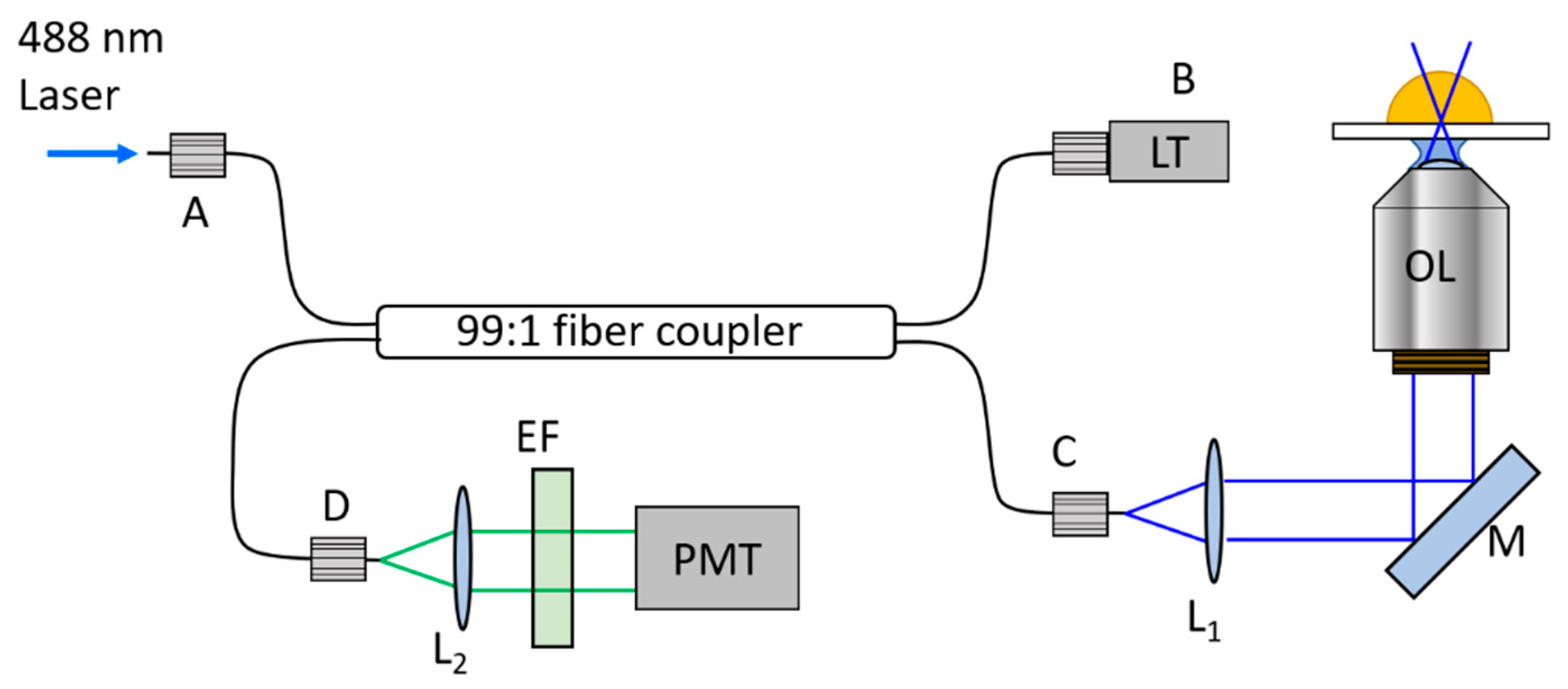
2.1. Fiber-Optic Based Fluorescence Correlation Spectroscopy (FB-FCS)

Figure 1 shows the experimental setup of the FB-FCS system. The excitation light source was a laser diode (LP488-SF20, Thorlabs, Newton, USA) with a wavelength of 488 nm. The excitation laser, whose spectrum was narrowed by a laser line filter (FL488-1, Thorlabs, Newton, USA), was coupled to port A of a 99:1 fiber coupler (FC488-99B-FC, Thorlabs, Newton, USA). 99% of the laser was output from port B and absorbed by a light trap (LT) (FTFC1, Thorlabs, Newton, USA). The remaining 1% of the laser was output from port C and collimated by a lens (L₁) with a focal length of 40 mm. The laser was focused on fluorescent samples on coverslips using a water immersion objective lens (OL) (UPlanSApo 60×/1.20 W, Olympus, Tokyo, Japan). The diameter of the excitation laser spot (the diameter of the Airy disk) is 496 nm in an ideal setup. The emitted fluorescence of the Airy disk pattern with a diameter of 6.62 µm was imaged on the end surface of port C. The mode field diameter of the optical fiber was 3.5 µm at 515 nm. The end surface of port C played the role of a pinhole, and its diameter was estimated to be approximately 0.53 Airy units. The position of the focal spot of the objective lens and fiber core of the fiber coupler at port C were always optically conjugated. Thus, precise pinhole adjustment is not necessary for FB-FCS. Adjustment of the correction ring of the objective lens depending on the thickness of the coverslip makes the sensitivity of the system higher. The fluorescence imaged on port C was coupled to the fiber coupler, and 99% was output from port D. Finally, the fluorescence was detected by a single photon counting module using a photomultiplier tube (PMT) (H7421-40, HPK, Hamamatsu, Japan) via a lens L₂ and emission filter (EF) (FF01-525/39-25, IDEX Health & Science, New York, USA).

The TTL signal from the PMT was transformed into an autocorrelation function (ACF) using a hardware correlator (10CX220YU484I6G, APOLLO, Yokohama, Japan). The time resolution of the correlator is variable in the range of 10-1,280 ns because it is constructed using a field-programmable gate array (FPGA) chip. The time resolution of the ACF was set to 640 ns in this study.

2.2. Background Intensity Correction

In FCS, background intensity lowers the amplitude of the ACF, resulting in an overestimation of concentration. The background intensity of conventional FCS can be considered negligible in most cases because it is sufficiently lower than the fluorescence signal intensity. However, the background intensity of FB-FCS is higher than that of conventional FCS because of contamination from the excitation laser, which is reflected at the end surface and inside the fiber coupler. The photon count of this background intensity is approximately 150 kHz with a 1 μW excitation laser power at the sample plane in our setup. The main source of such a high background was likely due to the autofluorescence of the optical fibers as reported by Garai et al. [11]. In addition, strong reflection and scattering of excitation laser at the end surface of each fiber and back reflection at the junction of the optical fibers inside the fiber coupler might be also the source.

To correct this background intensity effect on the obtained ACF, we applied the following background intensity correction [5,12]:

$$G_{\mathrm{c}}\left(\tau \right)={\left(\frac{\overline{I}}{\overline{I}-{\overline{I}}_{\mathrm{bg}}}\right)}^{2}G\left(\tau \right),$$

(1)

where $G$ and $G_{\mathrm{c}}$ are the measured ACF and the ACF with background intensity correction, respectively. $\overline{I}$ and ${\overline{I}}_{\mathrm{bg}}$ are the average fluorescence intensity and the average background intensity, respectively. The average background intensity is usually measured on blank samples, such as pure water and pure solvent of the sample solution. Note that the factor ${\left[\overline{I}/\left(\overline{I}-{\overline{I}}_{\mathrm{bg}}\right)\right]}^2$ becomes very high. Thus, $\overline{I}$ and ${\overline{I}}_{\mathrm{bg}}$ should be carefully determined especially in low concentration samples.

2.3. Fitting Analysis

Non-linear least-squares analysis was performed on the background-corrected ACFs using QuickFit 3.0 [13]. A 3D free diffusion model with one diffusion component and one non-fluorescent component was adopted for the fitting analysis. The model equation is defined as follows [12,14]:

$$G\left(\tau \right)=\frac{1-\theta +\theta \exp \left(-\frac{\tau }{{\tau }_{\mathrm{T}}}\right)}{N\left(1-\theta \right)}{\left(1+\frac{\tau }{{\tau }_{\mathrm{D}}}\right)}^{-1}{\left(1+\frac{1}{{\gamma }^2}\frac{\tau }{{\tau }_{\mathrm{D}}}\right)}^{-1/2}+G_{\infty },$$

(2)

where $N$ and ${\tau }_{\mathrm{D}}$ are the number of molecules inside the measurement volume (confocal volume) and the diffusion time, which is proportional to the hydrodynamic diameter of the fluorescent molecule. $\gamma$ is the structure parameter, which is the aspect ratio between the axial and lateral radii of the measurement volume. The structure parameter is expected to be 3–6 for a one-photon excitation system [15]. The structure parameter was fixed at 5.0 in the fitting analysis in this work. $\theta$ denotes the fraction of non-fluorescent components, including the triplet component and ${\tau }_{\mathrm{T}}$ denotes its decay time. $G_{\infty }$ is the offset of the autocorrelation function.

3. Results and Discussion

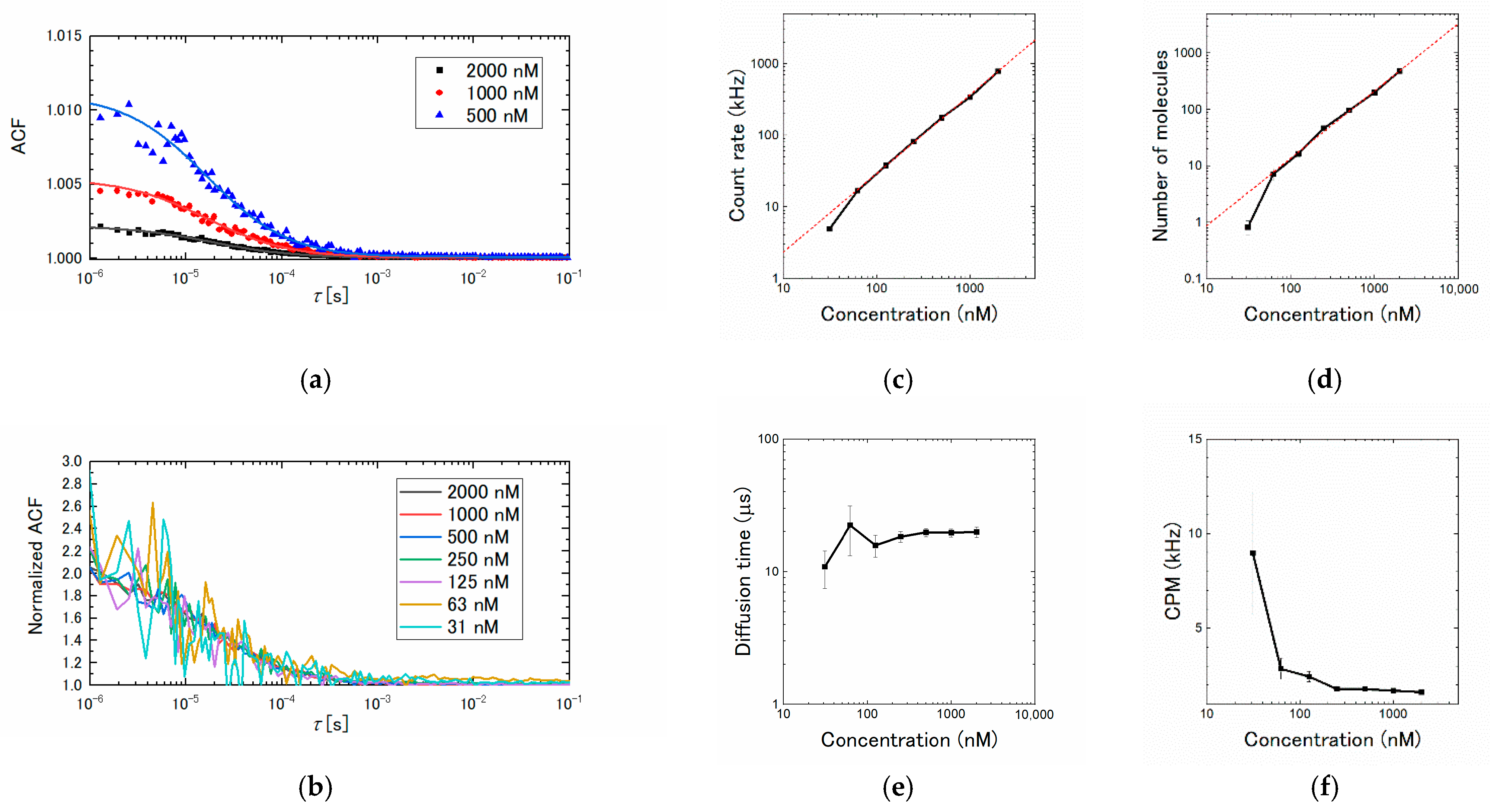
3.1. Concentration Dependence

The concentration dependence of FB-FCS was first confirmed using an organic fluorescent dye, the NIST-traceable fluorescein standard. The fluorescein dilution series was prepared using a dilution buffer (100 mM borate buffer, pH 9.5). The results are shown in Figure 2. The measurement duration was 60 s. The excitation laser power was 1.1 μW at the focal plane of the objective lens. The background count rate was found to be 163.7 kHz using a dilution buffer as the sample.

Figure 2a shows the average ACFs measured for each concentration. The ACFs at low concentrations are not shown here to avoid the plot becoming too busy. The excluded plots are shown in Figure A1 in Appendix A. Because the amplitude of the ACF in FCS is inversely proportional to the number of molecules, the amplitudes of the results increased as the concentration decreased. Figure 2b shows the normalized ACFs. The amplitudes of the fluorescent components were normalized to unity based on the number of molecules obtained by the fitting analysis. The decay of each normalized ACF did not change significantly. This was because the diffusion speed was not changed by the concentration because the effect of the concentration of fluorescein on the viscosity can be considered negligible at low concentrations.

Figure 2c shows the linear relationship between the fluorescence count rate and the concentration. The red broken line is a regression line for concentrations ranging from 63 nM to 2000 nM ($y=1.10x-0.72$, $R^2=0.9992$). At low concentrations, the count rate was too low compared to the value predicted by the linear fitting line. This was likely due to the background correction error because of the long-term (time scale of several ten minutes) fluctuations in the laser power.

Figure 2d shows the linear relationship between the number of molecules and concentration. The red broken line is a regression line for concentrations ranging from 63 nM to 2000 nM ($y=1.19x-1.26$, $R^2=0.9977$). Good linearity was maintained above 63 nM, at least under these measurement conditions. The non-zero intercept of the regression line likely indicates that the system underestimated the number of fluorescein by 1.26. To measure sparser samples, a more stable excitation light source and elongation of the measurement duration are needed [16].

Figure 2e,f shows the results of the diffusion time and counts per molecule (CPM). The CPM is the brightness per single fluorescent molecule, defined by

$$\epsilon =\frac{\overline{I}-{\overline{I}}_{\mathrm{bg}}}{N}.$$

(3)

Both the diffusion time and CPM must be independent of the concentration. The concentration of samples needed to be more than 63 nM for diffusion time measurement and 250 nM for CPM measurement under these measurement conditions.

The lateral radius of measurement volume w₀ can be estimated as follows:

$$w_0=\sqrt{4D{\tau }_{\mathrm{D}}},$$

(4)

where D is a diffusion coefficient of the sample molecule. Using the known diffusion coefficient of $D$ = 436 μm²/s [17] and the measured diffusion time of 19.6 μs for 1000 nM fluorescein, we obtained w₀ = 185.0 nm. We can obtain the diffusion coefficient of an unknown sample using $w_0$ and Equation (4). Furthermore, we can determine the measurement volume of FB-FCS because we measured the fluorescein with a highly reliable concentration. The number of molecules can be expressed as follows [18]:

$$N=VC{N}_A,$$

(5)

where $V$, $C$, and $N_A$ are the measurement volume, concentration in molar concentration units, and Avogadro’s number. Using the slope of 1.19, from the results of Figure 2d and Equation (5), we obtained a measurement volume of 1.98 fL.

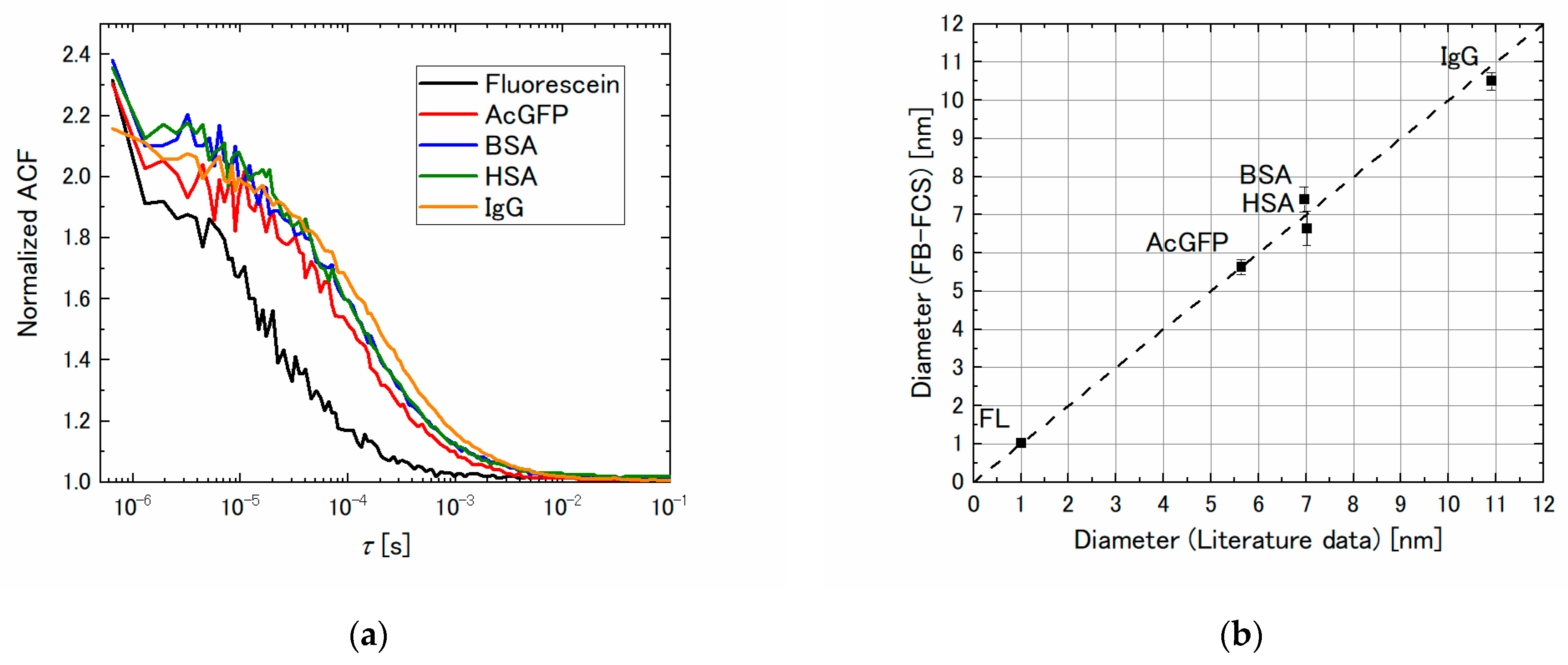
3.2. Molecular Size Dependence

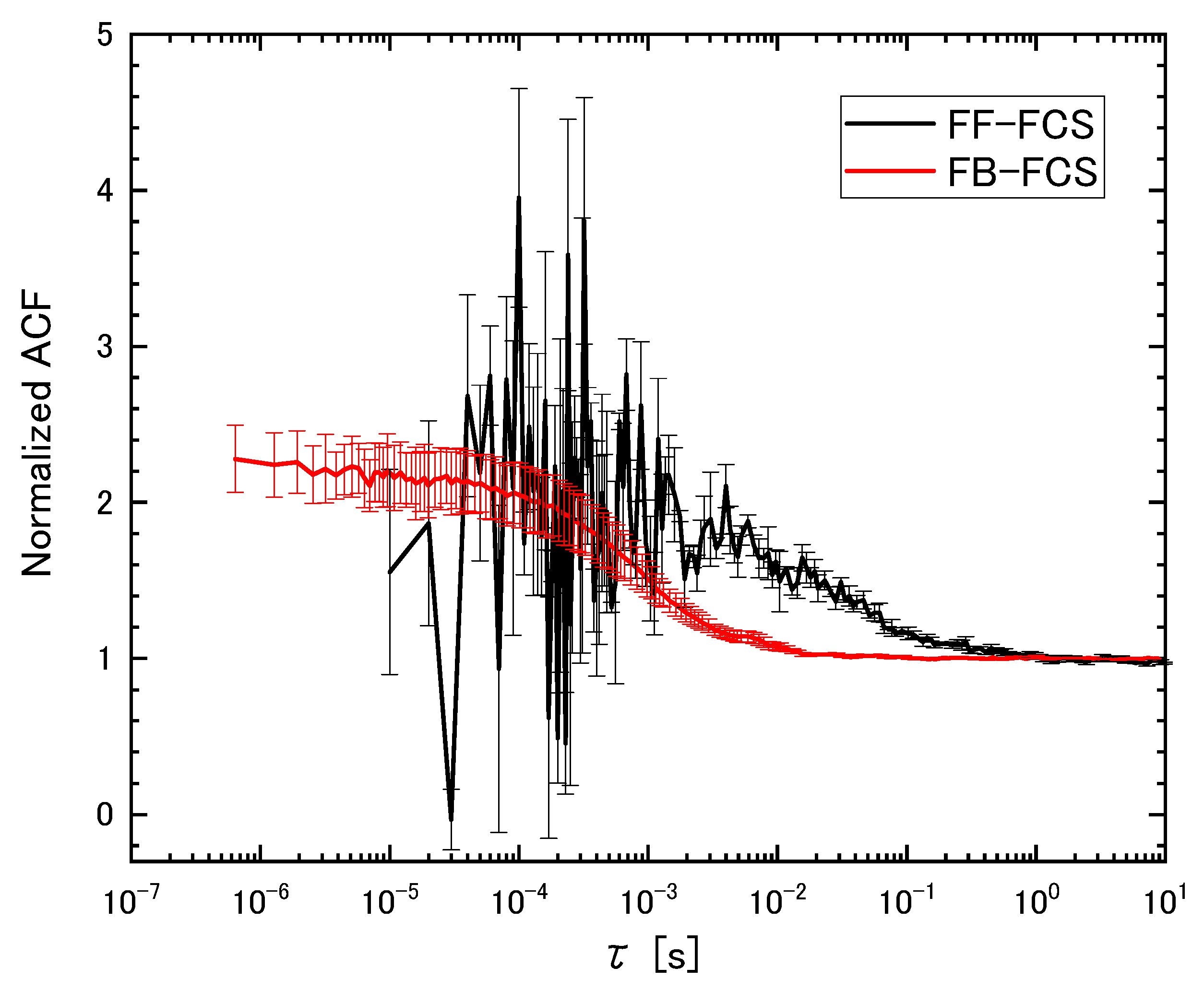
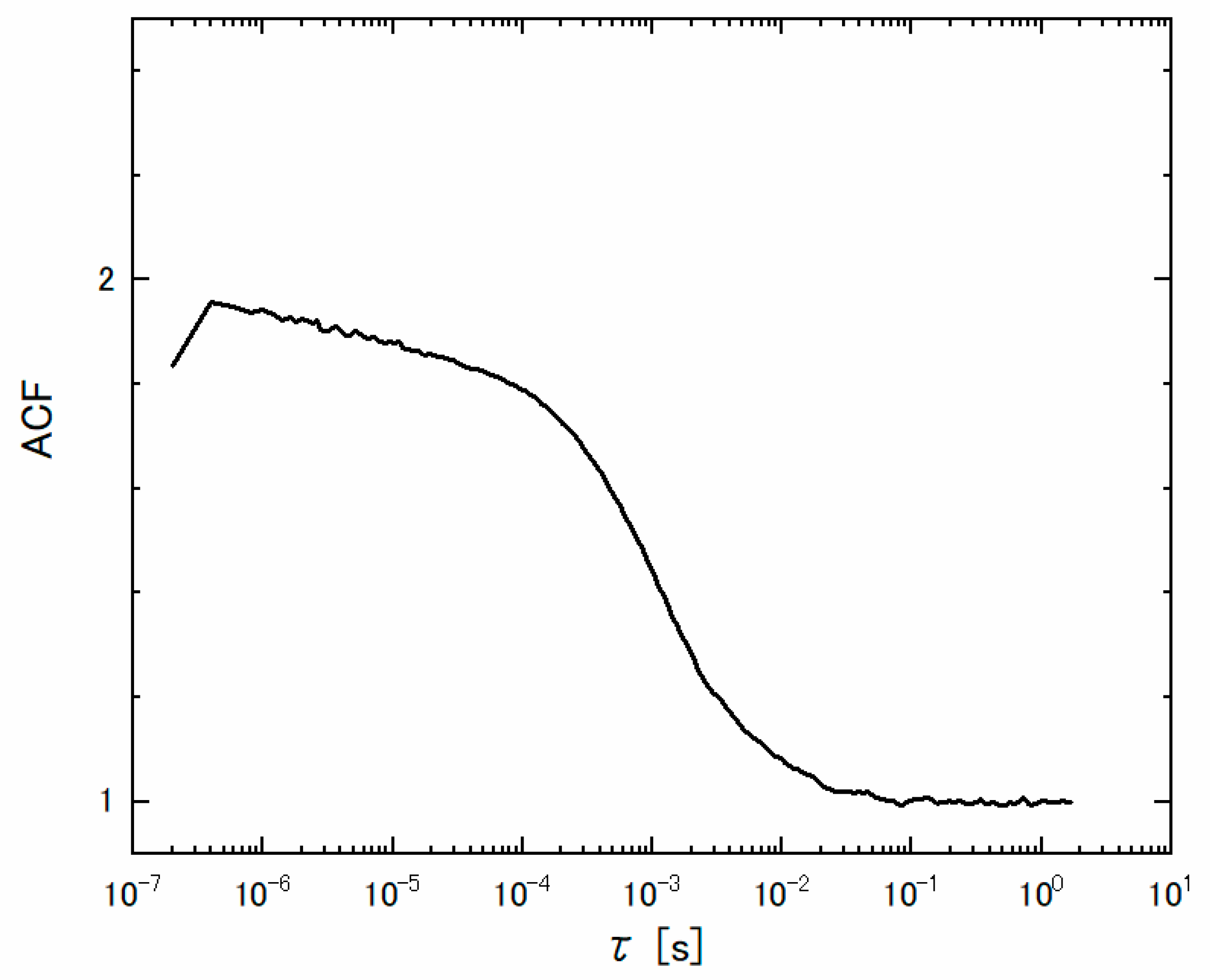
Figure 3 shows the molecular size dependence of the ACF. The samples were fluorescein, recombinant Aequorea coerulescens GFP (AcGFP), and ATTO 488 labeled proteins, bovine serum albumin (BSA), human serum albumin (HSA), and immunoglobulin G (IgG). Furthermore, we estimated the hydrodynamic diameter of the sample molecules using the Einstein–Stokes relationship:

$$D=\frac{k_{\mathrm{B}}T}{3\pi \eta d},$$

(6)

where $k_{\mathrm{B}}$, $T$, $\eta$, and $d$ are the Boltzmann constant, absolute temperature, the viscosity of the solvent, and diameter of the molecule, respectively. The estimated diameters and data from the literature are compared in

Table 1. Measurement Results of Various Samples. The diameter of FB-FCS shows mean ± standard error (n = 5–8).

Sample	FB-FCS	Literature Value
	Diametera [nm]	Diameter [nm]	Ref.
Fluorescein	1.01 ± 0.07	1.00	[19]
AcGFP	5.63 ± 0.19	5.64	[20]
BSA	7.39 ± 0.33	6.96	[21]
HSA	6.65 ± 0.44	7.0	[22]
IgG	10.50 ± 0.23	10.9	[23]

. Figure 3a shows the normalized ACF of each sample. The larger the molecules, the longer the decay time of the ACFs. Figure 3b compares the diameters measured by FB-FCS and those reported in the literature. The values are also listed in Table 1. The diameters obtained by FB-FCS were in good agreement with those reported in the literature, indicating that FB-FCS could measure molecular size precisely even without any mechanical adjustment of the optical setup.

3.3. Robustness

To validate the robustness of the FB-FCS system, the same sample was measured on different days for two weeks without any mechanical adjustment, as shown in Figure 4. The sample consisted of green fluorescent beads with a diameter of 0.04 μm (Polystyrene Fluorescent Microspheres, Dragon Green, FSDG001, Cosmo Bio, Tokyo, Japan). The beads were diluted to a concentration of 0.41 μM using pure water. The 10-s measurement was repeated 15 times, and the averaged ACF was analyzed each day. There was almost no difference in the shape of the normalized ACFs for two weeks, as shown in Figure 4a. In addition, neither the diffusion time nor the CPM showed a large difference, as shown in Figure 4b,c. The mean diffusion time in a day was 1154.1 ± 54.3 ms (mean ± standard deviation), and its coefficient of variation was 4.7%. The mean CPM in the days was 572.4 ± 24.5 kHz (mean ± standard deviation), and its coefficient of variation was 4.3%. These results indicate that reliable and reproducible FCS data can be obtained without any adjustment of the developed system.

4. Conclusions

In this study, we developed a new FCS system called FB-FCS by introducing a water immersion objective lens to focus the excitation laser. Measurements of the concentration and molecular size were successfully performed.

The fluorescence sensitivity was still lower than conventional FCS instruments because of fluorescence loss by fiber optics. However, that was sufficient to measure the solutions of the fluorescent dye monomer. This is a very important improvement for biological and biomedical applications. The fluorescence sensitivity (CPM per excitation laser power, CPM/LP) of FB-FCS was improved 1168 times higher than it of the FF-FCS system (Figure A2 and

Table A1. Measurement results of fluorescent latex beads. The values show mean ± standard error (n = 3). Conv. FCS denotes the conventional FCS system.

	τD [ms]	CPM [kHz]	CPM/LP [kHz/μW]
FF-FCS	18.26 ± 1.95	0.17 ± 0.01	0.023 ± 0.002
FB-FCS	0.57 ± 0.02	80.16 ± 2.42	27.35 ± 0.82
Conv. FCS	1.07 (n = 1)	65.57 (n = 1)	43.71 (n = 1)

in Appendix B). Furthermore, the sensitivity of FB-FCS reached 62.6% of a conventional FCS system (307-15471, Wako, Osaka, Japan) as shown in Figure A3 and Table A1.

The concentration measurement showed good linearity in the region above 63 nM. To measure a lower-concentration sample, the measurement duration should be extended. The molecular diameters measured by FB-FCS and the corresponding values reported in the literature also showed good linearity.

Finally, the robustness of FB-FCS was validated. Both the diffusion time and CPM were stable for two weeks, and the coefficients of variation were less than 5% without any mechanical adjustment.

These results indicate that FB-FCS can be used instead of the conventional FCS system to measure the concentration and size of target molecules. However, this system cannot take microscopic images, unlike a conventional FCS system based on the frame of a microscope. Therefore, it is difficult to determine the measurement position in the cell for FB-FCS. The conventional FCS system might be suitable for such in vivo FCS measurements.

The FB-FCS system does not require any mechanical adjustment of the optical setup. Furthermore, FB-FCS is low-cost and compact compared to conventional FCS instruments. For these reasons, the availability of FB-FCS may be higher than that of high-spec FCS systems. We expect that the FB-FCS system will be used as a simple measurement system in laboratories, medical diagnosis, and environmental measurements.

References

1. Elson, E.L.; Magde, D. Fluorescence correlation spectroscopy. I. Conceptual basis and theory. Biopolymers 1974, 13, 1–27. [Google Scholar] [CrossRef]
2. Aragón, S.R.; Pecora, R. Fluorescence correlation spectroscopy as a probe of molecular dynamics. J. Chem. Phys. 1976, 64, 1791–1803. [Google Scholar] [CrossRef]
3. Rigler, R.; Mets, Ü.; Widengren, J.; Kask, P. Fluorescence correlation spectroscopy with high count rate and low background: Analysis of translational diffusion. Eur. Biophys. J. 1993, 22, 169–175. [Google Scholar] [CrossRef]
4. Rauer, B.; Neumann, E.; Widengren, J.; Rigler, R. Fluorescence correlation spectrometry of the interaction kinetics of tetramethylrhodamin α-bungarotoxin with Torpedo californica acetylcholine receptor. Biophys. Chem. 1996, 58. [Google Scholar] [CrossRef]
5. Oasa, S.; Sasaki, A.; Yamamoto, J.; Mikuni, S.; Kinjo, M. Homodimerization of glucocorticoid receptor from single cells investigated using fluorescence correlation spectroscopy and microwells. FEBS Lett. 2015, 589, 2171–2178. [Google Scholar] [CrossRef] [PubMed] [Green Version]
6. Shen, C.; Knapp, M.; Puchinger, M.G.; Shahzad, A.; Gaubitzer, E.; Shen, A.D.; Koehler, G. Using fluorescence correlation spectroscopy (FCS) for IFN-g detection: A preliminary study. J. Immunol. Methods 2014, 407, 35–39. [Google Scholar] [CrossRef]
7. Chatterjee, M.; Nöding, B.; Willemse, E.A.J.; Koel-Simmelink, M.J.A.; van der Flier, W.M.; Schild, D.; Teunissen, C.E. Detection of contactin-2 in cerebrospinal fluid (CSF) of patients with Alzheimer’s disease using Fluorescence Correlation Spectroscopy (FCS). Clin. Biochem. 2017, 50, 1061–1066. [Google Scholar] [CrossRef]
8. Fujii, F.; Horiuchi, M.; Ueno, M.; Sakata, H.; Nagao, I.; Tamura, M.; Kinjo, M. Detection of prion protein immune complex for bovine spongiform encephalopathy diagnosis using fluorescence correlation spectroscopy and fluorescence cross-correlation spectroscopy. Anal. Biochem. 2007, 370, 131–141. [Google Scholar] [CrossRef]
9. Sahoo, B.; Sil, T.B.; Karmakar, B.; Garai, K. A Fluorescence Correlation Spectrometer for Measurements in Cuvettes. Biophys. J. 2018, 115, 455–466. [Google Scholar] [CrossRef] [Green Version]
10. Singh, N.K.; Chacko, J.V.; Sreenivasan, V.K.A.; Nag, S.; Maiti, S. Ultracompact alignment-free single molecule fluorescence device with a foldable light path. J. Biomed. Opt. 2011, 16, 025004. [Google Scholar] [CrossRef]
11. Garai, K.; Muralidhar, M.; Maiti, S. Fiber-optic fluorescence correlation spectrometer. Appl. Opt. 2006, 45, 7538–7542. [Google Scholar] [CrossRef]
12. Yamamoto, J.; Kinjo, M. Full fiber-optic fluorescence correlation spectroscopy. Opt. Express 2019, 27, 14835. [Google Scholar] [CrossRef]
13. Krieger, J.W.; Singh, A.P.; Bag, N.; Garbe, C.S.; Saunders, T.E.; Langowski, J.; Wohland, T. Imaging fluorescence (cross-) correlation spectroscopy in live cells and organisms. Nat. Protoc. 2015, 10, 1948–1974. [Google Scholar] [CrossRef]
14. Widengren, J.; Mets, U.; Rigler, R. Fluorescence correlation spectroscopy of triplet states in solution: A theoretical and experimental study. J. Phys. Chem. 1995, 99, 13368–13379. [Google Scholar] [CrossRef]
15. Kim, S.A.; Heinze, K.G.; Schwille, P. Fluorescence correlation spectroscopy in living cells. Nat. Methods 2007, 4, 963–973. [Google Scholar] [CrossRef] [PubMed]
16. Saffarian, S.; Elson, E.L. Statistical Analysis of Fluorescence Correlation Spectroscopy: The Standard Deviation and Bias. Biophys. J. 2003, 84, 2030–2042. [Google Scholar] [CrossRef] [Green Version]
17. Petrášek, Z.; Schwille, P. Precise Measurement of Diffusion Coefficients using Scanning Fluorescence Correlation Spectroscopy. Biophys. J. 2008, 94, 1437–1448. [Google Scholar] [CrossRef] [PubMed] [Green Version]
18. Sasaki, A.; Yamamoto, J.; Kinjo, M.; Noda, N. Absolute Quantification of RNA Molecules Using Fluorescence Correlation Spectroscopy with Certified Reference Materials. Anal. Chem. 2018, 90, 10865–10871. [Google Scholar] [CrossRef] [PubMed] [Green Version]
19. Mustafa, M.B.; Tipton, D.L.; Barkley, M.D.; Russo, P.S.; Blum, F.D. Dye diffusion in isotropic and liquid-crystalline aqueous (hydroxypropyl)cellulose. Macromolecules 1993, 26, 370–378. [Google Scholar] [CrossRef]
20. Terry, B.R.; Robards, A.W. Hydrodynamic radius alone governs the mobility of molecules through plasmodesmata. Planta 1987, 171, 145–157. [Google Scholar] [CrossRef]
21. Ikeda, S.; Nishinari, K. Intermolecular Forces in Bovine Serum Albumin Solutions Exhibiting Solidlike Mechanical Behaviors. Biomacromolecules 2000, 1, 757–763. [Google Scholar] [CrossRef] [PubMed]
22. Naeem, A.; Amani, S. Deciphering Structural Intermediates and Genotoxic Fibrillar Aggregates of Albumins: A Molecular Mechanism Underlying for Degenerative Diseases. PLoS ONE 2013, 8, e54061. [Google Scholar] [CrossRef] [Green Version]
23. Bermudez, O.; Forciniti, D. Aggregation and denaturation of antibodies: A capillary electrophoresis, dynamic light scattering, and aqueous two-phase partitioning study. J. Chromatogr. B 2004, 807, 17–24. [Google Scholar] [CrossRef] [PubMed]
Figure 1. Experimental setup. LT, light trap. L, lens. M, mirror. OL, objective lens. EF, emission filter. PMT, photomultiplier tube.
Applsci 11 06744 g001
Figure 2. FB-FCS measurements on fluorescein solution. (a) Average ACF at different concentrations (n = 5). The symbols show the measurement results. Solid lines are the fitting curves. (b) Average normalized ACFs (n = 5). (c) Linear relationship between fluorescence count rate and concentration. The background count rate was subtracted. (d) Linear relationship between the measured number of molecules and concentration. (e) Measured diffusion time at each concentration. (f) Measured CPM at each concentration. (c,f) Error bars show standard error (n = 5). Red broken lines show the results of the linear fitting.
Applsci 11 06744 g002
Figure 3. FB-FCS measurements on fluorescently labeled proteins. (a) Normalized ACFs. (b) Comparison between diameters measured by FB-FCS and results from the literature. The dashed line shows the y = x line. The error bar represents the standard error (n = 5–8). FL denotes the data point of fluorescein.
Applsci 11 06744 g003
Figure 4. FB-FCS measurements on fluorescent beads on different days. (a) Normalized ACFs. (b) Diffusion time. (c) CPM.
Applsci 11 06744 g004