Reactive Balance Control for Legged Robots under Visco-Elastic Contacts

Abstract

Contacts between robots and environment are often assumed to be rigid for control purposes. This assumption can lead to poor performance when contacts are soft and/or underdamped. However, the problem of balancing on soft contacts has not received much attention in the literature. This paper presents two novel approaches to control a legged robot balancing on visco-elastic contacts, and compares them to other two state-of-the-art methods. Our simulation results show that performance heavily depends on the contact stiffness and the noises/uncertainties introduced in the simulation. Briefly, the two novel controllers performed best for soft/medium contacts, whereas “inverse-dynamics control under rigid-contact assumptions” was the best one for stiff contacts. Admittance control was instead the most robust, but suffered in terms of performance. These results shed light on this challenging problem, while pointing out interesting directions for future investigation.

1. Introduction

1.1. Problem Overview

Balance control of legged robots is a fundamental problem in robotics and is at the heart of numerous recent publications in the literature [1]. In this task, depending on whether the contact between the robot and the environment is rigid or soft, the robot will behave differently. However, for the sake of simplicity, a large part of studies has focused on the problem of controlling the balance of a rigid robot in contact with a rigid environment [2,3,4,5,6,7]. In this scenario, theoretically, the contact forces between the robot and the environment can be modified instantaneously. This is no longer possible if the environment is visco-elastic, or, equivalently, if a visco-elastic element is located between the robot actuators and the contact points, as in many legged robots which include soft elements at the ankles or the feet [7,8,9,10]. These compliant elements are extremely useful: they absorb impact during walking/running, protect the mechanical structure, tend to improve the quality of force measurements, and can make walking more efficient [10]. Moreover, the assumption of rigid contact is always an approximation because in the real world all contacts are visco-elastic up to a certain extent. In the presence of elasticity, the contact forces cannot be instantaneously modified, but their derivative—either of first or second order—can be modified depending on the contact damping (as detailed in Section 2). Despite the popularity of visco-elastic elements, balancing on visco-elastic contacts is still an open problem. This question is at the heart of the paper. It is addressed through the introduction of two new compliant controllers and a comparative study with existing strategies.

1.2. State of the Art

The most common approach is to neglect elasticity in the balance controller and simply assume that contacts are rigid. This method works fine for contacts that are not too soft and that are sufficiently well damped, as was demonstrated with a passivity-based controller on the Toro humanoid robot [11]. However, in general, making this hypothesis results in destabilizing oscillations [1]. Force feedback can then be used for damping these oscillations. This is usually done by using force feedback to modify the position references given to a high-gain joint position controller, leading to admittance-control schemes [5,7,9]. Although this approach proved to be successful in practice, its lack of theoretical foundations makes it challenging to tune and analyze in a robust and repeatable way.

A crucial issue of admittance-control schemes is the resulting delay in the force tracking. To deal with it, two approaches have been proposed so far. The first one [3] is to prove that the controller is robust to these delays. The second one is to account for the delay by introducing a 1-st order low-pass filter in the dynamic model used by balance controller. Our analysis reveals that the force tracking delay is actually not an issue, so long as the admittance-control gains are properly set.

Instead of relying on admittance control, another approach is to try to change the contact forces at the next time step [12] since they cannot be changed instantaneously. This approach exploits a model of the visco-elastic contacts for the controller design. However, as it mainly relies on contact damping, it cannot be applied if the damping is too low (see Section 2.1).

Recently, the state-of-the-art Whole-Body Controller [13] has been extended to ensure consistency to terrain compliance [14]. In this approach the controller incorporated a soft-contact model and was connected with an online learning algorithm that estimates the terrain compliance. Though that work focused on the case of well-damped contacts, we focus here on the underdamped case.

1.3. Contributions

The contribution of this paper is two-fold. First two novel strategies are introduced for controlling the balance of legged robots under visco-elastic contacts with their environment. The proposed approach unifies position and force feedback, leading to a simple gain-tuning procedure for which standard tools from linear system control can be used (e.g., LQR, pole placement). Second, a thorough comparison of different controllers is proposed for different kinds of compliant contact and noisy measurements to discuss the efficiency of the different approaches. More precisely, the two novel controllers that were designed to deal with visco-elastic contacts are compared in simulation with two state-of-the-art approaches for the same stabilization task of a model of the lateral dynamics of HRP-2 in double support and under different contact stiffnesses and noisy conditions. The study highlights pros and cons of each method according to the different parameters and demonstrates the performance of the proposed controllers in case of compliant contact.

Even though the paper mainly focuses on legged robots, the results are also of great interest for manipulation problems for which the control of compliant contacts is required.

1.4. Paper Structure

Section 2 introduces the visco-elastic contact model and the robot dynamics. Section 3 summarizes two state-of-the-art methods. The first one (Section 3.1) is classically used for rigid contacts (TSID-Rigid [4]). The second one (Section 3.2) is an admittance-control scheme (Adm-Ctrl) relying on joint position control [8]. Section 4 presents an extension of Adm-Ctrl (TSID-Adm), while Section 5 proposes a novel approach to balance on elastic contacts (TSID-Flex-K). Section 6 presents simulation results comparing the four methods. Finally, Section 7 concludes the paper.

2. Background: Dynamics and Contact Model

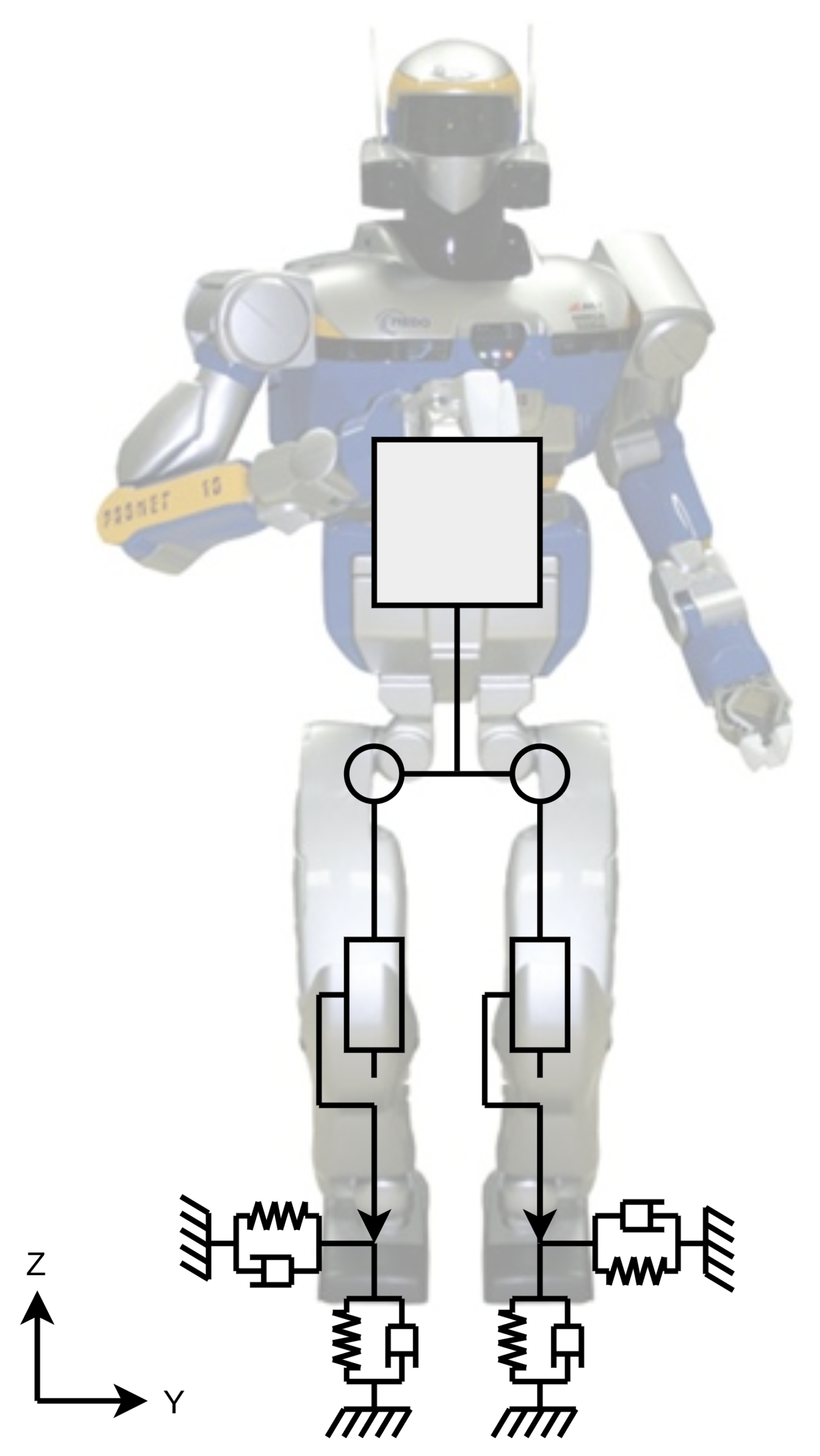
2.1. Visco-Elastic Contact Model

Consider a robot in contact with the environment at k contact points. We assume that the contact surfaces are visco-elastic, or, equivalently, the robot is equipped with visco-elastic elements between each contact point and the last actuator of the corresponding kinematic chain. In the latter case, we can model the part of the robot after the visco-elastic element as part of the environment, and the contact point as the last point of the robot before the visco-elastic element. We also assume that each contact force $f_i\in {\mathbb{R}}^3$ is proportional to the induced contact position $p_i\in {\mathbb{R}}^3$ and velocity ${\dot{p}}_i\in {\mathbb{R}}^3$:

$$f_i=K_i(p_i^0-p_i)-B_i{\dot{p}}_i,\forall i\in [1..k]$$

(1)

where $K_i,B_i\in {\mathbb{R}}^{3\times 3}$ are the positive-definite diagonal stiffness and damping matrices, respectively, and $p_i^0\in {\mathbb{R}}^3$ is the contact position corresponding to a null force. Stacking all contact forces together we can rewrite (1) as:

$$f=K(p_0-p)-B\dot{p}$$

(2)

Given that contacts are unilateral, this model is valid as long as normal forces are positive (i.e., pushing). Since the contact forces are function of the robot configuration, we cannot change them instantaneously as in the rigid contact case, because of the finite maximum acceleration of the actuation. However, if $B\ne 0$, we can affect their time derivative through the contact point accelerations $\ddot{p}$:

$$\dot{f}=-K\dot{p}-B\ddot{p}$$

(3)

If instead $B\approx 0$, we can only affect the second time derivative of f:

$$\ddot{f}=-K\ddot{p}$$

(4)

2.2. Importance of Stiffness vs. Damping

Our main interest lies in the underdamped case—which is more challenging in our experience—which means that $B\ll 2\sqrt{K}$ ($B=2\sqrt{K}$ correspond to the critically damped case). In these cases, relying on (3) to control $\dot{f}$ may not be convenient because very large values of $\ddot{p}$ (hence motor commands) may be required.

Appendix C includes an order-of-magnitude analysis that supports this claim for the usual dynamics of humanoid robots and illustrates why we prefer to rely on (4) rather than on (3) for our controller design.

2.3. Centroidal Dynamics

To balance a legged robot, we must control its CoM c and its angular momentum l. The dynamics of these two quantities is described by the Newton–Euler equations, where all quantities are expressed in an arbitrary inertial frame with z aligned with gravity:

$$m\ddot{c}=\sum _{i=1}^k{f}_i+mg$$

(5)

$$\dot{l}=\sum _{i=1}^k(p_i-c)\times f_i$$

(6)

where $m\in {\mathbb{R}}^{}$ is the robot mass, and $g=(0,0,-9.81)$ is the gravity acceleration. We can write (5) and (6) in matrix form as:

$$\begin{array}{c}\hfill \underset{\ddot{x}}{\underbrace{\left[\begin{array}{c}m\ddot{c}\\ \dot{l}\end{array}\right]}}=\underset{A}{\underbrace{\left[\begin{array}{ccc}{I}_3& \cdots & I_3\\ {(p_1-c)}_{\times }& \cdots & {(p_k-c)}_{\times }\end{array}\right]}}\underset{f}{\underbrace{\left[\begin{array}{c}{f}_1\\ ⋮\\ f_k\end{array}\right]}}+\underset{b}{\underbrace{\left[\begin{array}{c}mg\\ 0_3\end{array}\right]}},\end{array}$$

(7)

where $y_{\times }\in {\mathbb{R}}^{3\times 3}$ is the cross-product matrix associated with y.

2.4. Whole-Body Dynamics

The dynamics of a floating-base robot with n joints is described by the following equations:

$$M\dot{v}+h-J^{\top }f=S^{\top }\tau ,$$

(8)

where $M\in {\mathbb{R}}^{(n+6)\times (n+6)}$ is the mass matrix, $v\in {\mathbb{R}}^{n+6}$ is the robot velocity vector, $h\in {\mathbb{R}}^{n+6}$ contains the gravitational, centrifugal and Coriolis forces, $J\in {\mathbb{R}}^{3k\times (n+6)}$ is the contact Jacobian, $S=\left[\begin{array}{cc}{0}_{n\times 6}& I_{n\times n}\end{array}\right]\in {\mathbb{R}}^{n\times (n+6)}$ is the selection matrix of the actuated joints, and $\tau \in {\mathbb{R}}^n$ are the joint torques. The same dynamics can be expressed by splitting the first 6 rows, which correspond to the unactuated floating base, from the last n rows, which correspond to the actuated joints:

$$M_u\dot{v}+h_u-J_u^{\top }f=0$$

(9)

$$M_a\dot{v}+h_a-J_a^{\top }f=\tau$$

(10)

Equation (9) is equivalent to the centroidal dynamics [15] and is sufficient to ensure dynamic consistency in the controllers based on Task-Space Inverse Dynamics (TSID) [4]. Finally, the relationship between the accelerations of the contact points and the robot configuration is given by:

$$\ddot{p}=J\dot{v}+\dot{J}v$$

(11)

This expression is obtained by derivative of the kinematic related to the contact point p: $\dot{p}=Jv$.

3. State of the Art

3.1. Inverse Dynamics with Rigid Contacts (TSID-Rigid)

This section summarizes the classic approach for balancing a legged robot in rigid contact with the environment [4].

The desired momentum rate of change is typically computed with a simple PD control law:

$${\ddot{x}}_d=\left[\begin{array}{c}m{\ddot{c}}_d\\ {\dot{l}}_d\end{array}\right]=\left[\begin{array}{c}m{\ddot{c}}^{*}+K_d^{com}{\dot{e}}_c+K_p^{com}{e}_c\\ {\dot{l}}^{*}+K_d^{am}{\dot{e}}_l+K_p^{am}{e}_l\end{array}\right],$$

(12)

where $e_c$ and $e_l$ are the tracking error of the linear and angular part of the centroidal state, respectively. Often, the proportional part of the angular momentum feedback is neglected, but we use it here to ensure stability [6]. The contact forces and the robot accelerations are computed by solving the following least-squares problem:

$$\begin{array}{cc}\underset{\dot{v},f}{minimize}& \parallel Af-{\ddot{x}}_d{+b\parallel }^2+w_f\left|\right|f-f^{*}{\left|\right|}^2+w_{post}\left|\right|{\dot{v}}^{post}-\dot{v}{\left|\right|}^2\hfill \\ subject\; to& M_u\dot{v}+h_u=J_u^{\top }f\hfill \\ & J\dot{v}+\dot{J}v=0\hfill \\ & |M_a\dot{v}+h_a-J_a^{\top }f|\le {\tau }^{max}\hfill \\ & Bf\le 0,\hfill \end{array}$$

(13)

where $w_f\in {\mathbb{R}}^{}$ is the weight and $f^{*}\in {\mathbb{R}}^{3k}$ is the reference of the force regularization task, $w_{post}\in {\mathbb{R}}^{}$ is the weight of the postural task, the first constraint represents the centroidal dynamics, the second one is the rigid-contact constraint, the third constraint represents the joint torque limits, and the last one represents the friction cone limits. The reference postural task accelerations are:

$${\dot{v}}^{post}=K_p^{post}{e}_q(q^{*},q)-K_d^{post}v,$$

(14)

where $K_p^{post},K_d^{post}\in {\mathbb{R}}^{(n+6)\times (n+6)}$ are positive-definite diagonal gain matrices, $q^{*}\in SE\left(3\right)\times {\mathbb{R}}^n$ is a given reference posture, and $e_q(q_1,q_2)$ is an error function mapping two configurations $q_1,q_2\in SE\left(3\right)\times {\mathbb{R}}^n$ to the log of their relative displacement. Once the optimal contact forces $f_d$ and robot accelerations ${\dot{v}}_d$ are found, we compute the desired joint torques using (10). Please note that this approach does not require (nor exploit) any force measurement.

3.2. Admittance Control (Adm-Ctrl)

A classic way to control the contact wrenches in case of flexible contacts is to rely on admittance control. Several versions of admittance control exist and have been shown to perform well on real humanoid robots [7,8,16,17]. We decided to use the version with the minimum number of gains to simplify the gain-tuning procedure.

First, we compute the desired contact forces $f_d$ as:

$$\begin{array}{cc}\underset{f}{minimize}& \left|\right|Af-{\ddot{x}}_d+b{\left|\right|}^2\\ subject\; to& Bf\le 0,\end{array}$$

(15)

where ${\ddot{x}}_d$ is defined as in (12). We then compute the reference velocity of the contact points according to the force tracking error:

$${\dot{p}}_d=-K_f(f_d-f)$$

(16)

This reference velocity is directly used in an inverse kinematics (IK) algorithm to compute reference joint velocities. The IK is computed on each limb independently:

$${\dot{q}}_{jd}={\left(J{S}^{\top }\right)}^{†}{\dot{p}}_d$$

(17)

These joint velocities are then integrated and given to the high-gain position controller, which computes the joint torque commands:

$${\tau }_d=K_p^j(q_{jd}-q_j)-K_d^j{\dot{q}}_j$$

(18)

4. Inverse Dynamics Admittance Control (TSID-Adm)

To improve the performance of admittance control we suggest integrating it with an inverse dynamics control law. Once we have computed ${\dot{p}}_d$ with (16), we compute the desired contact point accelerations as:

$${\ddot{p}}^{*}=K_d^{adm}({\dot{p}}_d-\dot{p})$$

(19)

Finally, we rely on an inverse-dynamics control law to track these contact point accelerations:

$$\begin{array}{cc}\underset{\dot{v}}{minimize}& \parallel J\dot{v}+\dot{J}v-{\ddot{p}}^{*}{\parallel }^2+w_{post}\left|\right|{\dot{v}}^{post}-\dot{v}{\left|\right|}^2\\ subject\; to& M_u\dot{v}+h_u=J_u^{\top }\widehat{f}\\ & |M_a\dot{v}+h_a-J_a^{\top }\widehat{f}|\le {\tau }^{max}\end{array}$$

(20)

5. Flexible TSID (TSID-Flex-K)

This section presents an original control formulation, which consists of a standard feedback linearization. In the case of visco-elastic contacts we cannot directly control f, but only its first or second derivative. As already mentioned, since we are mainly interested in underdamped contacts, we assume we can only control $\ddot{f}$. Thus, we differentiate (7) twice and use (4) to express $x^{\left(4\right)}$ as a function of $\ddot{p}$:

$$\begin{array}{cc}{x}^{\left(4\right)}& =A\ddot{f}+2\dot{A}\dot{f}+\ddot{A}f\\ & =\underset{A_K}{\underbrace{(A_f-AK)}}\ddot{p}+\underset{a_K}{\underbrace{2\dot{A}\dot{f}-{\ddot{A}}_{c}f}},\end{array}$$

(21)

where:

$${\ddot{A}}_c\triangleq \left[\begin{array}{ccc}{0}_3& \cdots & 0_3\\ {\ddot{c}}_{\times }& \cdots & {\ddot{c}}_{\times }\end{array}\right]A_f\triangleq \left[\begin{array}{ccc}{0}_3& \cdots & 0_3\\ {f_1}_{\times }& \cdots & {f_k}_{\times }\end{array}\right]$$

(22)

5.1. Feedback Linearization

We can find the accelerations $\dot{v}$ that track at best the desired $x_d^{\left(4\right)}$ by solving the following least-squares problem [4]:

$$\begin{array}{cc}\underset{\dot{v}}{minimize}& \parallel A_{K}J\dot{v}+A_K\dot{J}v+a_K-x_d^{\left(4\right)}{\parallel }^2+\\ & w_{post}\left|\right|{\dot{v}}^{post}-\dot{v}{\left|\right|}^2\\ subject\; to& M_u\dot{v}+h_u=J_u^{\top }\widehat{f}\\ & |M_a\dot{v}+h_a-J_a^{\top }\widehat{f}|\le {\tau }^{max}\end{array}$$

(23)

where $\widehat{f}\in {\mathbb{R}}^{3k}$ are the measured/estimated contact forces. Once we have the optimal accelerations ${\dot{v}}_d$, we can compute the desired joint torques using (10) with $\dot{v}={\dot{v}}_d$ and $f=\widehat{f}$.

5.2. Accounting for Force Variations during the Time Step

Since we can only update the motor commands at discrete time steps, there is always an error due to state variations in between time steps. Normally, these errors are negligible because small state variations result in small variations of the quantities in (9) and (10). However, when the robot is in contact with a stiff environment, small displacements of the contact points lead to large variations of the contact forces. Therefore, we can improve performance by accounting for the variation of f during the time step, assuming the following approximated time evolution:

$$f\left(t\right)=f+t\dot{f}t\in [0,\delta t],$$

(24)

where $\delta t$ is the controller time step. Under this assumption the accelerations $\dot{v}$ vary during the time step. To get the desired average value of $\dot{v}$ during the time step the controller must compensate for the average value of f, which is:

$$f^{avg}=\widehat{f}+\frac{\delta t}{2}\widehat{\dot{f}}$$

(25)

In (23) we can thus replace $\widehat{f}$ with $\widehat{f}+\frac{\delta t}{2}\widehat{\dot{f}}$.

5.3. Linear Feedback Regulator

The least-squares problem (23) allows us to directly impose $x^{\left(4\right)}$—if it is compatible with the problem constraints. Thus, the resulting dynamics is a 4-th order integrator. We define x as the centroidal state $x=(mc,l^{\Sigma })$, where $l^{\Sigma }\in SO\left(3\right)$ should be the integral of the angular momentum. However, since this is not a measurable quantity [18], we approximate it with the orientation of the base link (which is typically the heaviest link), scaled by the 3D robot inertia. We then regulate x through a linear feedback control law:

$$\begin{array}{cc}{x}_d^{\left(4\right)}=& K_p^m{e}_x(x^{*},x)+K_d^m({\dot{x}}^{*}-\dot{x})+\\ & K_a^m({\ddot{x}}^{*}-\ddot{x})+K_j^m({\stackrel{⃛}{x}}^{*}-\stackrel{⃛}{x})+x^{\left(4\right)*},\end{array}$$

(26)

where $x^{*}\left(t\right)$ is a reference centroidal trajectory, and $e_x(x_1,x_2)$ is an error function mapping two centroidal states $x_1,x_2\in SE\left(3\right)$ to the log of their relative displacement. The diagonal positive-definite feedback gain matrices $K_p^m,K_d^m,K_a^m,K_j^m\in {\mathbb{R}}^{6\times 6}$ need to be chosen so that the closed-loop system be stable.

5.4. Friction Force Constraints

The inverse-dynamics least-squares problem typically contains a linear approximation of the force friction cone constraints. This is no longer possible in the case of visco-elastic contacts, because the contact forces are not a problem variable. However, we can still try to satisfy the friction cone constraints by bounding the contact force accelerations, which are affine functions of $\dot{v}$. This problem is similar to trying not to hit the joint position bounds by constraining the joint accelerations [19]. The friction cone constraints can be approximated by a set of linear constraints [4] of the form:

$$b^{\top }{f}_i\le 0$$

(27)

Using the approach of [19], given a bound on the force accelerations ${\ddot{f}}_{max}\in {\mathbb{R}}^3$ (i.e., $|{\ddot{f}}_i|\le {\ddot{f}}_{max}$), we can compute the maximum ${\dot{f}}_i$ in direction b such that it is possible to satisfy (27) in the future:

$$b^{\top }{\dot{f}}_i\le \sqrt{-2|b^{\top }{\ddot{f}}_{max}|\left(b^{\top }{f}_i\right)}$$

(28)

Even though ${\ddot{f}}_{max}$ depends on q, the method that we use [19] assumes constant acceleration bounds. Therefore, ${\ddot{f}}_{max}$ should be seen here as a user parameter that defines how conservative the algorithm should be. Putting together all the friction cone constraints as $Bf\le 0$ we can bound the force accelerations to ensure that (28) be satisfied at the next time step:

$$B\ddot{f}\le b_f^{max},$$

(29)

where $b_f^{max}$ is a function of f and $\dot{f}$ [19]. Finally, this constraint can be expressed as a function of $\dot{v}$:

$$-BK(J\dot{v}+\dot{J}v)\le b_f^{max}$$

(30)

5.5. Summary

The controller is finally obtained by adding (30) as a constraint to (23), with $x_d^{\left(4\right)}$ computed by (26).

6. Results

This section presents simulation results to compare the different approaches discussed in the paper:

• TSID-Rigid: a state-of-the-art approach, see Section 3.1.
• Adm-Ctrl: a state-of-the-art approach, see Section 3.2.
• TSID-Adm: a novel approach, see Section 4.
• TSID-Flex-K: a novel approach, see Section 5.

6.1. Simulation Environment

We have carried out all our simulations using a simple 2D biped robot (see Figure 1), which moves in the YZ plane. The robot is composed by two legs and a torso, and it has 4 actuated joints: two rotatory hip roll joints and two prismatic knee joints. The geometric and inertial parameters of the links have been taken from HRP-2’s model. The simulation is based on a simple explicit Euler integration scheme, and all simulation parameters are listed in

Table 1. Simulation parameters.

Symbol	Meaning	Value
$\delta t_{sim}$	Simulation time step	0.0001 s
$\delta t_{ctrl}$	Control time step	0.001 s
$\mu$	Force friction coefficient	0.3
K	Contact stiffness	$\alpha$ 200,000
$\zeta$	Contact damping ratio	0.3
T	Simulation time	6 s

. The robot has two point feet in contact with a visco-elastic ground. We have investigated different values for the contact stiffness $K=2\alpha {10}^5$ N/m, ranging from $\alpha =0.01$ (i.e., soft) to $\alpha =1$ (i.e., stiff), while keeping the same contact damping ratio.

We chose to limit our tests to this simple 2D model with point contacts for several reasons. First, this simple model already captures the main features of a biped robot, and it was able to reproduce behaviors that we had previously observed on the real HRP-2 robot [20]. Second, results obtained with a simple model are easier to analyze and can give us more insights into the behavior of the controllers. Finally, simulations are faster with a simple model, which has allowed us to run more of them, making our statistics more significant.

6.2. Gain Tuning

For tuning the momentum gains we have used the gain-tuning procedure described in Appendix A for all controllers (except Adm-Ctrl) and for 7 values of a user-specified parameter ($w_u$) that defines the trade-off between tracking and control effort. The other task gains and weights have been tuned by hand and are reported in

Table 2. Controller Parameters. $\mathrm{diag}\left(M_0\right)$ is the diagonal part of the mass matrix evaluated at $q\left(0\right)$.

Symbol	Controller	Meaning	Value
$w_{post}$	TSID-Flex-K	Postural task weight	0.3
$w_{post}$	TSID-Adm	Postural task weight	1 × 10−3
$w_{post}$	Adm-Ctrl	Postural task weight	1 × 10−3
$w_{post}$	TSID-Rigid	Postural task weight	1 × 10−2
$w_f$	TSID-Rigid	Force regularization weight	1 × 10−4
$K_p^m$	Adm-Ctrl	Proportional momentum gain	30.7
$K_d^m$	Adm-Ctrl	Derivative momentum gain	10.3
$K_p^j$	Adm-Ctrl	Proportional joint position gain	${10}^4$$\mathrm{diag}\left(M_0\right)$
$K_d^j$	Adm-Ctrl	Derivative joint position gain	200 $\mathrm{diag}\left(M_0\right)$
$K_f$	Adm-Ctrl	Proportional force gain	8 × 10−3
$K_p^{post}$	All	Proportional posture gain	10
$K_d^{post}$	All	Derivative posture gain	6

. We have set the weight of the postural task so that it would not significantly affect the primary momentum task.

6.3. Test Description

Our tests aim to evaluate the ability of each controller to balance the robot on visco-elastic contacts. To do so, we start the simulation with a non-zero CoM velocity, and we observe whether and how each controller can decelerate the CoM and bring it back to its initial position.

We start by performing three tests, each of which focuses on one specific controller. In our first test (Test A) we show how TSID-Rigid struggles with soft contacts. Then, in Test B, we examine TSID-Flex-K and TSID-Adm, which work well with soft contacts, but get unstable for stiff contacts. Test C shows that Adm-Ctrl remains stable in both cases. Finally, in Test D, we show a comprehensive comparison of all controllers in different situations.

We have tested the controllers both in an ideal simulation (no noise, modeling errors, and perfect state estimation) and in more realistic conditions by introducing:

• realistic encoder quantization errors and white Gaussian noise on force sensing and gyroscope (see

  Table 3. Sensor noise standard deviations ($\sigma$) and quantization errors ($\delta$).

  Symbol	Meaning	Value
  ${\sigma }_{fy}$	Force sensor (Y axis)	1.3 × 10−2
  ${\sigma }_{fz}$	Force sensor (Z axis)	1.0
  ${\sigma }_{\omega }$	Gyroscope	6.4 × 10−3
  ${\delta }_{fy}$	Force sensor (Y axis)	1.8 × 10−2
  ${\delta }_{fz}$	Force sensor (Z axis)	7.3 × 10−2
  ${\delta }_{\omega }$	Gyroscope	1.0 × 10−3
  ${\delta }_q$	Encoders	8.2 × 10−5

  );
• an Extended Kalman Filter (explained in Appendix B) to estimate the robot state, with the covariances specified in

  Table 4. Extended Kalman Filter noise standard deviations.

  Symbol	Meaning	Value
  ${\sigma }_c$	CoM position measurement	1 × 10−3
  ${\sigma }_{\dot{c}}$	CoM velocity measurement	1 × 10−2
  ${\sigma }_l$	Angular momentum measurement	0.1
  ${\sigma }_f$	Force measurement	1
  ${\sigma }_u$	Control	1 × 104
  ${\sigma }_{\ddot{c}}$	CoM acceleration disturbance	10

  ;
• limited torque bandwidth by filtering the desired joint torques with a first-order low-pass filter with a cut frequency of 30 Hz. The best torque-tracking bandwidths that have been reported for high-performance actuators are between 40 Hz and 60 Hz (e.g., 40 Hz for hydraulic actuators [2], 46 Hz for electric motors with harmonic drives [21], 60 Hz for series elastic actuators [22]).
• joint Coulomb friction of about 1% of the maximum joint force/torque (0.4 Nm for hip joints, and 4 N for knee joints, which are prismatic).

In the following we will refer to the first kind of simulations as noiseless, and to the second kind as noisy.

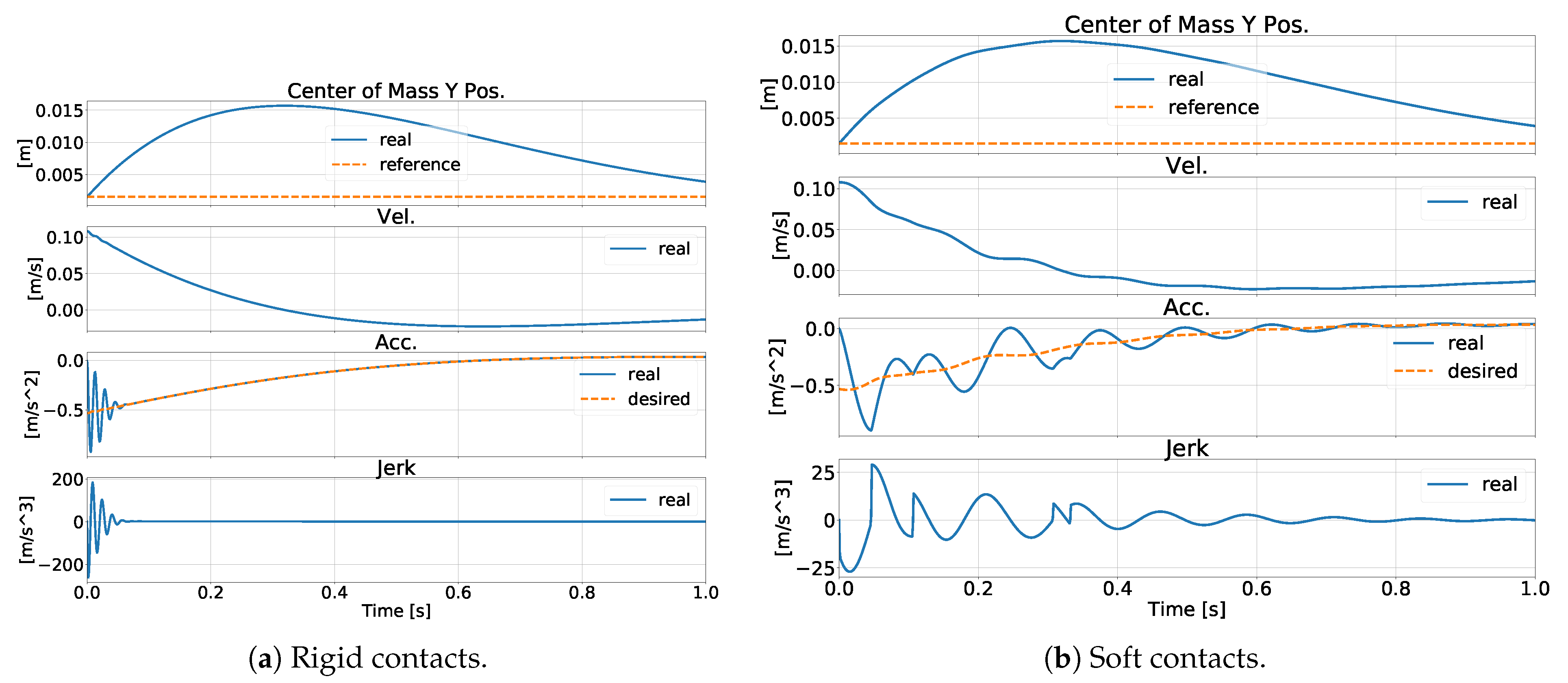
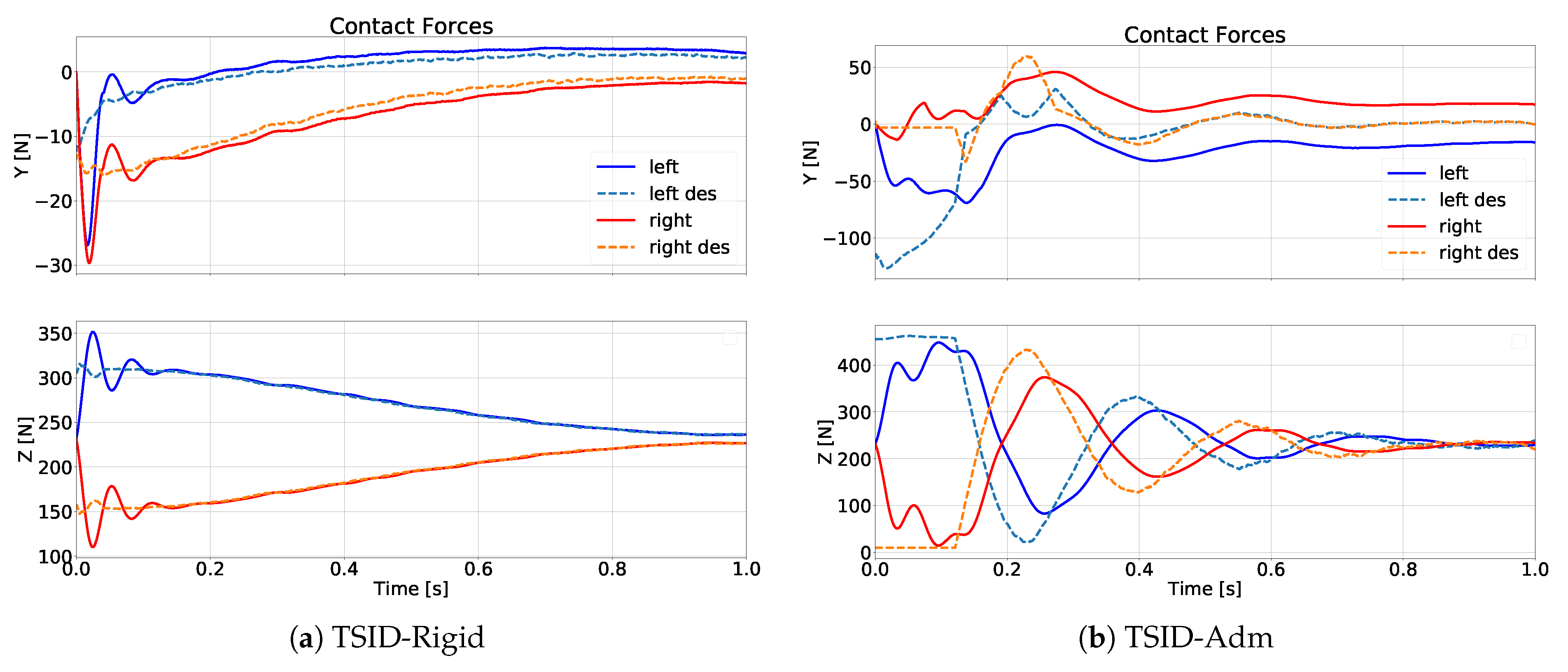
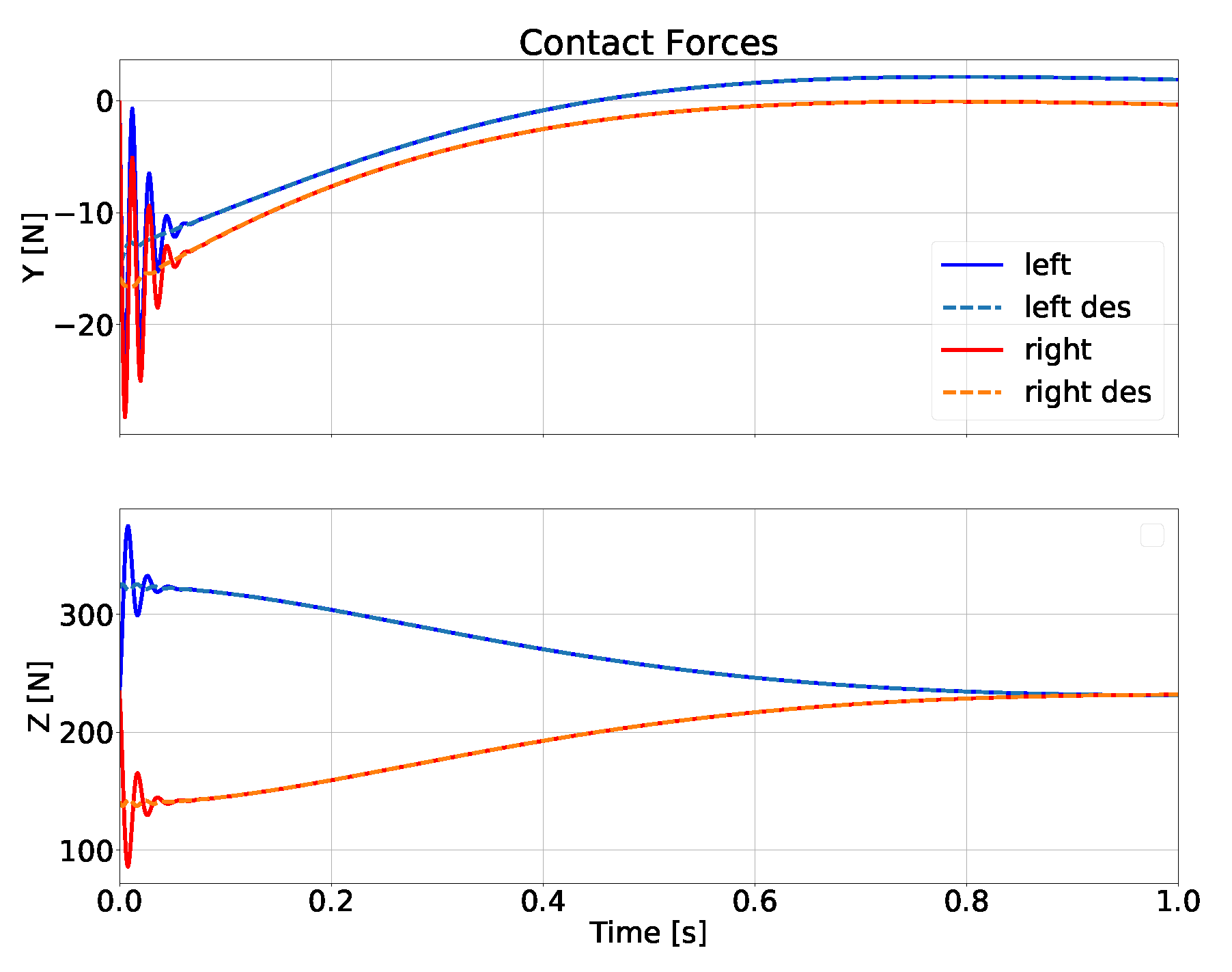
6.4. Test A: TSID-Rigid

We have tested TSID-Rigid on both rigid and soft contacts. Figure 2 shows the CoM trajectories obtained with noiseless simulation. With rigid contacts the controller regulates well the CoM position. Even the CoM velocity is smooth, but looking at the CoM jerk/snap we can see high-frequency oscillations at the beginning of the motion. For soft contacts, even though the system is still stable, performance has deteriorated. We can still see high CoM jerk/snap, which is undesirable, but since this time the oscillations last longer, they are also visible in the CoM velocity. Moreover, with rigid contacts the system remained stable for all gains, but this was not the case with soft contacts, where most gains led to instability (more details in Test D). This clearly highlights the need for a different control strategy to deal with soft contacts.

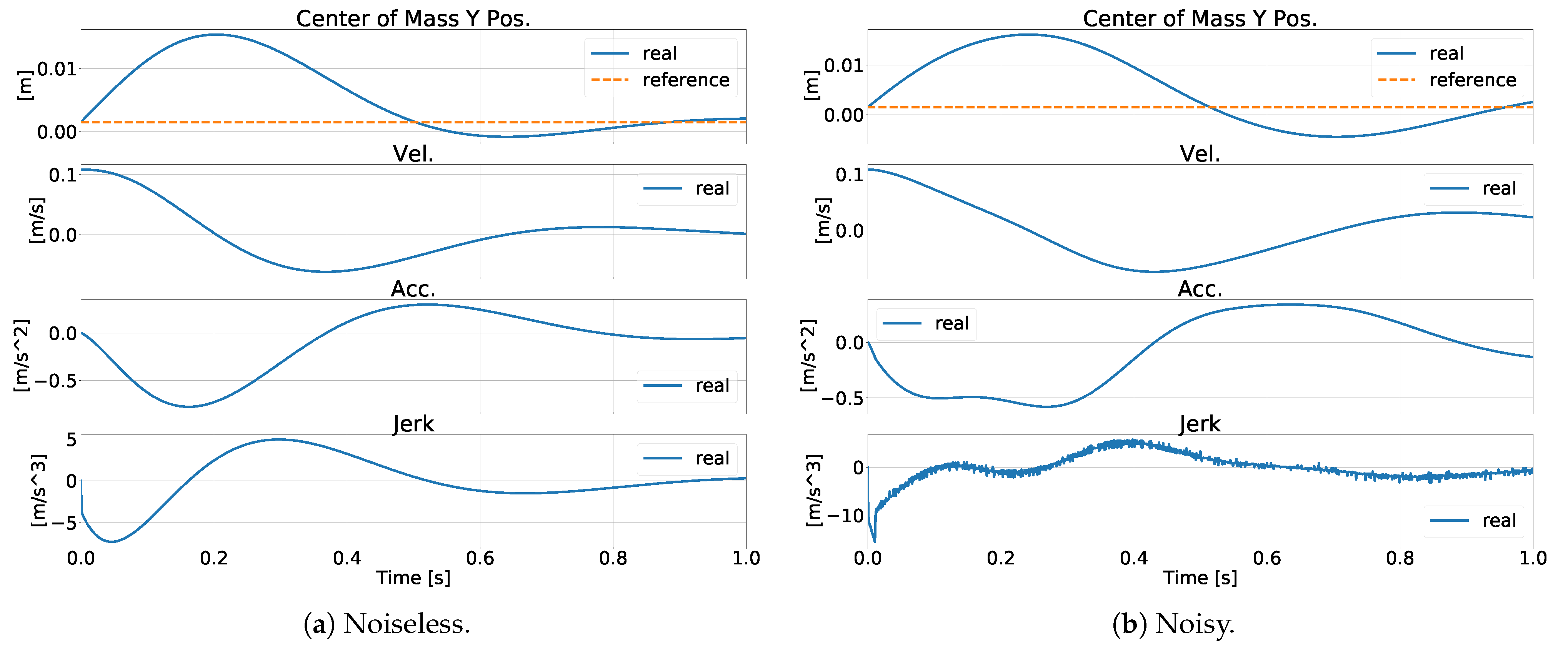
6.5. Test B: TSID-Flex-K and TSID-Adm

TSID-Flex-K and TSID-Adm have performed extremely well with soft contacts. Figure 3 shows that TSID-Flex-K gives smoother CoM trajectories than TSID-Rigid, e.g., for the noiseless case, peak CoM jerk is ≈7 ms${}^{-3}$ rather than ≈26 ms${}^{-3}$, while settling time is smaller. TSID-Adm has shown comparable performance on soft contacts, and Figure 4 shows that it has performed well also on medium contacts. TSID-Flex-K instead performed well on medium contacts only in the noiseless case, whereas it became unstable when noise was introduced. For hard contacts, TSID-Flex-K and TSID-Adm still performed well in noiseless simulations, but got unstable in the noisy case, as we will show in detail in Test D.

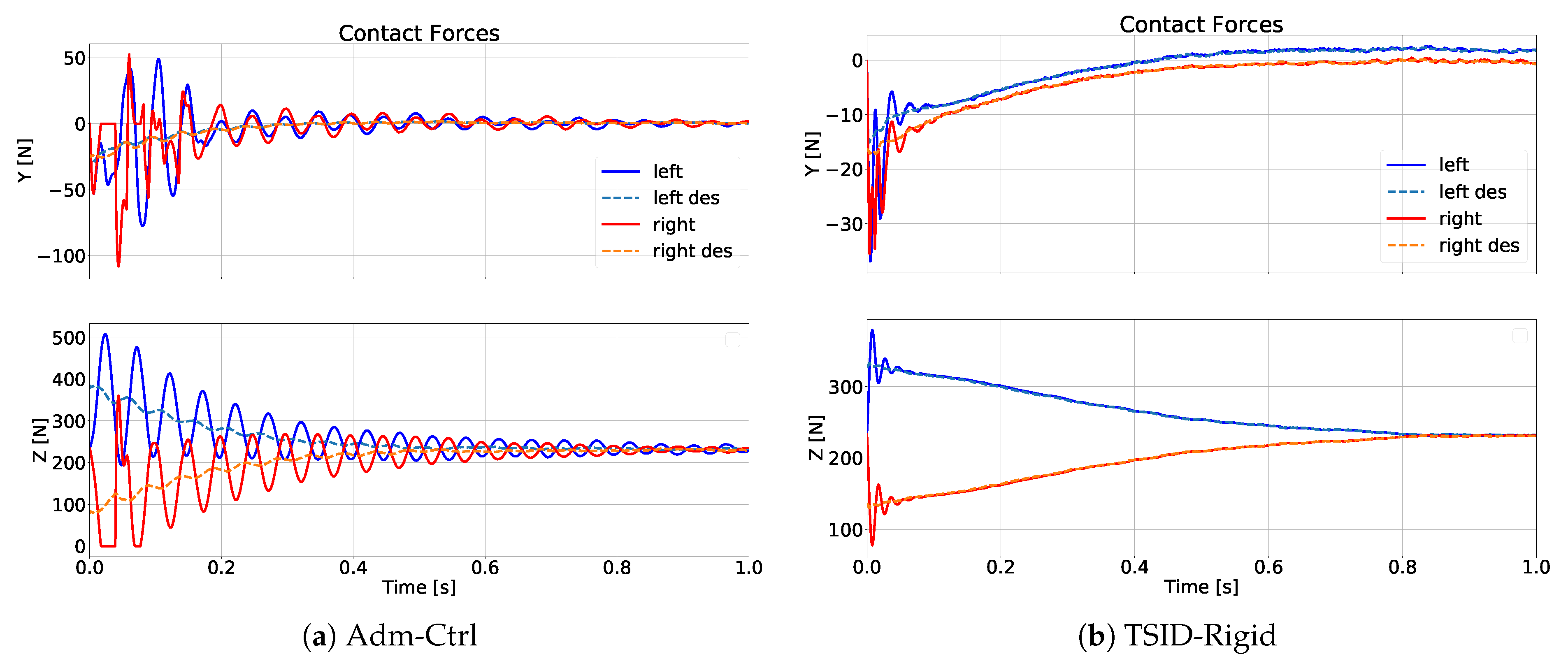
6.6. Test C: Adm-Ctrl

Adm-Ctrl has performed well across a large range of contact stiffnesses, as shown in Figure 5. Moreover, this controller has proven a remarkable robustness to noise, giving similar performance in the noiseless and noisy cases. The price to pay for this robustness seems to be a loss in performance, as measured by the cost function used in our gain-tuning procedure (more details in the following).

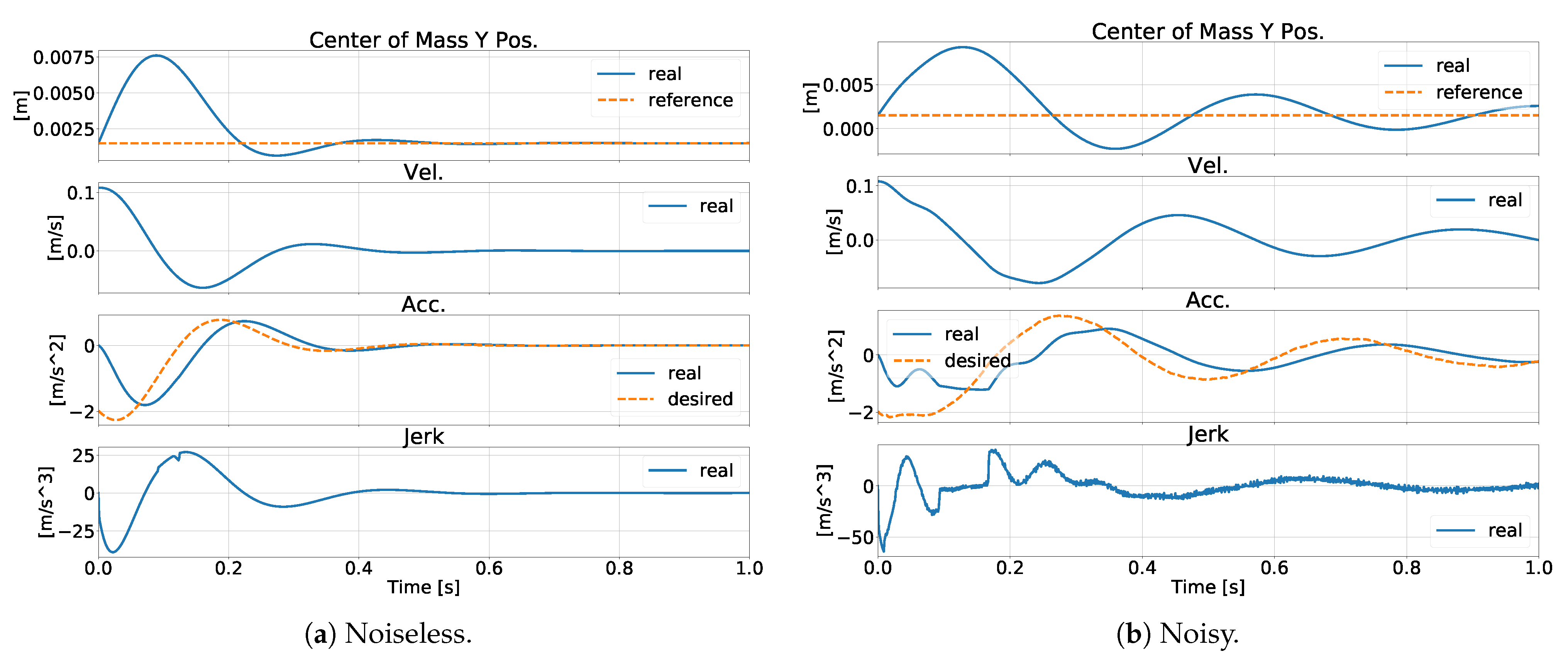
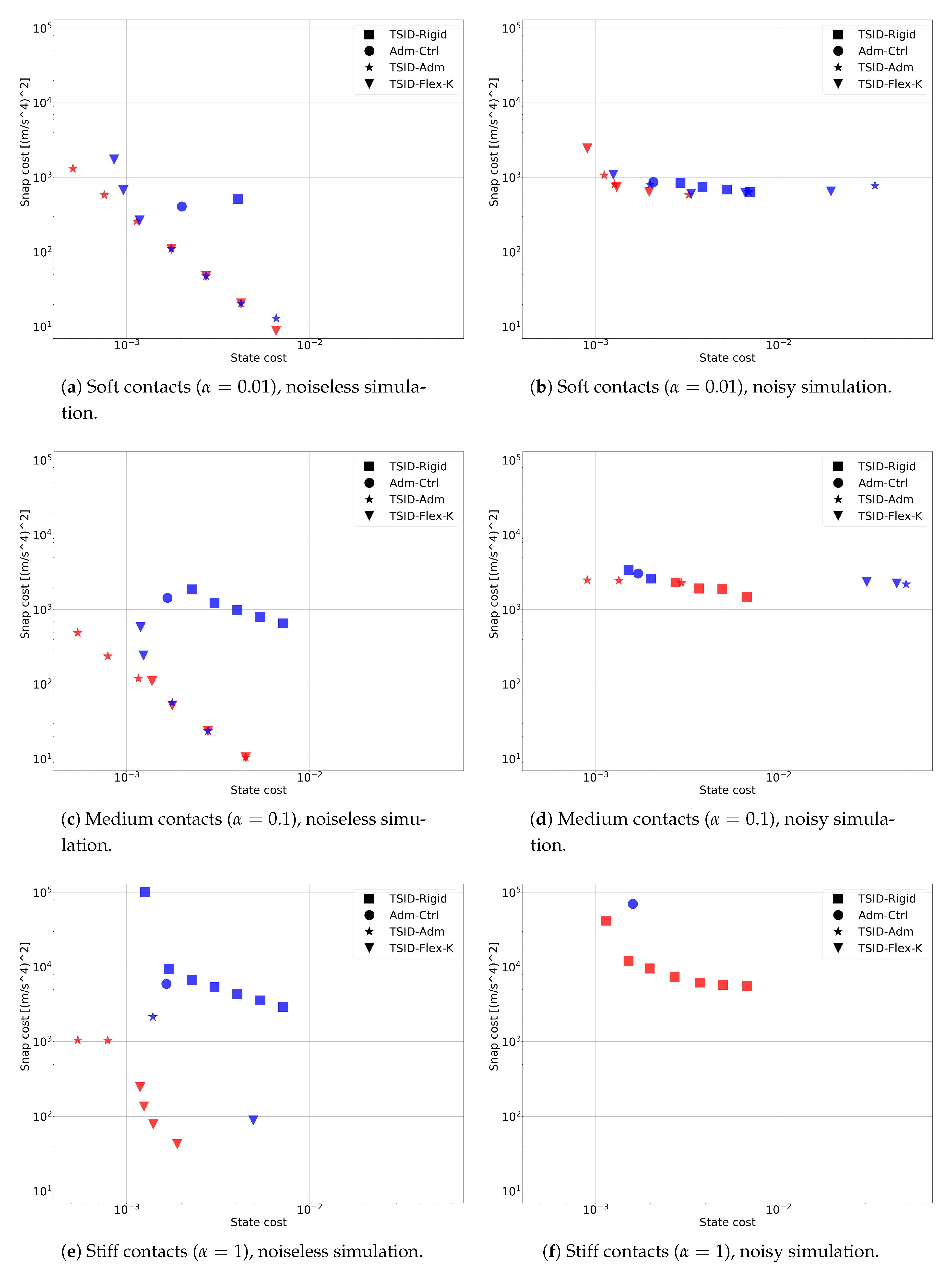
6.7. Test D: All Controllers

We now compare all four controllers, with different gains and contact stiffnesses. The results are summarized by Figure 6. Each plot shows the results of the four controllers for all the gain sets (1 for Adm-Ctrl and 7 for the other controllers), but for a specific contact stiffness (either soft, medium, or stiff) and a specific simulation type (either noiseless or noisy). The points missing in the plots are the ones that resulted in unstable simulations (i.e., NaN values). The plots highlight the trade-off between average CoM tracking error (x axis) and average CoM snap (y axis). The average CoM tracking error (“State cost”) measures how fast balance is recovered after an external perturbation, and it is defined as a weighted sum of CoM position and its first three derivatives along the simulation time:

$$\mathrm{State}\cos \mathrm{t}=\sum _{i=0}^N{y}_i^{\top }Q{y}_i,y\triangleq (c,\dot{c},\ddot{c},\stackrel{⃛}{c}),Q\triangleq \mathrm{diag}\left(\left[\begin{array}{c}1,0.1,{10}^{-3},{10}^{-6}\end{array}\right]\right)$$

(31)

The average CoM snap (“Snap cost”) quantifies both the CoM oscillations and the control effort, and it is defined as:

$$\mathrm{Snap}\cos \mathrm{t}=\sum _{i=0}^N{\left(c_i^{\left(4\right)}\right)}^{\top }{c}_i^{\left(4\right)}$$

(32)

6.7.1. Soft Contacts

In the noiseless simulations both TSID-Flex-K and TSID-Adm perform well, meaning that they achieve a good trade-off between state tracking and control effort. For lower feedback gains (i.e., higher position tracking errors) TSID-Flex-K and TSID-Adm achieve very similar performance, whereas for higher feedback gains they differ because of the ways in which they handle friction cones.

The unavoidable force tracking delay of admittance-control strategies is typically seen as an issue in the literature [3,8], because it clashes with the assumption of second-order dynamics. However, if we accept a fourth-order dynamics for our system, we can see that this delay is not at all incompatible with good CoM tracking (as long as gains are properly tuned), as shown for instance in Figure 7. The only downside of this delay is that it may lead TSID-Adm to violate friction cone constraints. Indeed, even though TSID-Adm constrains the desired forces inside friction cones, real forces may violate these constraints because of the tracking delay.

Adm-Ctrl performs reasonably well too, but less than TSID-Flex-K and TSID-Adm. On the contrary, TSID-Rigid is unstable for all the tested gain sets, except one, and even in this one case its performance is inferior to the other controllers (see Figure 2).

In the noisy simulations, things change remarkably. First, the performance of TSID-Flex-K and TSID-Adm gets worse, especially in terms of CoM snap, and in particular for lower feedback gains. Nonetheless, they remain the best controllers overall. Adm-Ctrl is only slightly affected by the introduction of noise, showing a remarkable robustness. Surprisingly, TSID-Rigid performs much better than in the noiseless case, showing a stable behavior with 3 gain sets, and getting a performance that is much closer to the Pareto front. To understand why, we have performed another test removing Coulomb friction (see Figure 8). This test shows that Coulomb friction was the cause of the improved stability of TSID-Rigid, and of much of the performance deterioration of the other controllers.

6.7.2. Medium Contacts

In the noiseless case TSID-Flex-K and TSID-Adm perform well, similarly to the soft-contact case. Adm-Ctrl also performs well, resulting in just a slightly higher CoM snap than for soft contacts. The main difference regarding the soft-contact case is that TSID-Rigid is stable for most gain sets (5 out of 7), even though it performs worse than the other controllers.

In the noisy simulations TSID-Flex-K becomes unstable for all feedback gains. TSID-Adm becomes unstable only for low feedback gains, but results in an increased CoM snap for higher gains. The performance of Adm-Ctrl and TSID-Rigid instead gets only slightly worse, showing a significant robustness. Out of the 7 Pareto-optimal points, 4 are associated with TSID-Rigid, and 3 to TSID-Adm.

Despite the performance of TSID-Rigid and TSID-Adm may seem comparable according to this plot, they are qualitatively different. Figure 9 shows one example of contact forces generated by the two approaches. TSID-Rigid generates fast-changing forces because it immediately applies the joint torques needed to generate the desired contact forces, and given the relatively high contact stiffness, these joint torques quickly result in the desired force change. TSID-Adm instead generates forces with larger oscillations, but with lower frequencies, which may be preferable on real hardware.

6.7.3. Stiff Contacts

In the noiseless case we can already observe a significant performance deterioration for TSID-Flex-K and TSID-Adm, which are unstable for many more gain sets (2 and 4 out of 7, respectively). Nonetheless, they remain the best controllers in this scenario. This deterioration is due to the control frequency, which is insufficient for this contact stiffness, so the sampling starts affecting stability and performance. For high contact stiffnesses, performance could be improved by designing and tuning controllers in the discrete-time domain.

TSID-Rigid and Adm-Ctrl perform similarly to the medium-contact case: stable, but with high CoM snap. In particular TSID-Rigid results in high-frequency oscillations of the contact forces (see Figure 10), which may excite unmodelled dynamics (e.g., link flexibility) in real systems.

In the noisy case TSID-Flex-K and TSID-Adm became unstable for all gains. We believe that this is due to the delay in the compensation of the estimated contact forces, which triggers instability. This delay is caused by the limited joint torque bandwidth and the joint Coulomb friction.

TSID-Rigid and Adm-Ctrl remained stable, but their performance is far from satisfactory. Figure 5 and Figure 11 show the obtained CoM and force trajectories, which are extremely oscillatory (especially for Adm-Ctrl) and are thus unlikely to work on real hardware.

The interested reader is invited to watch the accompanying video for more details about the simulation results.

7. Conclusions

This paper presented two novel control methods for balancing a legged robot on visco-elastic contacts: TSID-Flex-K and TSID-Adm. To ensure a fair comparison between novel and state-of-the-art methods we have used a unified gain-tuning procedure (except for Adm-Ctrl, which we have tuned by hand). We have performed several tests in simulation using a simple 4-DoF robot.

The presented results depict a broad picture of performance for 4 controllers, across 3 contact stiffnesses and 7 gain sets each (except for Adm-Ctrl, for which we have tested only one gain set). We highlight here the main pros and cons of each controller, which are also summarized in

Table 5. Summary of main features of each controller.

PROS	CONS
TSID-Flex-K and TSID-Adm
• Easy to tune (unified pos-force feedback).	• Need high frequency for hard contacts.
• Best for soft/medium contact.	• Unstable for hard contact with noise.
TSID-Rigid
• Ok for hard/medium contacts.	• Unstable for soft contacts.
• Easy to tune (assuming perfect joint torque tracking).	• Undesired oscillations (no force feedback).
Adm-Ctrl
• Always stable.	• Hard to tune/analyze.
• Good for soft contacts.	• Never the best.

.

The novel controllers presented in this paper (TSID-Flex-K and TSID-Adm) perform well for soft contacts, reasonably well for medium contacts, but they have showed instability for stiff contacts and noisy simulations.

TSID-Rigid has unsurprisingly shown the opposite trend, getting unstable for soft contacts (even though it was able to regain stability when introducing joint Coulomb friction), but then becoming more and more competitive as the contact stiffness increased. This is actually reasonable because the higher the contact stiffness, the more the system behaves as if contacts were rigid, which is a key assumption in TSID-Rigid.

One of the main advantages of the novel controllers is their ease of gain tuning, which allows for a unified tuning of force and position feedback gains (as acceleration/jerk gains can be seen as force gains). However, the novel controllers have demonstrated a remarkable sensitivity to uncertainties. We believe that this is due to the attempt to compensate for the contact forces, which are rapidly changing (especially for stiff contacts), thus easily leading to destabilizing compensation errors. This makes these methods sensitive to low control frequencies and actuation delays, such as the ones introduced by limited joint torques bandwidth and joint Coulomb friction.

Adm-Ctrl has been the only controller that was always stable, making it the most robust of them all. Despite its superior robustness, in no condition Adm-Ctrl has outperformed all the other controllers. Moreover, its gain tuning remains a heuristic procedure, and its convergence properties are not yet clearly understood. All of this makes this controller hard to use in practice, highlighting the need for more work on this subject.

Overall, the case of stiff contacts was the hardest for the tested controllers: only TSID-Rigid and Adm-Ctrl remained stable, but they resulted in oscillatory trajectories, which are (at best) unpleasant on real hardware. These oscillations are due to the small contact damping, which combined with the high contact stiffness makes it hard for the controller to damp the high-frequency force oscillations.

Finally, these results show that controllers that are well supported by theoretical results and perform exquisitely in ideal conditions, can then fail miserably in realistic simulations. Thus, working on robustness issues seems paramount for future work.

We believe that the subject of balance control on visco-elastic contacts still requires investigation. We are especially interested in improving the robustness of the proposed controllers, in the hope to find a better trade-off between performance and robustness. Another interesting direction could be to understand better the theoretical properties of Adm-Ctrl, which has clearly showed great robustness in our tests, but it remains unclear whether these capabilities can somehow be guaranteed in general.

References

1. Wieber, P.B.; Tedrake, R.; Kuindersma, S. Modeling and Control of Legged Robots. In Handbook of Robotics, 2nd ed.; Siciliano, B., Oussama, K., Eds.; Springer: Berlin/Heidelberg, Germany, 2015; Chapter 48. [Google Scholar]
2. Boaventura, T.; Semini, C.; Buchli, J.; Frigerio, M.; Focchi, M.; Caldwell, D.G. Dynamic torque control of a hydraulic quadruped robot. In Proceedings of the 2012 IEEE International Conference on Robotics and Automation, Saint Paul, MI, USA, 14–18 May 2012; pp. 1889–1894. [Google Scholar]
3. Englsberger, J.; Ott, C.; Albu-Schäffer, A. Three-Dimensional Bipedal Walking Control Based on Divergent Component of Motion. IEEE Trans. Robot. 2015, 31, 355–368. [Google Scholar] [CrossRef]
4. Herzog, A.; Rotella, N.; Mason, S.; Grimminger, F.; Schaal, S.; Righetti, L. Momentum control with hierarchical inverse dynamics on a torque-controlled humanoid. Auton. Robot. 2016, 40, 473–491. [Google Scholar] [CrossRef] [Green Version]
5. Lim, H.O.; Setiawan, S.A.; Takanishi, A. Balance and impedance control for biped humanoid robot locomotion. In Proceedings of the IEEE International Conference on Intelligent Robots and Systems, Maui, HI, USA, 29 October–3 November 2001; Volume 1, pp. 494–499. [Google Scholar]
6. Nava, G.; Romano, F.; Nori, F.; Pucci, D. Stability Analysis and Design of Momentum-based Controllers for Humanoid Robots. In Proceedings of the IEEE/RSJ International Conference on Intelligent Robots and Systems (IROS), Deajeon, Korea, 9–14 October 2016. [Google Scholar]
7. Takenaka, T.; Matsumoto, T.; Yoshiike, T.; Hasegawa, T.; Shirokura, S.; Kaneko, H.; Orita, A. Real time motion generation and control for biped robot-4 th report: Integrated balance control. In Proceedings of the IEEE/RSJ International Conference on Intelligent Robots and Systems, St. Louis, MO, USA, 11–15 October 2009; pp. 1601–1608. [Google Scholar]
8. Kajita, S.; Morisawa, M.; Miura, K.; Nakaoka, S.; Harada, K.; Kaneko, K.; Kanehiro, F.; Yokoi, K. Biped walking stabilization based on linear inverted pendulum tracking. In Proceedings of the IEEE/RSJ International Conference on Intelligent Robots and Systems (IROS), Taipei, Taiwan, 18–22 October 2010; pp. 4489–4496. [Google Scholar]
9. Li, Z.; Zhou, C.; Zhu, Q.; Xiong, R. Humanoid Balancing Behavior Featured by Underactuated Foot Motion. IEEE Trans. Robot. 2017, 33, 298–312. [Google Scholar] [CrossRef]
10. Reher, J.; Cousineau, E.A.; Hereid, A.; Hubicki, C.M.; Ames, A.D. Realizing dynamic and efficient bipedal locomotion on the humanoid robot DURUS. In Proceedings of the IEEE International Conference on Robotics and Automation, Stockholm, Sweden, 16–21 May 2016; pp. 1794–1801. [Google Scholar]
11. Henze, B.; Roa, M.A.; Ott, C. Passivity-based whole-body balancing for torque-conrolled humanoid robots in multi-contact scenarios. Int. J. Robot. Res. 2016, 35, 1522–1543. [Google Scholar] [CrossRef]
12. Azad, M.; Mistry, M.N. Balance control strategy for legged robots with compliant contacts. In Proceedings of the IEEE International Conference on Robotics and Automation, Seattle, WA, USA, 26–30 May 2015; pp. 4391–4396. [Google Scholar]
13. Fahmi, S.; Mastalli, C.; Focchi, M.; Semini, C. Passive Whole-Body Control for Quadruped Robots: Experimental Validation over Challenging Terrain. IEEE Robot. Autom. Lett. 2019, 4, 2553–2560. [Google Scholar] [CrossRef] [Green Version]
14. Fahmi, S.; Focchi, M.; Radulescu, A.; Fink, G.; Barasuol, V.; Semini, C. STANCE: Locomotion Adaptation over Soft Terrain. IEEE Trans. Robot. 2020, 36, 443–457. [Google Scholar] [CrossRef]
15. Orin, D.E.; Goswami, A.; Lee, S.H. Centroidal dynamics of a humanoid robot. Auton. Robot. 2013, 35, 161–176. [Google Scholar] [CrossRef]
16. Hirai, K.; Hirose, M.; Haikawa, Y.; Takenaka, T. The development of Honda humanoid robot. In Proceedings of the IEEE International Conference on Robotics and Automation, Leuven, Belgium, 16–20 May 1998. [Google Scholar]
17. Caron, S.; Kheddar, A.; Tempier, O. Stair Climbing Stabilization of the HRP-4 Humanoid Robot using Whole-body Admittance Control. arXiv 2018, arXiv:1809.07073. [Google Scholar]
18. Saccon, A.; Traversaro, S.; Nori, F.; Nijmeijer, H. On Centroidal Dynamics and Integrability of Average Angular Velocity. IEEE Robot. Autom. Lett. 2017, 2, 943–950. [Google Scholar] [CrossRef] [Green Version]
19. Del Prete, A. Joint Position and Velocity Bounds in Discrete-Time Acceleration/ Torque Control of Robot Manipulators. IEEE Robot. Autom. Lett. 2018, 3, 281–288. [Google Scholar] [CrossRef] [Green Version]
20. Kaneko, K.; Kanehiro, F. Design of prototype humanoid robotics platform for HRP. In Proceedings of the IEEE/RSJ International Conference on Intelligent Robots and Systems (IROS), Lausanne, Switzerland, 30 September–4 October 2002. [Google Scholar]
21. Dallali, H.; Medrano-Cerda, G.A.; Focchi, M.; Boaventura, T.; Frigerio, M.; Semini, C.; Buchli, J.; Caldwell, D.G. On the use of positive feedback for improved torque control. Control. Theory Technol. 2015, 13, 266–285. [Google Scholar] [CrossRef]
22. Paine, N.; Oh, S.; Sentis, L. Design and Control Considerations for High-Performance Series Elastic Actuators. IEEE/ASME Trans. Mechatron. 2014, 19, 1080–1091. [Google Scholar] [CrossRef] [Green Version]
23. Rotella, N.; Herzog, A.; Schaal, S.; Righetti, L. Humanoid momentum estimation using sensed contact wrenches. In Proceedings of the IEEE-RAS International Conference on Humanoid Robots, Seoul, Korea, 3–5 November 2015; pp. 556–563. [Google Scholar]
24. Flayols, T.; Del Prete, A.; Wensing, P.; Mifsud, A.; Benallegue, M.; Stasse, O. Experimental Evaluation of Simple Estimators for Humanoid Robots. In Proceedings of the IEEE International Conference on Humanoid Robots (Humanoids), Birmingham, UK, 15–17 November 2017; pp. 889–895. [Google Scholar]
Figure 1. 2d biped robot used for simulations.
Applsci 11 00353 g001
Figure 2. Test A: performance of TSID-Rigid in noiseless simulation.
Applsci 11 00353 g002
Figure 3. Test B: CoM trajectory obtained with TSID-Flex-K, and soft contacts.
Applsci 11 00353 g003
Figure 4. Test B: CoM trajectory obtained with TSID-Adm, and medium contacts.
Applsci 11 00353 g004
Figure 5. Test C: CoM trajectory obtained with Adm-Ctrl in noisy simulations.
Applsci 11 00353 g005
Figure 6. Summary of all results. Pareto-optimal tests are depicted in red, while the others in blue.
Applsci 11 00353 g006
Figure 7. TSID-Adm, soft contacts ( α = 0.01 ), noiseless simulation and low feedback gains ( w u = 10 6 ). CoM tracking is good despite the significant delay in force tracking.
Applsci 11 00353 g007
Figure 8. Results for soft contacts ( α = 0.01 ) and noisy simulation, but without Coulomb friction. Coulomb friction has a detrimental effect to the performance of TSID-Flex-K and TSID-Adm, while it helps stabilizing TSID-Rigid.
Applsci 11 00353 g008
Figure 9. Comparison between contact forces given by TSID-Rigid and TSID-Adm for medium contacts, noisy simulations.
Applsci 11 00353 g009
Figure 10. Contact force generated by TSID-Rigid with stiff contacts, noiseless simulation.
Applsci 11 00353 g010
Figure 11. Stiff contacts, noisy simulation.
Applsci 11 00353 g011