Day-Ahead Optimization of Prosumer Considering Battery Depreciation and Weather Prediction for Renewable Energy Sources


Abstract
1. Introduction
2. Overall Description of the Model
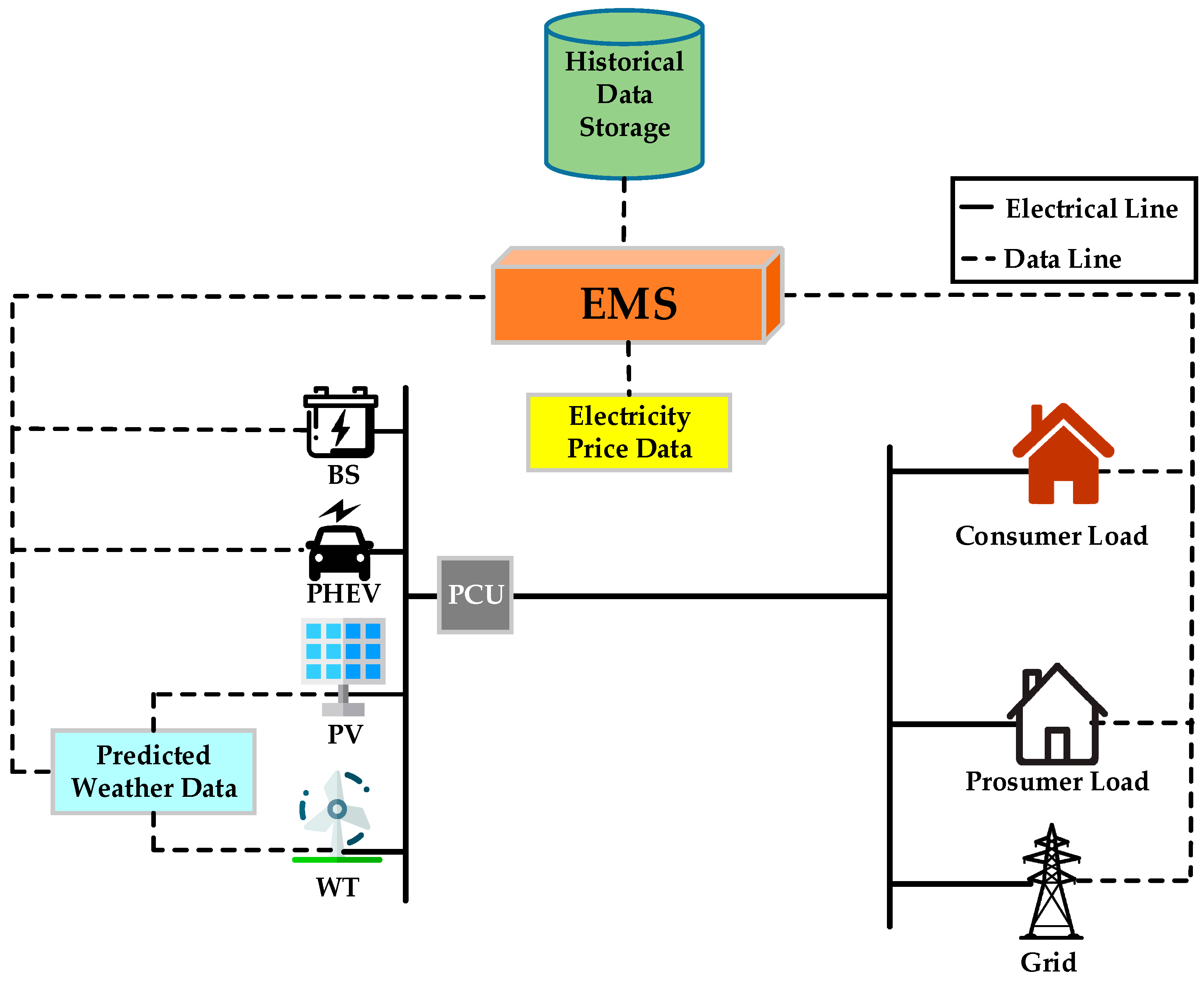
2.1. System Architecture
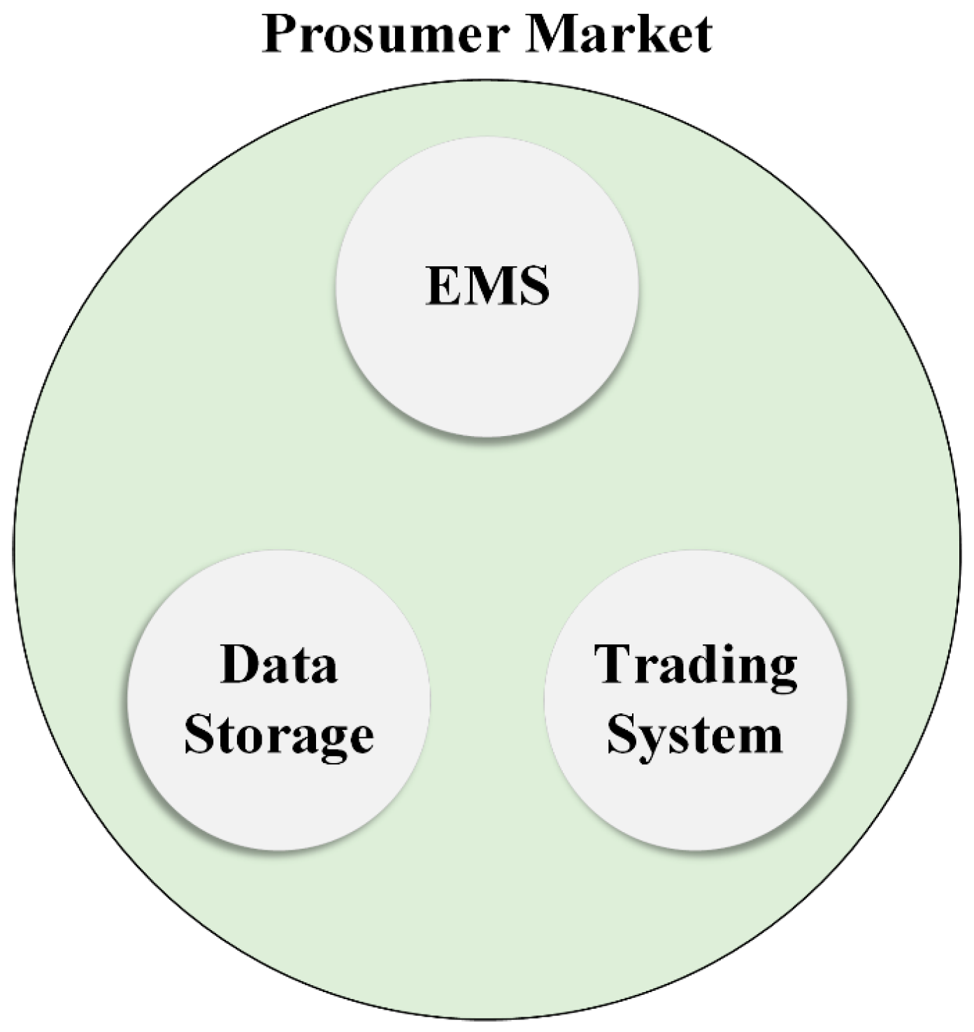
2.2. The Role of Prosumer
3. Methodology
3.1. Mathematical Modeling of RESs
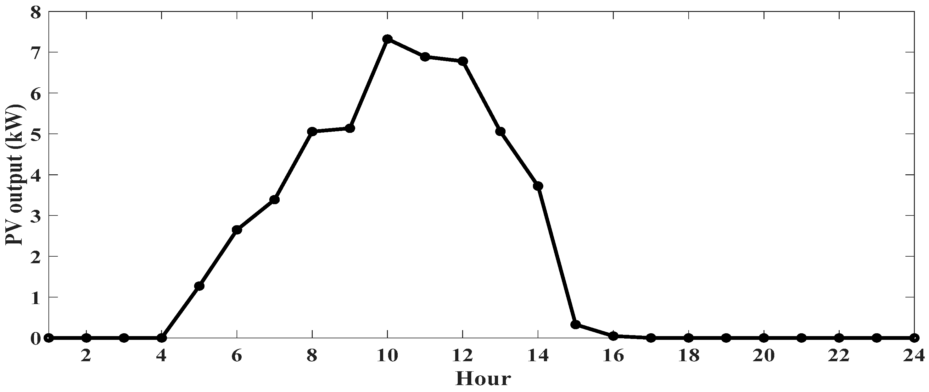
3.1.1. PV Unit
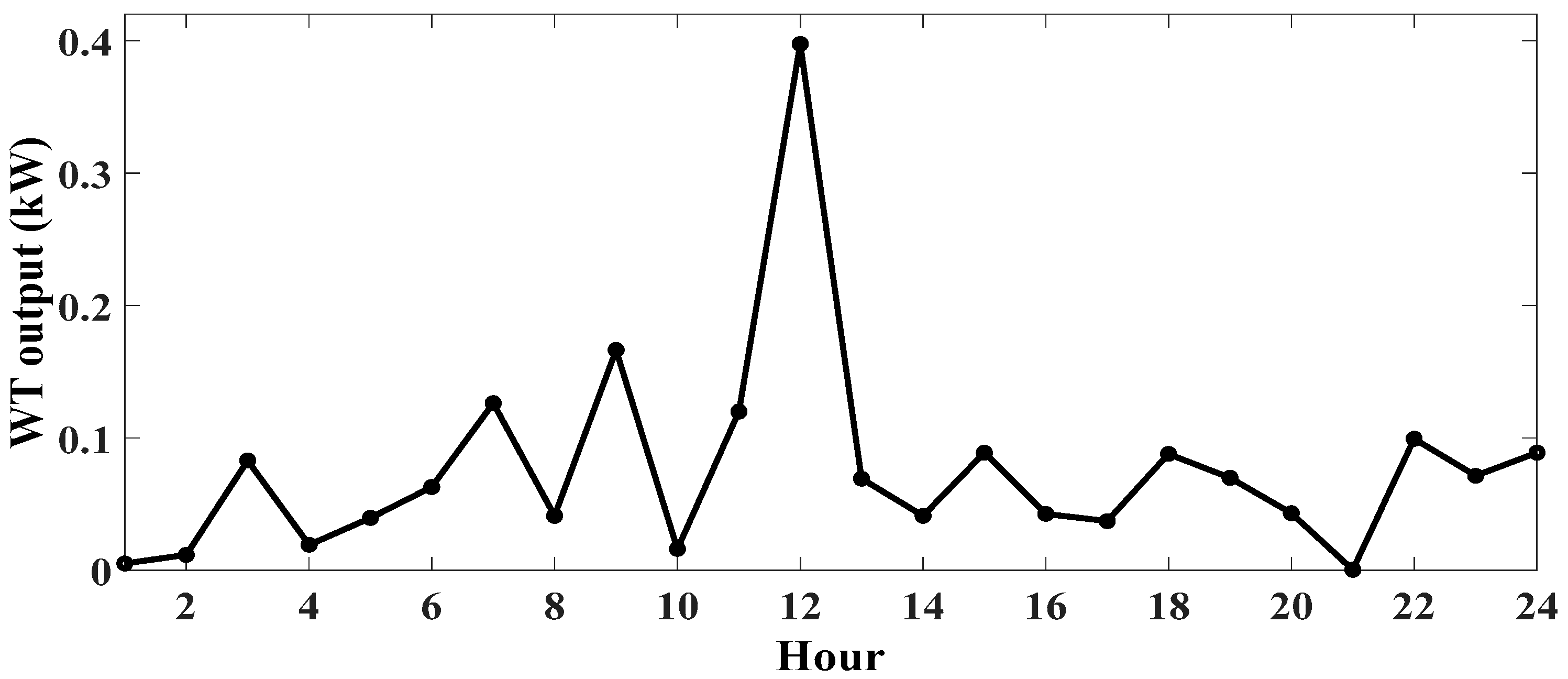
3.1.2. WT Unit
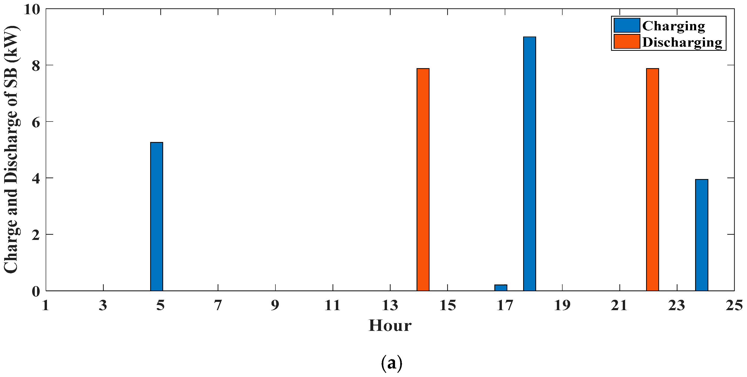
3.1.3. Energy Storage Systems
3.1.4. Depreciation of ESSs
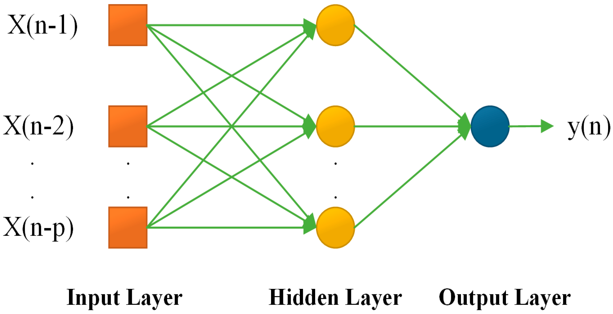
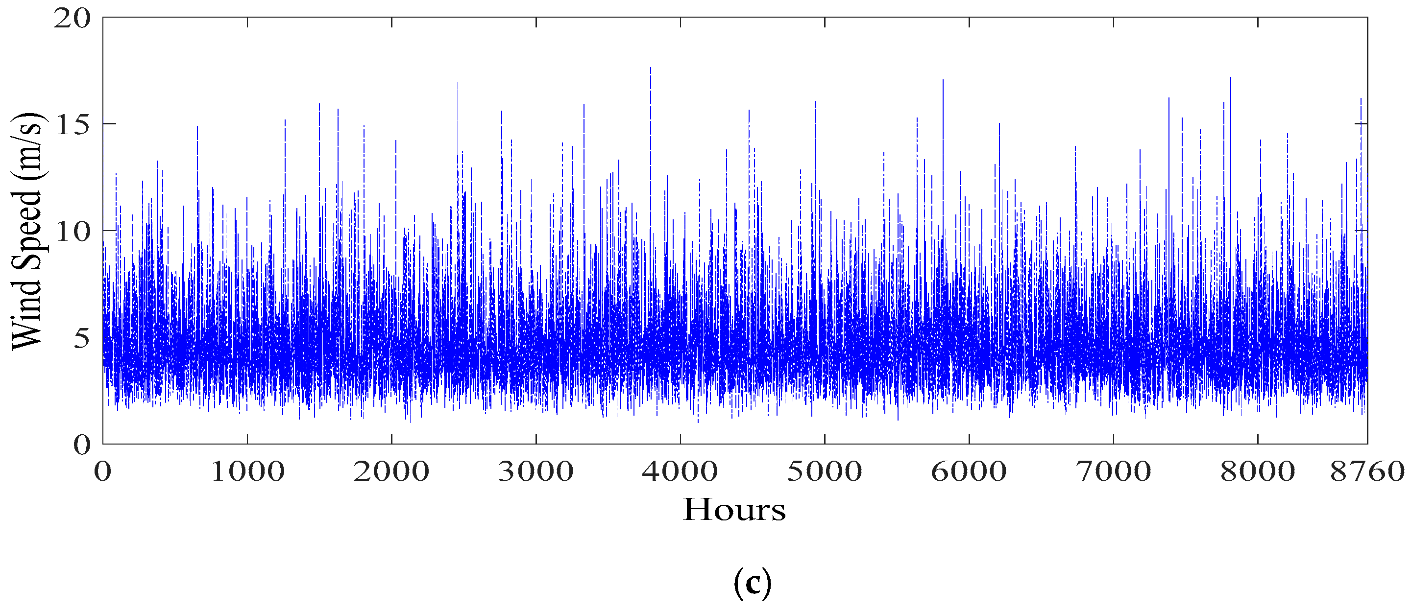
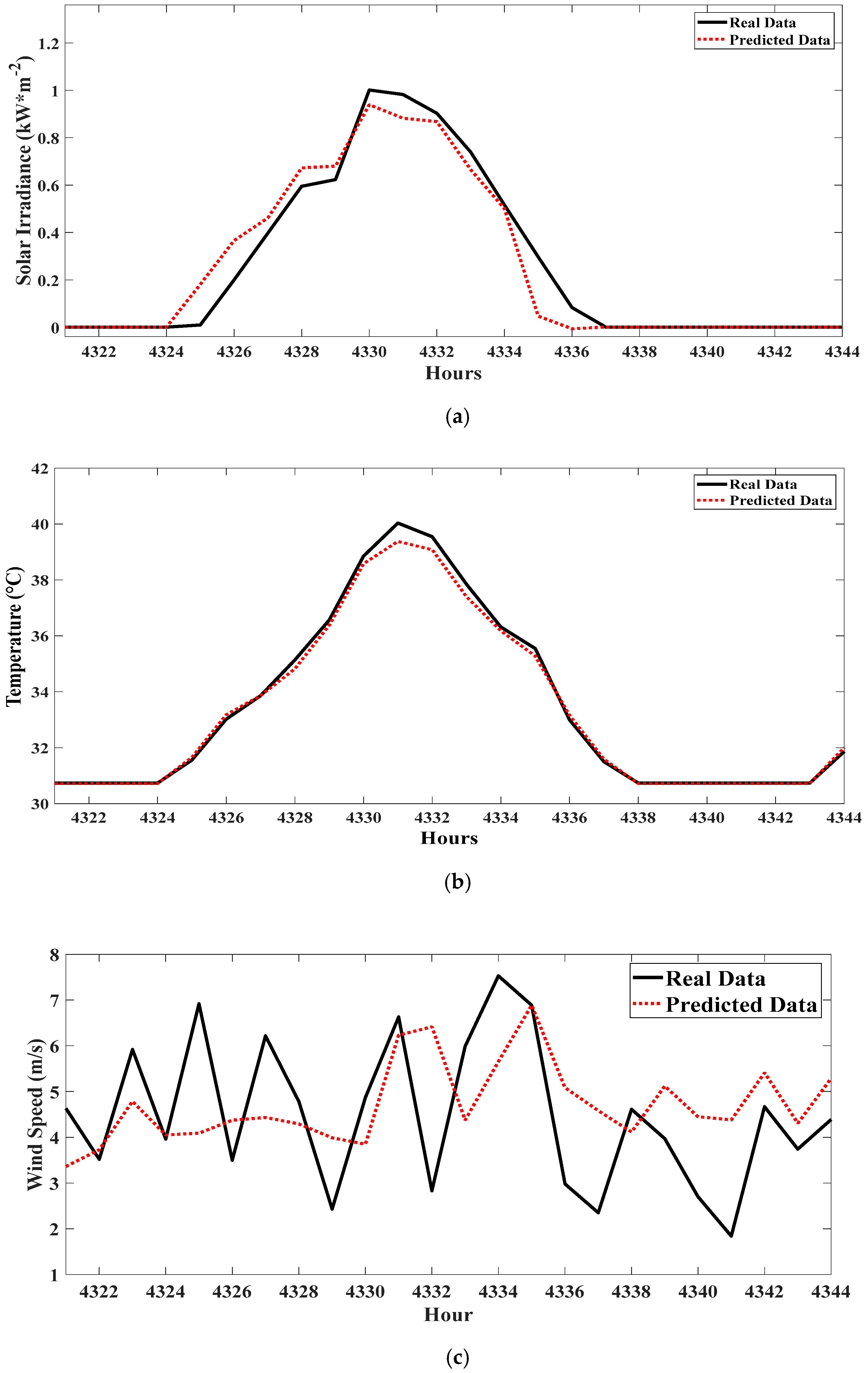
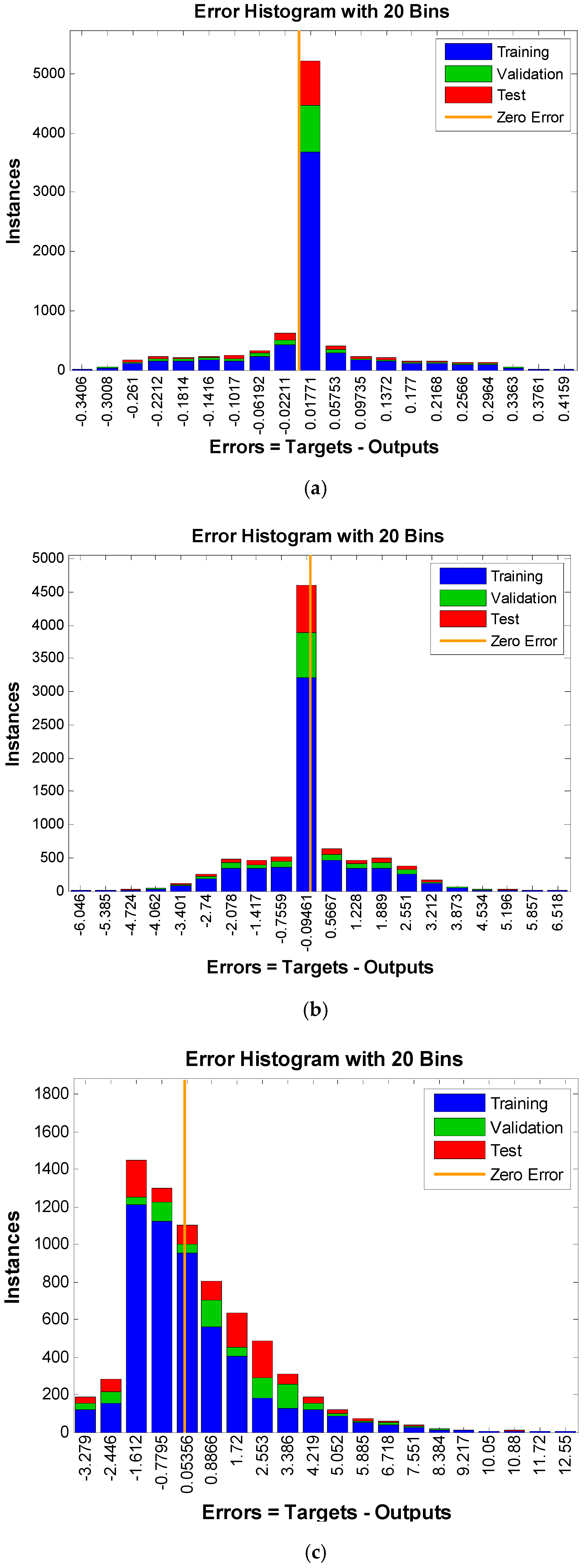
3.2. Predicting Weather Parameters Using Time Series FF-ANN
3.3. Optimization Modeling
4. Simulation Results and Discussion
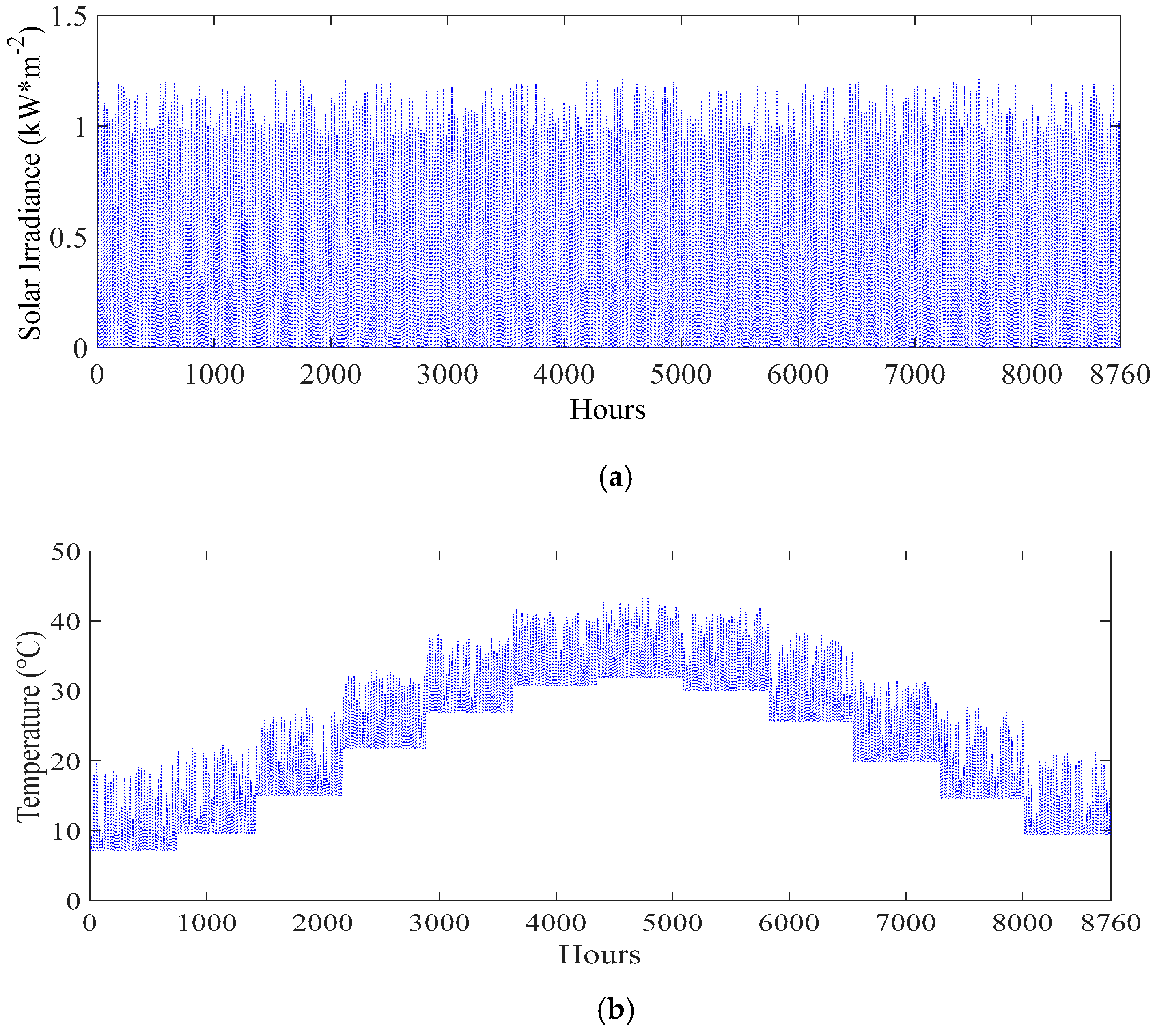
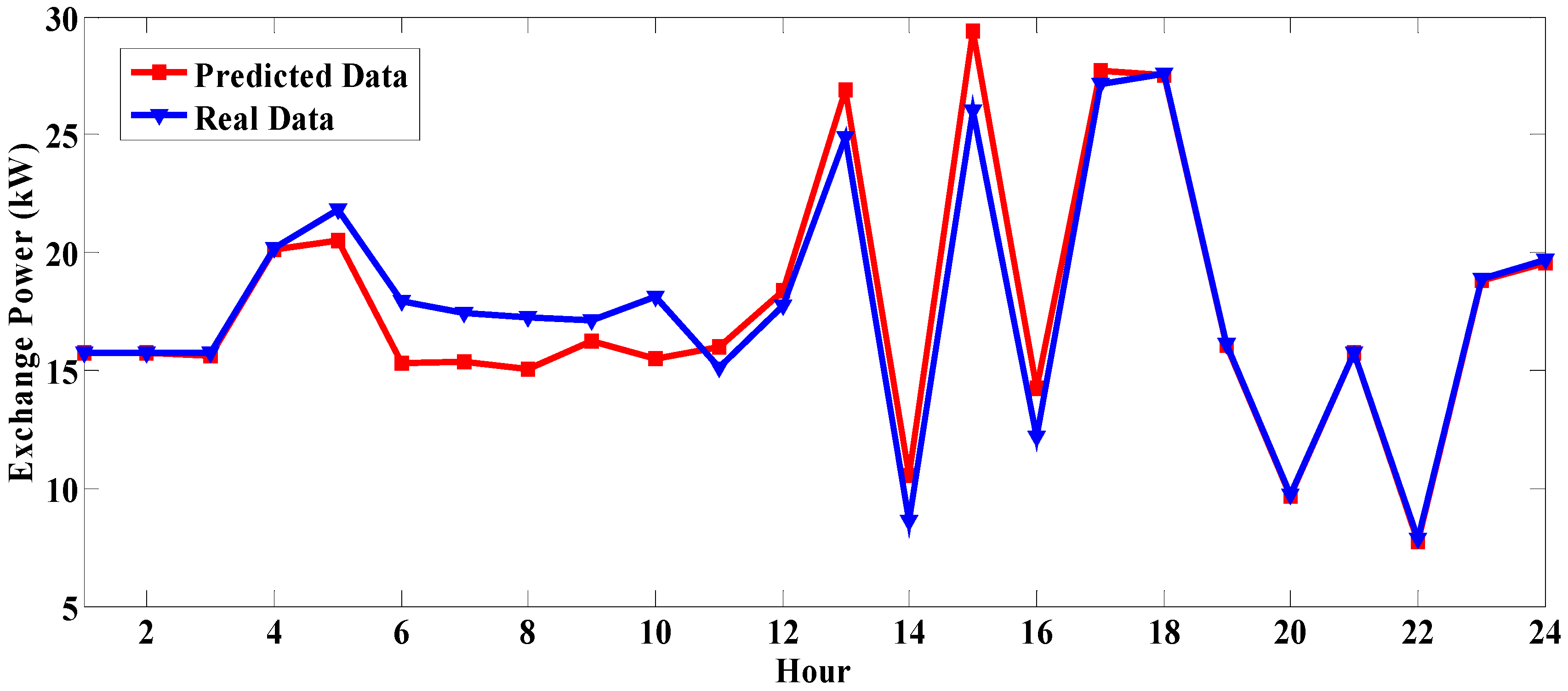
4.1. Prediction Results
4.2. Case Studies
- Case 1: Day-ahead scheduling of the prosumer considering predicted weather data.
- Case 2: Day-ahead scheduling of the prosumer considering ESSs depreciation cost and predicted weather data.
- Case 3: Day-ahead scheduling of the prosumer considering real weather data.
4.3. Results of Case Studies
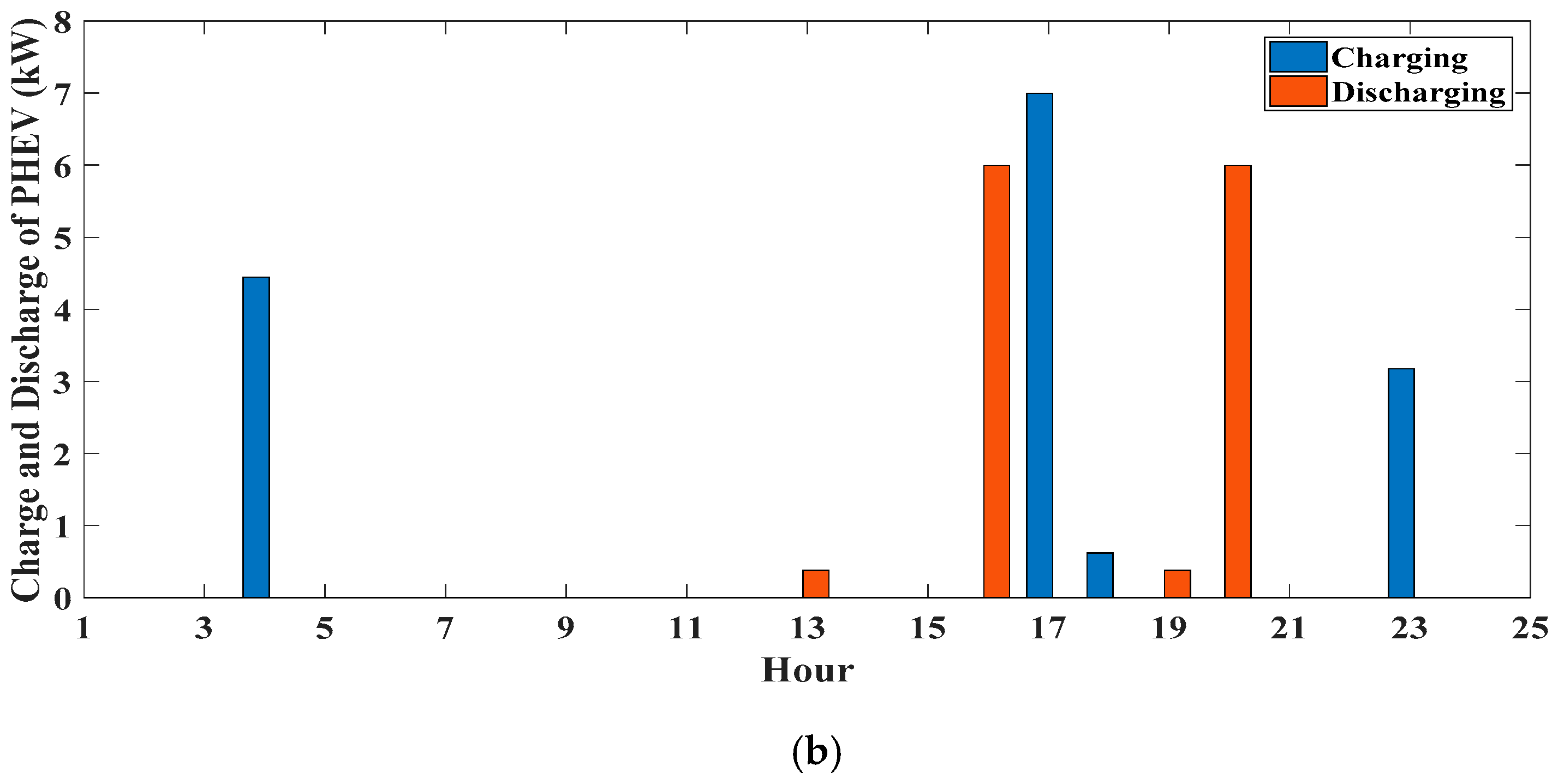
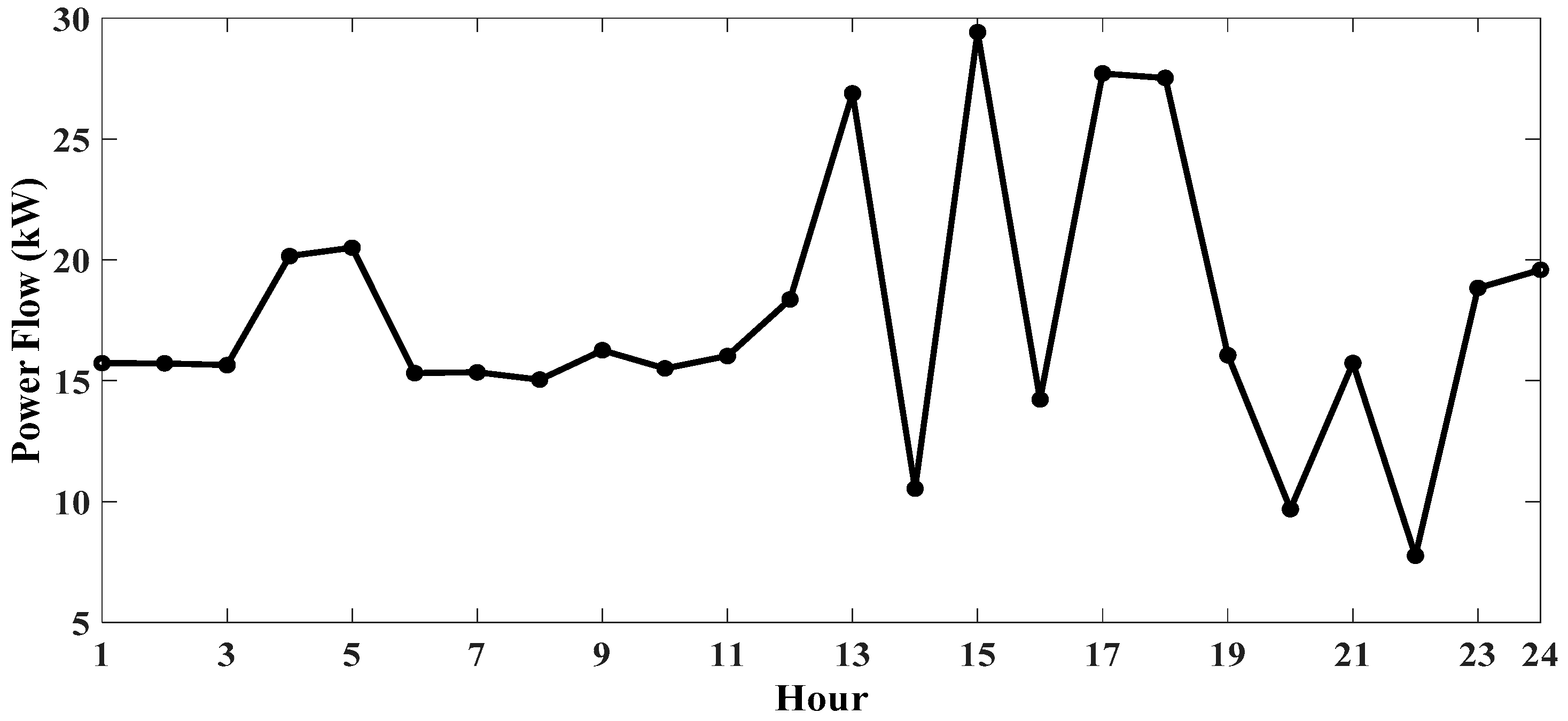
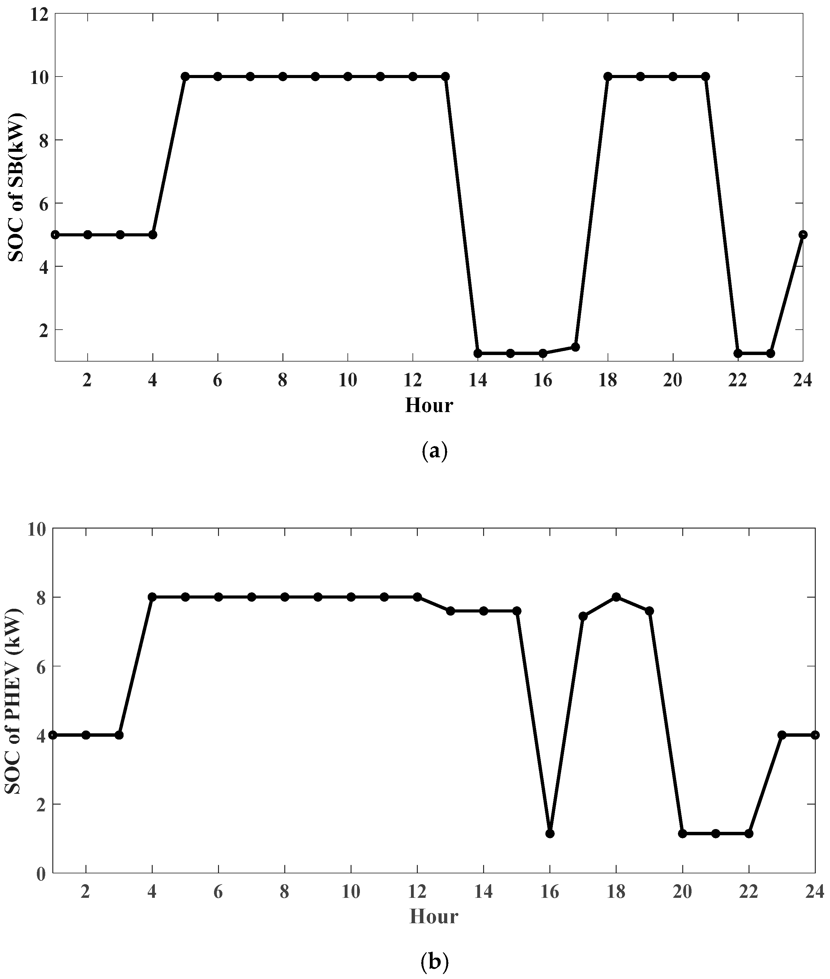
4.3.1. Case 1
4.3.2. Case 2
4.3.3. Case 3
5. Conclusions
Author Contributions
Funding
Conflicts of Interest
Nomenclature
| Parameters | |
| Initial ESS SOC (kWh) | |
| Final ESS SOC (kWh) | |
| Upper band of ESS SOC (kWh) | |
| Lower band of ESS SOC (kWh) | |
| Lower band of ESS charge (kWh) | |
| Upper band of ESS charge (kWh) | |
| Lower band of ESS discharge (kWh) | |
| Upper band of ESS discharge (kWh) | |
| Charge coefficient of ESS (%) | |
| Charge coefficient of ESS (%) | |
| Number installed PV modules | |
| Area of the module (m2) | |
| Replacement cost of SB ($) | |
| Lifetime of the SB (year) | |
| Square root of both ways of efficiency of the SB (%) | |
| Replacement cost of PHEV ($) | |
| Lifetime of the PHEV (year) | |
| Square root of both ways of efficiency of the PHEV (%) | |
| SB depreciation cost coefficient per kWh | |
| PHEV depreciation cost coefficient per kWh | |
| Rated efficiency of PV measured at referenced temperature (25 °C) | |
| Normal cell operation temperature (°C) | |
| Reference temperature (25 °C) | |
| Temperature coefficient for cell efficiency (0.004/°C) | |
| Cut-out speed (m/s) | |
| Cut-in speed (m/s) | |
| Wind speed at rated power (m/s) | |
| Upper bound of import power from grid (kWh) | |
| Power export limit to grid (kWh) | |
| Variables | |
| Efficiency of PV module (%) | |
| Hourly solar irradiance (kW×m−2) | |
| Hourly ambient temperature (°C) | |
| Hourly wind speed (V) | |
| Hourly electricity price ($) | |
| Charge power of ESS (kWh) | |
| Discharge power of ESS (kWh) | |
| Power flow from or to grid (kWh) | |
| Output power of PV (kWh) | |
| Output power of WT (kWh) | |
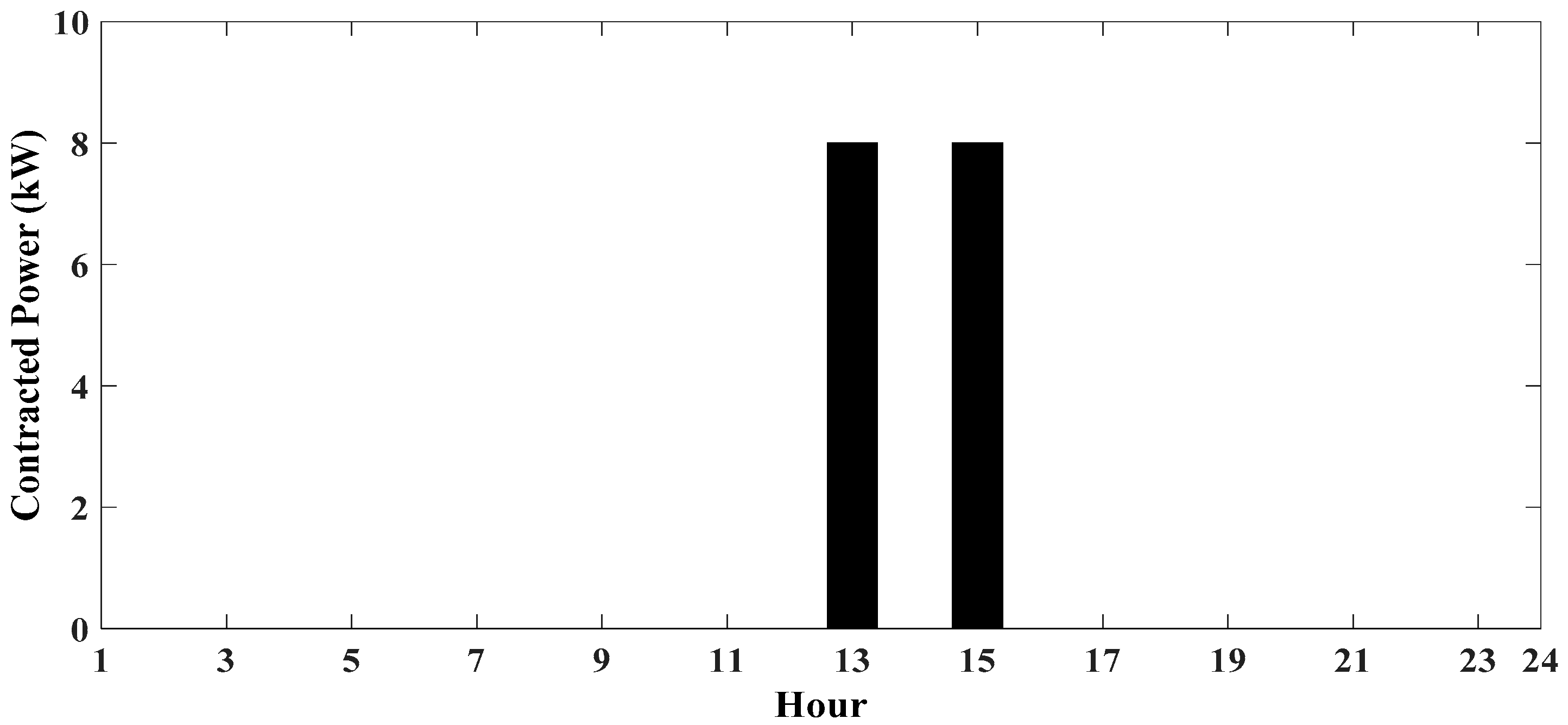
| Contracted power (kWh) | |
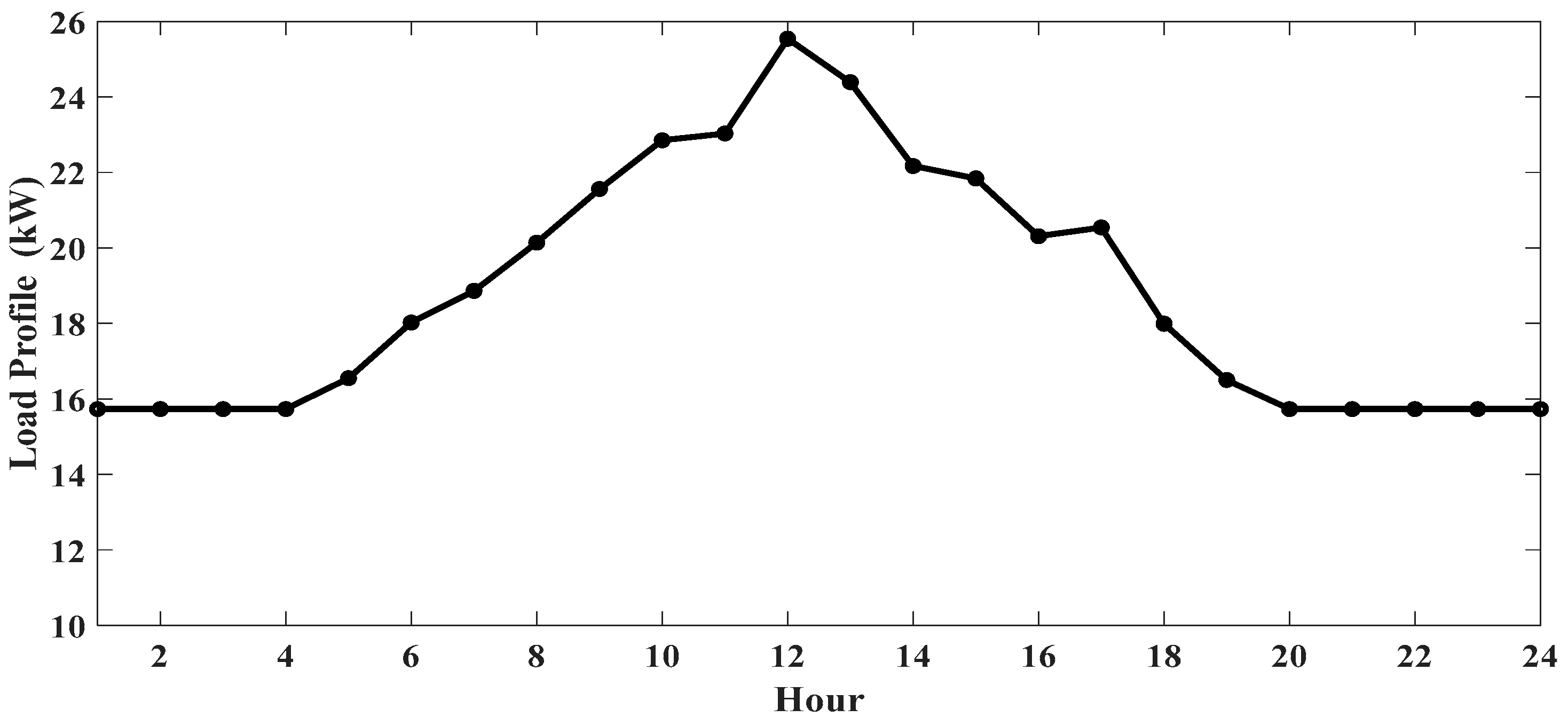
| Prosumer load profile (kWh) | |
| Minimum SB SOC at the end of the day (kWh) | |
| Minimum SOC of PHEV at the end of the day (kWh) | |
| SOC in each hour (kWh) | |
| Total EES depreciation cost ($) | |
| SB depreciation cost ($) | |
| PHEV depreciation cost ($) | |
| Original data value | |
| Normalized data value | |
| Minimum and maximum value of x | |
| [0,1] | |
| ESS charge binary variable | |
| ESS discharge binary variable | |
| Indices | |
| t | Index of time |
| d | Index of day |
| Abbreviations | |
| RES | Renewable Energy Source |
| SB | Stationary Battery |
| EV | Electric Vehicle |
| FEV | Fully Electric Vehicle |
| FCEV | Fuel Cell Electric Vehicle |
| PHEV | Plug-in Hybrid Electrical Vehicle |
| ESS | Energy Storage System |
| PV | Photovoltaic |
| WT | Wind Turbine |
| PCU | Power Conversion Unit |
| EMS | Energy Management System |
| ANN | Artificial Neural Network |
| FF | Feedforward |
| MLP | Multilayer Perceptron |
| DOD | Depth of Charge |
| SOC | State of Charge |
| MILP | Mixed-Integer Linear Programming |
| BP | Back Propagation |
| TOU | Time of Use |
| DR | Demand Response |
| DSO | Distribution System Operator |
References
- IEA-RETD (2014). Residental Prosumers–Drivers and Policy Options (RE-Prosumers). 2014. Available online: https://www.osti.gov/servlets/purl/1163237 (accessed on 12 July 2019).
- Faraji, J.; Babaei, M.; Bayati, N.; Hejazi, M.A. A Comparative Study between Traditional Backup Generator Systems and Renewable Energy Based Microgrids for Power Resilience Enhancement of a Local Clinic. Electronics 2019, 8, 1485. [Google Scholar] [CrossRef]
- Hosseinnezhad, V.; Shafie-Khah, M.; Siano, P.; Catalão, J.P.S. An Optimal Home Energy Management Paradigm with an Adaptive Neuro-Fuzzy Regulation. IEEE Access 2020, 8, 19614–19628. [Google Scholar] [CrossRef]
- Zia, M.F.; Elbouchikhi, E.; Benbouzid, M. Optimal operational planning of scalable DC microgrid with demand response, islanding, and battery degradation cost considerations. Appl. Energy 2019, 237, 695–707. [Google Scholar] [CrossRef]
- Abazari, A.; Dozein, M.G.; Monsef, H.; Wu, B. Wind turbine participation in micro-grid frequency control through self-tuning, adaptive fuzzy droop in de-loaded area. Iet Smart Grid 2019, 2, 301–308. [Google Scholar] [CrossRef]
- Heinisch, V.; Odenberger, M.; Göransson, L.; Johnsson, F. Prosumers in the Electricity System—Household vs. System Optimization of the Operation of Residential Photovoltaic Battery Systems. Front. Energy Res. 2019, 6. [Google Scholar] [CrossRef]
- Bae, D. E-mobility 시대의 에너지저장매체 선택 기준. ER20-047-N2611; KOSEN Report 2020. 2020. Available online: https://www.kosen21.org/info/kosenReport/reportView.do?articleSeq=REPORT_0000000001506 (accessed on 2 April 2020).
- Radan, P. Mitsubishi Outlander PHEV Unveiling in Iran. Available online: http://ariancapital.ir/mitsubishi-outlander-phev-unveiling-iran/ (accessed on 4 March 2020).
- Abazari, A.; Dozein, M.G.; Monsef, H. An optimal fuzzy-logic based frequency control strategy in a high wind penetrated power system. J. Frankl. Inst. 2018, 355, 6262–6285. [Google Scholar] [CrossRef]
- Zhang, F.; Meng, K.; Xu, Z.; Dong, Z.; Zhang, L.; Wan, C.; Liang, J. Battery ESS Planning for Wind Smoothing via Variable-Interval Reference Modulation and Self-Adaptive SOC Control Strategy. IEEE Trans. Sustain. Energy 2017, 8, 695–707. [Google Scholar] [CrossRef]
- Shim, J.W.; Verbič, G.; An, K.; Lee, J.H.; Hur, K. Decentralized operation of multiple energy storage systems: SOC management for frequency regulation. In Proceedings of the 2016 IEEE International Conference on Power System Technology (POWERCON), Wollongong, NSW, Australia, 28 September–1 October 2016; pp. 1–5. [Google Scholar]
- Xin, P.; Hanchen, X.; Chao, L.; Jie, S. Energy storage system control strategy in frequency regulation. In Proceedings of the 2016 IEEE International Conference on Automation Science and Engineering (CASE), Fort Worth, TX, USA, 21–25 August 2016; pp. 664–669. [Google Scholar]
- Liu, J.; Wen, J.; Yao, W.; Long, Y. Solution to short-term frequency response of wind farms by using energy storage systems. Iet Renew. Power Gener. 2016, 10, 669–678. [Google Scholar] [CrossRef]
- Abazari, A.; Dozein, M.G.; Monsef, H. A New Load Frequency Control Strategy for an AC Micro-grid: PSO-based Fuzzy Logic Controlling Approach. In Proceedings of the 2018 Smart Grid Conference (SGC), Sanandaj, Iran, 28–29 November 2018; pp. 1–7. [Google Scholar]
- Wang, Y.; Tan, K.T.; Peng, X.Y.; So, P.L. Coordinated Control of Distributed Energy-Storage Systems for Voltage Regulation in Distribution Networks. IEEE Trans. Power Deliv. 2016, 31, 1132–1141. [Google Scholar] [CrossRef]
- Keihan Asl, D.; Hamedi, A.; Seifi, A.R. Planning, Operation and Flexibility Contribution of Multi-Carrier Energy Storage Systems in Integrated Energy Systems. Iet Renew. Power Gener. 2019. [Google Scholar] [CrossRef]
- Kang, B.O.; Lee, M.; Kim, Y.; Jung, J. Economic analysis of a customer-installed energy storage system for both self-saving operation and demand response program participation in South Korea. Renew. Sustain. Energy Rev. 2018, 94, 69–83. [Google Scholar] [CrossRef]
- Park, M.; Kim, J.; Won, D.; Kim, J. Development of a Two-Stage ESS-Scheduling Model for Cost Minimization Using Machine Learning-Based Load Prediction Techniques. Processes 2019, 7, 370. [Google Scholar] [CrossRef]
- Choi, S.; Min, S. Optimal Scheduling and Operation of the ESS for Prosumer Market Environment in Grid-Connected Industrial Complex. IEEE Trans. Ind. Appl. 2018, 54, 1949–1957. [Google Scholar] [CrossRef]
- Liu, Z.; Chen, Y.; Zhuo, R.; Jia, H. Energy storage capacity optimization for autonomy microgrid considering CHP and EV scheduling. Appl. Energy 2018, 210, 1113–1125. [Google Scholar] [CrossRef]
- Eldeeb, H.H.; Faddel, S.; Mohammed, O.A. Multi-Objective Optimization Technique for the Operation of Grid tied PV Powered EV Charging Station. Electr. Power Syst. Res. 2018, 164, 201–211. [Google Scholar] [CrossRef]
- Pirouzi, S.; Aghaei, J.; Vahidinasab, V.; Niknam, T.; Khodaei, A. Robust linear architecture for active/reactive power scheduling of EV integrated smart distribution networks. Electr. Power Syst. Res. 2018, 155, 8–20. [Google Scholar] [CrossRef]
- Ahmadian, A.; Sedghi, M.; Elkamel, A.; Fowler, M.; Aliakbar Golkar, M. Plug-in electric vehicle batteries degradation modeling for smart grid studies: Review, assessment and conceptual framework. Renew. Sustain. Energy Rev. 2018, 81, 2609–2624. [Google Scholar] [CrossRef]
- Hariri, A.-M.; Hejazi, M.A.; Hashemi-Dezaki, H. Reliability optimization of smart grid based on optimal allocation of protective devices, distributed energy resources, and electric vehicle/plug-in hybrid electric vehicle charging stations. J. Power Sources 2019, 436, 226824. [Google Scholar] [CrossRef]
- Hashemi-Dezaki, H.; Hariri, A.-M.; Hejazi, M.A. Impacts of load modeling on generalized analytical reliability assessment of smart grid under various penetration levels of wind/solar/non-renewable distributed generations. Sustain. Energy Grids Netw. 2019, 20, 100246. [Google Scholar] [CrossRef]
- Bae, D.; Faasse, G.M.; Smith, W.A. Hidden figures of photo-charging: A thermo-electrochemical approach for a solar-rechargeable redox flow cell system. Sustain. Energy Fuels 2020. [Google Scholar] [CrossRef]
- Van Helden, W.G.J.; van Zolingen, R.J.C.; Zondag, H.A. PV thermal systems: PV panels supplying renewable electricity and heat. Prog. Photovolt. Res. Appl. 2004, 12, 415–426. [Google Scholar] [CrossRef]
- Mohammadi, E.; Fadaeinedjad, R.; Naji, H.R. Flicker emission, voltage fluctuations, and mechanical loads for small-scale stall- and yaw-controlled wind turbines. Energy Convers. Manag. 2018, 165, 567–577. [Google Scholar] [CrossRef]
- Abazari, A.; Monsef, H.; Wu, B. Load frequency control by de-loaded wind farm using the optimal fuzzy-based PID droop controller. Iet Renew. Power Gener. 2018, 13, 180–190. [Google Scholar] [CrossRef]
- Abazari, A.; Monsef, H.; Wu, B. Coordination strategies of distributed energy resources including FESS, DEG, FC and WTG in load frequency control (LFC) scheme of hybrid isolated micro-grid. Int. J. Electr. Power Energy Syst. 2019, 109, 535–547. [Google Scholar] [CrossRef]
- Paliwal, N.K.; Singh, A.K.; Singh, N.K. A day-ahead optimal energy scheduling in a remote microgrid alongwith battery storage system via global best guided ABC algorithm. J. Energy Storage 2019, 25, 100877. [Google Scholar] [CrossRef]
- Grimaccia, F.; Leva, S.; Mussetta, M.; Ogliari, E. ANN sizing procedure for the day-ahead output power forecast of a PV plant. Appl. Sci. 2017, 7, 622. [Google Scholar] [CrossRef]
- Babaei, M.; Abazari, A.; Muyeen, S. Coordination between Demand Response Programming and Learning-Based FOPID Controller for Alleviation of Frequency Excursion of Hybrid Microgrid. Energies 2020, 13, 442. [Google Scholar] [CrossRef]
- Wankmüller, F.; Thimmapuram, P.R.; Gallagher, K.G.; Botterud, A. Impact of battery degradation on energy arbitrage revenue of grid-level energy storage. J. Energy Storage 2017, 10, 56–66. [Google Scholar] [CrossRef]
- Bordin, C.; Anuta, H.O.; Crossland, A.; Gutierrez, I.L.; Dent, C.J.; Vigo, D. A linear programming approach for battery degradation analysis and optimization in offgrid power systems with solar energy integration. Renew. Energy 2017, 101, 417–430. [Google Scholar] [CrossRef]
- Qing, X.; Niu, Y. Hourly day-ahead solar irradiance prediction using weather forecasts by LSTM. Energy 2018, 148, 461–468. [Google Scholar] [CrossRef]
- Doucoure, B.; Agbossou, K.; Cardenas, A. Time series prediction using artificial wavelet neural network and multi-resolution analysis: Application to wind speed data. Renew. Energy 2016, 92, 202–211. [Google Scholar] [CrossRef]
- Chu, W.; Ho, K.; Borji, A. Visual Weather Temperature Prediction. In Proceedings of the 2018 IEEE Winter Conference on Applications of Computer Vision (WACV), Lake Tahoe, NV, USA, 12–15 March 2018; pp. 234–241. [Google Scholar]
- Silva, I.N.; Spatti, D.H.; Flauzino, R.A.; Liboni, L.H.B.; Alves, S.F.d.R. Artificial Neural Networks; Springer International Publishing: Cham, Switzerland, 2017. [Google Scholar] [CrossRef]
- Weigend, A.S. Time Series Prediction (Forecasting The Future and Understanding The Past), 1st ed.; Routledge: New York, NY, USA, 1994; p. 663. [Google Scholar] [CrossRef]
- Khosravi, A.; Machado, L.; Nunes, R.O. Time-series prediction of wind speed using machine learning algorithms: A case study Osorio wind farm, Brazil. Appl. Energy 2018, 224, 550–566. [Google Scholar] [CrossRef]
- Pousinho, H.M.I.; Silva, H.; Mendes, V.M.F.; Collares-Pereira, M.; Pereira Cabrita, C. Self-scheduling for energy and spinning reserve of wind/CSP plants by a MILP approach. Energy 2014, 78, 524–534. [Google Scholar] [CrossRef]
- Mellit, A.; Pavan, A.M. Performance prediction of 20kWp grid-connected photovoltaic plant at Trieste (Italy) using artificial neural network. Energy Convers. Manag. 2010, 51, 2431–2441. [Google Scholar] [CrossRef]
- Babaei, M.; Azizi, E.; Beheshti, M.T.; Hadian, M. Data-Driven load management of stand-alone residential buildings including renewable resources, energy storage system, and electric vehicle. J. Energy Storage 2020, 28, 101221. [Google Scholar] [CrossRef]
- Bakhshi, R.; Sadeh, J. Economic evaluation of grid–connected photovoltaic systems viability under a new dynamic feed–in tariff scheme: A case study in Iran. Renew. Energy 2018, 119, 354–364. [Google Scholar] [CrossRef]
- Jung, Y.; Jung, J.; Kim, B.; Han, S. Long short-term memory recurrent neural network for modeling temporal patterns in long-term power forecasting for solar PV facilities: Case study of South Korea. J. Clean. Prod. 2019. [Google Scholar] [CrossRef]
- Dirkse, S.; Ferris, M.C.; Ramakrishnan, J. Interfacing GAMS and MATLAB; GAMS Development Corporation: Fairfax, VA, USA, 2014; Available online: http://citeseerx.ist.psu.edu/viewdoc/download?doi=10.1.1.590.7254&rep=rep1&type=pdf, (accessed on 12 July 2019).


| Weather Parameter | Training | Testing | Validation | All |
|---|---|---|---|---|
| Solar irradiance | 0.957 | 0.948 | 0.954 | 0.956 |
| Temperature | 0.989 | 0.988 | 0.987 | 0.988 |
| Wind speed | 0.227 | 0.229 | 0.232 | 0.230 |
| PV Parameter | Value | WT Parameter | Value |
|---|---|---|---|
| Module Nominal Power | 225 W | 5 kW | |
| −0.38% | 2 m/s | ||
| 45 C | 12 m/s | ||
| 25 C | 25 m/s | ||
| 15% | |||
| 1.244 | |||
| 30 |
| Parameter | SB | PHEV | Unit |
|---|---|---|---|
| 12 | 12 | V | |
| 5 | 4 | kW | |
| 10 | 8 | kW | |
| 0 | 0 | kW | |
| 9 | 7 | kW | |
| 0 | 0 | kW | |
| 8 | 6 | kW | |
| 0.93 | 0.9 | % | |
| 0.95 | 0.9 | % | |
| 0.6 | 0.2 | $ |
| Time of Day (h) | Price ($/kWh) |
|---|---|
| 23:00 to 07:00 | 0.0075 |
| 07:00 to 13:00 | 0.03 |
| 13:00 to 17:00 | 0.12 |
| 17:00 to 19:00 | 0.03 |
| 19:00 to 23:00 | 0.12 |
© 2020 by the authors. Licensee MDPI, Basel, Switzerland. This article is an open access article distributed under the terms and conditions of the Creative Commons Attribution (CC BY) license (http://creativecommons.org/licenses/by/4.0/).
Share and Cite
Faraji, J.; Abazari, A.; Babaei, M.; Muyeen, S.M.; Benbouzid, M. Day-Ahead Optimization of Prosumer Considering Battery Depreciation and Weather Prediction for Renewable Energy Sources. Appl. Sci. 2020, 10, 2774. https://doi.org/10.3390/app10082774
Faraji J, Abazari A, Babaei M, Muyeen SM, Benbouzid M. Day-Ahead Optimization of Prosumer Considering Battery Depreciation and Weather Prediction for Renewable Energy Sources. Applied Sciences. 2020; 10(8):2774. https://doi.org/10.3390/app10082774
Chicago/Turabian StyleFaraji, Jamal, Ahmadreza Abazari, Masoud Babaei, S. M. Muyeen, and Mohamed Benbouzid. 2020. "Day-Ahead Optimization of Prosumer Considering Battery Depreciation and Weather Prediction for Renewable Energy Sources" Applied Sciences 10, no. 8: 2774. https://doi.org/10.3390/app10082774
APA StyleFaraji, J., Abazari, A., Babaei, M., Muyeen, S. M., & Benbouzid, M. (2020). Day-Ahead Optimization of Prosumer Considering Battery Depreciation and Weather Prediction for Renewable Energy Sources. Applied Sciences, 10(8), 2774. https://doi.org/10.3390/app10082774