Entropy Generation in MHD Second-Grade Nanofluid Thin Film Flow Containing CNTs with Cattaneo-Christov Heat Flux Model Past an Unsteady Stretching Sheet

Abstract

Entropy generation plays a significant role in several complex processes, extending from cosmology to biology. The entropy generation minimization procedure can be applied for the optimization of mechanical systems including heat exchangers, elements of nuclear and thermal power plants, ventilation and air-conditioning systems. In order to present our analysis, entropy generation in a thin film flow of second grade nanofluid holding single-walled carbon nanotubes (SWCNTs) and multi-walled carbon nanotubes (MWCNTs) with a Cattaneo–Christov heat flux model is studied in this article. The flow is considered passing a linearly extending surface. A variable magnetic field with aligned angle $\epsilon$ is functioned along the extending sheet. With the aid of the homotopy analysis method (HAM), the fluid flow model is elucidated. The impressions of embedded factors on the flow are obtainable through figures and discussed in detail. It is observed that the velocity profile escalated with the increasing values of volume fraction of nanoparticles and second grade fluid parameter. The higher values of volume fraction of nanoparticles, second grade fluid parameter, non-linear heat source/sink, and thermal radiation parameter intensified the temperature profile. Surface drag force escalated with heightening values of nanoparticles volume fraction, unsteadiness, film thickness, magnetic, and second grade fluid parameters. Entropy generation increased with enhancing values of magnetic parameter, Brinkman number, and Reynolds number.

1. Introduction

The hydrodynamics thin liquid moving over a linearly extending sheet is of significant importance in manufacturing processes. Starching sheets have tremendous applications in various fields of engineering and industries, such as food processing, tinning of copper wires, plastic sheets’ extrusion, polymer surfaces drawing, continuous casting, and metal plates cooling, rotating heat exchangers, aeronautical engineering, nuclear reactor cooling system, solar collectors, homeo-therapy treatment, lubricating grease for seals, development of electronic chips and endoscopy scanning etc [1]. Initially, the thin film flow over an extending sheet was discussed by Wang [2,3]. Using similarity transformation, the reduced momentum equations to ordinary differential equation which was nonlinear governed by a no dimensional unstable parameter. Numerical and asymptotic techniques were used for solution. Further, Andersson et al. [4] advanced the idea of Wang towards the analysis of heat transfer. The research of thermally and electrically conductive thin film flow with heat transfer was further extended by Lue and Andersson [5]. Abel et al. [6] extended and modified the same idea of thin film flow analysis with viscous and joule dissipation impacts. Electrically and thermally conducting thin film flow of viscous fluid is modelled and studied mathematically in their work. Numerical method is used and impact of physical parameters is discussed briefly. Noor et al. [7] examined the thermal transmission scrutiny in a thin film over extending surface. Analytical approached is used for model nonlinear equations. Aziz et al. [8] studied thin film flow in the presence of heat generation process over a time dependent stretching surface. In their work, they used analytical technique for solution of the problem and important parameters are discussed in detail.

Non-Newtonian thin film fluids have been a key area of research in different fields due to their vast applications in the fields of engineering and technology. These fluids are frequently seen being used in process of manufacturing of plastic, shock-absorbing products, polymers, and rubber sheets. Coating application, glass blowing, and adhesive tapes processing often require the flow of thin film non-Newtonian fluids over unsteady starching surfaces. Wang and Pop [9] have investigated Non-Newtonian fluid using power-law fluid film overextending sheet. They used analytical and numerical techniques and both results are compared. Unsteadiness and other modelled parameters are discussed graphically. Chen [10,11] investigated the Non-Newtonian thin film fluid past an extending surface considering the dissipation influence. Further, he examined the power-law fluid film with Marangoni convection effect over extending sheet. Other important studies of thin film flow with different important effects in unsteady starching sheet can be found in [12,13,14].

Recently, nanofluids have engrossed the attention of numerous researchers and scientists because of the shear various usages at the local and business levels. Nanofluid has been used to enhance the heat transfer in thermal applications. Significant implementations of nanofluid are appropriate in the melting sector, in the fluidization of turbines and heat pumps, etc. Nanofluids with magnetic influence have various features in the industrial field and material sciences that analyze the physical and chemical performance of metallic components. Graphene has a special quality which is suitable for better future technology like higher electrical properties, energy storages, and chemical stability.

The classical work [15] developing “nanofluids” successfully conceived the method of transfer of heat. Nanofluids are the finer coolants with outstanding uses, including optical processing, microelectronics, and transport [16]. Tian et al. [17] studied the convective hydrodynamics non-Newtonian nanofluid flow past a plate of stretching nature and perceived that buoyancy force familiarized due to the mass of microorganisms heightened skin friction. Abdelsalam et al. [18] studied the impact of nanoparticles namely (Tio₂) in the peristaltic transport of blood flow. They calculated the series form of solution using analytical scheme (HPM). The main result of this research is that fluid flow accomplished maximum velocity at the epicenter of the annulus. Mahmood et al. [19] discussed the heat transfer effect of magnetohydrodynamic MHD incompressible viscous fluid in divergent and convergent channel. The main finding in this article show that thermal profile enhanced for lager values of Reynold and Nusselt numbers. Minea [20] examined a three-dimensional mathematical study of turbulent forced convection heat transfer in a tube by using hybrid nanofluid (Al2O3-SiO2/water, Al2O3-TiO2/water) and single-phase approach. She changed the nanoparticle concentration to see heat transfer enhancement of hybrid nanofluid. Moreover, the performance of the nanofluid with single nanoparticle compared at the same conditions. It was noticed that the heat transfer coefficient of 2.5% Al2O3–1.5% SiO2/water hybrid nanofluid has the highest value in comparison with pure water. Lin et al. [21,22] have investigated the liquid film flow of pseudo-plastic nanofluid with internal heat generation impression. Further, they improved the study with viscous dissipation and thermal conductivity transfer. The Oldroyd-B thin film flow containing silver and copper nanoparticles was analyzed by Zhang et al. [23,24]. They found that the silver nanoparticles nanofluid had superior thermal conductivity associated to copper nanoparticles nanofluid. In another article they observed the thin film flow power law nanofluid with velocity slip and variable magnetic field influence. The detailed review about nanofluid relating to its description, preparation, thermophysical assets and applications’ fields with different effects can be found in Refs. [25,26,27,28,29,30].

There are various uses for transfer of heat in manufacturing and engineering procedures which include microelectronics, fuel cells, nuclear reactors, and refrigeration centers. The underlying concept of all these operations being that the importance of thermal conductivity is believed to be unchanged. Such quality, indeed, correlates with heat and many other considerations. The thermal conductivity in MHD power-law fluid considering Soret and Dufour influences was discussed by Pal and Chatterjee [31]. Vajravelu et al. [32] exploring the flow of fluid with variable fluid properties. The improved version of Fourier’s law by Cattaneo and Christov is called the Cattaneo–Christov (C–C) heat flux model [33]. This model is used for the control of the thermal boundary layer. The analytical approach for viscoelastic fluid with velocity slip conditions considering the heat flux model of C–C was investigated by Han et al. [34]. Mustafa [35] numerically and analytically analyzed the rotating nanofluid flow along with heat flux model of C–C past an extending sheet. The same case over an exponentially extending surface was argued by Khan et al. [36]. Lu et al. [37] observed the squeezing nanofluid flow containing carbon nanotubes (CNTs) along with C–C model of heat flux. The MHD flow of Williamson fluid using heat flux model of C–C was probed by Ramzan et al. [38]. Ramzan et al. [39] discussed the MHD fluid flow with C–C model of heat flux. In another article, Ramzan et al. [40] extended the same study for third grade fluid with heat flux model of C–C. Alshomrani and Ullah [41] investigated the Forchheimer flow of CNTs. Shah et al. [42] observed the flow of nanofluid containing CNTs with C–C model of heat flux.

Now Newtonian fluids are in diverse types which have the multipart rheological properties dependent on their viscosity conduct as a function of shear rate, stress, deformation history etc. Each of them has its individual features so, there is no solitary mathematical model which can describe the fluid flow performance of all non-linear fluids. One of them is second grad fluid model [43] which is important sub type of Now Newtonian fluid. Rajagopal et al. [44] investigated second grade fluid flow over an infinite permeable plate with the suction properties. An exact solution is obtained, and it is found that the presence of solution is connected to the indication of material moduli and in stamped complexity to the classical Newtonian, liquid arrangements can be shown for the blowing problem. Alamri et al. [45] probed the MHD second-grade fluid past an extending sheet using C–C model of heat flux.

The review of literature shows that the thin film fluids are limited, and this topic is even tapered when we think about the nanofluids thin film flows. There are very few surveys accessible to address the thin film flows containing CNTs. The present model explores the second-grade thin film flow of nanofluid containing single-walled and multi-walled carbon nanotubes past an extending sheet. A variable magnetic field with aligned angle $\epsilon$ is functioned along the extending sheet. Entropy generation in a second-grade thin film flow of nanofluid comprising SWCNTs and MWCNTs with heat flux model of C–C is not yet been discussed (see Table 1). HAM is used to present the semi-analytical solution. The variation in second grade thin film flow due to physical parameters is displayed through figures. The rates of surface drag force and heat transfer are accessible through figures also.

Table 1. Studies on the thin film flows (√ = Effect is present, × = Effect is not present).

Reference #	Second Grade Nanfluid	Film Thickness	CNTs	Heat Flux Model of Cattaneo-Christov	Entropy Generation
Ref. [17]	×	√	×	×	×
Ref. [19]	×	√	×	×	×
Ref. [23]	×	√	SWCNTs	×	×
Ref. [24]	×	√	×	×	×
Ref. [25]	×	√	×	×	×
Ref. [26]	×	√	×	×	×
Current analysis	√	√	SWCNTs/MWCNTs	√	√

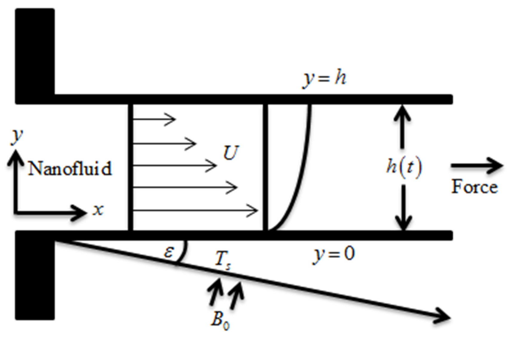
2. Mathematical Modeling

We have assumed the laminar and incompressible thin film flow of second grade fluid containing carbon nanotubes (CNTs) over a linearly extending sheet with Cattaneo–Christov model of heat flux. The stretching sheet is positioned at the starting point of a coordinate system $\left(x,y\right)$ as displayed in Figure 1. The stretching sheet moves along x-direction with a velocity $U_w\left(x,t\right)=\frac{bx}{\left(1-\alpha t\right)}$ where $\alpha$ and $b$ are constants, and temperature is considered as $T_w\left(x,y\right)$. The width of the thin film flow is $h\left(x,y\right)$. Along the extending surface, a variable magnetic field of $B\left(x,t\right)=\frac{B_0}{{\left(1-at\right)}^{\frac{1}{2}}}$ is applied with an allied angle $\epsilon$. The stream function $\xi$ is taken such that $u=\frac{\partial \xi }{\partial y}$ and $v=-\frac{\partial \xi }{\partial x}$.

Figure 1. Gometry of the flow problem.

The Cauchy stress tensor in a second-grade fluid is [43,44]

$$\mathsf{{\rm T}}=\mu {\mathrm{A}}_1+{\alpha }_1{\mathrm{A}}_2+{\alpha }_1{\mathrm{A}}_1^2-p\mathsf{{\rm I}},$$

(1)

$${\mathrm{A}}_1=\left(\mathrm{grad}V\right)+{\left(\mathrm{grad}V\right)}^{\mathsf{{\rm T}}},$$

(2)

$${\mathrm{A}}_2=\frac{d{\mathrm{A}}_1}{dt}+{\mathrm{A}}_1\left(\mathrm{grad}V\right)+{\left(\mathrm{grad}V\right)}^{\mathsf{{\rm T}}}{\mathrm{A}}_1,$$

(3)

where ${\alpha }_1$ and ${\alpha }_2$ are material parameters, $\mu$ is dynamic viscosity, $p$ is the pressure, $\mathsf{{\rm I}}$ is the identity tensor, ${\mathrm{A}}_1$ and ${\mathrm{A}}_2$ are Rivlin–Ericksen tensors defined above, $d/dt$ is the material time derivative, and $V$ is the velocity of the fluid. The Clausius–Duhem inequality is verified and Helmholtz free energy is minimum in equilibrium for the fluid locally at rest when [43,44]

$$\mu \ge 0,{\alpha }_1\ge 0,{\alpha }_1+{\alpha }_2=0.$$

(4)

When ${\alpha }_1+{\alpha }_2=0$, the second grade fluid equation reduces to viscous fluid. Applying the above assumptions, the governing equations can be specified as [46]

$$\frac{\partial u}{\partial x}+\frac{\partial v}{\partial y}=0,$$

(5)

$$v\frac{\partial u}{\partial y}+u\frac{\partial u}{\partial x}+\frac{\partial u}{\partial t}={\upsilon }_{nf}\frac{{\partial }^{2}u}{\partial y^2}+\frac{{\alpha }_1}{{\rho }_{nf}}[\frac{{\partial }^{3}u}{\partial t\partial y^2}+\frac{{\partial }^{2}v}{\partial y^2}\frac{\partial u}{\partial y}+v\frac{{\partial }^{3}u}{\partial y^3}+u\frac{{\partial }^{3}u}{\partial x\partial y^2}+\frac{{\partial }^{2}u}{\partial y^2}\frac{\partial u}{\partial x}]+\frac{{\sigma }_{nf}}{{\rho }_{nf}}{B}^2\left(t\right)u{\cos }^2\epsilon ,$$

(6)

$$\begin{array}{l}{\left(\rho c_p\right)}_{nf}\left(v\frac{\partial T}{\partial y}+u\frac{\partial T}{\partial x}+\frac{\partial T}{\partial t}\right)+{\lambda }_2[\frac{{\partial }^{2}T}{\partial t^2}+\frac{\partial u}{\partial t}\frac{\partial T}{\partial x}+2u\frac{{\partial }^{2}T}{\partial t\partial x}+2v\frac{{\partial }^{2}T}{\partial t\partial y}+\frac{\partial v}{\partial t}\frac{\partial T}{\partial y}\\ +v\frac{\partial T}{\partial y}\frac{\partial v}{\partial y}+u^2\frac{{\partial }^{2}T}{\partial x^2}+v^2\frac{{\partial }^{2}T}{\partial y^2}+u\frac{\partial T}{\partial x}\frac{\partial u}{\partial x}+2uv\frac{{\partial }^{2}T}{\partial x\partial y}+u\frac{\partial T}{\partial y}\frac{\partial v}{\partial x}+v\frac{\partial T}{\partial x}\frac{\partial u}{\partial y}]=\\ \left(k_{nf}+\frac{16}{3}\frac{T_{\infty }^3{\sigma }^{*}}{k^{*}}\right)\frac{{\partial }^{2}T}{\partial y^2}+{\alpha }_1\left[\frac{\partial u}{\partial y}\frac{{\partial }^{2}u}{\partial t\partial y}+u\frac{\partial u}{\partial y}\frac{{\partial }^{2}u}{\partial x\partial y}+v\frac{\partial u}{\partial y}\frac{{\partial }^{2}u}{\partial y^2}\right]+q^{‴},\end{array}$$

(7)

The boundary conditions are defined as:

$$\begin{array}{l}-{\xi }_x=0,{\xi }_y=U_w,T=T_s,\mathrm{at}\hspace{0.17em}y=0,\\ {\xi }_{yy}=0,-{\xi }_x=h_t,T=0,\mathrm{as}\hspace{0.17em}y=h\left(t\right).\end{array}$$

(8)

In the above equations, $u$ and $v$ are velocity components along $x-$ and $y-$ directions respectively, ${\upsilon }_{nf}$ is the kinematic viscosity of the nanofluid, ${\alpha }_1$ is the non- dimensionless second grade fluid parameter, ${\rho }_{nf}$ is the density of the nanofluid, ${\sigma }_{nf}$ is the electrical conductivity of the nanofluid, $c_p$ is the specific heat on the nanofluid, ${\lambda }_2$ is the Cattaneo–Christov parameter, $k_{nf}$ is the thermal conductivity of the nanofluid, ${\sigma }^{*}$ is the Stephan–Boltzmann constant, $k^{*}$ is the mean absorption coefficient, and $q^{‴}$ is the non-uniform heat source/sink term.

$q^{‴}$ is defined as

$$q^{‴}=\frac{k_f{U}_w\left(T_s-T_0\right)}{x{\upsilon }_f}\left(B^{*}\frac{\left(T-T_0\right)}{\left(T_s-T_0\right)}+A^{*}{f}^{\prime }\right).$$

(9)

According to Xue model [47]

$$\begin{array}{l}{\mu }_{nf}=\frac{{\mu }_f}{{\left(1-\varphi \right)}^{5/2}},{\rho }_{nf}=\varphi {\rho }_{CNT}+\left(1-\varphi \right){\rho }_f,{\alpha }_{nf}=\frac{k_{nf}}{{\rho }_{nf}{\left(c_p\right)}_{nf}},{\upsilon }_{nf}=\frac{{\mu }_{nf}}{{\rho }_{nf}},\\ \frac{{\sigma }_{nf}}{{\sigma }_f}=1+\frac{3\sigma \varphi -3\varphi }{\sigma +2-\sigma \varphi +\varphi },\sigma =\frac{{\sigma }_{CNT}}{{\sigma }_f},\frac{k_{nf}}{k_f}=\frac{2\varphi \frac{k_{CNT}}{k_{CNT}-k_f}\ln \left(\frac{k_{CNT}+k_f}{2k_f}\right)+\left(1-\varphi \right)}{2\varphi \frac{k_f}{k_{CNT}-k_f}\ln \left(\frac{k_{CNT}+k_f}{2k_f}\right)+\left(1-\varphi \right)}.\end{array}$$

(10)

The similarity variables are defined as

$$\xi =\beta \sqrt{\frac{b{\nu }_f}{\left(1-at\right)}}xf\left(\eta \right),\theta =\frac{T-T_0}{T_s-T_0},T_s=T_0-\frac{T_r}{{\left(1-at\right)}^{1.5}}\left(\frac{b{x}^2}{2{\nu }_f}\right)\theta \left(\eta \right),\eta =\sqrt{\frac{b}{{\nu }_f\left(1-at\right)}}\frac{y}{\beta }.$$

(11)

Using Equation (11), the continuity equation is obvious, and Equations (6) and (7) yield

$$\begin{array}{l}{f}^{‴}+{\left(1-\varphi \right)}^{2.5}\left(1-\varphi +\varphi \frac{{\rho }_{CNT}}{{\rho }_f}\right)\lambda \left[f{f}^{″}-{f^{\prime }}^2-S\left(f^{\prime }+\frac{1}{2}\eta f^{″}\right)\right]+\alpha {\left(1-\varphi \right)}^{2.5}\\ \left(2f{f}^{‴}+S\left(2f^{‴}+\frac{1}{2}\eta f^{\left(iv\right)}\right)-f{f}^{\left(iv\right)}-{f^{″}}^2\right)-{\left(1-\varphi \right)}^{2.5}\frac{{\sigma }_{nf}}{{\sigma }_f}M{f}^{\prime }{\cos }^2\epsilon =0,\end{array}$$

(12)

$$\begin{array}{l}\frac{\left[\frac{k_{nf}}{k_f}+\frac{4}{3}Rd\right]}{\mathrm{Pr}\left[1-\varphi +\varphi \frac{{\left(\rho c_p\right)}_{CNT}}{{\left(\rho c_p\right)}_f}\right]}{\theta }^{″}+\frac{1}{\mathrm{Pr}\left[1-\varphi +\varphi \frac{{\left(\rho c_p\right)}_{CNT}}{{\left(\rho c_p\right)}_f}\right]}\left(A^{*}{f}^{\prime }+B^{*}\theta \right)-\lambda \left[2f^{\prime }\theta -f{\theta }^{\prime }+\frac{S}{2}\left(3\theta +\eta {\theta }^{\prime }\right)\right]\\ +\alpha Ec\left[\begin{array}{l}\frac{S}{2}\left(3{f^{″}}^2+\eta f^{″}{f}^{‴}\right)\\ +f^{\prime }{f^{″}}^2-f{f}^{″}{f}^{‴}\end{array}\right]+\gamma \left[\begin{array}{l}-\frac{15}{2}{S}^2\theta -\frac{7}{2}{S}^2\eta {\theta }^{\prime }-\frac{1}{4}{S}^2{\eta }^2{\theta }^{″}-8S{f}^{\prime }\theta -\eta S{f}^{″}\theta +\frac{9}{2}Sf{\theta }^{\prime }\\ -\frac{3}{2}\eta S{f}^{\prime }{\theta }^{\prime }+\eta Sf{\theta }^{″}-4{f^{\prime }}^2\theta -{f^{\prime }}^2{\theta }^{″}+2f{f}^{″}\theta +3f{f}^{\prime }{\theta }^{\prime }\end{array}\right]=0,\end{array}$$

(13)

with

$$\begin{array}{l}f=0,f^{\prime }=\theta =1\mathrm{at}\hspace{0.17em}\eta =0,\\ f=\frac{S}{2},f^{″}={\theta }^{\prime }=0,\mathrm{at}\hspace{0.17em}\eta =1.\end{array}$$

(14)

In the above equations, $\varphi$ signifies nanoparticles volume fraction, $\lambda$ represents the film thickness, $S$ indicates the unsteadiness parameter, $\alpha$ indicates the dimensionless second grade fluid parameter, $M$ is the magnetic parameter, $\mathrm{Pr}$ is the Prandtl number, $Rd$ represents the thermal radiation parameter, $A^{*},B^{*}$ are the heat source/sink parameters, $Ec$ is the Eckert number, and $\gamma$ is the thermal relaxation parameter.

The dimensionless parameters are defined as

$$\mathrm{Pr}=\frac{{\nu }_f}{{\alpha }_f},S=\frac{a}{b},Rd=\frac{4{\sigma }^{*}{T}_0^3}{k^{*}{k}_f},M=\frac{{\sigma }_f{B}_0^2}{b{\rho }_f},\gamma =\frac{{\lambda }_{2}b}{\left(1-at\right)},\lambda ={\beta }^2,Ec=\frac{U_w^2}{c_p(T_s-T_{\infty })},\alpha =\frac{b{\alpha }_1}{{\mu }_f\left(1-at\right)}.$$

(15)

3. Physical Quantities

3.1. Surface Drag Force

The skin friction coefficient is defined as

$$C_f=\frac{{\tau }_w}{{\rho }_f{U}_w^2},$$

(16)

where

$${\tau }_w={\left[{\mu }_{nf}\frac{\partial u}{\partial y}+{\alpha }_1\left(\frac{{\partial }^{2}u}{\partial t\partial y}+u\frac{{\partial }^{2}u}{\partial x\partial y}+2\frac{\partial u}{\partial y}\frac{\partial u}{\partial x}+v\frac{{\partial }^{2}u}{\partial y^2}\right)\right]|}_{y=0}.$$

(17)

Using Equation (11), Equations (16) and (17) are reduced as

$$C_f{\mathrm{Re}}_x^{\frac{1}{2}}={\left[\frac{1}{\beta {\left(1-\varphi \right)}^{2.5}}{f}^{″}\left(\eta \right)+\alpha \left(3f^{″}\left(\eta \right)f^{\prime }\left(\eta \right)-f^{‴}\left(\eta \right)f\left(\eta \right)+\frac{S}{2}\left(\eta f^{‴}\left(\eta \right)+3f^{″}\left(\eta \right)\right)\right)\right]|}_{\eta =0}.$$

(18)

3.2. Heat Transfer Rate

The heat transfer rate is defined as

$$N{u}_x=\frac{x{q}_w}{k_{nf}\left(T_s-T_0\right)},$$

(19)

$$q_w={-k_{nf}\left(\frac{\partial T}{\partial y}\right)|}_{y=0}$$

(20)

Using Equation (11), the dimensionless form of Equations (19) and (20) are reduced as

$$Nu{\mathrm{Re}}_x^{-\frac{1}{2}}={-\frac{1}{\beta }\left(\frac{k_{nf}}{k_f}+\frac{4}{3}Rd\right){\theta }^{\prime }\left(\eta \right)|}_{\eta =0}.$$

(21)

where ${\mathrm{Re}}_x=\frac{b{x}^2}{{\upsilon }_f\left(1-at\right)}$.

4. Entropy Generation

Entropy generation for the above mentioned suppositions is

$$\begin{array}{l}{E}_{gen}=\frac{k_f}{T_0^2}\left[\frac{k_{nf}}{k_f}+\frac{16}{3}\frac{T_{\infty }^3{\sigma }^{*}}{k^{*}{k}_f}\right]{\left(\frac{\partial T}{\partial y}\right)}^2+\frac{{\mu }_{nf}}{T_0}{\left(\frac{\partial u}{\partial y}\right)}^2+\\ \frac{{\alpha }_1}{T_0}\left[\frac{{\partial }^{2}u}{\partial t\partial y}\frac{\partial u}{\partial y}+u\frac{{\partial }^{2}u}{\partial x\partial y}\frac{\partial u}{\partial y}+v\frac{{\partial }^{2}u}{\partial y^2}\frac{\partial u}{\partial y}\right]+\frac{{\sigma }_{nf}}{T_0}{B}^2\left(t\right)u^2{\cos }^2\epsilon .\end{array}$$

(22)

Using Equation (11), the dimensionless form of Equation (20) is

$$\begin{array}{l}{N}_G=\left[\frac{k_{nf}}{k_f}+\frac{4}{3}Rd\right]\mathrm{Re}{{\theta }^{\prime }}^2+\frac{1}{{\left(1-\varphi \right)}^{2.5}}\frac{Br\mathrm{Re}}{{\alpha }_2}{f^{″}}^2+\\ \frac{\alpha Br\mathrm{Re}}{{\alpha }_2}\left[\frac{S}{2}\left(3{f^{″}}^2+\eta f^{″}{f}^{‴}\right)+f^{\prime }{f^{″}}^2-f{f}^{″}{f}^{‴}\right]+\frac{BrM}{{\alpha }_2}\frac{{\sigma }_{nf}}{{\sigma }_f}{\cos }^2\epsilon {f^{\prime }}^2.\end{array}$$

(23)

where

$${\alpha }_2=\frac{\Delta T}{T_w},Br=\frac{{\mu }_f{U}_w^2}{\Delta T{k}_f},\mathrm{Re}=\frac{U_{w}x}{{\nu }_f}.$$

(24)

where ${\mathsf{{\rm N}}}_G,{\alpha }_2$ and $Br,\mathrm{Re}$ indicate the rate of entropy optimization rate, gradient of temperature, Brinkman number, and Reynold’s number, respectively.

5. HAM Solution

To solve Equations (12) and (13) with (14) by using HAM, it is assumed that $f=V$ and $\theta =H$. Initial guesses and linear operators are

$$V_0\left(\eta \right)=\frac{1}{4}\left(4\eta -6{\eta }^2+3S{\eta }^2+2{\eta }^3-S{\eta }^3\right),H_0\left(\eta \right)=1+2\eta -{\eta }^2,$$

(25)

$$L_V=V^{‴},L_H=H^{″},$$

(26)

$$L_V\left[{\mathsf{\Omega }}_1+{\mathsf{\Omega }}_2\eta +{\mathsf{\Omega }}_3{\eta }^2+{\mathsf{\Omega }}_4{\eta }^3\right]=0,L_H\left[{\mathsf{\Omega }}_5+{\mathsf{\Omega }}_6\eta +{\mathsf{\Omega }}_7{\eta }^2\right]=0,$$

(27)

where ${\mathsf{\Omega }}_i\left(i=1,2,3,\dots ,7\right)$ are arbitrary constants.

$0^{th}-$ order problems

Assume that $W\in \left[0,1\right]$ be the rooted factor and ${\hslash }_V$ and ${\hslash }_H$ are the non-zero supporting factors, then

$$\left(1-W\right)L_V\left[V\left(\eta ;W\right)-V_0\left(\eta \right)\right]=W{\hslash }_V{\aleph }_V\left[V\left(\eta ;W\right)\right],$$

(28)

$$\left(1-W\right)L_H\left[H\left(\eta ;W\right)-H_0\left(\eta \right)\right]=W{\hslash }_H{\aleph }_H\left[H\left(\eta ;W\right)\right],$$

(29)

$$V\left(0;W\right)=0,V^{\prime }\left(0;W\right)=1,H\left(0;W\right)=1,V\left(1;W\right)=\frac{S}{2},V^{″}\left(1;W\right)=0,H^{\prime }\left(1;W\right)=0.$$

(30)

$$\begin{array}{l}{\aleph }_V\left[V\left(\eta ;W\right)\right]=\frac{{\partial }^{3}V\left(\eta ;W\right)}{\partial {\eta }^3}+{\left(1-\varphi \right)}^{2.5}\left(1-\varphi +\varphi \frac{{\rho }_{CNT}}{{\rho }_f}\right)\lambda [V\left(\eta ;p\right)\frac{{\partial }^{2}V\left(\eta ;W\right)}{\partial {\eta }^2}-{\left(\frac{\partial V\left(\eta ;W\right)}{\partial \eta }\right)}^2\\ -S\left(\frac{\partial V\left(\eta ;W\right)}{\partial \eta }+\frac{1}{2}\eta \frac{{\partial }^{2}V\left(\eta ;W\right)}{\partial {\eta }^2}\right)]+\alpha {\left(1-\varphi \right)}^{2.5}[2V\left(\eta ;W\right)\frac{{\partial }^{3}V\left(\eta ;W\right)}{\partial {\eta }^3}+S(2\frac{{\partial }^{3}V\left(\eta ;W\right)}{\partial {\eta }^3}+\\ \frac{1}{2}\eta \frac{{\partial }^{4}V\left(\eta ;W\right)}{\partial {\eta }^4})-V\left(\eta ;W\right)\frac{{\partial }^{4}V\left(\eta ;W\right)}{\partial {\eta }^4}-{\left(\frac{{\partial }^{2}V\left(\eta ;W\right)}{\partial {\eta }^2}\right)}^2]-{\left(1-\varphi \right)}^{2.5}\frac{{\sigma }_{nf}}{{\sigma }_f}M\frac{\partial V\left(\eta ;W\right)}{\partial \eta }{\cos }^2\epsilon ,\end{array}$$

(31)

$$\begin{array}{l}{\aleph }_H\left[H\left(\eta ;W\right);V\left(\eta ;W\right)\right]=\frac{\left[\frac{k_{nf}}{k_f}+\frac{4}{3}Rd\right]}{\mathrm{Pr}\left[1-\varphi +\varphi \frac{{\left(\rho c_p\right)}_{CNT}}{{\left(\rho c_p\right)}_f}\right]}\frac{{\partial }^{2}H\left(\eta ;W\right)}{\partial {\eta }^2}+\frac{1}{\mathrm{Pr}\left[1-\varphi +\varphi \frac{{\left(\rho c_p\right)}_{CNT}}{{\left(\rho c_p\right)}_f}\right]}\\ \left(\begin{array}{l}{A}^{*}\frac{\partial V\left(\eta ;W\right)}{\partial \eta }\\ +B^{*}H\left(\eta ;W\right)\end{array}\right)-\lambda \left[2\frac{\partial V\left(\eta ;W\right)}{\partial \eta }H\left(\eta ;W\right)-V\left(\eta ;W\right)\frac{\partial H\left(\eta ;W\right)}{\partial \eta }+\frac{S}{2}\left(3H\left(\eta ;W\right)+\eta \frac{\partial H\left(\eta ;W\right)}{\partial \eta }\right)\right]\\ +\gamma [-\frac{15}{2}{S}^{2}H\left(\eta ;W\right)-\frac{7}{2}{S}^2\eta \frac{\partial H\left(\eta ;W\right)}{\partial \eta }-8SH\left(\eta ;W\right)\frac{\partial V\left(\eta ;W\right)}{\partial \eta }-\eta SH\left(\eta ;W\right)\frac{{\partial }^{2}V\left(\eta ;W\right)}{\partial {\eta }^2}\\ -\frac{3}{2}\eta S\frac{\partial V\left(\eta ;W\right)}{\partial \eta }\frac{\partial H\left(\eta ;W\right)}{\partial \eta }-\frac{1}{4}{S}^2{\eta }^2\frac{{\partial }^{2}H\left(\eta ;W\right)}{\partial {\eta }^2}+\frac{9}{2}SV\left(\eta ;W\right)\frac{\partial H\left(\eta ;W\right)}{\partial \eta }+\\ \eta SV\left(\eta ;W\right)\frac{{\partial }^{2}H\left(\eta ;W\right)}{\partial {\eta }^2}-4H\left(\eta ;W\right){\left(\frac{\partial V\left(\eta ;W\right)}{\partial \eta }\right)}^2-{\left(\frac{\partial V\left(\eta ;W\right)}{\partial \eta }\right)}^2\frac{{\partial }^{2}H\left(\eta ;W\right)}{\partial {\eta }^2}\\ +3V\left(\eta ;W\right)\frac{\partial V\left(\eta ;W\right)}{\partial \eta }\frac{\partial H\left(\eta ;W\right)}{\partial \eta }+2V\left(\eta ;W\right)H\left(\eta ;W\right)\frac{{\partial }^{2}V\left(\eta ;W\right)}{\partial {\eta }^2}]+\\ \alpha Ec[\frac{S}{2}(3{\left(\frac{{\partial }^{2}V\left(\eta ;W\right)}{\partial {\eta }^2}\right)}^2+\eta \frac{{\partial }^{2}V\left(\eta ;W\right)}{\partial {\eta }^2}\frac{{\partial }^{3}V\left(\eta ;W\right)}{\partial {\eta }^3})\\ +\frac{\partial V\left(\eta ;W\right)}{\partial \eta }{\left(\frac{{\partial }^{2}V\left(\eta ;W\right)}{\partial {\eta }^2}\right)}^2-V\left(\eta ;W\right)\frac{{\partial }^{2}V\left(\eta ;W\right)}{\partial {\eta }^2}\frac{{\partial }^{3}V\left(\eta ;W\right)}{\partial {\eta }^3}],\end{array}$$

(32)

$k^{th}-$ order problems

$k^{th}-$ order problems are

$$L_V\left[V_k\left(\eta \right)-{\chi }_k{V}_{k-1}\left(\eta \right)\right]={\hslash }_k{\Re }_k^V\left(\eta \right),$$

(33)

$$L_H\left[H_k\left(\eta \right)-{\chi }_k{H}_{k-1}\left(\eta \right)\right]={\hslash }_H{\Re }_k^H\left(\eta \right),$$

(34)

$$V_k\left(0\right)=V_k^{\prime }\left(0\right)=V_k\left(1\right)=V_k^{″}\left(1\right)=H_k\left(0\right)=H_k^{\prime }\left(1\right)=0.$$

(35)

$$\begin{array}{l}{\Re }_k^V\left(\eta \right)=V_{k-1}^{‴}+{\left(1-\varphi \right)}^{2.5}\left(1-\varphi +\varphi \frac{{\rho }_{CNT}}{{\rho }_f}\right)\lambda \left[\begin{array}{l}{\displaystyle \sum _{j=0}^{k-1}\left(V_{k-1-j}{V}_{j-1}^{″}\right)}-{\left(V_{k-1}^{\prime }\right)}^2\\ -S\left(V_{k-1}^{\prime }+\frac{1}{2}\eta V_{k-1}^{″}\right)\end{array}\right]+\\ \alpha {\left(1-\varphi \right)}^{2.5}\left[\begin{array}{l}2{\displaystyle \sum _{j=0}^{k-1}\left(V_{k-1-j}{V}_{j-1}^{‴}\right)}+S\left(2V_{k-1}^{‴}+\frac{1}{2}\eta V_{k-1}^{\left(iv\right)}\right)\\ -{\displaystyle \sum _{j=0}^{k-1}\left(V_{k-1-j}{V}_{k-1}^{\left(iv\right)}\right)-}{\left(V_{k-1}^{″}\right)}^2\end{array}\right]-{\left(1-\varphi \right)}^{2.5}\frac{{\sigma }_{nf}}{{\sigma }_f}M{V}_{k-1}^{\prime }{\cos }^2\epsilon ,\end{array}$$

(36)

$$\begin{array}{l}{\Re }_k^H\left(\eta \right)=\frac{\left[\frac{k_{nf}}{k_f}+\frac{4}{3}Rd\right]}{\mathrm{Pr}\left[1-\varphi +\varphi \frac{{\left(\rho c_p\right)}_{CNT}}{{\left(\rho c_p\right)}_f}\right]}{H}_{k-1}^{″}+\frac{1}{\mathrm{Pr}\left[1-\varphi +\varphi \frac{{\left(\rho c_p\right)}_{CNT}}{{\left(\rho c_p\right)}_f}\right]}\left(A^{*}{V}_{k-1}^{\prime }+B^{*}{H}_{k-1}\right)\\ -\lambda \left[2{\displaystyle \sum _{j=0}^{k-1}\left(V_{k-1-j}^{\prime }{H}_{k-1}\right)}-{\displaystyle \sum _{j=0}^{k-1}\left(V_{k-1-j}{H}_{k-1}^{\prime }\right)}+\frac{S}{2}\left(3H_{k-1}+\eta H_{k-1}^{\prime }\right)\right]+\gamma [-\frac{15}{2}{S}^2{H}_{k-1}-\frac{7}{2}{S}^2\eta H_{k-1}^{\prime }\\ -8S{\displaystyle \sum _{j=0}^{k-1}\left(V_{k-1-j}^{\prime }{H}_{k-1}\right)}-\eta S{\displaystyle \sum _{j=0}^{k-1}\left(V_{k-1-j}^{″}{H}_{k-1}^{\prime }\right)}-\frac{3}{2}\eta S{\displaystyle \sum _{j=0}^{k-1}\left(V_{k-1-j}^{\prime }{H}_{k-1}^{\prime }\right)}+\frac{9}{2}S{\displaystyle \sum _{j-0}^{k-1}\left(V_{k-1-j}{H}_{k-1}^{\prime }\right)}+\\ \eta S{\displaystyle \sum _{j=0}^{k-1}\left(V_{k-1-j}{H}_{k-1}^{″}\right)}-4{\displaystyle \sum _{j=0}^{k-1}\left({V^{\prime }}_{k-1-j}^2{H}_{k-1}^{\prime }\right)}+3{\displaystyle \sum _{j=0}^{k-1}\left(V_{k-1-j}{V}_{k-1}^{\prime }{H}_k^{\prime }\right)}-{\displaystyle \sum _{j=0}^{k-1}\left({V^{\prime }}_{k-1-j}^2{H}_{k-1}^{″}\right)}+-\frac{1}{4}{S}^2{\eta }^2{H^{″}}_{k-1}^2\\ 2{\displaystyle \sum _{j=0}^{k-1}\left(V_{k-1-j}{V}_{k-1}^{″}{H}_k\right)}]+\alpha Ec\left[\frac{S}{2}\left(3{V^{″}}_{k-1}^2+\eta {\displaystyle \sum _{j=0}^{k-1}\left(V_{k-1-j}^{″}{V}_{k-1}^{‴}\right)}\right)+{\displaystyle \sum _{j=0}^{k-1}\left(V_{k-1-j}^{\prime }{V^{″}}_{k-1}^2\right)}-{\displaystyle \sum _{j=0}^{k-1}\left(V_{k-1-j}{V}_{k-1}^{″}{V}_k^{‴}\right)}\right].\end{array}$$

(37)

When $W=0$ and $W=1$, we can write

$$V\left(\eta ;0\right)=V_0\left(\eta \right),V\left(\eta ;1\right)=V\left(\eta \right),$$

(38)

$$H\left(\eta ;0\right)=H_0\left(\eta \right),H\left(\eta ;1\right)=H\left(\eta \right),$$

(39)

By Taylor’s expansion

$$V\left(\eta ;W\right)=V_0\left(\eta \right)+{\displaystyle \sum _{k=1}^{\infty }{V}_k\left(\eta \right)}{W}^k,{V_k\left(\eta ;W\right)=\frac{1}{k!}\frac{{\partial }^{k}V\left(\eta ;W\right)}{\partial W^k}|}_{w=0},$$

(40)

$$H\left(\eta ;W\right)=H_0\left(\eta \right)+{\displaystyle \sum _{k=1}^{\infty }{H}_k\left(\eta \right)}{W}^k,{H_k\left(\eta ;W\right)=\frac{1}{k!}\frac{{\partial }^{k}H\left(\eta ;W\right)}{\partial W^k}|}_{w=0}.$$

(41)

The series (38) and (39) converge at $W=1$, then

$$V\left(\eta \right)=V_0\left(\eta \right)+{\displaystyle \sum _{k=1}^{\infty }{V}_k\left(\eta \right)},$$

(42)

$$H\left(\eta \right)=H_0\left(\eta \right)+{\displaystyle \sum _{k=1}^{\infty }{H}_k\left(\eta \right)},$$

(43)

where

$${\chi }_k=\{\begin{array}{l}0,k\le 1,\\ 1,k>1.\end{array}$$

(44)

Convergence of HAM

Auxiliary factors ${\hslash }_f$ and ${\hslash }_{\theta }$ play an imperative character in convergence regions for velocity and temperature functions. Here, in Figure 2 at 25th order of approximations, the $\hslash -$ curves are schemed. The ranges for velocity and temperature profiles are $-4.0\le {\hslash }_f\le 3.0$ and $-0.04\le {\hslash }_{\theta }\le 0.04$ respectively. Table 2 show numerically the convergent of homotopy analysis method.

Figure 2. Combine $\hslash -$ curve for velocity and temperature distribution profiles when $\mathrm{Pr}=1.0,$ $S=0.2,Rd=0.3,$ $M=1.5,$ $\gamma =0.1,$ $\lambda =0.5$ and $\alpha =0.2$.

Table 2. Convergence table for $f^{\prime }\left(\eta \right)$ and $\theta \left(\eta \right)$ when $\mathrm{Pr}=1.0,$ $S=0.2,Rd=0.3,$ $M=1.5,$ $\gamma =0.1,$ $\lambda =0.5$ and $\alpha =0.2$.

$\mathit{\eta }$	${\mathit{f}}^{\prime }\left(\mathit{\eta }\right)$	$\mathit{\theta }\left(\mathit{\eta }\right)$
5	0.856220	0.75423
10	0.856222	0.75443
15	0.860002	0.75458
20	0.860001	0.75467
25	0.860001	0.75467

6. Results and Discussion

This segment covers the discussion about physical effect of the embedded factors $(0.0\le \varphi \le 0.2)$, $(1.0\le S\le 4.0)$, $(0.0\le M\le 3.0)$, $(0.1\le \lambda \le 3.0)$, $(0.01\le \alpha \le 5.0)$, $(0.1\le A^{*}\le 0.5)$, $(0.1\le B^{*}\le 0.5)$, $(2.0\le Rd\le 4.0)$, $(0.2\le \gamma \le 0.6)$, $(2.0\le Br\le 4.0)$ and $(2.0\le \mathrm{Re}\le 3.0)$ on $f^{\prime }\left(\eta \right)$, $\theta \left(\eta \right)$ and $Ns\left(\eta \right)$ profiles of the thin film flow covering SWCNTs and MWCNTs.

Figure 3 is designed to visualize the accuracy of the model provided by contrasting it with Sandeep [46] and Xu et al. [48], which addressed the nanofluids flow through a thin film under the magnetic impact. Thus, to compare our work, the special effects of all fixed factors are neglected. Great coordination is proven among the established comparison. It should be noted that the red colour represents the increasing values of unsteadiness parameter $S$, black colour represents ref. [46], yellow colour represents ref. [48], and blue colour represents the present values.

Figure 3. Comparison of $-\theta \left(0\right)$ for different estimations of $S$ when $M=Rd=\gamma =\alpha =\lambda =A^{*}=B^{*}=0,\mathrm{Pr}=0.8.$

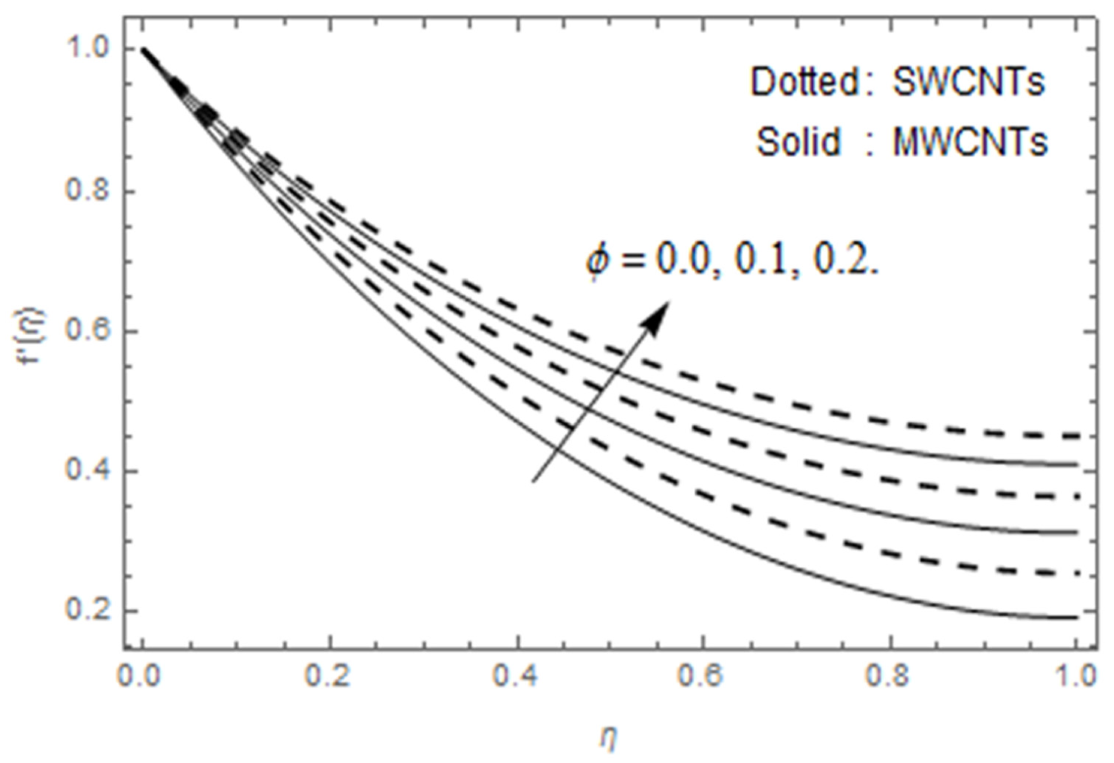
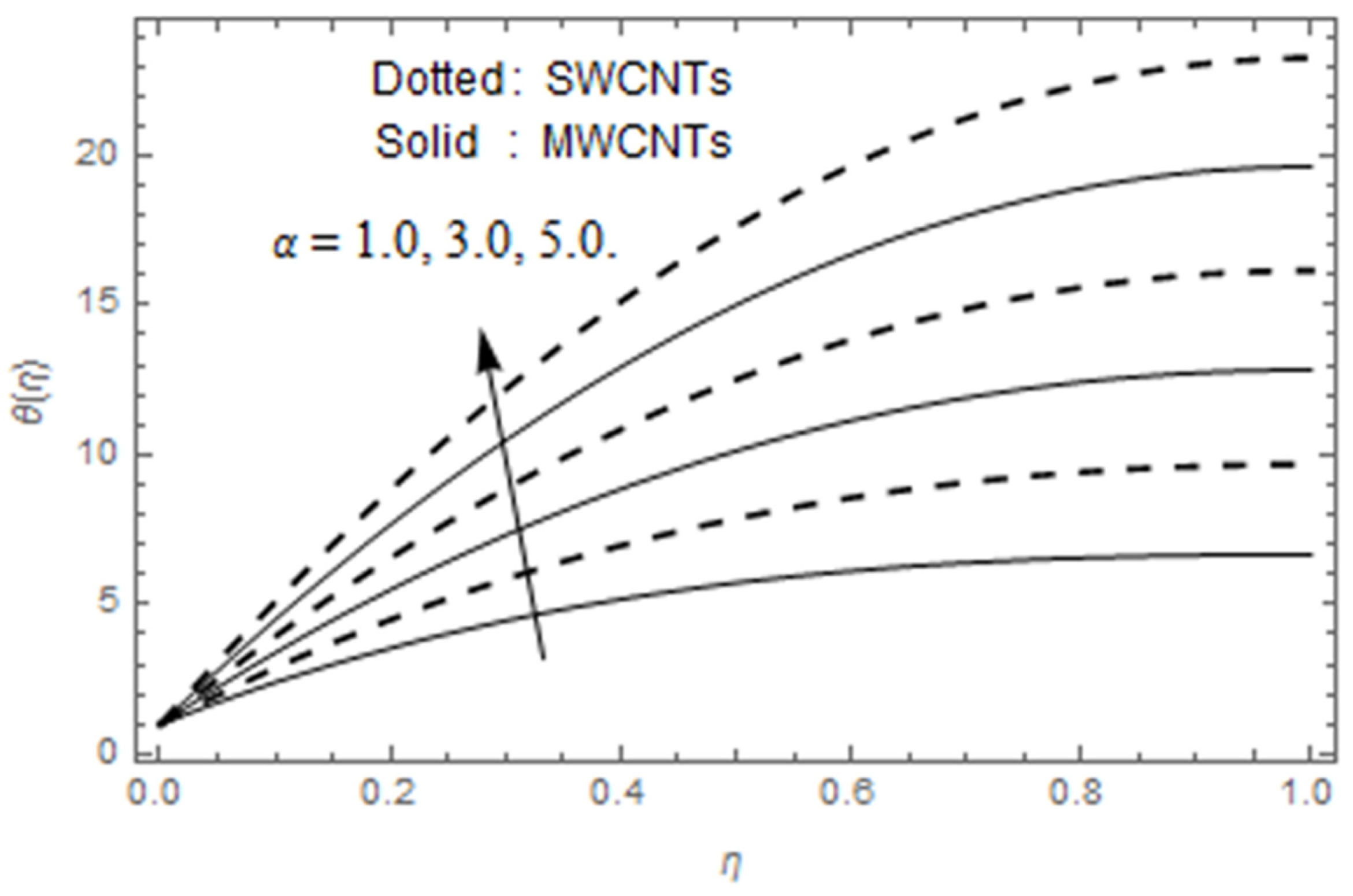
6.1. Velocity and Temperature Functions

The consequences of nanoparticles volume fraction $\varphi$ on velocity $f^{\prime }\left(\eta \right)$ and temperature $\theta \left(\eta \right)$ of the thin film second grade fluid flow containing SWNCTs and MWCNTs are shown in Figure 4 and Figure 5. Both velocity $f^{\prime }\left(\eta \right)$ and temperature $\theta \left(\eta \right)$ profiles heighten with greater values of volume fraction of nanoparticles. The relationship between nanoparticles volume fraction and convective flow is directly proportional. Therefore, the higher estimations of nanoparticles volume fraction $\varphi$ increase fluid velocity $f^{\prime }\left(\eta \right)$ and temperature $\theta \left(\eta \right)$ for both cases of CNTs. The deviation in velocity function $f^{\prime }\left(\eta \right)$ against magnetic parameter $M$ is displayed in Figure 6. Physically, the increasing magnetic field boosts up the Lorentz forces which increases the resistive force to fluid motion and consequently $f^{\prime }\left(\eta \right)$ reduces. Figure 7 and Figure 8 exhibit the variations in $f^{\prime }\left(\eta \right)$ and $\theta \left(\eta \right)$ of the fluid flow via $\lambda$. The higher values of film thickness reduce both profiles of the flow. Increasing liquid film thickness parameter $\lambda$ augmented the viscous forces, in due course $f^{\prime }\left(\eta \right)$ reduces. This complies with the general physical nature of the film thickness parameter. Expanding the film thickness stops to permit the extra liquid. The impact of liquid film thickness parameter $\lambda$ on $\theta \left(\eta \right)$ is shown in Figure 8. A similar impact is observed for the temperature profile. The variations in velocity $f^{\prime }\left(\eta \right)$ and temperature $\theta \left(\eta \right)$ fields via dimensionless second grade fluid par $\alpha$ are shown in Figure 9 and Figure 10. It is perceived that higher estimations of dimensionless second grade fluid par $\alpha$ escalate $f^{\prime }\left(\eta \right)$ and $\theta \left(\eta \right)$ of the fluid flow. Infect there is inverse relation between the viscosity of fluid and $\alpha$. Therefore, the greater values of $\alpha$ moderate the viscosity of the fluid, and accordingly the fluid velocity upsurges. Alike impact is also perceived in temperature profile. The variations in $f^{\prime }\left(\eta \right)$ and $\theta \left(\eta \right)$ via unsteadiness parameter $S$ are displayed in Figure 11 and Figure 12. Both $f^{\prime }\left(\eta \right)$ and $\theta \left(\eta \right)$ reduce with higher estimations of unsteadiness parameter $S$. Physically, due to the greater unsteadiness parameter, the buoyancy effect actions on the flow and declines it. Thus, the momentum and thickness of the thermal boundary layer diminish. The deviation in temperature field $\theta \left(\eta \right)$ via heat source/sink parameters $A^{*}$ and $B^{*}$ is displayed in Figure 13 and Figure 14. Actually, heat source/sink parameters $A^{*}$ and $B^{*}$ act like a heat creator. The greater heat source/sink, the greater heat will produce to the fluid flow. Therefore, temperature profile heightens via $A^{*}$ and $B^{*}$. The variation in $\theta \left(\eta \right)$ via thermal radiation parameter $Rd$ is displayed in Figure 15. $\theta \left(\eta \right)$ increases with the heightens in thermal radiation parameter $Rd$. This effect is because of the datum that the higher estimations of $Rd$ deescalates the mean absorption coefficient and escalates the divergence of radiative heat flux. Therefore, the thermal profile escalates with the rise in $Rd$. The influence of thermal relaxation parameter $\gamma$ on $\theta \left(\eta \right)$ of the fluid flow is publicized in Figure 16. It is depicted that higher estimations of thermal relaxation parameter $\gamma$ reduces $\theta \left(\eta \right)$. From here, it is concluded that the particles require much additional time for transferring of heat to its neighborhood particles and so the heat of the fluid reduces. Therefore, the higher estimations of $\gamma$ reduce $\theta \left(\eta \right)$.

Figure 4. Variation in $f^{\prime }\left(\eta \right)$ via $\varphi$.

Figure 5. Variation in $\theta \left(\eta \right)$ via $\varphi$.

Figure 6. Variation in $f^{\prime }\left(\eta \right)$ via $M$.

Figure 7. Variation in $f^{\prime }\left(\eta \right)$ via $\lambda$.

Figure 8. Variation in $\theta \left(\eta \right)$ via $\lambda$.

Figure 9. Variation in $f^{\prime }\left(\eta \right)$ via $\alpha$.

Figure 10. Variation in $\theta \left(\eta \right)$ via $\alpha$.

Figure 11. Variation in $f^{\prime }\left(\eta \right)$ via $S$.

Figure 12. Variation in $\theta \left(\eta \right)$ via $S$.

Figure 13. Variation in $\theta \left(\eta \right)$ via $A^{*}$.

Figure 14. Variation in $\theta \left(\eta \right)$ via $B^{*}$.

Figure 15. Variation in $\theta \left(\eta \right)$ via $Rd$.

Figure 16. Variation in $\theta \left(\eta \right)$ via $\gamma$.

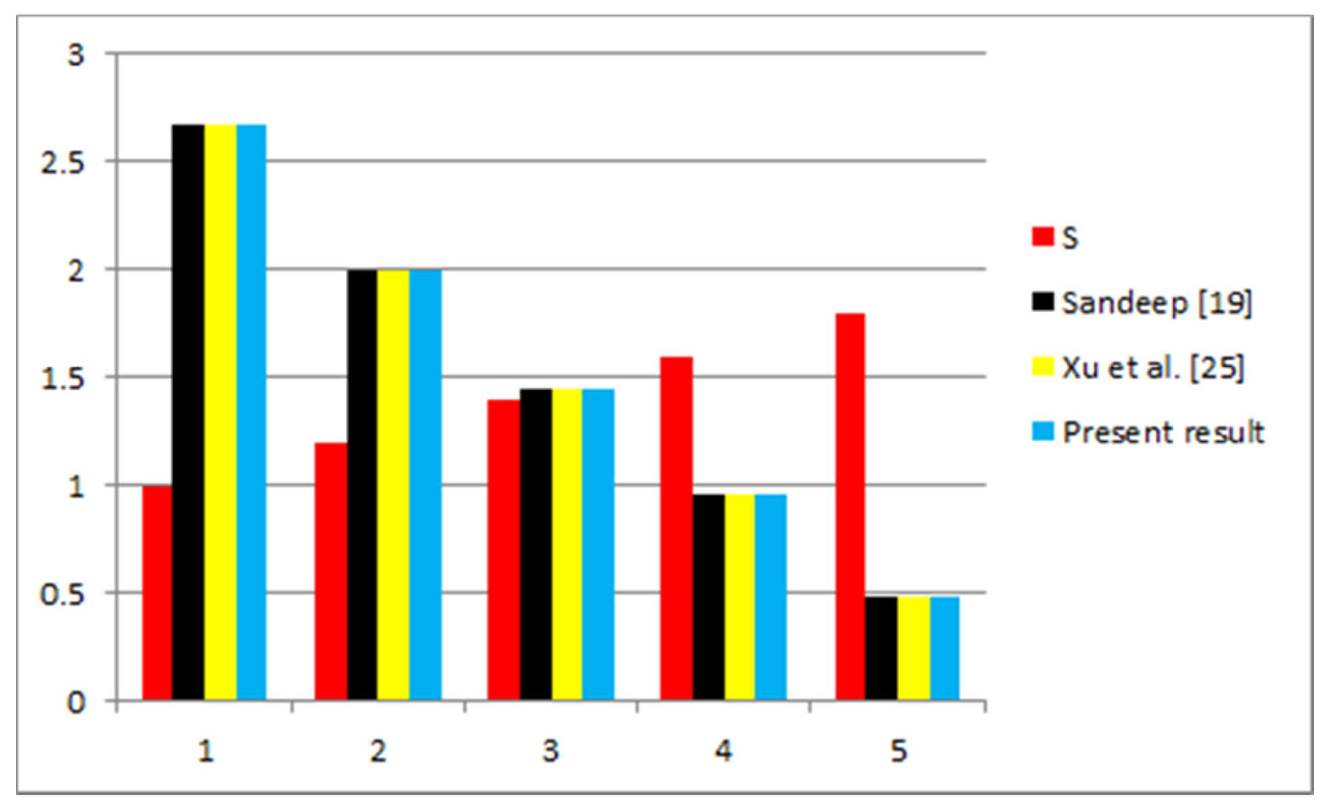
6.2. Skin Friction Coefficient

The engineers take interest to calculate some physical quantities in the flow/circulation of the fluid in some parts of the machinery, like the friction between the extending surface and the nanofluid and thermal transmission rate between the fluids and some solid parts of the mechanical system in the machinery. The friction between the nanofluid and extending sheet also affect the temperature of the nanofluid. This friction between the nanofluid and extending sheet is known as skin friction. Figure 17 is displayed to investigate the surface drag force in a thin film flow containing both SWCNTs and MWCNTs against the dimensionless parameters like nanoparticles volume fraction, unsteadiness, film thickness, magnetic, and second grade fluid. The surface drag force $C_f$ of the thin film flow containing both SWCNTs and MWCNTs heightens against nanoparticles volume fraction, unsteadiness parameter, film thickness, magnetic field parameter, and second grade fluid parameter. It is also depicted that the impact of dimensionless parameters on SWCNTs is dominant compared to MWCNTs. It should be noted that all the three colours (i.e., black, blue, and red) represent the variation in skin friction coefficient due to dimensionless parameters.

Figure 17. Against $\varphi ,S,\lambda ,M$ and $\alpha$.

6.3. Heat Transfer Rate

The engineers also take interest to calculate the rate of heat exchange between the flowing fluids and the solid parts of the surface in contact with fluids. This rate is called Nusselt number which is the ratio between convective thermal transmission and conductive thermal transmission at the specific point in the flow. Figure 18 is displayed to investigate the variation in thermal transfer rate of the thin film flow containing both SWCNTs and MWCNTs via dimensionless parameters. The thermal transmission rate of the thin film flow containing SWCNTs and MWCNTs heightens with the higher estimations of nanoparticles volume fraction, film thickness, and unsteadiness parameter while declines with the higher estimations of heat source and sink. It should be noted that all the three colours (i.e., black, blue, and red) represent the variation in local Nusselt number due to dimensionless parameters.

Figure 18. Against $\varphi ,S,\lambda ,A^{*}$ and $B^{*}$ with $\gamma =0.1,Rd=1.0,\alpha =0.1$ and $\mathrm{Pr}=6.2$.

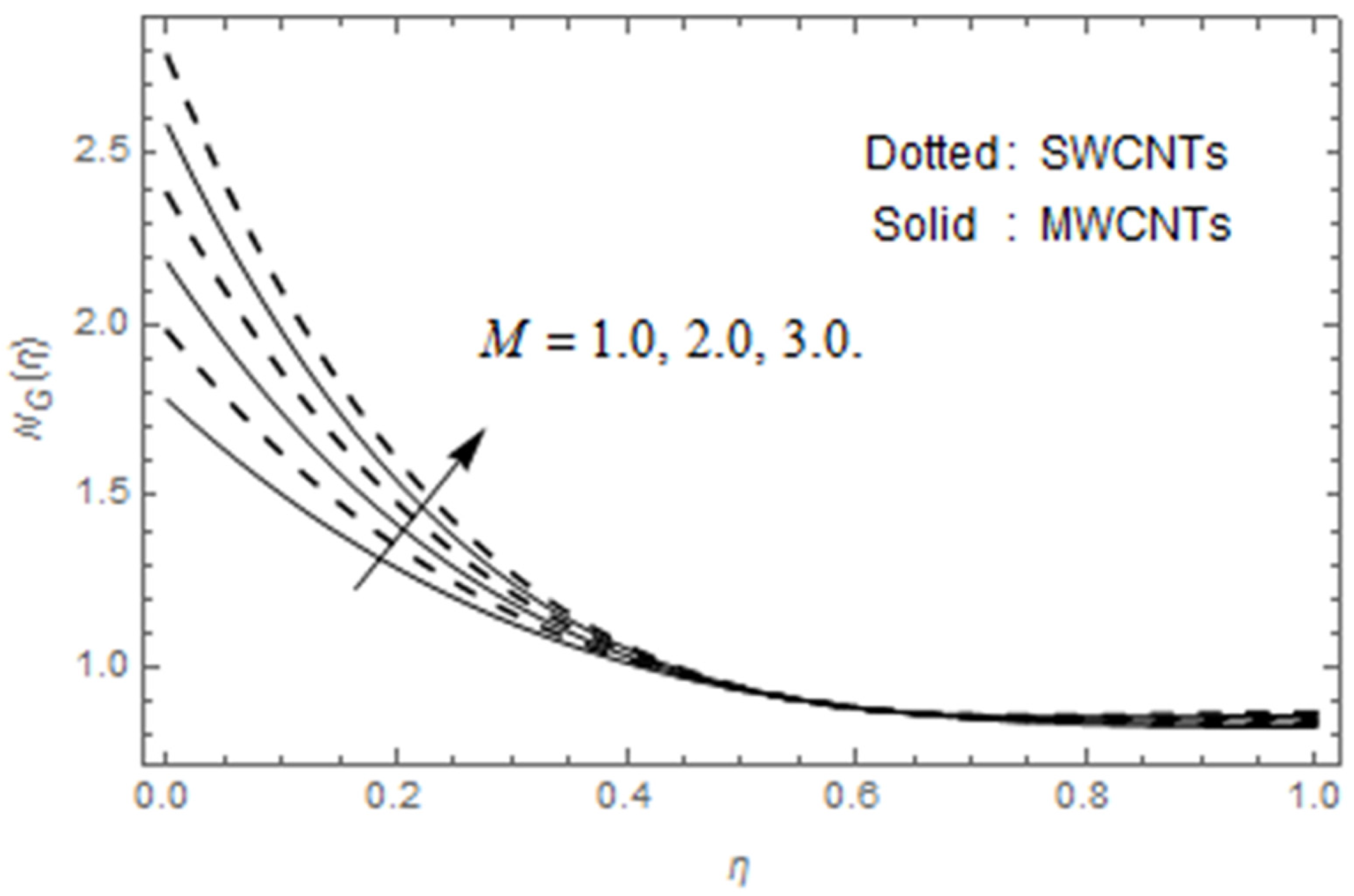
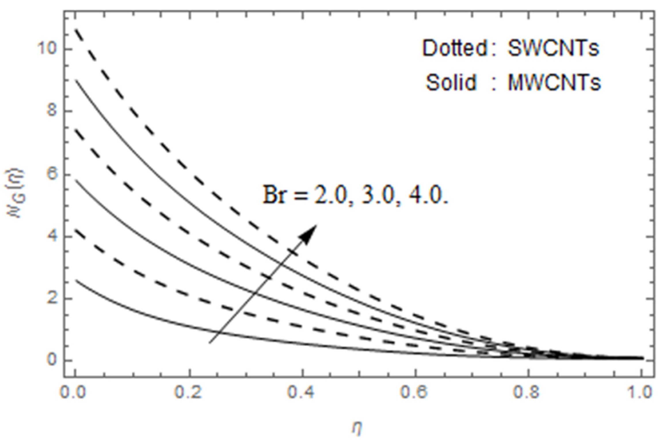
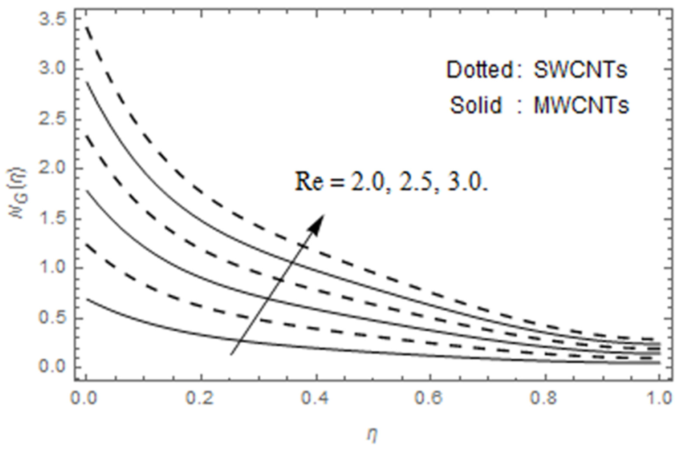
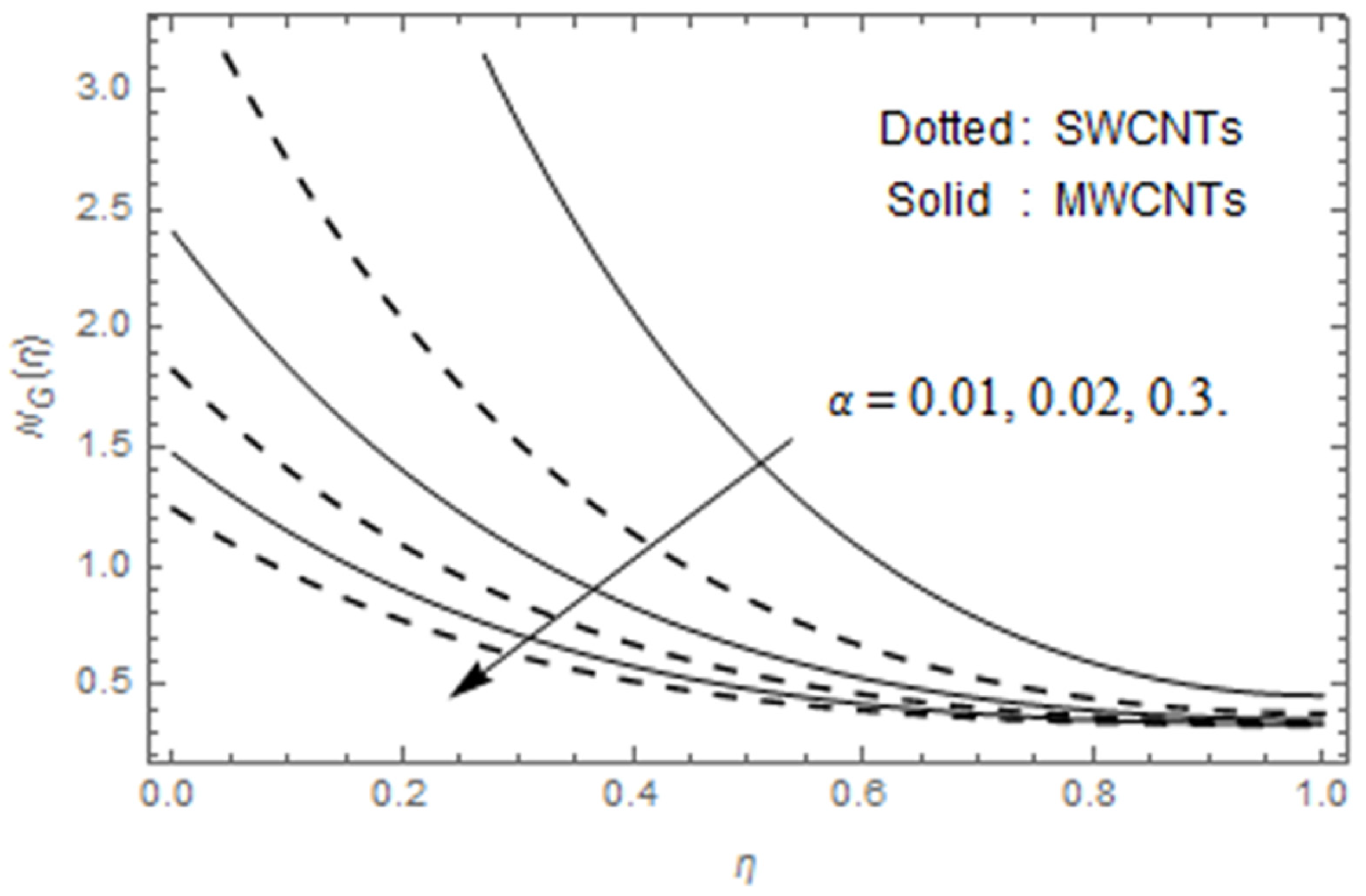
6.4. Entropy Generation

Figure 19 displays the impact of magnetic parameter $M$ on $N_G\left(\eta \right)$. The higher estimations of magnetic parameter $M$ escalate the entropy generation rate. The higher magnetic parameter effect, the greater the Lorentz force which increases the resistance of thin film fluid motion, and consequently the temperature increases. This heightens the thermal transfer rate at the wall as shown in Figure 19. Since entropy optimization $N_G\left(\eta \right)$ is a function of temperature gradient, so the robust magnetic field escalates entropy optimization $N_G\left(\eta \right)$. Figure 20 depicts the impact of Brinkman number $Br$ on entropy optimization $N_G\left(\eta \right)$. Here, entropy rate upsurges against higher estimations of Brinkman number. Actually $Br$ is a heat created source within the fluid moving region. Heat generated together with the heat transmission from the wall increases the entropy optimization. The higher Brinkman number allows less thermal conductivity to the fluid flow and therefore $N_G\left(\eta \right)$ boosted.

Figure 19. Variation in $N_G\left(\eta \right)$ via $M$.

Figure 20. Variation in $N_G\left(\eta \right)$ via $Br$.

Figure 21 displays the variation in entropy profile via Reynolds number. The higher Reynolds number escalates $N_G\left(\eta \right)$. Physically, with a higher Reynolds number, the inertial force in the system increases the viscous force which enhances the disturbance in the fluid movement and promotes an increase in entropy generation. Therefore, entropy optimization increases due to the contribution of heat transfer. Figure 22 indicates the variation in entropy generation via temperature difference parameter $\alpha$. A decreasing impact is depicted here.

Figure 21. Variation in $N_G\left(\eta \right)$ via $\mathrm{Re}$.

Figure 22. Variation in $N_G\left(\eta \right)$ via $\alpha$.

7. Conclusions

An MHD thin film flow of second grade nanofluid holding SWCNTs and MWCNTs with heat flux model of Cattaneo–Christov and entropy generation is analyzed in this article. The flow is considered past a linearly extending sheet. The final remarks of the current analysis are

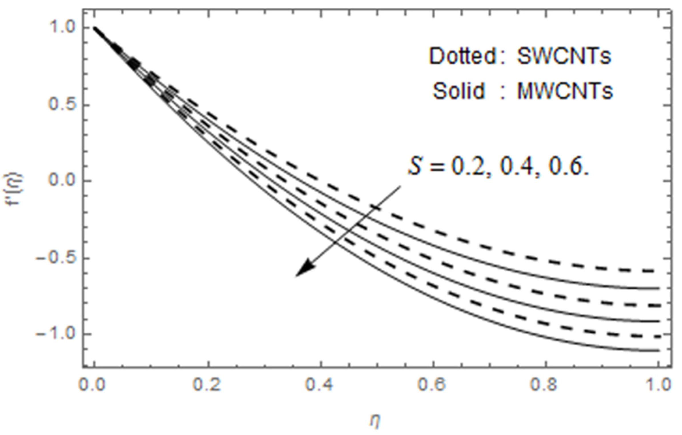
• Velocity profile heightens with the increase in nanoparticles volume fraction and second grade fluid parameter, whereas the declining impact is observed via magnetic parameter, film thickness, and unsteadiness parameter.
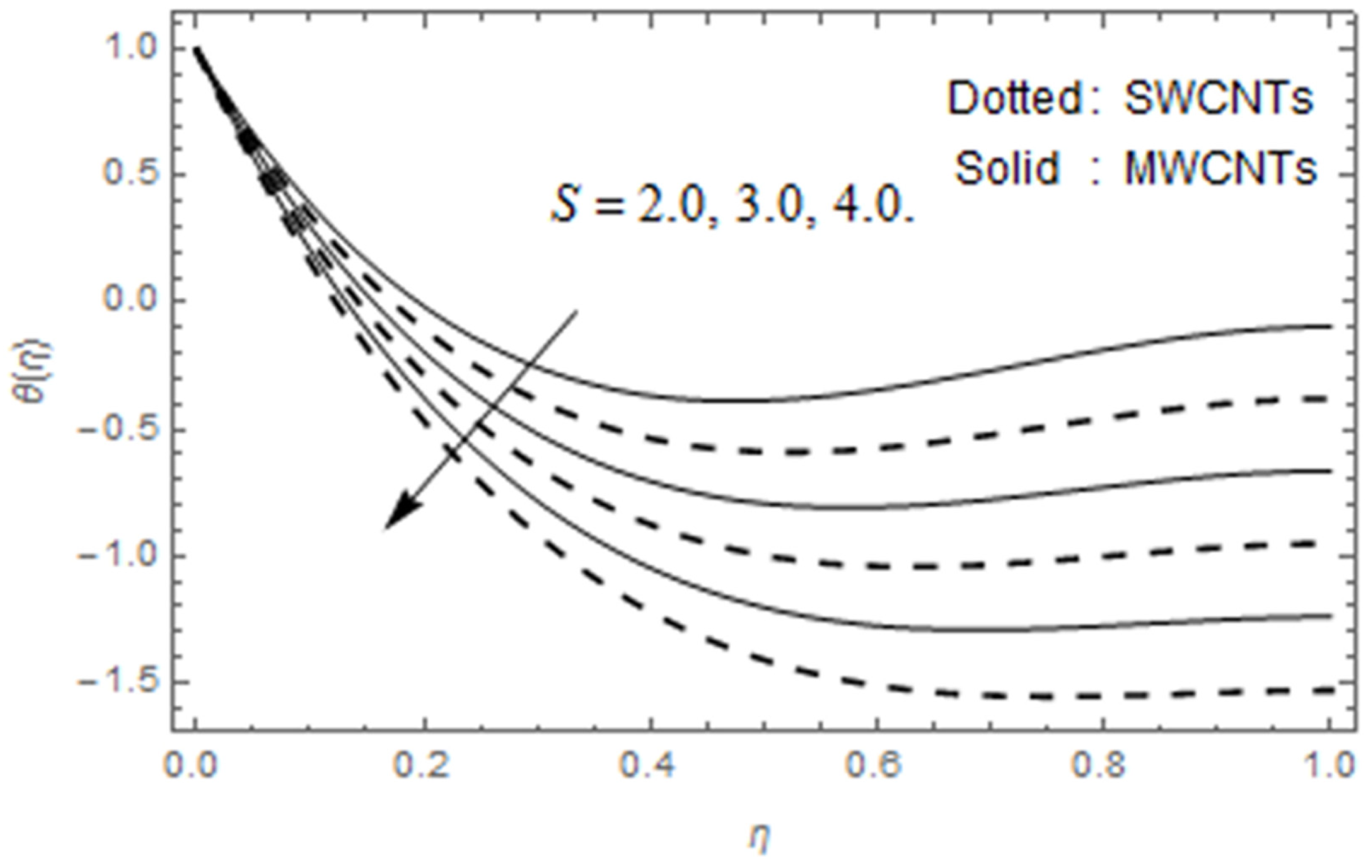
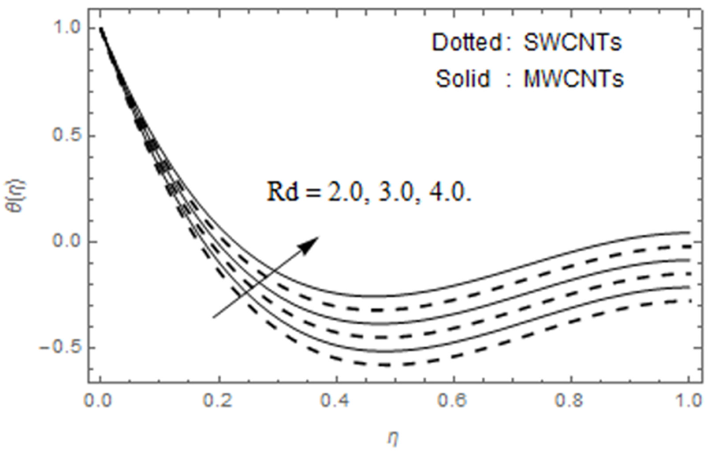
• Temperature profile heightens with the escalation in second grade fluid parameter, nanoparticles volume fraction, radiation parameter, and heat source/sink parameters while a reducing influence is observed via film thickness, unsteadiness parameter, and thermal relaxation parameter.
• Surface drag force escalates with the higher values of nanoparticles volume fraction, unsteadiness parameter, film thickness, magnetic parameter, and second grade fluid parameter.
• Thermal transfer rate surges with the heightening values of nanoparticles volume fraction, unsteadiness parameter, and film thickness, whereas a reducing effect is observed via heat source/sink parameters.
• The higher value of Reynolds number augmented the entropy optimization.
• Entropy generation increases with higer values of magnetic parameter and Brinkman number and Reynolds number.
• The entropy $N_G\left(\eta \right)$ declines with the rise of temperature difference ratio parameter.

References

1. Bertozzi, A.L.; Bowen, M. Thin Film Dynamics: Theory and Applications; Springer: Dordrecht, The Netherlands, 2002; Volume 75. [Google Scholar] [CrossRef] [Green Version]
2. Wang, C.Y. Liquid film on an unsteady stretching surface. Q. Appl. Math. 1990, 48, 601–610. [Google Scholar] [CrossRef] [Green Version]
3. Wang, C. Analytic solutions for a liquid film on an unsteady stretching surface. Heat Mass Transf. 2006, 42, 759–766. [Google Scholar] [CrossRef]
4. Andersson, H.I.; Aarseth, J.B.; Dandapat, B.S. Heat transfer in a liquid film on an unsteady stretching surface. Int. J. Heat Mass Transf. 2000, 43, 69–74. [Google Scholar] [CrossRef]
5. Liu, I.C.; Andersson, H.I. Heat transfer in a liquid film on an unsteady stretching sheet. Int. J. Therm. Sci. 2008, 47, 766–772. [Google Scholar] [CrossRef]
6. Abel, M.S.; Mahesha, N.; Tawade, J. Heat transfer in a liquid film over an unsteady stretching surface with viscous dissipation in presence of external magnetic field. Appl. Math. Model. 2009, 33, 3430–3441. [Google Scholar] [CrossRef] [Green Version]
7. Noor, N.F.M.; Abdulaziz, O.; Hashim, I. MHD flow and heat transfer in a thin liquid film on an unsteady stretching sheet by the homotopy analysis method. Int. J. Numer. Methods Fluids 2010, 63, 357–373. [Google Scholar] [CrossRef]
8. Aziz, R.C.; Hashim, I.; Alomari, A.K. Thin film flow and heat transfer on an unsteady stretching sheet with internal heating. Meccanica 2011, 46, 349–357. [Google Scholar] [CrossRef]
9. Wang, C.; Pop, I. Analysis of the flow of a power-law fluid film on an unsteady stretching surface by means of homotopy analysis method. J. Non-Newton. Fluid Mech. 2006, 138, 161–172. [Google Scholar] [CrossRef]
10. Chen, C.H. Effect of viscous dissipation on heat transfer in a non-Newtonian liquid film over an unsteady stretching sheet. J. Non-Newton. Fluid Mech. 2006, 135, 128–135. [Google Scholar] [CrossRef]
11. Chen, C.H. Marangoni effects on forced convection of power-law liquids in a thin film over a stretching surface. Phys. Lett. A 2007, 370, 51–57. [Google Scholar] [CrossRef]
12. Abbas, Z.; Hayat, T.; Sajid, M.; Asghar, S. Unsteady flow of a second-grade fluid film over an unsteady stretching sheet. Math. Comput. Model. 2008, 48, 518–526. [Google Scholar] [CrossRef]
13. Dawar, A.; Shah, Z.; Kumam, P.; Khan, W.; Islam, S. Influence of MHD on Thermal Behavior of Darcy-Forchheimer Nanofluid Thin Film Flow over a Nonlinear Stretching Disc. Coatings 2019, 9, 446. [Google Scholar] [CrossRef] [Green Version]
14. Shah, Z.; Dawar, A.; Kumam, P.; Khan, W.; Islam, S. Impact of Nonlinear Thermal Radiation on MHD Nanofluid Thin Film Flow over a Horizontally Rotating Disk. Appl. Sci. 2019, 9, 1533. [Google Scholar] [CrossRef] [Green Version]
15. Choi, S.U.; Eastman, J.A. Enhancing Thermal Conductivity of Fluids with Nanoparticles; No. ANL/MSD/CP-84938; CONF-951135-29; Argonne National Lab.: DuPage County, IL, USA, 1995. [Google Scholar]
16. Sheikholeslami, M.; Ganji, D.D. Nanofluid flow, and heat transfer between parallel plates considering Brownian motion using DTM. Comput. Methods Appl. Mech. Eng. 2015, 283, 651–663. [Google Scholar] [CrossRef]
17. Tian, X.-Y.; Li, B.-W.; Hu, Z.-M. Convective stagnation point flow of a MHD non- Newtonian nanofluid towards a stretching plate. Int. J. Heat Mass Transf. 2018, 127, 768–780. [Google Scholar] [CrossRef]
18. Abdelsalam, S.I.; Bhatti, M.M. The impact of impinging TiO2 nanoparticles in Prandtl nanofluid along with endoscopic and variable magnetic field effects on peristaltic blood flow. Multidiscip. Modeling Mater. Struct. 2018, 14, 530–548. [Google Scholar] [CrossRef]
19. Mahmood, A.; Basir, M.; Faisal, M.; Ali, U.; Mohd Kasihmuddin, M.S.; Mansor, M. Numerical Solutions of Heat Transfer for Magnetohydrodynamic Jeffery-Hamel Flow Using Spectral Homotopy Analysis Method. Processes 2019, 7, 626. [Google Scholar] [CrossRef] [Green Version]
20. Minea, A.A. Hybrid nanofluids based on Al2O3, TiO2 and SiO2: Numerical evaluation of different approaches. Int. J. Heat Mass Transf. 2017, 104, 852–860. [Google Scholar] [CrossRef]
21. Lin, Y.; Zheng, L.; Zhang, X.; Ma, L.; Chen, G. MHD pseudo-plastic nanofluid unsteady flow and heat transfer in a finite thin film over stretching surface with internal heat generation. Int. J. Heat Mass Transf. 2015, 84, 903–911. [Google Scholar] [CrossRef]
22. Lin, Y.; Zheng, L.; Chen, G. Unsteady flow and heat transfer of pseudo-plastic nanoliquid in a finite thin film on a stretching surface with variable thermal conductivity and viscous dissipation. Powder Technol. 2015, 274, 324–332. [Google Scholar] [CrossRef]
23. Zhang, Y.; Zhang, M.; Bai, Y. Flow and heat transfer of an Oldroyd-B nanofluid thin film over an unsteady stretching sheet. J. Mol. Liq. 2016, 220, 665–670. [Google Scholar] [CrossRef]
24. Zhang, Y.; Zhang, M.; Bai, Y. Unsteady flow and heat transfer of power-law nanofluid thin film over a stretching sheet with variable magnetic field and power-law velocity slip effect. J. Taiwan Inst. Chem. Eng. 2017, 70, 104–110. [Google Scholar] [CrossRef]
25. Shah, Z.; Kumam, P.; Deebani, W. Radiative MHD Casson Nanofluid Flow with Activation energy and chemical reaction over past nonlinearly stretching surface through Entropy generation. Sci. Rep. 2020, 10, 4402. [Google Scholar] [CrossRef] [PubMed] [Green Version]
26. Awais, M.; Shah, Z.; Parveen, N.; Ali, A.; Kumam, P.; Rehman, H.; Thounthong, P. MHD Effects on Ciliary-Induced Peristaltic Flow Coatings with Rheological Hybrid Nanofluid. Coatings 2020, 10, 186. [Google Scholar] [CrossRef] [Green Version]
27. Sheikholeslami, M.; Keshteli, A.N.; Houman, B. Nanoparticles favorable effects on performance of thermal storage units. J. Mol. Liq. 2020, 300, 112329. [Google Scholar] [CrossRef]
28. Oudina, F.M. Convective heat transfer of Titania nanofluids of different base fluids in cylindrical annulus with discrete heat source. Heat Transf. Asian Res. 2019, 48, 135–147. [Google Scholar] [CrossRef] [Green Version]
29. Nasir, S.; Shah, Z.; Islam, S.; Bonyah, E.; Gul, T. Darcy Forchheimer nanofluid thin film flow of SWCNTs and heat transfer analysis over an unsteady stretching sheet. AIP Adv. 2019, 9, 015223. [Google Scholar] [CrossRef] [Green Version]
30. Narayana, M.; Sibanda, P. Laminar flow of a nanoliquid film over an unsteady stretching sheet. Int. J. Heat Mass Transf. 2012, 55, 7552–7560. [Google Scholar] [CrossRef]
31. Pal, D.; Chatterjee, S. Soret and Dufour effects on MHD convective heat and mass transfer of a power-law fluid over an inclined plate with variable thermal conductivity in a porous medium. Appl. Math. Comput. 2013, 219, 7556–7574. [Google Scholar] [CrossRef]
32. Vajravelu, K.; Prasad, K.V.; Ng, C.O. Unsteady convective boundary layer flow of a viscous fluid at a vertical surface with variable fluid properties. Nonlinear Anal. Real World Appl. 2013, 14, 455–464. [Google Scholar] [CrossRef]
33. Tibullo, V.; Zampoli, V. A uniqueness result for the Cattaneo-Christov heat conduction model applied to incompressible fluids. Mech. Res. Commun. 2011, 38, 77–79. [Google Scholar] [CrossRef]
34. Han, S.; Zheng, L.; Li, C.; Zhang, X. Coupled flow and heat transfer in viscoelastic fluid with Cattaneo-Christov heat flux model. Appl. Math. Lett. 2014, 38, 87–93. [Google Scholar] [CrossRef]
35. Mustafa, M. Cattaneo-Christov heat flux model for rotating flow and heat transfer of upper-convected Maxwell fluid. AIP Adv. 2015, 5, 047109. [Google Scholar] [CrossRef]
36. Khan, J.A.; Mustafa, M.; Hayat, T.; Alsaedi, A. Numerical study of Cattaneo-Christov heat flux model for viscoelastic flow due to an exponentially stretching surface. PLoS ONE 2015, 10, e0137363. [Google Scholar]
37. Lu, D.; Li, Z.; Ramzan, M.; Shafee, A.; Chung, J.D. Unsteady squeezing carbon nanotubes based nano-liquid flow with Cattaneo-Christov heat flux and homogeneous–heterogeneous reactions. Appl. Nanosci. 2019, 9, 169–178. [Google Scholar] [CrossRef]
38. Ramzan, M.; Bilal, M.; Chung, J.D. MHD stagnation point Cattaneo-Christov heat flux in Williamson fluid flow with homogeneous–heterogeneous reactions and convective boundary condition—A numerical approach. J. Mol. Liq. 2017, 225, 856–862. [Google Scholar] [CrossRef]
39. Ramzan, M.; Bilal, M.; Chung, J.D. Influence of homogeneous-heterogeneous reactions on MHD 3D Maxwell fluid flow with Cattaneo-Christov heat flux and convective boundary condition. J. Mol. Liq. 2017, 230, 415–422. [Google Scholar] [CrossRef]
40. Ramzan, M.; Bilal, M.; Chung, J.D. Effects of MHD homogeneous-heterogeneous reactions on third grade fluid flow with Cattaneo-Christov heat flux. J. Mol. Liq. 2016, 223, 1284–1290. [Google Scholar] [CrossRef]
41. Alshomrani, A.S.; Ullah, M.Z. Effects of homogeneous–heterogeneous reactions and convective condition in Darcy–Forchheimer flow of carbon nanotubes. J. Heat Transf. 2019, 141, 012405. [Google Scholar] [CrossRef]
42. Shah, Z.; Tassaddiq, A.; Islam, S.; Alklaibi, A.M.; Khan, I. Cattaneo-Christov heat flux model for three-dimensional rotating flow of SWCNT and MWCNT nanofluid with Darcy–Forchheimer porous medium induced by a linearly stretchable surface. Symmetry 2019, 11, 331. [Google Scholar] [CrossRef] [Green Version]
43. Rivlin, R.S.; Ericksen, J.L. Stress-deformation relations for isotropic materials. J. Ration. Mech. Anal. 1955, 4, 523–532. [Google Scholar] [CrossRef]
44. Rajagopal, K.R.; Gupta, A.S. An exact solution for the flow of a non-Newtonian fluid past an infinite porous plate. Meccanica 1984, 19, 156–160. [Google Scholar] [CrossRef]
45. Alamri, S.Z.; Khan, A.A.; Azeez, M.; Ellahi, R. Effects of mass transfer on MHD second grade fluid towards stretching cylinder: A novel perspective of Cattaneo-Christov heat flux model. Phys. Lett. A 2019, 383, 276–281. [Google Scholar] [CrossRef]
46. Sandeep, N. Effect of aligned magnetic field on liquid thin film flow of magnetic-nanofluids embedded with graphene nanoparticles. Adv. Powder Technol. 2017, 28, 865–875. [Google Scholar] [CrossRef]
47. Xue, Q.Z. Model for thermal conductivity of carbon nanotube-based composites. Phys. B Condens. Matter 2005, 368, 302–307. [Google Scholar] [CrossRef]
48. Xu, H.; Pop, I.; You, X.C. Flow and heat transfer in a nano-liquid film over an unsteady stretching surface. Int. J. Heat Mass Transf. 2013, 60, 646–652. [Google Scholar] [CrossRef]