Multiple Fractional Solutions for Magnetic Bio-Nanofluid Using Oldroyd-B Model in a Porous Medium with Ramped Wall Heating and Variable Velocity

Abstract

Three different fractional models of Oldroyd-B fluid are considered in this work. Blood is taken as a special example of Oldroyd-B fluid (base fluid) with the suspension of gold nanoparticles, making the solution a biomagnetic non-Newtonian nanofluid. Based on three different definitions of fractional operators, three different models of the resulting nanofluid are developed. These three operators are based on the definitions of Caputo (C), Caputo–Fabrizio (CF), and Atnagana–Baleanu in the Caputo sense (ABC). Nanofluid is taken over an upright plate with ramped wall heating and time-dependent fluid velocity at the sidewall. The effects of magnetohydrodynamic (MHD) and porous medium are also considered. Triple fractional analysis is performed to solve the resulting three models, based on three different fractional operators. The Laplace transform is applied to each problem separately, and Zakian’s numerical algorithm is used for the Laplace inversion. The solutions are presented in various graphs with physical arguments. Results are computed and shown in various plots. The empirical results indicate that, for ramped temperature, the temperature field is highest for the ABC derivative, followed by the CF and Caputo fractional derivatives. In contrast, for isothermal temperature, the temperature field of C-derivative is higher than the CF and ABC derivatives, respectively. It was noticed that the velocity field for the ABC derivative is higher than the CF and Caputo fractional derivatives for ramped velocity. However, the velocity field for the Caputo fractional derivative is lower than the ABC and CF for isothermal velocity.

1. Introduction

Over the past few decades, nanoscience has grown to include extensive applications in engineering and medical sciences [1]. Medical science and bioengineering anticipated numerous applications of nanoscience, such as provoking the occlusion of the feeding vessels of cancer tumors, reduction of bleeding during surgeries, development of magnetic devices for cell separation, development of magnetic tracers, targeted transport of drugs using magnetic particles as drug carriers, and cancer tumor treatment causing magnetic hyperthermia [2]. One of the significant methods for cancer therapy is to set a magnetic field near to the cancer tumor or laser source insight to capture the nanoparticles, specifically gold nanoparticles, at the tumor site. The gold nanoparticles under the influence of the magnetic field or laser beam behave as a heat source [3]. The temperature of tumor cells exhibits a key role, as clarified in the hypothermia case; when heated from 42 °C to 45 °C, the cancerous tissue can be distracted. Lin et al. [4] indicated in the literature that the duration of cancer therapy can be minimized to half by improving the temperature by just 1 °C. However, the results of Misra and Shit [5] are important to clinicians as they highlighted that irreversible damage appears in the blood plasma of patients when the temperature goes above 42 °C. At that high temperature, a patient cannot survive. The dynamic of the nanoparticles injected into the blood veins is referred to as the biomagnetic fluid dynamic (BFD); the mixture of blood and nanoparticles is called bionanofluid. The bionanofluid attains motion due to peristaltic waves produced on the boundaries of blood vessels.

In 1995, the term nanofluid was highlighted by Choi and Eastman [6] for the first time. Typically, nanofluid is utilized for advanced heat transfer rate in the host fluid, which is formed by mixing nanometer-sized particles, ranging from 1 to 100 nm, in the conventional base fluid. The commonly used nanoparticles are of metals, carbides, oxides, silica, graphene, and carbon nanotubes in the general base fluid. These base fluids include oil, water, alcohol, ethylene glycol, and blood. Recently, Shah et al. [7] studied nanofluid with magnetic force and thermal trends via numerical and analytical methods. Hsiao [8] investigated nanofluid flow over a stretching surface, with viscous dissipation and magnetohydrodynamic (MHD) effects. Dianchen [9] analyzed the radiative MHD flow of nanofluid over a non-linear stretching sheet, along with homogeneous/heterogeneous chemical reactions. Zubair et al. [10] studied the 3D squeezing flow of Darcy Forchimer nanofluid, with the Cattaneo heat model and entropy generation, using four different nanoparticles. The copper and water nanofluid flow, with a heat source inside a cylindrical annulus, was numerically simulated by Oudina and Bessaïh [11]. Hatami et al. [12] analytically and numerically studied blood–gold nanofluid in a hollow vessel, under consideration of the magnetic field and porous medium. They referred third-grade fluid to blood with gold nanoparticles and followed the least square method (LSM). Tzirlakis [13] analyzed a 3D fully developed flow of Newtonian blood flow, with MHD and ferrohydrodynamic, via the finite difference method. Papadopoulos and Tzirtzilakis [14] investigated blood flow based on BFD in a curved square duct using the SIMPLE method. The results revealed that the flow could be controlled by utilizing an external magnetic field. Misra and Ghosh [15] studied blood flow in a sheet-like network connected to narrow blood vessels, referred to the lungs via the micro-continuum method. Misra et al. [16] treated blood as a non-Newtonian fluid and provided a generalized study of blood flow in a magnetic environment and porous medium. Srinivas et al. [17] analyzed the convection characteristics of blood–gold nanofluid in a microchannel with moving and static walls, under the effect of thermal radiation using the homotopy analysis method (HAM).

The above literature reveals that gold–blood nanofluid with fractional derivatives has not been reported yet. To fill this research gap, a non-Newtonian Oldroyd-B fluid model has been constructed in terms of Caputo [18], Caputo–Fabrizio (CF) [19], and Atangana–Baleanu Caputo (ABC) [20] fractional derivatives. Fractional derivatives have fascinated the significant attention of the research community over the last thirty years. The investigator recognized that discovering novel fractional derivatives, with distinct singular and nonsingular kernels, is necessary for addressing the requirements of modeling physical problems in numerous fields, such as engineering, physics, viscoelasticity, fluid mechanics, and biology [21]. To fix the singular kernel problems in Riemann–Liouville and Caputo, Caputo and Fabrizio [19] invented a novel fractional operator with the exponential kernel. However, this fractional operator faced criticism because of locality in the kernel. In connection to this, Atangana and Baleanu addressed this problem by using the generalized Mittag-Leffler function as a nonsingular and nonlocal kernel in their fractional operators in the Caputo and Riemann–Liouville sense. These fractional derivatives were used by Saad et al. [22], Morales-Delgado et al. [22], Jan et al. [23], and Gómez-Aguilar and Atangana [24]. Atangana and Gómez-Aguilar [25] investigated various models. Hence, the main objective of this study is to investigate blood–gold nanofluid with ramped velocity and temperature, using Caputo, CF, and ABC fractional derivatives. The proposed models are solved via the Laplace transform and Zakian numerical methods. The solutions are presented in numerous graphs with physical arguments.

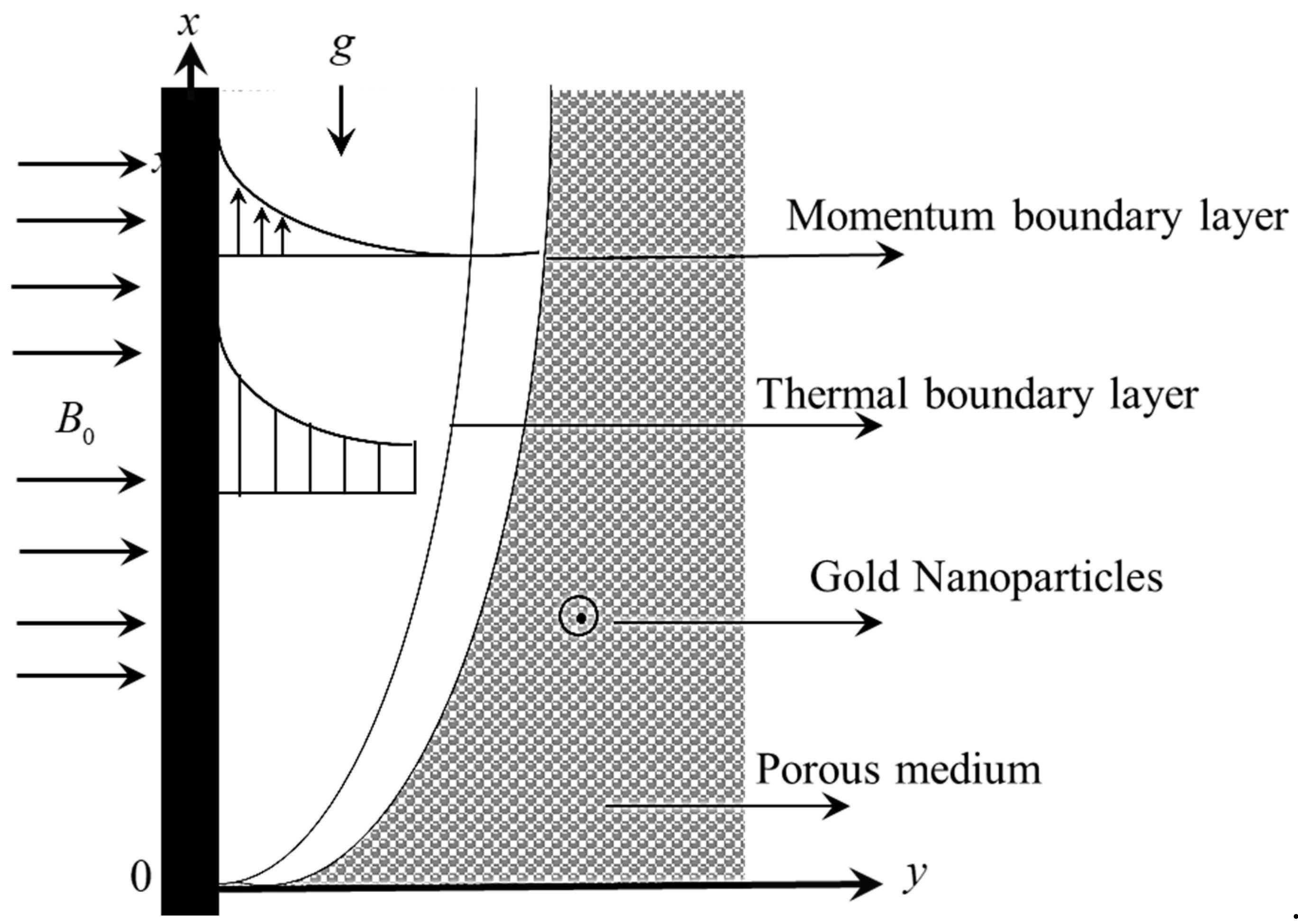
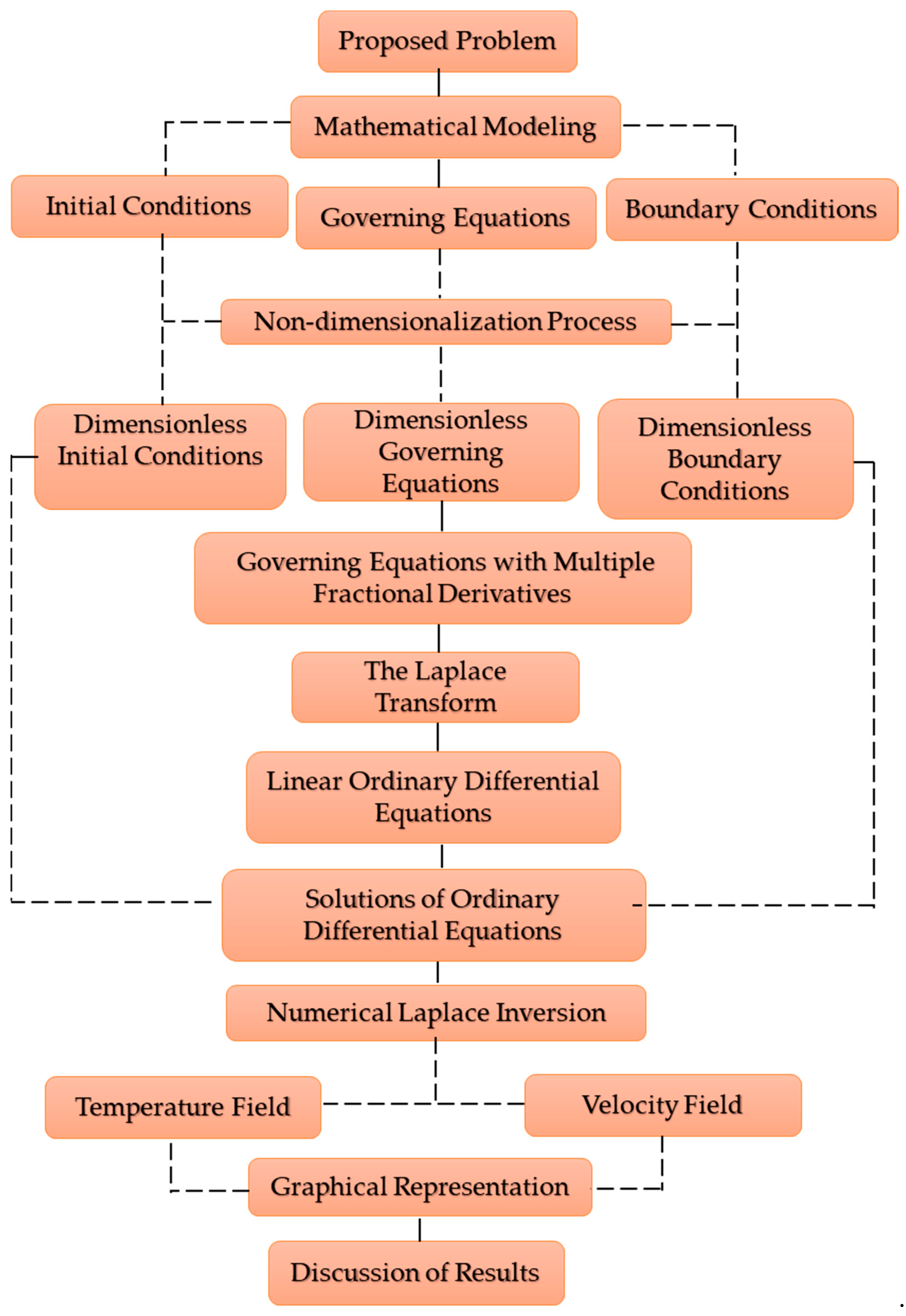
2. Mathematical Modelling

Assume the unsteady incompressible flow of an Oldroyd-B nanofluid coupled with heat transfer near an infinite plate saturated in a porous medium. The fluid is supposed to be electrically conducting; hence, an external magnetic field is employed normally to the flow direction. It is assumed that, initially, the system was at rest. However, after a short interval of time, the convection takes place because of the temperature gradient, and the fluid starts motion in the x-direction as portrayed in Figure 1.

The basic governing equations of the problem are given by [26]:

$$\nabla .\mathbf{V},$$

(1)

$${\rho }_{nf}\frac{d\mathbf{V}}{dt}=\nabla .\underset{¯}{\mathbf{T}}+\mathbf{J}\times \mathbf{B}+\mathbf{R}+\rho \mathbf{g},$$

(2)

where ${\rho }_{nf}$ is the density of nanofluid, $\mathbf{V}$ is the velocity vector, $\underset{¯}{\mathbf{T}}$ is the Cauchy stress tensor, $\mathbf{J}$ is the current density, $\mathbf{B}$ is the total magnetic field, $\mathbf{R}$ is the resistive force of porous medium, $\rho \mathbf{g}$ is the other body forces, and $d/dt$ is the material time derivative. In the case of Oldroyd-B nanofluid, the stress tensor is defined by [27]:

$$\underset{¯}{\mathbf{T}}=p\underset{¯}{\mathbf{I}}+\underset{¯}{\mathbf{S}},$$

(3)

$$\underset{¯}{\mathbf{S}}+\lambda \frac{D\underset{¯}{\mathbf{S}}}{Dt}={\mu }_{nf}\left(1+{\lambda }_r\frac{D}{Dt}\right){\underset{¯}{\mathbf{A}}}_1,$$

(4)

where $\underset{¯}{\mathbf{T}}$ is already defined, $p$ is the pressure, $\underset{¯}{\mathbf{I}}$ is the identity tensor, $\underset{¯}{\mathbf{S}}$ is the extra stress, $\lambda$ is the time of relaxation, $D/Dt$ is the convective time derivative, ${\mu }_{nf}$ is the dynamic viscosity of nanofluid, ${\lambda }_r$ is the retardation time, and ${\underset{¯}{\mathbf{A}}}_1$ is the first kind of Rivlin–Ericksen tensor. Using the Maxwells’ set of equations and Darcy resistance, the terms $\mathbf{J}\times \mathbf{B}$ and $\mathbf{R}$ are defined in the following form [28,29]:

$$\mathbf{J}\times \mathbf{B}=-{\sigma }_{nf}{B}_0^2\mathbf{V},$$

(5)

$$\left(1+\lambda \frac{\partial }{\partial t}\right)\mathbf{R}=-\frac{{\mu }_{nf}\varphi }{k}\left(1+{\lambda }_r\frac{\partial }{\partial t}\right)\mathbf{V},$$

(6)

where ${\sigma }_{nf}$ is the electrical conductivity of nanofluid, $B_0$ is the magnetic field, $\phi ;0<\phi <1$ is the porosity, and $k$ is the permeability of the porous medium. In the case of the present problem, the velocity vector $\mathbf{V}$ and extra stress $\underset{¯}{\mathbf{S}}$ are chosen in the following form.

$$\mathbf{V}=\left\{u(y,t),0,0\right\}\hspace{0.17em},\underset{¯}{\mathbf{S}}=\underset{¯}{\mathbf{S}}(y,t)$$

(7)

After the settlement of Equations (3)–(7) subject to $\mathbf{S}(y,0)\Rightarrow S_{yy}=S_{yz}=S_{zx}=S_{zz}=0$ and using the Boussinesq approximation the governing equation of Oldroyd nanofluid yield:

$$\begin{array}{ll}{\rho }_{nf}\left(1+\lambda \frac{\partial }{\partial t}\right)\frac{\partial u(y,t)}{\partial t}=& \left({\mu }_{nf}+{\mu }_{nf}{\lambda }_r\frac{\partial }{\partial t}\right)\frac{{\partial }^{2}u(y,t)}{\partial y^2}-{\sigma }_{nf}{B}_0^2\left\{u(y,t)+\lambda \frac{\partial u(y,t)}{\partial t}\right\}\\ & -\left\{\frac{{\mu }_{nf}\varphi }{k}u(y,t)+\frac{{\mu }_{nf}\varphi }{k}{\lambda }_r\frac{\partial u(y,t)}{\partial t}\right\}+g{(\rho {\beta }_T)}_{nf}(T(y,t)-T_{\infty }),\end{array}$$

(8)

$${(\rho C_p)}_{nf}\frac{\partial T(y,t)}{\partial t}=k_{nf}\frac{{\partial }^{2}T(y,t)}{\partial y^2}$$

(9)

where $g$ is gravitational acceleration, ${({\beta }_T)}_{nf}$ is the thermal expansion of nanofluid, $T(y,t)$ is the temperature, ${(C_p)}_{nf}$ is the heat capacitance, and $k_{nf}$ is the thermal conductivity of nanofluid, and ${\rho }_{nf}$, $\lambda$, $u(y,t)$, ${\mu }_{nf}$, ${\sigma }_{nf}$, $B_0$ and ${\lambda }_r$ were previously defined. Equations (8) and (9) are subject to the following initial and ramped wall boundary [30]

$$u(y,0)=0,\hspace{0.17em}T(y,0)=T_{\infty },\hspace{0.17em}\forall y\ge 0,$$

(10)

$$\begin{array}{l}\begin{array}{l}u(0,t)=\{\begin{array}{ll}{u}_0\frac{t}{t_0}& ;\mathrm{if}\hspace{0.17em}0<t<t_0\\ u_0& ;\hspace{0.17em}\mathrm{if}\hspace{0.17em}t>t_0\end{array}\\ T(0,t)=\{\begin{array}{ll}{T}_0+(T_W-T_{\infty })\frac{t}{t_0}& ;\hspace{0.17em}\mathrm{if}\hspace{0.17em}0<t<t_0\\ T_W& ;\hspace{0.17em}\mathrm{if}\hspace{0.17em}t>t_0\end{array}\end{array}\},\\ u(y,t)\to 0 \mathrm{and} T(y,t)\to T_{\infty };\hspace{0.17em}\mathrm{if}\hspace{0.17em}y\to \infty .\end{array}$$

(11)

The mathematical expressions for the thermophysical properties of nanofluid are taken to be of the following form [28]:

$$\begin{array}{l}{\rho }_{nf}=(1-\varphi ){\rho }_f+\varphi {\rho }_s,{\mu }_{nf}=\frac{{\mu }_f}{{(1-\varphi )}^{2.5}},\frac{{\sigma }_{nf}}{{\sigma }_f}=1+\frac{3\left(\frac{{\sigma }_s}{{\sigma }_f}-1\right)\varphi }{\left(\frac{{\sigma }_s}{{\sigma }_f}+2\right)-\left(\frac{{\sigma }_s}{{\sigma }_f}-1\right)\varphi },{(\rho {\beta }_T)}_{nf}=(1-\varphi )\\ \times {(\rho {\beta }_T)}_f+\varphi {(\rho {\beta }_T)}_s,{(\rho C_p)}_{nf}=(1-\varphi ){(\rho C_p)}_f+\varphi {(\rho C_p)}_s,\frac{k_{nf}}{k_f}=\frac{k_s+2k_f+2\varphi (k_s-k_f)}{k_s+2k_f-\varphi (k_s-k_f)}\end{array}\}.$$

(12)

In Equation (12), the subscripts $nf$, $f$, and $s$ represent o nanofluid, base fluid, and solid nanoparticles. For the present problem, blood is chosen as a non-Newtonian base fluid and gold nanoparticles are dispersed into it to form nanofluid. The thermophysical numerical values of blood and gold nanoparticles are given in

Table 1. Numerical values of base fluid and solid material nanoparticles [31,32,33].

Material	Base Fluid	Nanoparticles
	Blood	Gold
$\rho (\mathrm{kg}/{\mathrm{m}}^3)$	1053	1250
$C_p(\mathrm{J}/\mathrm{kg}\hspace{0.17em}\mathrm{K})$	3594	129
$k(\mathrm{W}/\mathrm{m}\hspace{0.17em}\mathrm{K})$	0.492	318
${\beta }_T\times {10}^{-5}({\mathrm{K}}^{-1})$	0.8	1.41
$\sigma$	0.18	4.45 × 107
Pr	21	-

.

3. Derivation of Fractional Model for Blood–Gold Nanofluid

Firstly, Equations (8)–(11) will be transformed to dimensionless form. For this purpose, the following dimensionless variables:

$$f=\frac{u}{u_0},\xi =\frac{u_0}{{\upsilon }_f}y,\tau =\frac{t}{t_0},t_0=\frac{{\upsilon }_f}{u_0^2},\Phi =\frac{T-T_{\infty }}{T_W-T_{\infty }}$$

are incorporated into Equations (8)–(11) to yield:

$$\begin{array}{l}{\varphi }_0\left\{\frac{\partial f(\xi ,\tau )}{\partial \tau }+{\lambda }_1\frac{{\partial }^{2}f(\xi ,\tau )}{\partial {\tau }^2}\right\}={\varphi }_1\left\{\frac{{\partial }^{2}f(\xi ,\tau )}{\partial {\xi }^2}+{\lambda }_2\frac{{\partial }^{3}f(\xi ,\tau )}{\partial \tau \partial {\xi }^2}\right\}\\ -{\varphi }_{2}M\left\{f(\xi ,\tau )+{\lambda }_1\frac{\partial f(\xi ,\tau )}{\partial \tau }\right\}-\frac{{\varphi }_1}{K}\left\{f(\xi ,\tau )+{\lambda }_2\frac{\partial f(\xi ,\tau )}{\partial \tau }\right\}+{\varphi }_{3}Gr\theta (y,t)\end{array}$$

(13)

$${\varphi }_4\frac{\partial \Phi (\xi ,\tau )}{\partial \tau }=\frac{{\varphi }_5}{\mathrm{Pr}}\frac{{\partial }^2\Phi (\xi ,\tau )}{\partial {\xi }^2}$$

(14)

and

$$f(\xi ,0)=0,\Phi (\xi ,0)=0,\hspace{0.17em}\forall \xi \ge 0$$

(15)

$$\begin{array}{l}\begin{array}{l}f(0,\tau )=\{\begin{array}{ll}\tau ;& \mathrm{if}\hspace{0.17em}0<\tau <1\\ 1;& \mathrm{if}\hspace{0.17em}\tau >1\end{array}\\ \Phi (0,\tau )=\{\begin{array}{ll}\tau ;& \mathrm{if}\hspace{0.17em}0<\tau <1\\ 1;& \mathrm{if}\hspace{0.17em}\tau >1\end{array}\end{array}\}\\ f(\xi ,\tau )\to 0\hspace{0.17em}\mathrm{and}\hspace{0.17em}T(\xi ,\tau )\to 0;\mathrm{if}\hspace{0.17em}\xi \to \infty \end{array}$$

(16)

where:

$$\begin{gathered} {\lambda }_1=\frac{\lambda }{t_0}, {\lambda }_2=\frac{{\lambda }_r}{t_0}, M=\frac{t_0{\sigma }_f{B}_0^2}{{\rho }_f}, K=\frac{k}{t_0{\upsilon }_f\varphi } Gr=\frac{g{({\beta }_T\upsilon )}_f(T_W-T_{\infty })}{u_0^3}, \mathrm{Pr}={\left(\frac{\mu C_p}{k}\right)}_f, {\varphi }_0=(1-\varphi )+\varphi \frac{{\rho }_s}{{\rho }_f}, \\ {\varphi }_1=\frac{1}{{(1-\varphi )}^{2.5}}, {\varphi }_2=\frac{{\sigma }_{nf}}{{\sigma }_f}, {\varphi }_3=(1-\varphi )+\varphi \frac{{(\rho {\beta }_T)}_s}{{(\rho {\beta }_T)}_f}, {\varphi }_4=(1-\varphi )+\varphi \frac{{(\rho C_p)}_s}{{(\rho C_p)}_f}, {\varphi }_5=\frac{k_{nf}}{k_f} \end{gathered}$$

are the dimensionless relaxation time, retardation time, magnetic number, permeability of the porous medium, thermal Grashof number, and Prandtl number, respectively. In addition to this, ${\varphi }_0$, ${\varphi }_1$, ${\varphi }_2$, ${\varphi }_3$, ${\varphi }_4$ and ${\varphi }_5$ are constant terms that appeared during calculations. Now, the Caputo fractional derivative with the Laplace transform (LT) is given by [18,34].

$${}^C{D}_{\tau }^{\delta }g(\xi ,\tau )=\frac{1}{\Gamma (n-\delta )}{\displaystyle \underset{0}{\overset{\tau }{\int }}\frac{g^{(n)}(\xi ,\tau )}{{(\tau -s)}^{\delta +1-n}}}ds,$$

(17)

$$ℒ\left\{{}^C{D}_{\tau }^{\delta }g(\xi ,\tau )\right\}(q)=\overline{g}(\xi ,q)=q^{\delta }ℒ\left\{g(\xi ,\tau )\right\}-q^{\delta -1}g(\xi ,0),$$

(18)

where $D_{\tau }^{\delta }g(\xi ,\tau )$ is the Caputo fractional derivative, $\delta$ is the fractional-order, and $\Gamma (.)$ is the gamma function. The kernel of Caputo fractional derivatives is singular for $\tau =s$. The Caputo–-Fabrizio (CF) fractional derivative without singular kernel and its LT is given by [19].

$${}^{CF}{D}_{\tau }^{\delta }g(\xi ,\tau )=\frac{1}{n-\delta }{\displaystyle \underset{0}{\overset{\tau }{\int }}\exp \left(-\frac{\delta (\delta -\tau )}{1-\delta }\right)\frac{\partial g(\xi ,s)}{\partial s}}ds,$$

(19)

$$ℒ\left\{{}^{CF}{D}_{\tau }^{\delta }g(\xi ,\tau )\right\}(q)=\overline{g}(\xi ,q)=\frac{qℒ\left\{g(\xi ,\tau )\right\}-g(\xi ,\tau )}{(1-\delta )q+\delta },$$

(20)

with local exponential kernel and order $\delta$. The Atangana–Baleanu Caputo (ABC) fractional derivative, without singularity and locality with its LT, is given by [20].

$${}^{ABC}{D}_{\tau }^{\delta }g(\xi ,\tau )=\frac{1}{n-\delta }{\displaystyle \underset{0}{\overset{\tau }{\int }}{E}_{\delta }\left(-\frac{\delta {(\delta -\tau )}^{\delta }}{1-\delta }\right)\frac{\partial g(\xi ,s)}{\partial s}}ds,$$

(21)

$$ℒ\left\{{}^{ABC}{D}_{\tau }^{\delta }g(\xi ,\tau )\right\}(q)=\overline{g}(\xi ,q)=\frac{q^{\delta }ℒ\left\{g(\xi ,\tau )\right\}-q^{\delta -1}g(\xi ,\tau )}{(1-\delta )q^{\delta }+\delta }.$$

(22)

Kernel of Atangana–Baleanu Caputo derivative is a generalized Mittag-Leffler function without singularity and locality. In the following section, the problem presented in Equations (13)–(16) will be solved using Equations (17)–(22).

4. Solutions to the Problem

In this section, the proposed problem will be solved in terms of Caputo, CF, and ABC fractional derivatives. The dimensionless problem is transformed into multiple fractional derivatives and solved using the joint Laplace transform and Zakian’s numerical algorithm, as depicted in Figure 2.

4.1. Solution Temperature Field Based on Caputo Fractional Derivative

The energy equation (Equation (14)) in terms of Caputo fractional derivatives is derived by using Equation (17) as:

$${\varphi }_4\mathrm{Pr}{\hspace{0.17em}}^C{D}_{\tau }^{\alpha }\Phi (\xi ,\tau )={\varphi }_1\frac{{\partial }^2\Phi (\xi ,\tau )}{\partial y^2},$$

(23)

where ${}^C{D}_{\tau }^{\alpha }\Phi (\xi ,\tau )$ is the Caputo fractional derivative of the dimensionless temperature $\Phi (\xi ,\tau )$ and $\alpha$ is the fractional order. Applying the LT to Equation (23) using Equation (18) yields:

$$\frac{d^2\overline{\Phi }(\xi ,\tau )}{\partial {\xi }^2}-a_0{q}^{\alpha }\overline{\Phi }(\xi ,\tau )=0,$$

(24)

with the corresponding transformed boundary condition:

$$\overline{\Phi }(0,\tau )=\frac{(1-e^{-q})}{q^2},\overline{\Phi }(\infty ,\tau )=0,$$

(25)

where:

$$a_0=\frac{{\varphi }_4\mathrm{Pr}}{{\varphi }_5}.$$

Equation (24) is analytically solved, and the transform boundary conditions from Equation (25) are used, which yield:

$$\overline{\Phi }(\psi ,\tau )=\frac{1}{q^2}{e}^{-\xi \sqrt{a_0{q}^{\alpha }}}-\frac{e^{-q}}{q^2}{e}^{-\xi \sqrt{a_0{q}^{\alpha }}}.$$

(26)

4.2. Solution for Temperature Field Based on CF Fractional Derivative

Equation (19) is used to transform Equation (14) in the CF fractional derivative sense as:

$${\varphi }_4\mathrm{Pr}{\hspace{0.17em}}^{CF}{D}_{\tau }^{\alpha }\Phi (\xi ,\tau )={\varphi }_1\frac{{\partial }^2\Phi (\xi ,\tau )}{\partial y^2}.$$

(27)

Keeping in view Equation (20), the LT of Equation (27) is obtained as:

$$\frac{d^2\overline{\Phi }(\xi ,\tau )}{\partial {\xi }^2}-\frac{a_{0}q}{(1-\alpha )q+\alpha }\overline{\Phi }(\xi ,\tau )=0.$$

(28)

Equation (28) is analytically solved, and the transform boundary conditions from Equation (25) are used, which yield:

$$\overline{\Phi }(\xi ,\tau )=\frac{1}{q^2}{e}^{-\xi \sqrt{\frac{a_{0}q}{(1-\alpha )q+\alpha }}}-\frac{e^{-q}}{q^2}{e}^{-\xi \sqrt{\frac{a_{0}q}{(1-\alpha )q+\alpha }}}.$$

(29)

4.3. Solution for Temperature Field Based on ABC Fractional Derivative

To develop the energy equation in ABC form, Equation (21) is used, which transforms Equation (14) into the following form:

$${\varphi }_4\mathrm{Pr}{\hspace{0.17em}}^{ABC}{D}_{\tau }^{\alpha }\Phi (\xi ,\tau )={\varphi }_1\frac{{\partial }^2\Phi (\xi ,\tau )}{\partial y^2}.$$

(30)

The LT of Equation (30) in the light of Equation (22) is obtained as:

$$\frac{d^2\overline{\Phi }(\xi ,\tau )}{\partial {\xi }^2}-\frac{a_0{q}^{\alpha }}{(1-\alpha )q^{\alpha }+\alpha }\overline{\Phi }(\xi ,\tau )=0.$$

(31)

Equation (31) is analytically solved and the transform boundary conditions from Equation (25) are used, which yield:

$$\overline{\Phi }(\xi ,\tau )=\frac{1}{q^2}{e}^{-\xi \sqrt{\frac{a_0{q}^{\alpha }}{(1-\alpha )q^{\alpha }+\alpha }}}-\frac{e^{-q}}{q^2}{e}^{-\xi \sqrt{\frac{a_0{q}^{\alpha }}{(1-\alpha )q^{\alpha }+\alpha }}}.$$

(32)

4.4. Solutions for Velocity Field Based on Caputo Fractional Derivative

The momentum equations (Equation (13)) are transformed in terms of the Caputo fractional derivative as:

$$\begin{array}{l}{\varphi }_0\left\{{}^C{D}_{\tau }^{\alpha }f(\xi ,\tau )+{\lambda }_1{\hspace{0.17em}}^C{D}_{\tau }^{2\alpha }f(\xi ,\tau )\right\}={\varphi }_1\left\{\frac{{\partial }^{2}f(\xi ,\tau )}{\partial {\xi }^2}+{\lambda }_2{}^C{D}_{\tau }^{\beta }\frac{{\partial }^{2}f(\xi ,\tau )}{\partial {\xi }^2}\right\}\\ -{\varphi }_{2}M\left\{f(\xi ,\tau )+{\lambda }_1{}^C{D}_{\tau }^{\alpha }f(\xi ,\tau )\right\}-\frac{{\varphi }_1}{K}\left\{f(\xi ,\tau )+{\lambda }_2{}^C{D}_{\tau }^{\beta }f(\xi ,\tau )\right\}+{\varphi }_{3}Gr\Phi (\xi ,\tau )\end{array}$$

(33)

For convenience in the solution, Equation (33) is re-arranged and organized as:

$$\begin{array}{l}\frac{{\varphi }_0}{{\varphi }_1}{\left\{1+{\lambda }_1{}^C{D}_{\tau }^{\alpha }\hspace{0.17em}\right\}}^C{D}_{\tau }^{\alpha }f(\xi ,\tau )+\frac{{\varphi }_2}{{\varphi }_1}M\left\{1+{\lambda }_1{}^C{D}_{\tau }^{\alpha }\right\}f(\xi ,\tau )\\ =\left\{1+{\lambda }_2{}^C{D}_{\tau }^{\beta }\right\}\frac{{\partial }^{2}f(\xi ,\tau )}{\partial {\xi }^2}-\frac{1}{K}\left\{1+{\lambda }_2{}^C{D}_{\tau }^{\beta }\right\}f(\xi ,\tau )+G{r}_0\Phi (\xi ,\tau )\end{array}$$

(34)

where:

$$G{r}_0=\frac{{\varphi }_3}{{\varphi }_1}Gr.$$

Employing the LT in Equation (34), in accordance with Equation (18), yields:

$$\begin{array}{l}\frac{{\varphi }_0}{{\varphi }_1}\left\{1+{\lambda }_1{q}^{\alpha }\hspace{0.17em}\right\}{q}^{\alpha }\overline{f}(\xi ,q)+\frac{{\varphi }_2}{{\varphi }_1}M\left\{1+{\lambda }_1{q}^{\alpha }\right\}\overline{f}(\xi ,q)=\\ \left\{1+{\lambda }_2{q}^{\beta }\right\}\frac{{\partial }^2\overline{f}(\xi ,q)}{\partial {\xi }^2}-\frac{1}{K}\left\{1+{\lambda }_2{q}^{\beta }\right\}\overline{f}(\xi ,q)+G{r}_0\overline{\Phi }(\xi ,q)\end{array}$$

(35)

Incorporating Equation (26) into Equation (35) leads to the following form:

$$\frac{d^2\overline{f}(\xi ,q)}{d{\xi }^2}-\frac{(1+{\lambda }_1{q}^{\alpha })({\varphi }_{2}M+{\varphi }_0{q}^{\alpha })}{{\varphi }_1(1+{\lambda }_2{q}^{\beta })}\overline{f}(\xi ,q)-\frac{\overline{f}(\xi ,q)}{K}=-\frac{G{r}_0(1-e^q)}{q^2}{e}^{-\xi \sqrt{a_0{q}^{\alpha }}},$$

(36)

with the corresponding transformed boundary condition:

$$\overline{f}(0,\tau )=\frac{(1-e^{-q})}{q^2},\hspace{0.17em}\overline{f}(\infty ,\tau )=0.$$

(37)

Using the boundary conditions from Equation (37), the exact analytical solution of Equation (36) in the LT domain is given by:

$$\overline{f}(\xi ,q)=\left\{\frac{(1-e^{-q})}{q^2}+{\Theta }_0(q)\right\}{e}^{-\xi \sqrt{\frac{(1+{\lambda }_1{q}^{\alpha })({\varphi }_{2}M+{\varphi }_0{q}^{\alpha })}{{\varphi }_1(1+{\lambda }_2{q}^{\beta })}+\frac{1}{K}}}-{\Theta }_0(q)e^{-\xi \sqrt{a_0{q}^{\alpha }}},$$

(38)

where:

$${\Theta }_0(q)=\frac{G{r}_0{\varphi }_{1}K(1+{\lambda }_2{q}^{\beta })(1-e^{-q})}{q^2\left\{a_0{\varphi }_1{q}^{\alpha }K(1+{\lambda }_2{q}^{\beta })-K(1+{\lambda }_1{q}^{\alpha })({\varphi }_{2}M+{\varphi }_0{q}^{\alpha })-{\varphi }_1(1+{\lambda }_2{q}^{\beta })\right\}}.$$

4.5. Solutions for Velocity Field Based on CF Fractional Derivative

The CF fractional form of Equation (13) is given by:

$$\begin{array}{l}\frac{{\varphi }_0}{{\varphi }_1}\left\{1+{\lambda }_1{}^{CF}{D}_{\tau }^{\alpha }\hspace{0.17em}\right\}{\hspace{0.17em}}^{CF}{D}_{\tau }^{\alpha }f(\xi ,\tau )+\frac{{\varphi }_2}{{\varphi }_1}M\left\{1+{\lambda }_1{\hspace{0.17em}}^{CF}{D}_{\tau }^{\alpha }\right\}f(\xi ,\tau )\\ =\left\{1+{\lambda }_2{\hspace{0.17em}}^{CF}{D}_{\tau }^{\beta }\right\}\frac{{\partial }^{2}f(\xi ,\tau )}{\partial {\xi }^2}-\frac{1}{K}\left\{1+{\lambda }_2{\hspace{0.17em}}^{CF}{D}_{\tau }^{\beta }\right\}f(\xi ,\tau )+G{r}_0\Phi (\xi ,\tau )\end{array}$$

(39)

Applying the LT to Equation (39) using Equation (20) yields:

$$\begin{array}{l}\frac{{\varphi }_0}{{\varphi }_1}\left\{1+\frac{{\lambda }_{1}q}{(1-\alpha )q+\alpha }\hspace{0.17em}\right\}\hspace{0.17em}\frac{q\overline{f}(\xi ,q)}{(1-\alpha )q+\alpha }+\frac{{\varphi }_2}{{\varphi }_1}M\left\{1+\frac{{\lambda }_{1}q}{(1-\alpha )q+\alpha }\hspace{0.17em}\right\}f(\xi ,\tau )\\ =\left\{1+\frac{{\lambda }_{2}q}{(1-\beta )q+\beta }\hspace{0.17em}\right\}\frac{d^2\overline{f}(\xi ,q)}{d{\xi }^2}-\frac{1}{K}\left\{1+\frac{{\lambda }_{2}q}{(1-\beta )q+\beta }\right\}\overline{f}(\xi ,q)+G{r}_0\overline{\Phi }(\xi ,q)\end{array}$$

(40)

Introducing Equation (29) into Equation (40) yields:

$$\frac{d^2\overline{f}(\xi ,q)}{d{\xi }^2}-\frac{{\varphi }_{0}q{\Theta }_1(q)+{\varphi }_{2}M\left\{(1-\alpha )q+\alpha \right\}{\Theta }_1(q)}{{\varphi }_1{\Theta }_2(q)\left\{(1-\alpha )q+\alpha \right\}}\overline{f}(\xi ,q)-\frac{1}{K}\overline{f}(\xi ,q)=-G{r}_0(\frac{1-e^{-q}}{q^2})e^{-\xi \sqrt{\frac{a_{0}q}{(1-\alpha )q+\alpha }}},$$

(41)

where:

$${\Theta }_1(q)=\frac{(1-\alpha +{\lambda }_1)q+\alpha }{(1-\alpha )q+\alpha }, {\Theta }_2(q)=\frac{(1-\beta +{\lambda }_2)q+\beta }{(1-\beta )q+\beta }.$$

Using the boundary conditions from Equation (37), the exact solution of Equation (41) is given by:

$$\overline{f}(\xi ,q)=\left\{\frac{(1-e^{-q})}{q^2}+{\Theta }_3(q)e^{-\xi \sqrt{{\Theta }_1(q)\frac{{\varphi }_{0}q+{\varphi }_{2}M\left\{(1-\alpha )q+\alpha \right\}}{{\varphi }_1{\Theta }_2(q)\left\{(1-\alpha )q+\alpha \right\}}-\frac{1}{K}}}\right\}-{\Theta }_3(q)e^{-\xi \sqrt{\frac{a_{0}q}{(1-\alpha )q+\alpha }}},$$

(42)

where:

$${\Theta }_3(q)=\frac{G{r}_{0}K{\varphi }_1(1-e^{-q})\left\{(1-\alpha )q+\alpha \right\}{\Theta }_2(q)}{q^2\left[K{\varphi }_1{a}_{0}q{\Theta }_2(a)-{\varphi }_1\left\{(1-\alpha )q+\alpha \right\}{\Theta }_2(a)-K{\varphi }_{0}q{\Theta }_1(q)-K{\varphi }_{2}M\left\{(1-\alpha )q+\alpha \right\}{\Theta }_1(q)\right]}.$$

4.6. Solutions for Velocity Field Based on Atangana–Baleanu–Caputo Fractional Derivative

ABC fractional form Equation (13) is constructed by using Equation (21) as:

$$\begin{array}{l}\frac{{\varphi }_0}{{\varphi }_1}\left\{1+{\lambda }_1{\hspace{0.17em}}^{ABC}{D}_{\tau }^{\alpha }\hspace{0.17em}\right\}\hspace{0.17em}{\hspace{0.17em}}^{ABC}{D}_{\tau }^{\alpha }f(\xi ,\tau )+\frac{{\varphi }_2}{{\varphi }_1}M\left\{1+{\lambda }_1{\hspace{0.17em}}^{ABC}{D}_{\tau }^{\alpha }\right\}f(\xi ,\tau )\\ =\left\{1+{\lambda }_2{\hspace{0.17em}}^{ABC}{D}_{\tau }^{\beta }\right\}\frac{{\partial }^{2}f(\xi ,\tau )}{\partial {\xi }^2}-\frac{1}{K}\left\{1+{\lambda }_2{\hspace{0.17em}}^{ABC}{D}_{\tau }^{\beta }\right\}f(\xi ,\tau )+G{r}_0\Phi (\xi ,\tau )\end{array}$$

(43)

Employing the LT to Equation (43), in the view of Equation (22), yields:

$$\begin{array}{l}\frac{{\varphi }_0}{{\varphi }_1}\left\{1+\hspace{0.17em}\frac{{\lambda }_1{q}^{\alpha }}{(1-\alpha )q^{\alpha }+\alpha }\hspace{0.17em}\right\}\hspace{0.17em}\hspace{0.17em}\frac{q^{\alpha }\overline{f}(\xi ,q)}{(1-\alpha )q^{\alpha }+\alpha }+\frac{{\varphi }_2}{{\varphi }_1}M\left\{1+\hspace{0.17em}\frac{{\lambda }_1{q}^{\alpha }}{(1-\alpha )q^{\alpha }+\alpha }\right\}\overline{f}(\xi ,q)=\\ \left\{1+\frac{{\lambda }_2{q}^{\beta }}{(1-\beta )q^{\beta }+\beta }\right\}\frac{d^2\overline{f}(\xi ,q)}{d{\xi }^2}-\frac{1}{K}\left\{1+\frac{{\lambda }_2{q}^{\beta }}{(1-\beta )q^{\beta }+\beta }\right\}\overline{f}(\xi ,q)+G{r}_0\overline{\Phi }(\xi ,q)\end{array}$$

(44)

Incorporating Equation (32) into Equation (44) yields:

$$\frac{d^2\overline{f}(\xi ,q)}{d{\xi }^2}-\frac{{\varphi }_{0}q{\Theta }_4(q)+{\varphi }_{2}M\left\{(1-\alpha )q^{\alpha }+\alpha \right\}{\Theta }_4(q)}{{\varphi }_1{\Theta }_5(q)\left\{(1-\alpha )q^{\alpha }+\alpha \right\}}\overline{f}(\xi ,q)-\frac{\overline{f}(\xi ,q)}{K}=-G{r}_0(\frac{1-e^{-q}}{q^2})e^{-\xi \sqrt{\frac{a_0{q}^{\alpha }}{(1-\alpha )q^{\alpha }+\alpha }}}$$

(45)

where:

$${\Theta }_4(q)=\frac{(1-\alpha +{\lambda }_1)q^{\alpha }+\alpha }{(1-\alpha )q^{\alpha }+\alpha },{\Theta }_5(q)=\frac{(1-\beta +{\lambda }_2)q^{\beta }+\beta }{(1-\beta )q^{\beta }+\beta }$$

The exact solution of Equation (45), using boundary conditions from Equation (32), is given by:

$$\overline{f}(\xi ,q)=\left\{\frac{(1-e^{-q})}{q^2}+{\Theta }_6(q)\right\}{e}^{-\xi \sqrt{{\Theta }_4(q)\frac{{\varphi }_0{q}^{\alpha }+{\varphi }_{2}M\left\{(1-\alpha )q^{\alpha }+\alpha \right\}}{{\varphi }_1{\Theta }_5(q)\left\{(1-\alpha )q^{\alpha }+\alpha \right\}}-\frac{1}{K}}}-{\Theta }_6(q)e^{-\xi \sqrt{\frac{a_0{q}^{\alpha }}{(1-\alpha )q^{\alpha }+\alpha }}},$$

(46)

where:

$${\Theta }_6(q)=\frac{K{\varphi }_1(1-e^{-q})\left\{(1-\alpha )q^{\alpha }+\alpha \right\}{\Theta }_5(q)}{q^2\left[K{\varphi }_1{a}_{0}q{\Theta }_5(a)-{\varphi }_1\left\{(1-\alpha )q^{\alpha }+\alpha \right\}{\Theta }_5(a)-K{\varphi }_0{q}^{\alpha }{\Theta }_4(q)-K{\varphi }_{2}M\left\{(1-\alpha )q^{\alpha }+\alpha \right\}{\Theta }_4(q)\right]}.$$

The solutions obtained in Equations (26), (29), (32), (38), (42), and (46) can be reduced to the solutions of Tiwana et al. [30] by making $\alpha \to 1$ and $\varphi \to 0$, which shows the correctness of the present solutions. In addition to this, these solutions were obtained in terms of Caputo, CF, and ABC fractional derivatives; their inverse is complex, which cannot be used in practical situations. Therefore, the inverse LT of these equations is obtained by using Zakina’s numerical algorithm and is validated with Stehfest’s and Tzou’s algorithms [35]. It is evident from the literature that Zakian’s algorithm is substantial to find inverse LT with negligible truncated error [36].

5. Results and Discussion

In this study, the MHD flow of a blood–gold nanofluid, in a porous medium near an infinite plate with ramped velocity and temperature, is investigated. The solutions are obtained via fractional joint LT and Zakian’s numerical algorithm in the form of Caputo, CF, and ABC fractional derivatives. The solutions are presented in various graphs for ramped and isothermal velocity and temperature, to analyze the impact of fractional parameters $\alpha ,\hspace{0.17em}\beta$, volume concentration $\varphi$, time relaxation ${\lambda }_1$, time retardation ${\lambda }_2$, magnetic parameter $M$, the permeability of the porous medium $K$, and thermal Grashof number $Gr$, with physical arguments. For ramped velocity and temperature, the time chosen is $t=0.5$. Whereas, for isothermal velocity and temperature, the time is set as $t=1.5$. In all these computations, the realistic value of the density of the gold nanoparticles (1.25 g/cm³ = 1250 kg/m³) has been taken as given in Table 1. The other values that are used in the numerical computations are also given in Table 1.

Figure 3 and Figure 4 depict the comparison of temperature and velocity fields for Caputo, CF, and ABC fractional derivatives. The temperature field is higher for the ABC derivative, followed by the CF and Caputo fractional derivatives, in case of ramped temperature. However, in the case of isothermal temperature, for the Caputo fractional derivative, the temperature field is higher, which is followed by the CF and ABC. The different trend of the temperature field is due to the difference in time, which causes a variation in the temperature boundary layer. Variation in the velocity field is found to be similar to the temperature field. In the case of ramped velocity, the velocity field for the ABC derivative is higher than the CF and Caputo fractional derivatives. In the case of isothermal velocity, this trend reverses. The velocity field for the Atangana–Baleanu fractional derivatives is lower than the CF and Caputo fractional derivatives, respectively. The variation in temperature and velocity fields is because of the time difference for ramped and isothermal boundary conditions, which caused variation in the temperature and velocity boundary layer.

Figure 5 and Figure 6 present the effect of α on the temperature and velocity fields. The temperature and velocity fields are retarded for increasing values of α for ramped temperature and velocity. An increment in α results in a decrease in the thickness of the temperature and velocity boundary layer. Consequently, a decrease in the temperature and velocity fields is observed. However, this phenomenon reverses for isothermal temperature and velocity. Figure 7 depicts the consequence of β on the velocity field. The influence of β on the velocity field is opposite, for both ramped and isothermal velocity, to that of α because of the retardation time. From Equation (33), is evident that β is involved with the retardation time, which behaves oppositely to that of α.

Figure 8 and Figure 9 represent variation in temperature and velocity fields due to $\varphi$. It is found that the temperature field increases with increasing $\varphi$, for both ramped and isothermal temperature. An increment in $\varphi$ results in an increment in the thermal conductivity of nanofluid; subsequently, the temperature increases. However, the velocity decreases with an increase in $\varphi$ because of higher thermal conductivity, which prepares the fluid for more heat absorption. Secondly, greater $\varphi$ leads to a greater density of nanofluid; as a result, the velocity will be retarded.

Figure 10 and Figure 11 display the consequence of ${\lambda }_1$ and ${\lambda }_2$ on the velocity field. The velocity decreases with increasing ${\lambda }_1$, due to a reduction in the thickness of the velocity boundary layer. In contrast, the velocity field increases with increasing ${\lambda }_2$. The effect of ${\lambda }_1$ and ${\lambda }_2$ on the velocity field is reversible. Figure 12 illustrates the influence of $M$ on the velocity field. The magnetic number $M$ is related to the Lorentz forces. An enhancement in $M$ leads to an enhancement in Lorentz forces, which retards the velocity. The impact of $K$ on the velocity field is highlighted in Figure 13. Increasing $K$ increases velocity. An increment in $K$ decreases the resistance of the porous medium; as a result, the velocity increases. Figure 14 depicts the effect of $Gr$ on the velocity field. The increase in $Gr$ results in an increase in the velocity. Enhancement in $Gr$ enhances the convection and buoyancy forces, which leads to an acceleration of velocity.

6. Conclusion

In this article, the MHD flow of a blood–gold nanofluid, in a porous medium, near an infinite plate, with ramped velocity and temperature, has been studied. For non-Newtonian nanofluid, the Oldroyd-B model, coupled with the energy equation, has been modeled in terms of the Caputo, CF, and ABC fractional derivatives. The solutions have been developed via LT and Zakian’s numerical algorithms and displayed in numerous graphs. The major findings of this study are as follows:

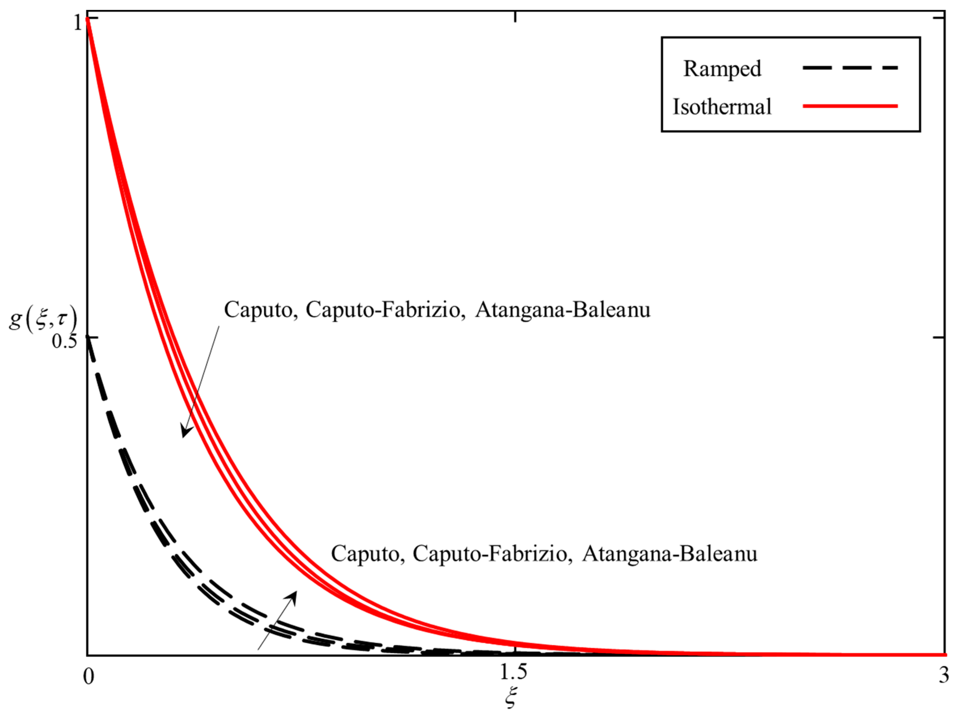
• For ramped temperature, the temperature field is higher for the ABC derivative followed by the CF and Caputo fractional derivatives, whereas, for isothermal temperature, the temperature field for the Caputo fractional derivative is higher than the CF and ABC, respectively.
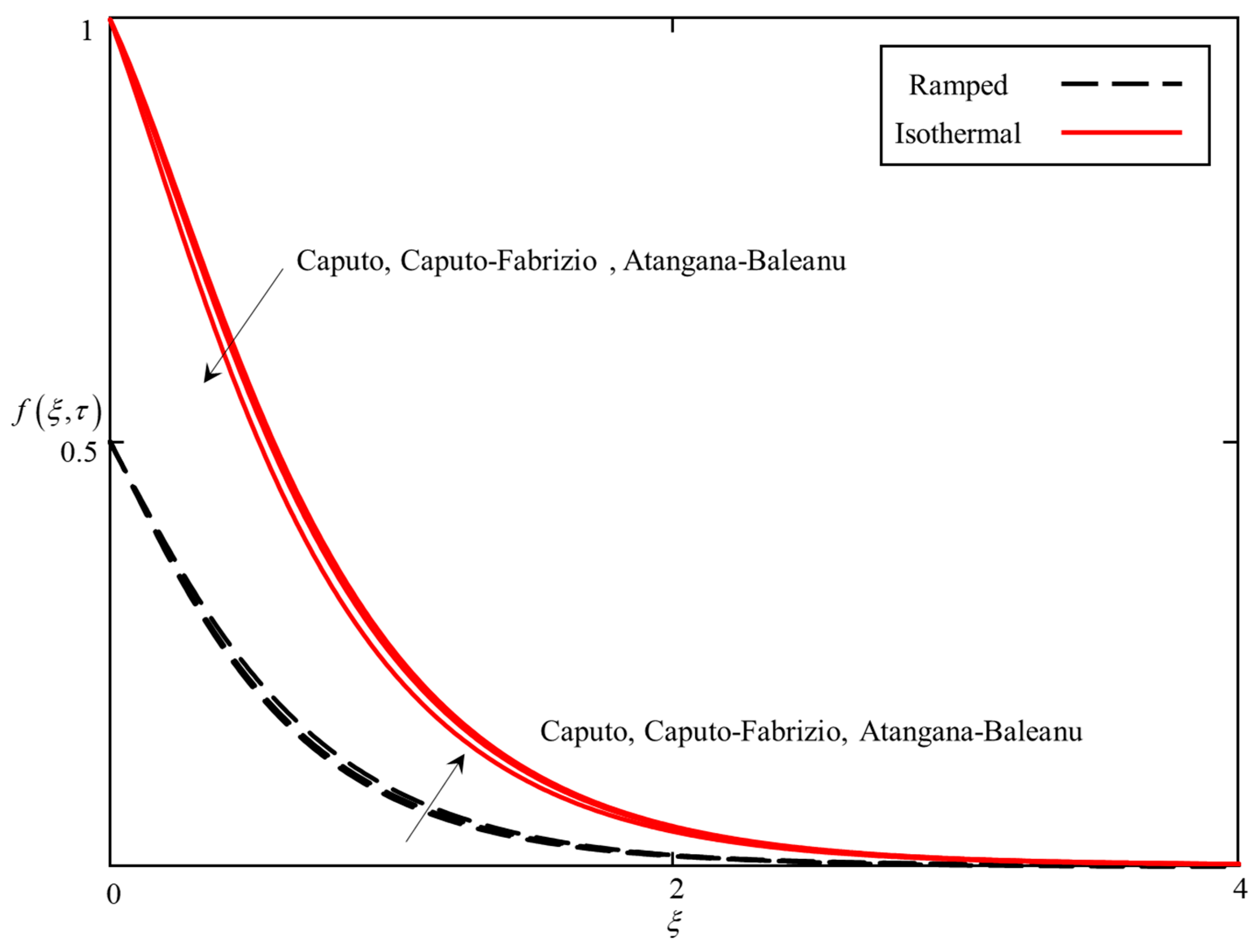
• The velocity field for the ABC derivative is higher than the CF and Caputo fractional derivatives in a ramped velocity case. However, this trend reverses in case of an isothermal velocity case.
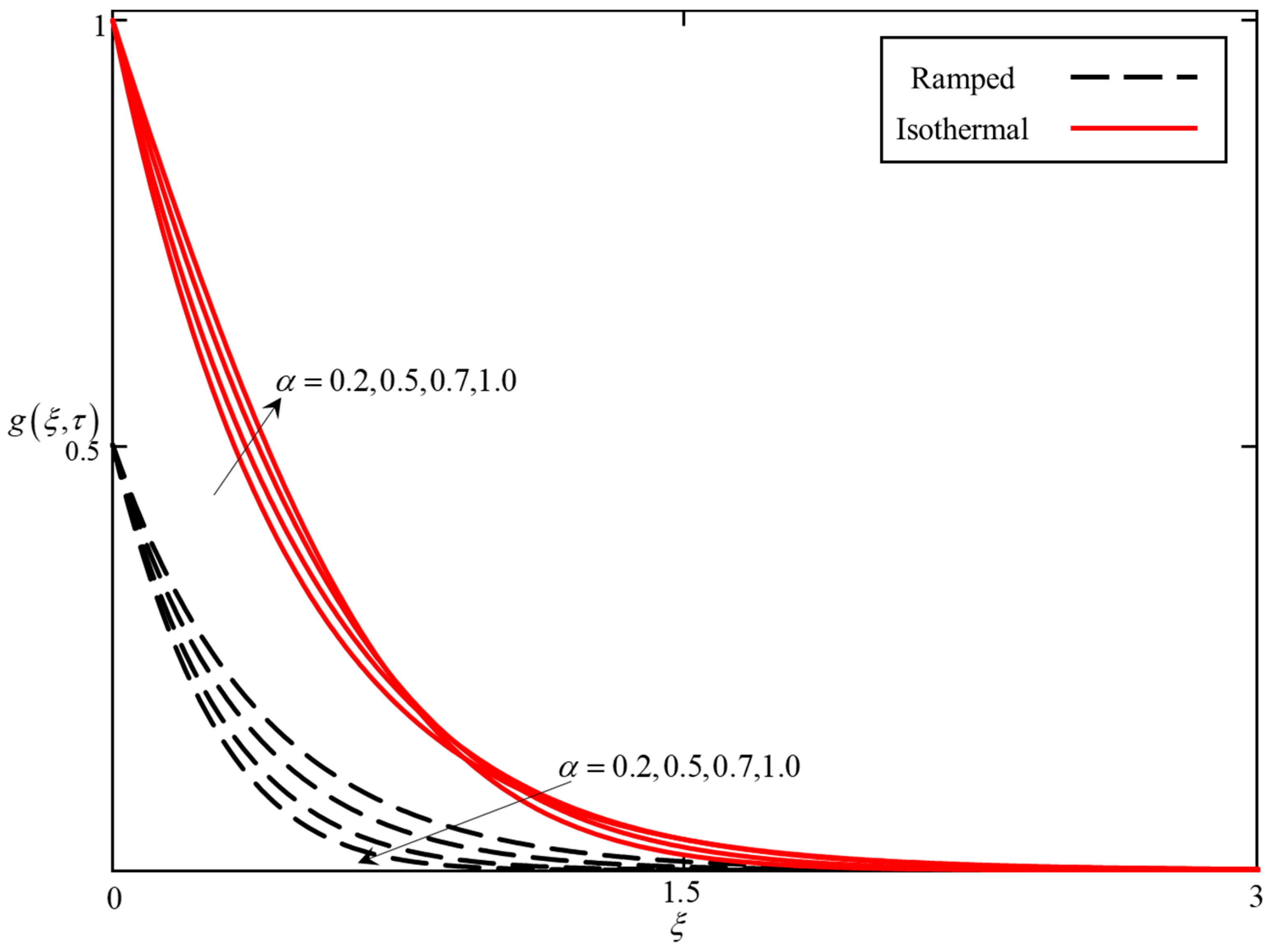
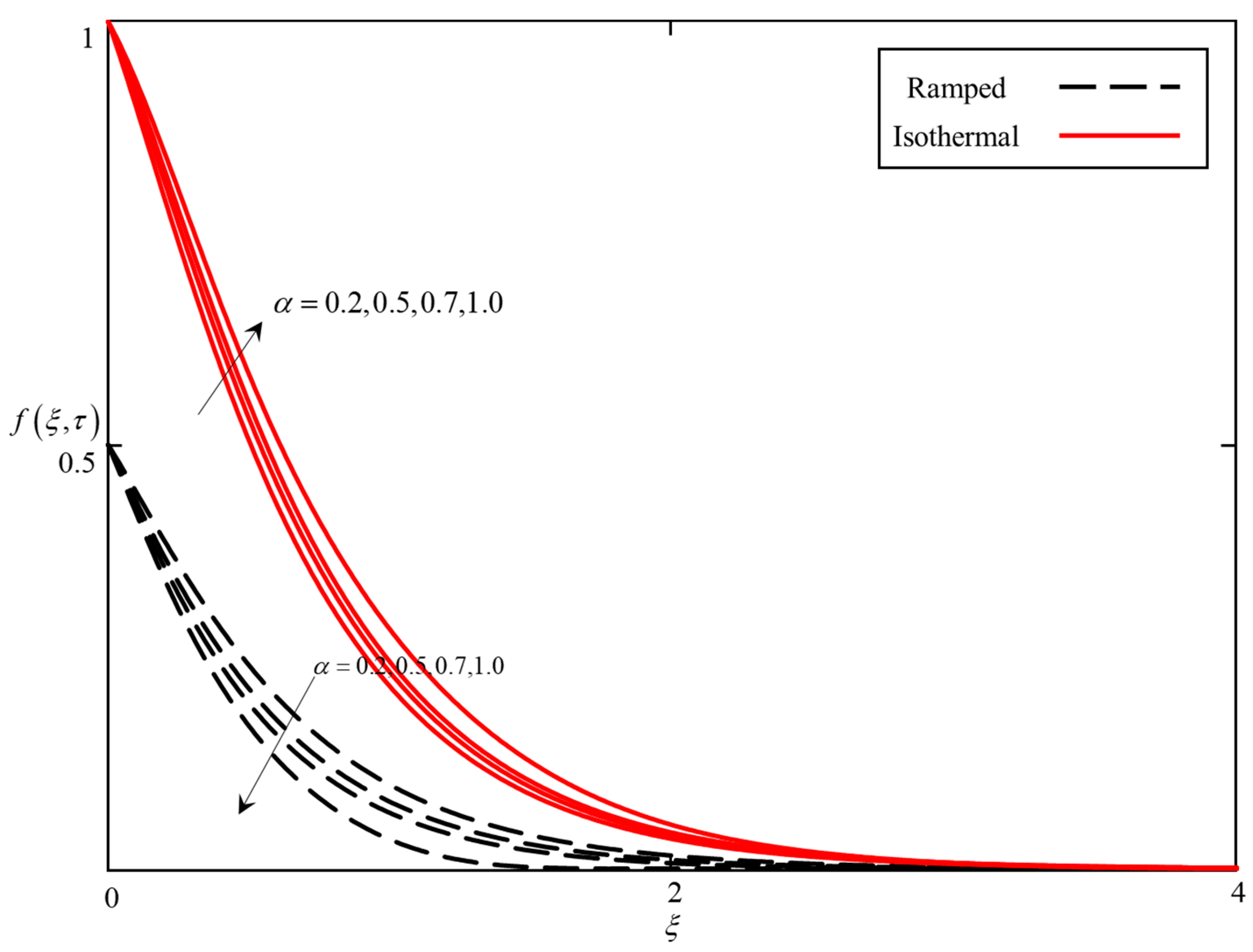
• An increase in α results in a reduction of the thickness of the temperature and velocity boundary layer. Consequently, a decrease in the temperature and velocity fields is observed.
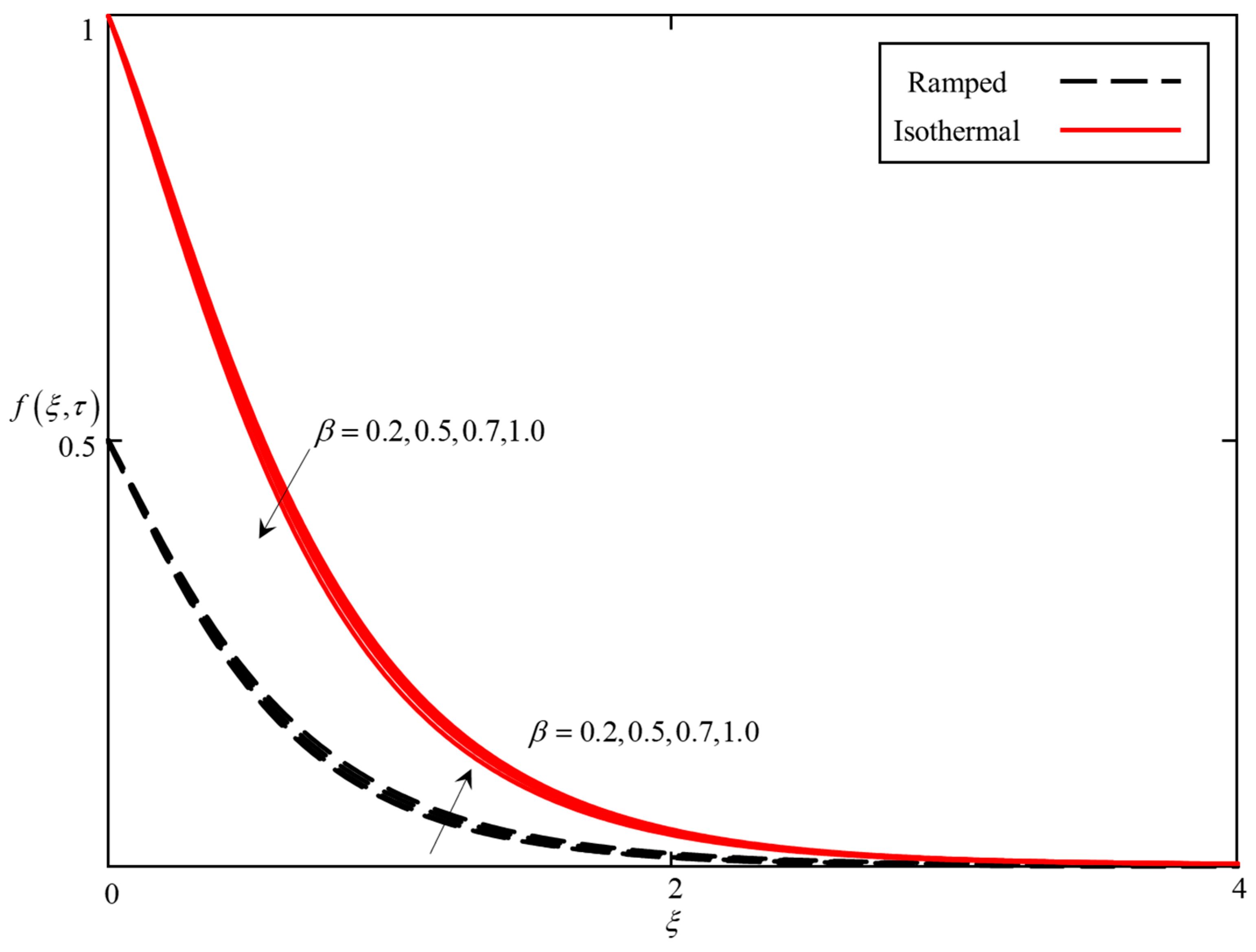
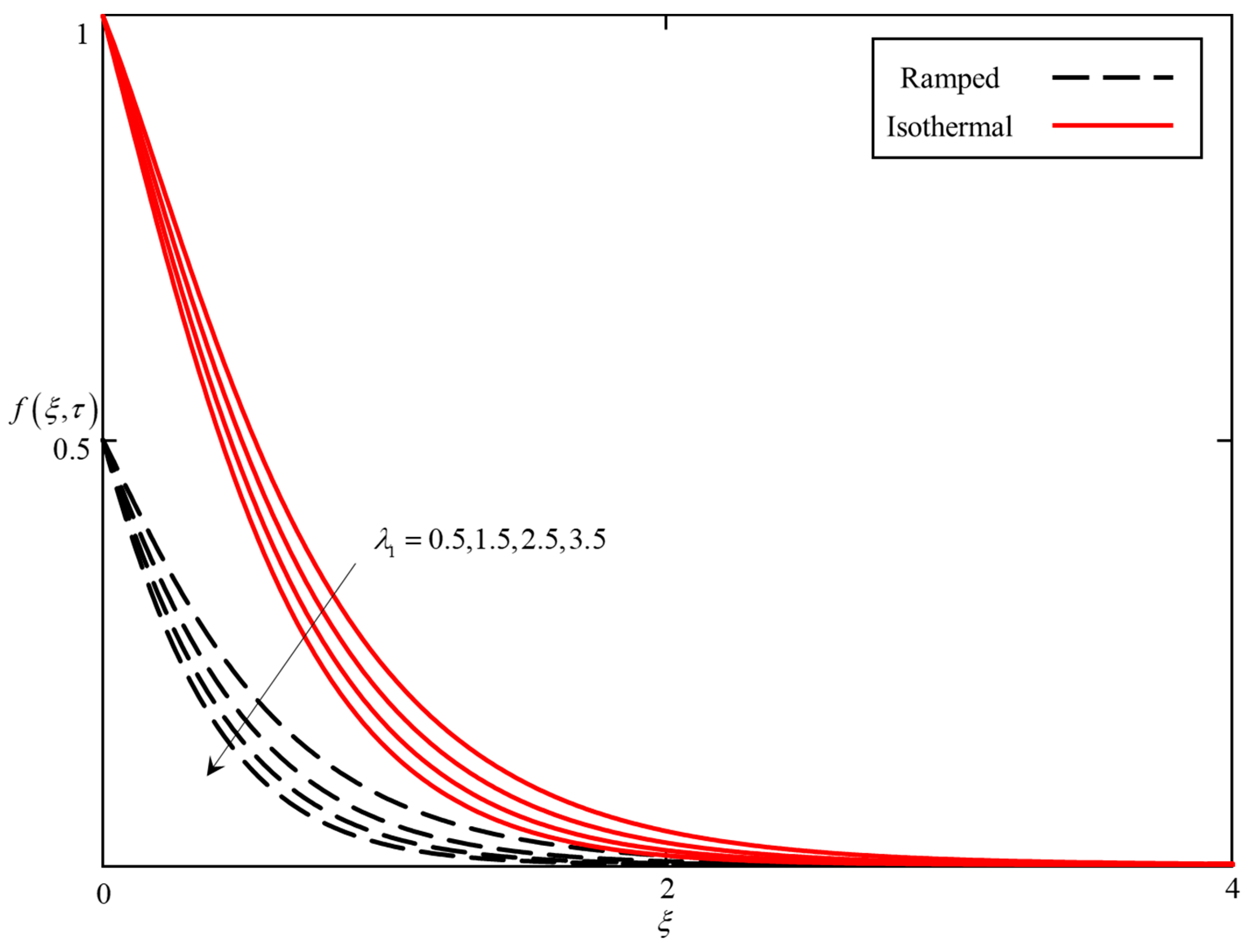
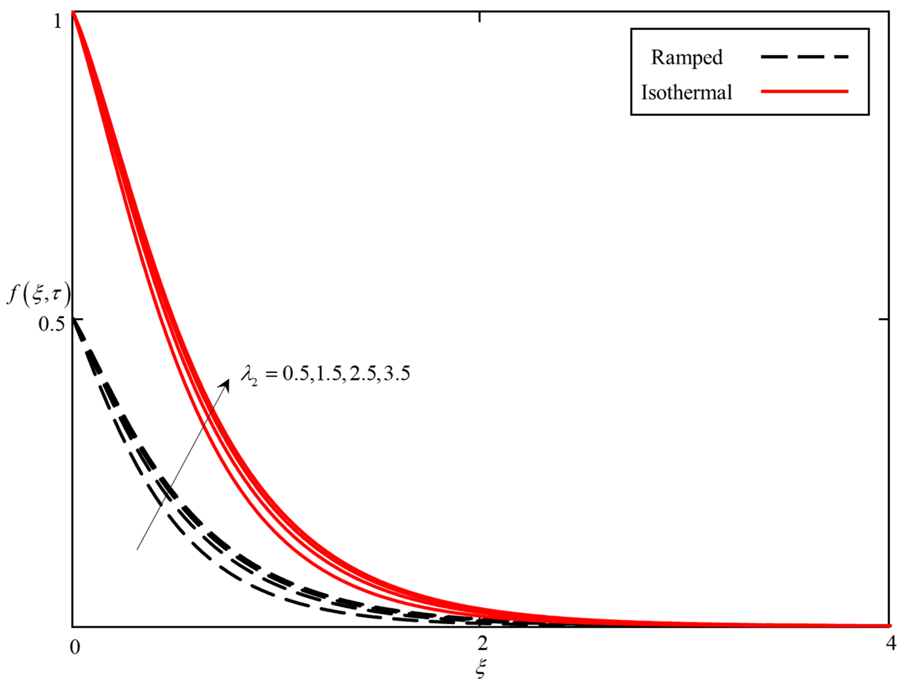
• It was found that the temperature field increases with increasing $\varphi$, and the velocity decreases with increasing $\varphi$.
• The effect of ${\lambda }_1$ and ${\lambda }_2$ on the velocity field is reversible.
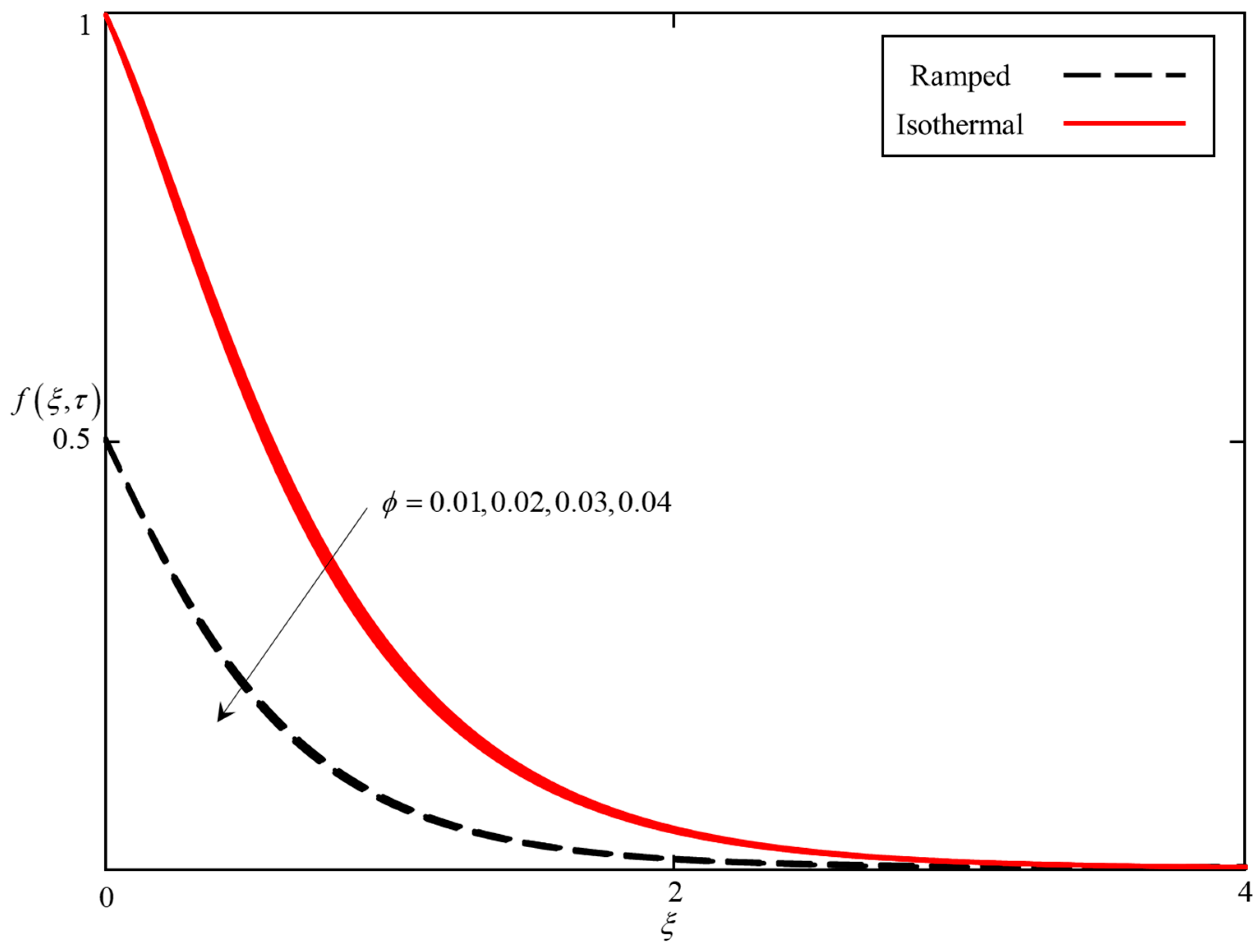
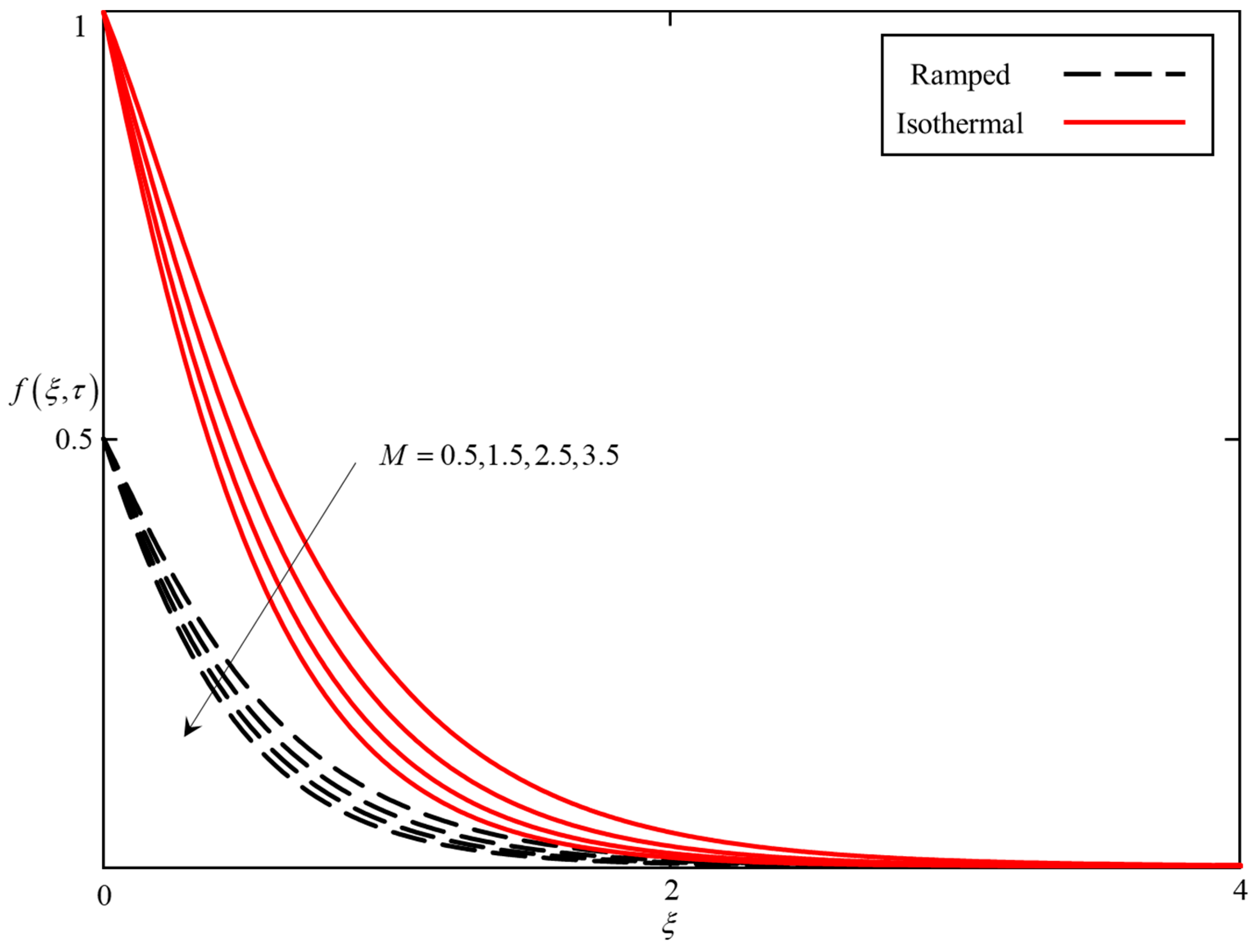
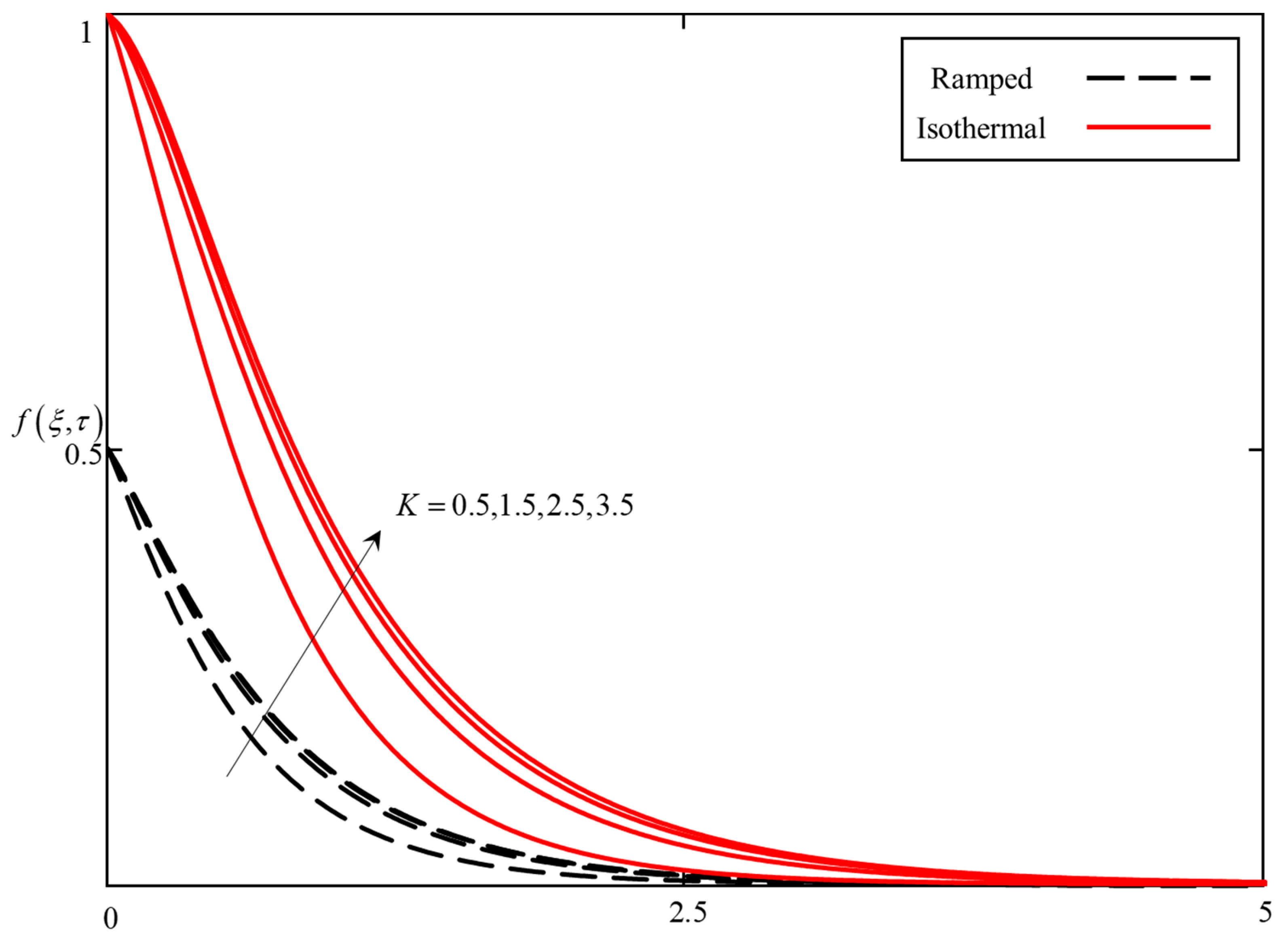
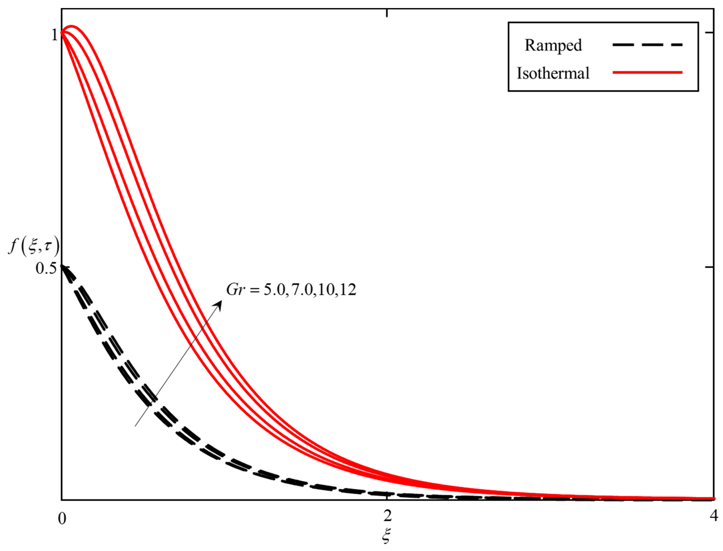
• An enhance in M leads to an enhancement in the Lorentz forces, which retarded the velocity, whereas increasing K and Gr increases the velocity field.

References

1. Franconi, C. Hyperthermia heating technology and devices. In Physics and Technology of Hyperthermia; Springer: Berlin/Heidelberg, Germany, 1987; pp. 80–122. [Google Scholar]
2. Saqib, M.; Khan, I.; Shafie, S. Generalized magnetic blood flow in a cylindrical tube with magnetite dusty particles. J. Magn. Magn. Mater. 2019, 484, 490–496. [Google Scholar] [CrossRef]
3. Ebaid, A.; Aljohani, A.F.; Aly, E.H. Homotopy perturbation method for peristaltic motion of gold-blood nanofluid with heat source. Int. J. Numer. Methods Heat Fluid Flow 2019, 30, 3121–3138. [Google Scholar] [CrossRef]
4. Lin, W.L.; Yen, J.Y.; Chen, Y.Y.; Jin, K.W.; Shieh, M.J. Relationship between acoustic aperture size and tumor conditions for external ultrasound hyperthermia. Med. Phys. 1999, 26, 818–824. [Google Scholar] [CrossRef] [PubMed]
5. Misra, J.; Shit, G. Biomagnetic viscoelastic fluid flow over a stretching sheet. Appl. Math. Comput. 2009, 210, 350–361. [Google Scholar] [CrossRef]
6. Choi, S.U.; Eastman, J.A. Enhancing Thermal Conductivity of Fluids with Nanoparticles; Argonne National Lab.: Lemont, IL, USA, 1995; pp. 99–105.
7. Shah, Z.; Islam, S.; Ayaz, H.; Khan, S. Radiative heat and mass transfer analysis of micropolar nanofluid flow of Casson fluid between two rotating parallel plates with effects of Hall current. J. Heat Transf. 2019, 141, 022401. [Google Scholar] [CrossRef]
8. Hsiao, K.-L. Micropolar nanofluid flow with MHD and viscous dissipation effects towards a stretching sheet with multimedia feature. Int. J. Heat Mass Transf. 2017, 112, 983–990. [Google Scholar] [CrossRef]
9. Lu, D.; Ramzan, M.; Ahmad, S.; Chung, J.D.; Farooq, U. A numerical treatment of MHD radiative flow of Micropolar nanofluid with homogeneous-heterogeneous reactions past a nonlinear stretched surface. Sci. Rep. 2018, 8, 1–17. [Google Scholar] [CrossRef] [PubMed] [Green Version]
10. Zubair, M.; Shah, Z.; Islam, S.; Khan, W.; Dawar, A. Study of Three dimensional Darcy–Forchheimer squeezing nanofluid flow with Cattaneo–Christov heat flux based on four different types of nanoparticles through entropy generation analysis. Adv. Mech. Eng. 2019, 11, 1687814019851308. [Google Scholar] [CrossRef] [Green Version]
11. Mebarek-Oudina, F.; Bessaïh, R. Numerical simulation of natural convection heat transfer of copper-water nanofluid in a vertical cylindrical annulus with heat sources. Thermophys. Aeromech. 2019, 26, 325–334. [Google Scholar] [CrossRef]
12. Hatami, M.; Hatami, J.; Ganji, D.D. Computer simulation of MHD blood conveying gold nanoparticles as a third grade non-Newtonian nanofluid in a hollow porous vessel. Comput. Methods Programs Biomed. 2014, 113, 632–641. [Google Scholar] [CrossRef]
13. Tzirtzilakis, E. A mathematical model for blood flow in magnetic field. Phys. Fluids 2005, 17, 077103. [Google Scholar] [CrossRef]
14. Papadopoulos, P.; Tzirtzilakis, E. Biomagnetic flow in a curved square duct under the influence of an applied magnetic field. Phys. Fluids 2004, 16, 2952–2962. [Google Scholar] [CrossRef] [Green Version]
15. Misra, J.; Ghosh, S. A mathematical model for the study of blood flow through a channel with permeable walls. Acta Mech. 1997, 122, 137–153. [Google Scholar] [CrossRef]
16. Misra, J.; Sinha, A.; Shit, G. A numerical model for the magnetohydrodynamic flow of blood in a porous channel. J. Mech. Med. Biol. 2011, 11, 547–562. [Google Scholar] [CrossRef]
17. Srinivas, S.; Vijayalakshmi, A.; Reddy, A.S. Flow and heat transfer of gold-blood nanofluid in a porous channel with moving/stationary walls. J. Mech. 2017, 33, 395–404. [Google Scholar] [CrossRef]
18. Caputo, M. Linear models of dissipation whose Q is almost frequency independent—II. Geophys. J. Int. 1967, 13, 529–539. [Google Scholar] [CrossRef]
19. Caputo, M.; Fabrizio, M. A new definition of fractional derivative without singular kernel. Progr. Fract. Differ. Appl. 2015, 1, 1–13. [Google Scholar]
20. Atangana, A.; Baleanu, D. New fractional derivatives with nonlocal and non-singular kernel: Theory and application to heat transfer model. Therm. Sci. 2016, 2016, 763–769. [Google Scholar] [CrossRef] [Green Version]
21. Khader, M.; Saad, K. A numerical approach for solving the fractional Fisher equation using Chebyshev spectral collocation method. Chaos Solitons Fractals 2018, 110, 169–177. [Google Scholar] [CrossRef]
22. Saad, K.; Khader, M.; Gómez-Aguilar, J.; Baleanu, D. Numerical solutions of the fractional Fisher’s type equations with Atangana-Baleanu fractional derivative by using spectral collocation methods. Chaos Interdiscip. J. Nonlinear Sci. 2019, 29, 023116. [Google Scholar] [CrossRef]
23. Jan, R.; Khan, M.A.; Kumam, P.; Thounthong, P. Modeling the transmission of dengue infection through fractional derivatives. Chaos Solitons Fractals 2019, 127, 189–216. [Google Scholar] [CrossRef]
24. Gómez-Aguilar, J.; Atangana, A. New insight in fractional differentiation: Power, exponential decay and Mittag-Leffler laws and applications. Eur. Phys. J. Plus 2017, 132, 13. [Google Scholar] [CrossRef]
25. Atangana, A.; Gómez-Aguilar, J. A new derivative with normal distribution kernel: Theory, methods and applications. Phys. A Stat. Mech. Its Appl. 2017, 476, 1–14. [Google Scholar] [CrossRef]
26. Ali, F.; Saqib, M.; Khan, I.; Sheikh, N.A. Application of Caputo-Fabrizio derivatives to MHD free convection flow of generalized Walters’-B fluid model. Eur. Phys. J. Plus 2016, 131, 377. [Google Scholar] [CrossRef]
27. Fetecau, C.; Fetecau, C. The first problem of Stokes for an Oldroyd-B fluid. Int. J. Non-Linear Mech. 2003, 38, 1539–1544. [Google Scholar] [CrossRef]
28. Saqib, M.; Khan, I.; Shafie, S.; Qushairi, A. Recent Advancement in Thermophysical Properties of Nanofluid and Hybrid Nanofluid: An Overview. City Univ. Int. J. Comput. Anal. 2019, 3, 16–25. [Google Scholar]
29. Fetecau, C.; Fetecau, C.; Khan, M.; Vieru, D. Decay of a potential vortex in a generalized Oldroyd-B fluid. Appl. Math. Comput. 2008, 205, 497–506. [Google Scholar] [CrossRef]
30. Tiwana, M.H.; Mann, A.B.; Rizwan, M.; Maqbool, K.; Javeed, S.; Raza, S.; Khan, M.S. Unsteady Magnetohydrodynamic Convective Fluid Flow of Oldroyd-B Model Considering Ramped Wall Temperature and Ramped Wall Velocity. Mathematics 2019, 7, 676. [Google Scholar] [CrossRef] [Green Version]
31. Khalid, A.; Khan, I.; Khan, A.; Shafie, S.; Tlili, I. Case study of MHD blood flow in a porous medium with CNTS and thermal analysis. Case Stud. Therm. Eng. 2018, 12, 374–380. [Google Scholar] [CrossRef]
32. Koriko, O.K.; Animasaun, I.; Mahanthesh, B.; Saleem, S.; Sarojamma, G.; Sivaraj, R. Heat transfer in the flow of blood-gold Carreau nanofluid induced by partial slip and buoyancy. Heat Transf.—Asian Res. 2018, 47, 806–823. [Google Scholar] [CrossRef]
33. Aman, S.; Khan, I.; Ismail, Z.; Salleh, M.Z. Impacts of gold nanoparticles on MHD mixed convection Poiseuille flow of nanofluid passing through a porous medium in the presence of thermal radiation, thermal diffusion and chemical reaction. Neural Comput. Appl. 2018, 30, 789–797. [Google Scholar] [CrossRef] [PubMed] [Green Version]
34. Podlubny, I. Fractional Differential Equations: An Introduction to Fractional Derivatives, Fractional Differential Equations, to Methods of Their Solution and Some of Their Applications; Elsevier: Amsterdam, The Netherlands, 1998. [Google Scholar]
35. Khan, I.; Saqib, M.; Ali, F. Application of time-fractional derivatives with non-singular kernel to the generalized convective flow of Casson fluid in a microchannel with constant walls temperature. Eur. Phys. J. Spec. Top. 2017, 226, 3791–3802. [Google Scholar] [CrossRef]
36. Khan, I.; Saqib, M.; Ali, F. Application of the modern trend of fractional differentiation to the MHD flow of a generalized Casson fluid in a microchannel: Modelling and solution⋆. Eur. Phys. J. Plus 2018, 133, 262. [Google Scholar] [CrossRef]
Figure 1. Physical sketch and coordinate system.
Applsci 10 03886 g001
Figure 2. Solution methodology and operational framework.
Applsci 10 03886 g002
Figure 3. Comparison of the temperature field for Caputo, Caputo–Fabrizio, and Atangana–Baleanu fractional derivatives, when α = 0.5 , ϕ = 0.04 , Pr = 21 .
Applsci 10 03886 g003
Figure 4. Comparison of the velocity field for Caputo, Caputo–Fabrizio and Atangana–Baleanu fractional derivatives, when α = 0.5 , β = 0.5 ϕ = 0.04 , λ 1 = 0.5 , λ 2 = 0.5 , M = 0.5 , K = 0.5 Pr = 21 , and G r = 5.0 .
Applsci 10 03886 g004
Figure 5. Consequence of α on the temperature field, when ϕ = 0.04 and Pr = 21 .
Applsci 10 03886 g005
Figure 6. Consequence of α on the velocity field, when β = 0.5 , ϕ = 0.04 , λ 1 = 0.5 , λ 2 = 0.5 , M = 0.5 , K = 0.5 Pr = 21 , and G r = 5.0 .
Applsci 10 03886 g006
Figure 7. Consequence of β on the velocity field, when α = 0.5 , ϕ = 0.04 , λ 1 = 0.5 , λ 2 = 0.5 , M = 0.5 , K = 0.5 Pr = 21 , and G r = 5.0 .
Applsci 10 03886 g007
Figure 8. Consequence of ϕ on the temperature field when α = 0.5 and Pr = 21
Applsci 10 03886 g008
Figure 9. Consequence of ϕ on the velocity field, when α = 0.5 , β = 0.04 , λ 1 = 0.5 , λ 2 = 0.5 , M = 0.5 , K = 0.5 Pr = 21 , and G r = 5.0 .
Applsci 10 03886 g009
Figure 10. Consequence of λ 1 on the velocity field, when α = 0.5 , β = 0.5 , ϕ = 0.04 , λ 2 = 0.5 , M = 0.5 , K = 0.5 Pr = 21 , and G r = 5.0 .
Applsci 10 03886 g010
Figure 11. Consequence of λ 2 on the velocity field, when α = 0.5 , β = 0.5 , ϕ = 0.04 , λ = 0.5 , M = 0.5 , K = 0.5 , Pr = 21 , and G r = 5.0 .
Applsci 10 03886 g011
Figure 12. Consequence of M on the velocity field, when α = 0.5 , β = 0.5 , ϕ = 0.04 , λ 1 = 0.5 , λ 2 = 0.5 , K = 0.5 , Pr = 21 , and G r = 5.0 .
Applsci 10 03886 g012
Figure 13. Consequence of K on the velocity field, when α = 0.5 , β = 0.5 , ϕ = 0.04 , λ 1 = 0.5 , λ 2 = 0.5 , M = 0.5 , Pr = 21 , and G r = 5.0 .
Applsci 10 03886 g013
Figure 14. Consequence of Gr on the velocity field, when α = 0.5 , β = 0.5 , ϕ = 0.04 , λ 1 = 0.5 , λ 2 = 0.5 , M = 0.5 , K = 0.5 , and Pr = 21 .
Applsci 10 03886 g014