Basic Analysis of Uncertainty Sources in the CFD Simulation of a Shell-and-Tube Latent Thermal Energy Storage Unit

Abstract

Computational Fluid Dynamics (CFD) simulations are increasingly employed in the development of latent thermal energy storage units. Yet there are often strong deviations between the experiments and numerical results. To unveil the sources of the deviations for the CFD simulation of a vertical shell-and-tube latent thermal energy storage unit, a basic analysis of different uncertainties is undertaken in this paper. Consequently, the effect of a variation of 10 material properties, six initial and boundary conditions, as well as a displacement of the temperature measuring points in the simulation, are examined. The results depict that the influence of the substance data depend on the output variable under consideration. Beside material properties, which have almost no influence, there are some properties that influence the power and the global liquid phase fraction over time, and a third group, which also has an influence on the mean power. Partly in contrast to results found in literature, the highest influence on the mean power occurs for the heat losses (which are varied in an on/off manner), the density, and the melting enthalpy (both varied by $\pm 10\%$).

1. Introduction

The increasing share of renewable energies raises the temporal mismatch between energy production and consumption. As a consequence, energy storage systems attract more and more attention due to their ability to store and deliver energy when it is needed. Thermal energy storage systems are a cost effective option, not only for storing thermal energy, but they are also promising for demand side management, as well as for pumped thermal electricity storage [1]. If thermal energy needs to be stored in a narrow temperature range, or the energy storage density is of major importance, latent thermal energy storage systems (LTESS) are the right choice [2]. The high storage density of these storage units is a result of exploiting the latent heat of a phase change. Usually, solid/liquid phase changes of the so-called phase change materials (PCM) are chosen for this purpose. Analyzing, designing, and optimizing LTESS is more and more supported by numerical simulations. Thus far, however, major uncertainties have existed in these simulations, mainly due to a large variety of material properties reported in the literature [3], guessed constants in the numerical models, and a lack of highly precise validation experiments for most applications. In addition, it seems that these uncertainties are often not disclosed, but rather that efforts are being made to hide them by adjusting the constants and selecting the best fitting substance data found in literature.

Compared to the vast amount of publications dealing with the numerical simulation of PCM [4], only a very limited number of papers deal with analyzing the above described uncertainties. To model a solid-liquid phase change problem on a fixed grid, including natural convection in the liquid phase, a switch-off technique has to be implemented in the model to cancel the velocity in the solid phase. Voller et al. [5] studied, on a very coarse grid, three methods, (i) an approach which explicitly overwrites the velocity at a certain amount of solid phase in a control volume [6]; (ii) the variable viscosity method (VVM) that allocates a very high viscosity to the solid phase [7]; and (iii) the porosity approach, which describes the switch-off with the help of a porosity function. The porosity approach was found to be the most promising one and is—with a different formulation [8]—still the most used approach nowadays followed by the VVM. Both methods rely on arbitrary constants to describe the porosity or the viscosity in the solid phase. Voller et al. [5] concluded that a very high Darcy constant is like a switch-off as soon as the liquid fraction becomes smaller than 1 in the considered control volume. In Brent et al. [8], it is also stated that for a pure material the porosity has no real physical meaning, but should only ramp down the velocity. Unfortunately, most PCM are not pure materials and, in consequence, the lack of a clear procedure to determine the Darcy constant for the porosity approach and the solid viscosity for the VVM has led to a practice of fitting the constants to the experimental results. This procedure, however, is polluted by the uncertainties within the numerical model, the material properties, and the experiment. In addition, the “right” value of the constants might be influenced by the boundary conditions, the mesh, etc., and is, therefore, not transferable. The effect of different values of the Darcy constant and the solid viscosity was analyzed by Kheirabadi and Groulx [9], and several other authors analyzed the effect of different Darcy constants [10,11,12,13,14]. Generally, the results indicate that a higher Darcy constant, as well as a higher solid viscosity, slow down the phase change process, but a too high constant may lead to an unphysical behavior and even increase the phase change rate [13]. Furthermore, the results show (i) that the influence of the Darcy constant in the porosity approach seems to be higher than the influence of the constants in a combined VVM porosity approach [9]; (ii) that the influence of the Darcy constant is higher for melting than for solidification [12]; and (iii) that the influence of the Darcy constant depends on the orientation of the PCM container [11] and is less important when heat conduction dominates [10,11,12]. In addition, Voller and Prakash [15] have shown that not only the absolute value but also the shape of the Darcy term function influences the phase change behavior. Recently, Ebrahimi et al. [14] have stated that the influence of the Darcy constant reduces for finer meshes and for an isothermal phase change.

Beside the switch-off techniques, the fixed grid methods depend on a method that takes into account the latent heat. Overviews of these so-called enthalpy methods can be found in literature [16,17,18]. König-Haagen et al. [19] analyzed five common enthalpy methods and concluded that for a broad range of parameters, four of the five tested methods gave almost identical results, only the applied apparent heat capacity method performed poorly. In addition, the effect of two different formulations of the convective term in the energy equation was studied. It was found that a formulation that only convects sensible enthalpy is more resilient compared to a formulation were all enthalpy is convected. For cement mortar with PCM, a purely conductive analysis was performed by Tittelein et al. [20]. Three methods were tested and the best results were achieved with an enthalpy method that models the cement mortar PCM composite as a binary mixture. The tested apparent heat capacity method gave unphysical results. Other examples of tested numerical setups and settings are the tolerance for solving the energy equation [21] and different discretization schemes for the convective term of the energy equation [22]. In general, both the tolerance within the energy equation and the discretization of the convective term show a large impact; however, for the tolerance, it was not observed for all solvers tested. Moreover, Shmueli et al. [13] compared the Semi-Implicit Method for Pressure Linked Equations (SIMPLE) with the Pressure-Implicit with Splitting of Operators (PISO) scheme for solving the Navier–Stokes equation and the PREssure STaggering Option (PRESTO!) with the body-force-weighted approach for interpolating the pressure. There were no differences found in the results achieved with the SIMPLE or the PISO scheme, but the PRESTO! approach showed a better agreement with the experiments than the body-force-weighted approach. Lastly, it should be noted that independency studies for the mesh and the time step are commonly reported within papers on LTESS simulation, and a few authors compare two-dimensional (2D) with three-dimensional (3D) simulations showing that distinctive differences in the flow patterns may appear between both approaches [22,23].

Analyses regarding the material properties mostly only focused on one or a few specific aspects. From analyses with simple analytical models, Günter et al. [24] drew some basic conclusions regarding the effects of uncertain material data. The effect of differential scanning calorimetry (DSC) results that were achieved with different heating rates were investigated numerically [25,26], and the influence of the width of the melting range on the numerical results was studied by several authors [9,10,15,21,27,28]. Interestingly, it is reported that a larger melting range may either lead to a faster phase change [9,21] or a slower one [9]. Galione et al. [22] compared simulation results achieved with temperature dependent material properties to results that were obtained with constant material properties. It seemed that next to the density change between solid and liquid octadecane, the variation of the thermal conductivity of the liquid PCM has the largest influence on the melting rate. Soni et al. [29] checked the impact of assuming identical material properties in the solid and the liquid state compared to differing values for some of the material properties. The authors claim that the model with different material properties in the solid and liquid phase has better potential to reduce the discrepancy between simulation and experiment than the model with constant material properties. The effect of the uncertainty of the material properties data was analyzed in detail with purely diffusive phase change models by Dolado et al. [27], Zsembinszki et al. [30], and Mazo et al. [28]. In all three studies, the melting temperature is the most important, or one of the most important, material properties. Interestingly, the detailed uncertainty analyses performed in Dolado et al. [27] and Mazo et al. [28] allow to propose a certain set of allowed uncertainties in the material properties to achieve a predefined maximum error in the numerical results. Possible variances in the start and boundary conditions, as well as in the geometric data, are investigated by Dolado et al. [27] and Zsembinszki et al. [30]. Combined with the detailed analyses for the material properties, this allows for a fair comparison of the numerical results with experimental results as the overlap of both results can be taken as a measure for the agreement.

In summary, there are still large uncertainties present when it comes to the simulation of an LTESS, and even a basic validation of models for melting processes is still subject to distinct uncertainties. On the other hand, it is common practice to fit model constants, such as the Darcy constant to experimental results, and/or to choose material properties that fit the experimental results best. However, errors due to uncertain material properties, too coarse meshes and incorrect model assumptions as well as uncertainties in the experiment may have been hidden by a new error, which gives the illusion of a highly precise simulation. As stated above, there are already several studies on the influence of different enthalpy methods or switch-off techniques. However, to the authors’ knowledge, there is no Computational Fluid Dynamics (CFD) study on LTESS so far that takes into account the uncertainties of the material properties, of the initial and boundary conditions, as well as of the experiment. Therefore, the aim of this work is to investigate these uncertainties with a basic sensitivity analysis performed with a CFD model describing an experiment from literature [31].

2. Materials and Methods

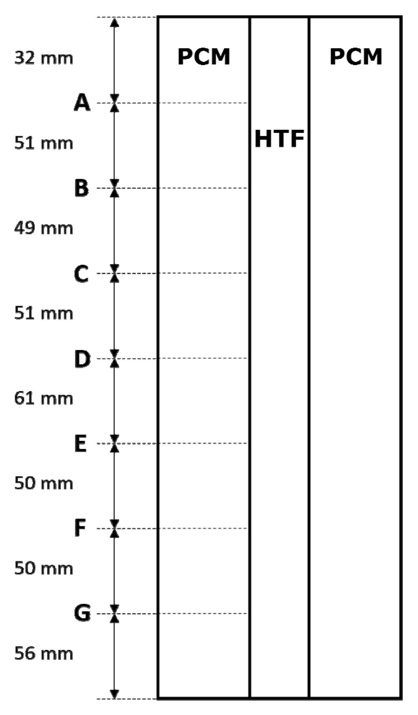
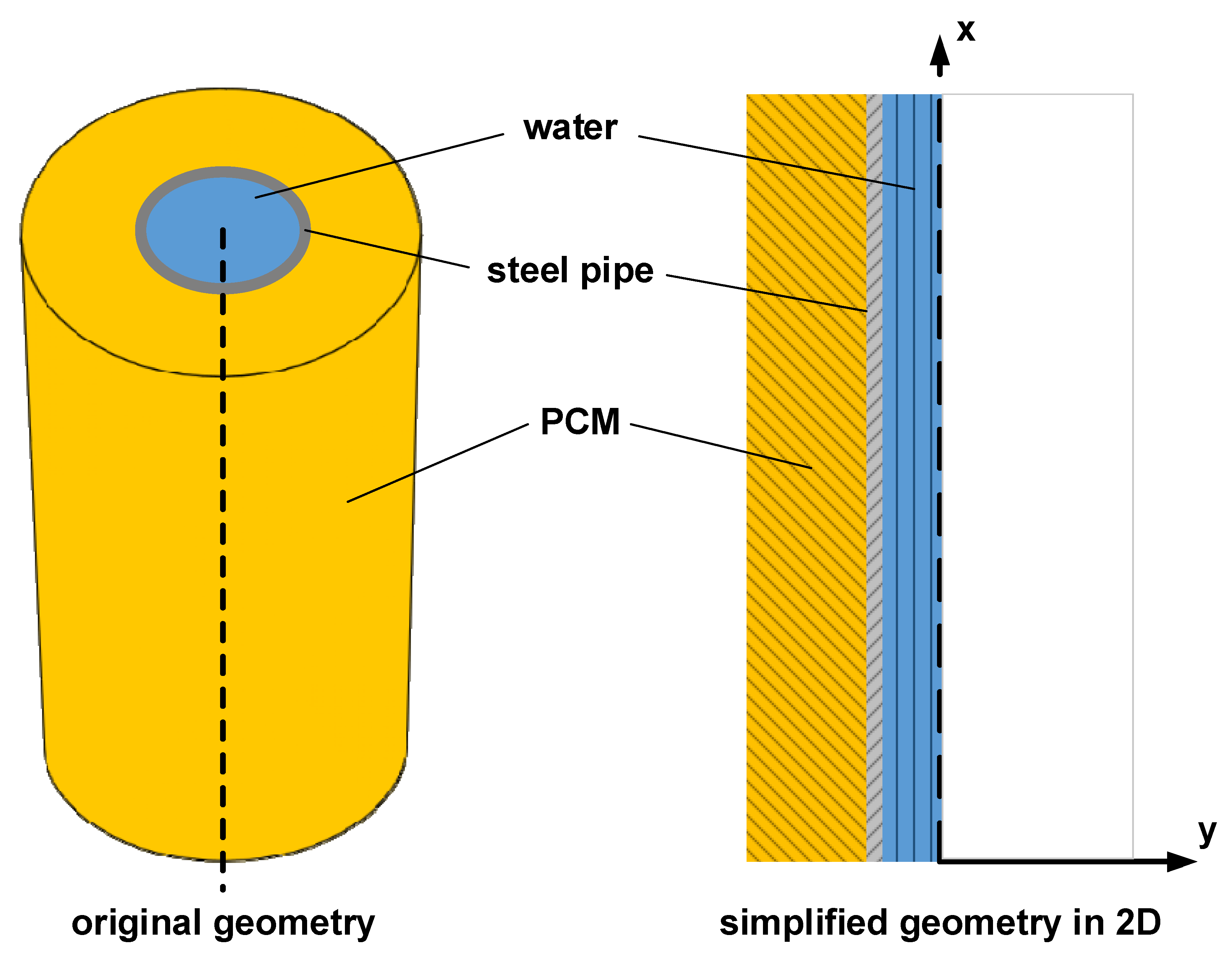
2.1. Set-Up

A vertical shell-and-tube type latent thermal energy storage unit is used as the set-up. The storage unit consists of two pipes. The outer pipe is made of Plexiglas and has an inner and an outer diameter of 44 mm and 50 mm, respectively. The inner and outer diameter of the inner pipe (made of stainless steel) are 10 mm and 15 mm, respectively. The height of the storage unit is 400 mm and a detailed description of the storage system is given in Longeon et al. [31]. A basic scheme of the storage system and the vertical layers in which thermocouples are placed in the PCM within the experiment can be found in Figure 1. A selection of the thermocouples used in the experiment is considered for comparison with the numerical model (see

Table 1. Measurement point positions.

Measuring Point Identifiers	Radius in mm	Height in mm
B-b	16	317
D-a	13	217
D-b	16	217
D-c	19	217
F-b	16	106

). The uppercase letter of the identifier refers to the vertical layer and the lowercase letter stands for the horizontal position.

For the heat transfer fluid (HTF) water and the steel pipe, the material properties available in ANSYS Fluent are used. The heat conductivity of the Plexiglas is set to ${\lambda }_{Plexi}=0.19\frac{\mathrm{W}}{\mathrm{mK}}$ and the material properties of the PCM RT 35—nowadays called RT 35 HC—(Rubitherm Technologies GmbH, Berlin, Germany) can be found in

Table 2. Material properties of RT 35—nowadays called RT 35 HC.

Physical Properties	Value	Unit	Source
$\rho$	760	$\frac{\mathrm{kg}}{{\mathrm{m}}^3}$	[31]
$c_s$	5.0	$\frac{\mathrm{kJ}}{\mathrm{kg}·\mathrm{K}}$	[32]
$c_l$	2.1	$\frac{\mathrm{kJ}}{\mathrm{kg}·\mathrm{K}}$	[32]
$\lambda$	0.2	$\frac{\mathrm{W}}{\mathrm{m}·\mathrm{K}}$	[31]
$L$	220	$\frac{\mathrm{kJ}}{\mathrm{kg}}$	[32]
$T_s$	34.5	$°\mathrm{C}$	[32]
$T_l$	36.0	$°\mathrm{C}$	[32]
$\eta$	see Equation (1)	$\mathrm{Pa}\times \mathrm{s}$	own measurements
$\beta$	0.001	$\frac{1}{\mathrm{K}}$	[31]

.

The viscosity was measured with the IMETER Mess System and approximated by a linear fit.

$$\eta /\mathrm{Pa}\times \mathrm{s}=8.33075\times -1.09187\times {10}^{-4}·T/℃.$$

(1)

For $c_s$ a high value appears because already below $T_s$ increased values for the heat capacity occur. The value of 5 $\frac{\mathrm{kJ}}{\mathrm{kg}·\mathrm{K}}$ was measured at 30 °C by Rösler [32].

2.2. Boundary and Initial Conditions

At the beginning of every charging and discharging process, the storage system has a uniform temperature. The storage system is charged from the top and discharged from the bottom. After charging and discharging, the phase change process has already been finished in the reference simulation. The initial and boundary conditions of the reference simulation can be seen in

Table 3. Initial and boundary conditions for the reference simulation.

Variable	Value	Unit
$T_{init,char}$	23.79	$℃$
$T_{init,dis}$	47.15	$℃$
$T_{in,char}$	53.17	$℃$
$T_{in,dis}$	18.51	$℃$
$t_{char}$	8000	$\mathrm{s}$
$t_{dis}$	10,000	$\mathrm{s}$
$u_{in}$	$10\times {10}^{-3}$	$\frac{\mathrm{m}}{\mathrm{s}}$
${\dot{Q}}_{loss}$	0	$\mathrm{W}$

.

According to the publication of Longenon et al. [31], it is assumed in the reference case that the outer wall is adiabatic. Throughout the variations, $t_{char}$ as well as $t_{dis}$ are kept constant, and $T_{start}$, $T_{in}$ and $u_{in}$ are varied by a fixed value. Additionally, $T_{in}$ is integrated once as a time curve, for $u_{in}$ a parabolic velocity profile is implemented once at the inlet and the heat losses are considered once. The time curves for $T_{in}$ are fitted to the measured inlet temperatures leading to

$$T_{in}\left(t\right)/°\mathrm{C}=326.3\times e^{t\times 1.909\times {10}^{-7}\times 1/\mathrm{s}}-1.162\times e^{-t\times 1.419\times {10}^{-3}\times 1/\mathrm{s}}$$

(2)

for charging and

$$T_{in}\left(t\right)/°\mathrm{C}=291.05+2.314\times \left(1-e^{-t/443.7\times 1/\mathrm{s}}\right)-1.805\times \left(1-e^{-t/1326\times 1/\mathrm{s}}\right)$$

(3)

for discharging. This results in maximum inlet temperature variations of about 1.7 K and 1.1 K for charging and discharging, respectively. To estimate the influence of the heat losses, a heat loss coefficient is defined, which includes the thermal resistance of the Plexiglas wall and the natural convection at the outside.

$$U_{loss}={\left(R_{Plexi}A+\frac{1}{{\alpha }_{ext}}\right)}^{-1}$$

(4)

The natural convection at the outer surface $A$ is calculated by means of laminar natural convection for a vertical cylinder [33]. Assuming $T_{W,i}=\left(T_s+T_l\right)/2=35.25℃$ on average and $T_{amb}=18.5℃$ one gets for the overall heat flux coefficient $U_{loss}=3.87\frac{\mathrm{W}}{{\mathrm{m}}^2\mathrm{K}}$.

2.3. Numerical Model

The numerical model was set up in ANSYS Fluent 15.0 (ANSYS, Inc., Canonsburg, PA, US). The simulation domain consists of three different areas—the HTF in the inner pipe, the wall of the inner pipe, and the PCM in the annular gap. Within the HTF and the PCM, a laminar flow is assumed and the density is set constant and the Boussinesq approximation is used for the PCM. An enthalpy porosity method is applied [8] for the PCM, which implies two source terms. One in the energy equation to account for the latent enthalpy and another one, a Darcy-type source term, in the momentum equation to switch off the velocity in the solid region. The continuity equation with constant density is:

$$\nabla \times u=0$$

(5)

and the momentum equation of the PCM becomes

$$\rho \left[\frac{\partial \mathbf{u}}{\partial \mathrm{t}}+\nabla \times \left(\mathbf{uu}\right)\right]=\nabla \times \tau -\nabla \mathrm{p}+D\mathbf{u}+\rho \mathbf{g}$$

(6)

where the Boussinesq approximation is implemented by

$$\rho \mathbf{g}={\rho }_0\mathbf{g}\left[1-\beta \left(T-T_0\right)\right]$$

(7)

and the Darcy term is written as

$$D=-C_{\mathrm{I}}\frac{{\left(1-{\alpha }_F\right)}^2}{{\alpha }_F^3+C_{\mathrm{I}\mathrm{I}}}.$$

(8)

The energy equation of the PCM is

$$\rho c\left[\frac{\partial T}{\partial t}+\nabla \times \left(\mathit{u}T\right)\right]=\nabla \times \left(\lambda \nabla T\right)-\rho L\left(\frac{\partial {\alpha }_F}{\partial t}+\mathit{u}\nabla {\alpha }_F\right).$$

(9)

In Equations (8) and (9) ${\alpha }_F$ describes the liquid fraction, which is defined as

$${\alpha }_F=\frac{h-h_s}{h_l-h_s}$$

(10)

and limited to values from 0 to 1. The update technique is described in detail in literature [34].

2.4. Mesh and Solver

The simulation domain was simplified. Only two dimensions are considered and an axis symmetry was used (see Figure 2). The mesh is orthogonal, has a maximum growth rate of 1.2 in y-direction in the HTF domain and cells with constant size in the domains of the pipe wall and the PCM. Since the mesh consists of 100 cells in x-direction and 122 cells in y-direction, it is ensured that a much finer resolution is generated in the expected direction of the largest gradients of velocity, temperature, enthalpy, etc. All relevant solver settings of the final simulations can be found in

Table A1. Final solver settings.

Subfield	Parameter	Value
solution method	pressure-velocity coupling	PISO extrapolated
	discretization (pressure)	PRESTO!
	discretization (momentum)	QUICK
	discretization (energy)	QUICK
	discretization (time)	first order implicit
residuals	continuity	${10}^{-6}$
	x-velocity	${10}^{-6}$
	y-velocity	${10}^{-6}$
	energy	${10}^{-10}$
simulation parameter	time step	0.2 s
	$C_{\mathrm{I}\mathrm{I}}$	0.001

in the Appendix A.

The mesh, the pressure-velocity coupling, the discretization of the convective terms in the energy, and momentum equation, as well as the time step will be analyzed in Section 3.1. Higher order methods for time discretization showed an unstable behavior. The tolerance for the residuals, the number of maximum iterations and the pressure interpolation scheme will not be varied.

2.5. Sensitivity Analysis

Within this work, a basic sensitivity analysis is performed where all variations are made with respect to one reference simulation. The parameters varied within the sensitivity analysis are subdivided into material properties as well as boundary and initial conditions (see

Table 4. Varied material properties and initial and boundary conditions.

Material Properties, Initial and Boundary Conditions	Variation
$\rho$	$\pm 10\%$
$c_s$	$\pm 10\%$
$c_l$	$\pm 10\%$
$\lambda$	$\pm 10\%$
$L$	$\pm 10\%$
$\eta$	$\pm 10\%$
$\beta$	$\pm 10\%$
$C_{\mathrm{I}}$	$\pm 10\%$
$T_m=\left(T_l+T_s\right)/2$	$\pm 1\mathrm{K}$
$T_l-T_s$	$\pm 1\mathrm{K}$
$u_{in}$	$\pm 10\%$
$T_{init}$	$\pm 1\mathrm{K}$
$T_{in}$	$\pm 1\mathrm{K}$
${\dot{Q}}_{loss}$	on/off
$T_{in,curve}$	on/off
$u_{in,profile}$	on/off

). It should be mentioned that all varied input parameters are considered as uncertainties of the simulation. By doing so all of the uncertainties—except for the measurement position—can be compared with each other. In addition, the thermocouple positions within the PCM were varied within the simulations by +1 mm/−1 mm in their radial and vertical position. The variation values were chosen uniformly, as this allows easier transferability to other studies. Although here the variations refer to uncertainties, they can also give a first indication of the material properties for which a neglect of the temperature dependence could have a large impact.

For the evaluation, the simulation results of the variations are compared to the reference results without variation. The values that are compared are the absolute mean and the maximum of the absolute deviation of the power and the maximum of the absolute deviation of the global liquid fraction. The maximum deviations are calculated by

$$z_{max,Y}=\frac{\max \left[\mathrm{abs}\left[Y_{ref}-Y_{var}\right]\right]}{∆Y}$$

(11)

and the mean deviations are calculated by

$$z_{mean,Y}=\frac{\mathrm{abs}\left[{\overline{Y}}_{ref}-{\overline{Y}}_{var}\right]}{∆Y}.$$

(12)

The time curves of the compared variables are $Y_{ref}$ and $Y_{var}$ for the reference case and the variation, respectively. The variable $∆Y$ is either the maximum of the global liquid fraction of the reference case (i.e., ${\alpha }_F=1$) or the mean and maximum of the power of the reference case. It should be noted that with a constant time a change in average power (Equation (12)) corresponds to a change in the total heat transferred.

3. Results

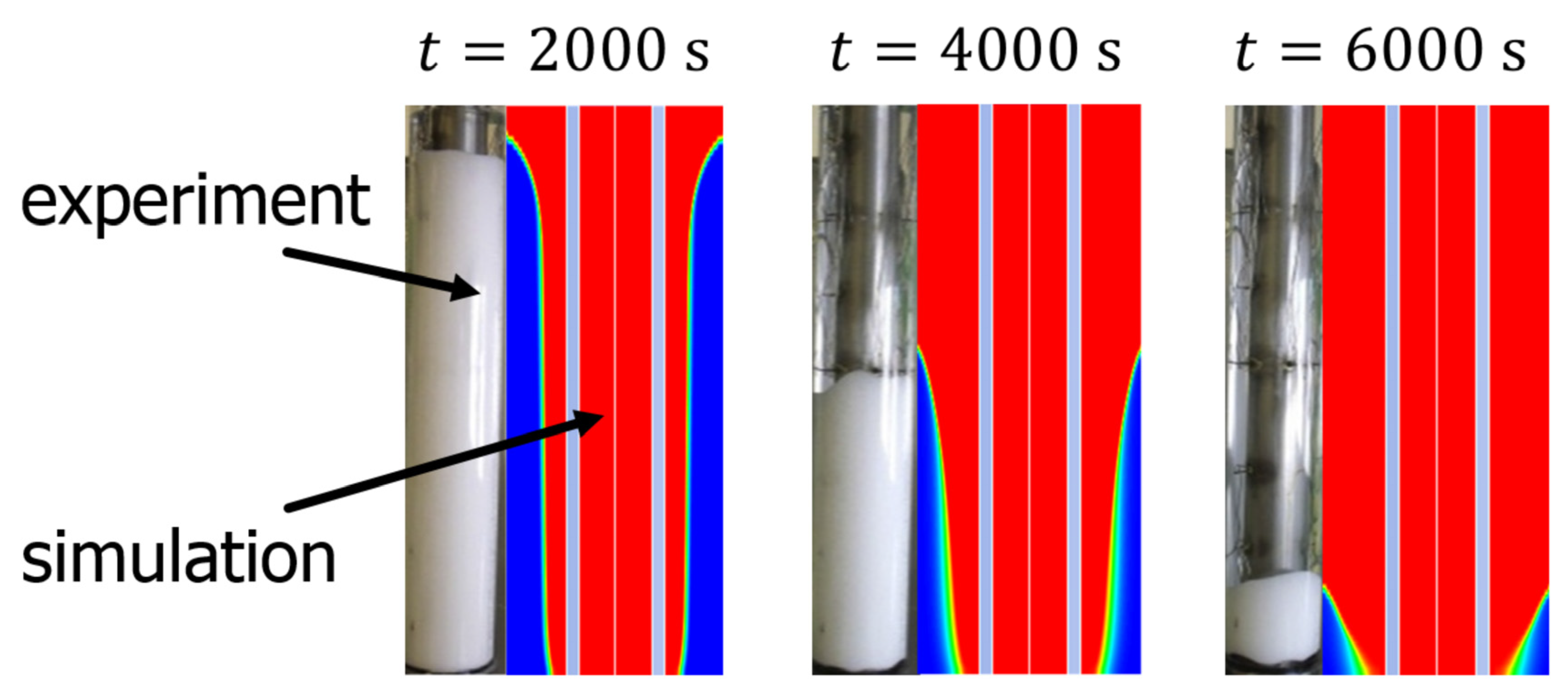
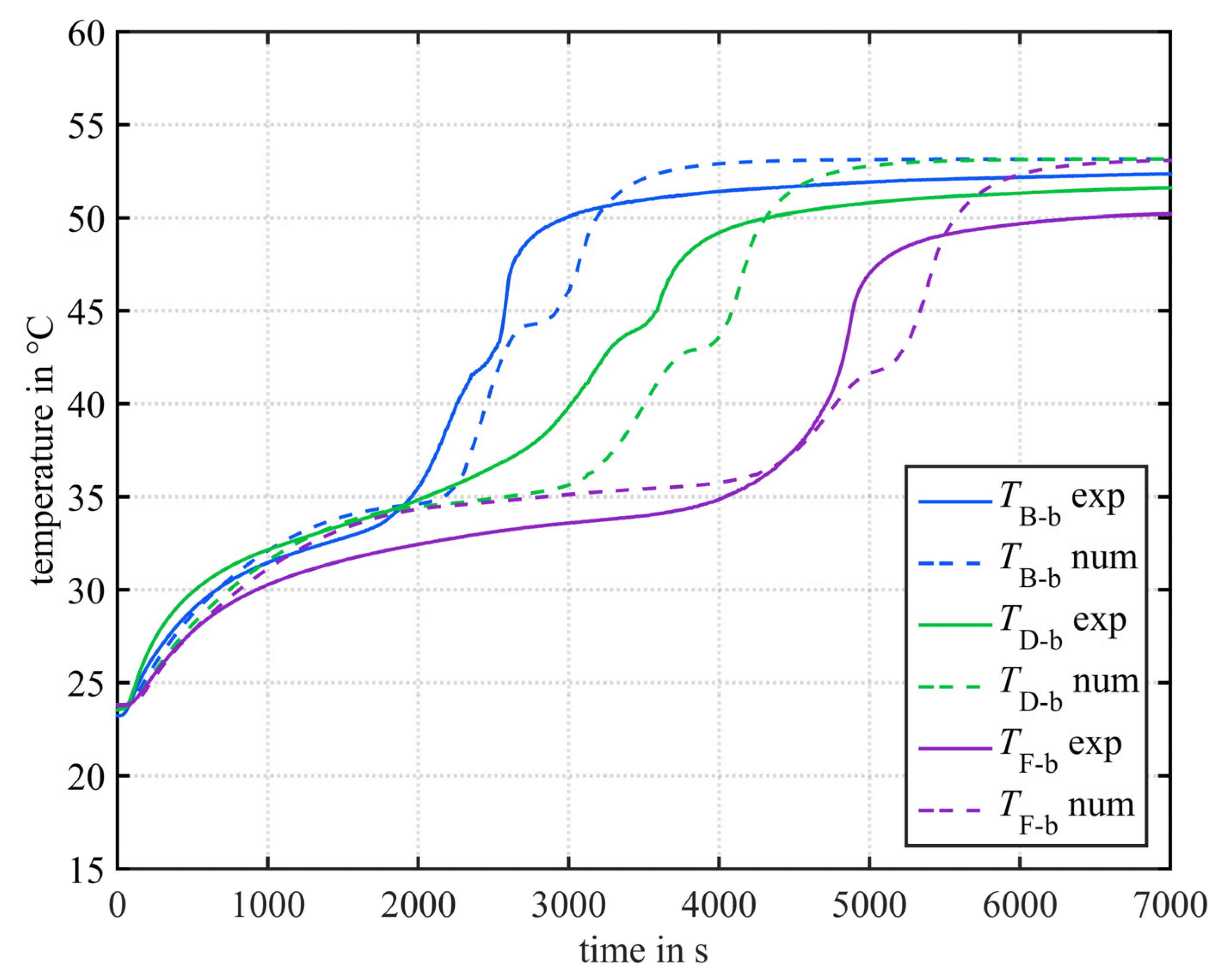
3.1. Validation and Independency Studies

All independency studies and the validation were performed for the charging process. The influence of the mesh was studied by three times refining an initial mesh of 12,200 cells with a factor of 1.2 in both spatial directions and by three times coarsening with a factor of 1.5 in both spatial directions. The maximum difference in the global liquid fraction (at 2000, 4000, and 6000 s) between the 12,200 cells mesh to the next finer one was only 0.63%, but the simulation time increased by about 40 h. Therefore, for all other simulations, a mesh with 12,200 cells was taken.

For solving the pressure-velocity coupling, the SIMPLE and the PISO scheme as well as a PISO scheme with extrapolation—here called PISO-extra—were investigated. No difference was found in the liquid fraction for the different schemes, but the PISO-extra scheme was the fastest one in terms of computational time and almost 46% faster than the slowest one (SIMPLE). All following simulations were performed with the PISO-extra scheme.

The influence of the discretization of the convective fluxes within the momentum and energy equation was studied as well. Three methods were analyzed (in an ascending sequence according to their order): Power-Law, Second-Order-Upwind, and Quadratic Upstream Interpolation for Convective Kinematics (QUICK). The maximum difference in the global liquid fraction at 2000, 4000, and 6000 s was about 4.5% between the Power-Law and the Second-Order-Upwind scheme, and about 0.5% between the Second-Order-Upwind and the QUICK scheme. Accordingly, the QUICK scheme was used for all subsequent simulations.

The time step was first calculated according to the ANSYS Fluent Guide [35] for natural convection to 0.0213 s. Subsequently, the time step was gradually increased and the results were compared. The simulation ran stable as long as a time step $\le 0.2\mathrm{s}$ was chosen and there were no visible differences in the results for all stable simulations. In addition, a reduction of the simulation time of about 85% occurred by increasing the time step from 0.0213 to 0.2 s. For this reason, a time step of 0.2 s is used for all further simulations.

Finally $C_{\mathrm{I}}$ was varied from ${10}^5$ to ${10}^8$. It was seen that the results are not significantly different for a $C_{\mathrm{I}}$ of ${10}^7$ and ${10}^8$. Therefore, a value of ${10}^7$ was chosen.

To validate the model, numerical results were compared to melting experiments described in Longeon et al. [31]. As depicted in Figure 3, the height of the solid PCM in contact with the outer tube is in good agreement between experiment and simulation. Due to the opacity of the solid PCM, the shape of the melting front cannot be analyzed optically. A comparison of the temperature curves over time, though, shows some significant deviations. This is illustrated in Figure 4 for temperature curves from measuring points with an identical height, and in Figure 5 for temperature curves from measuring points with an identical radius. Besides, the absolute mean discharging power up to 7000 s is 10.6% higher in the simulation compared to the experiment and the charging power is 29.9% smaller in the simulation. In order to better assess the reason for these deviations, a sensitivity analysis is performed in the following chapter.

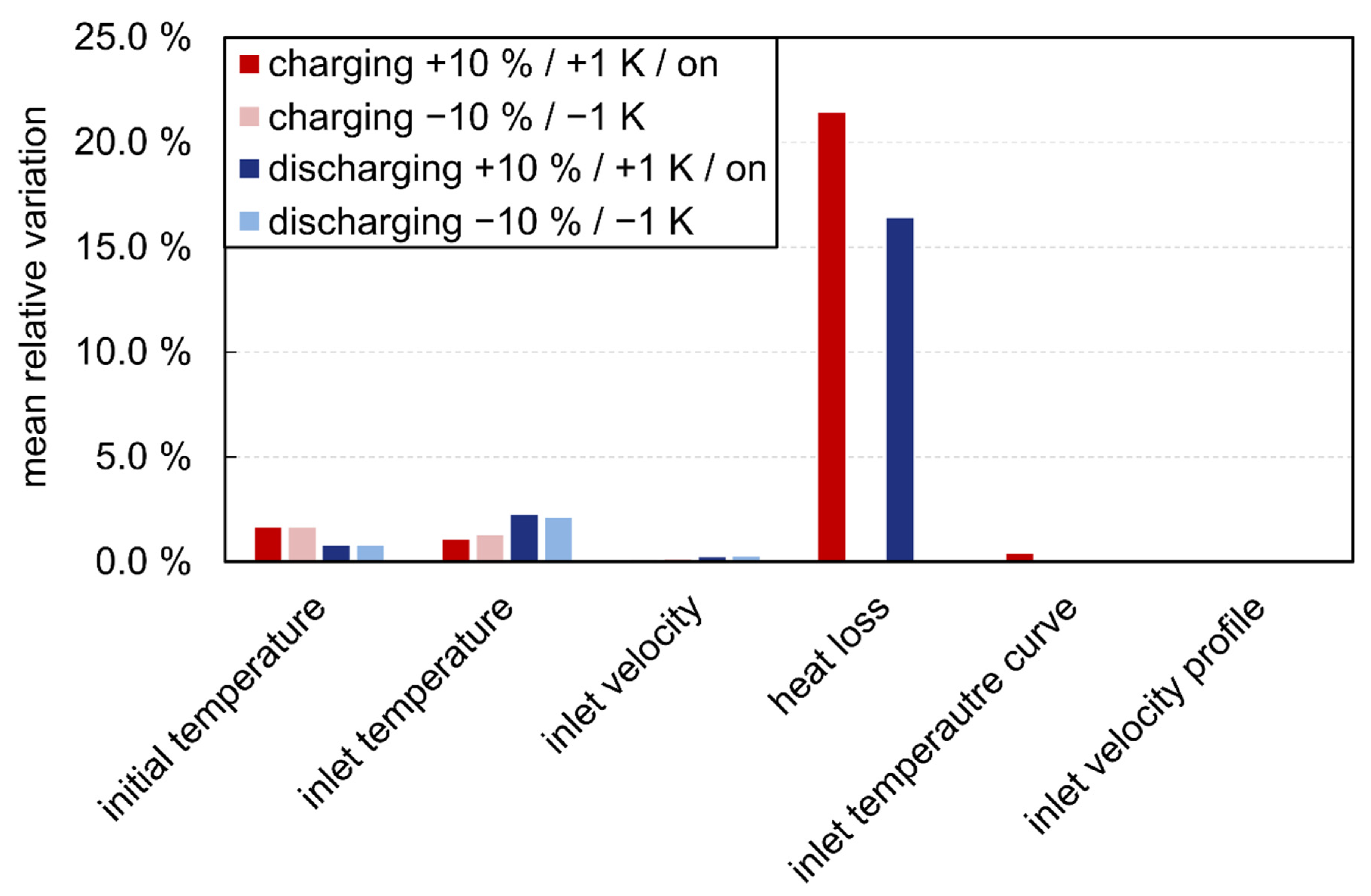
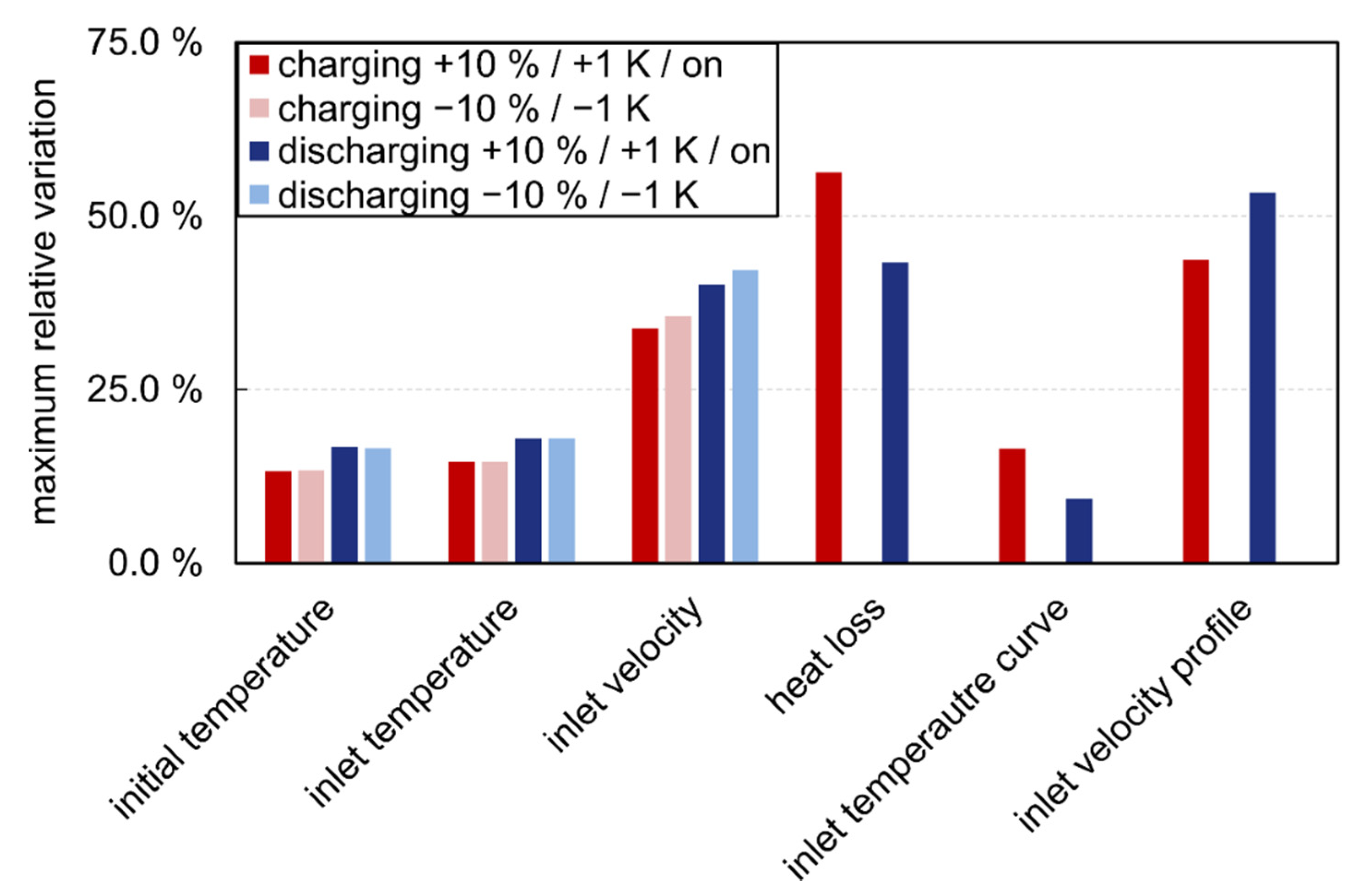
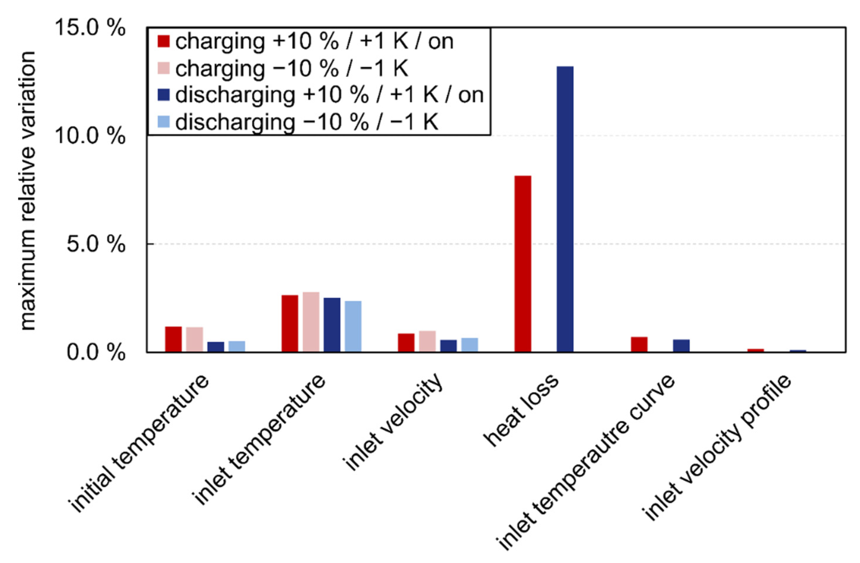
3.2. Sensitivity Analysis

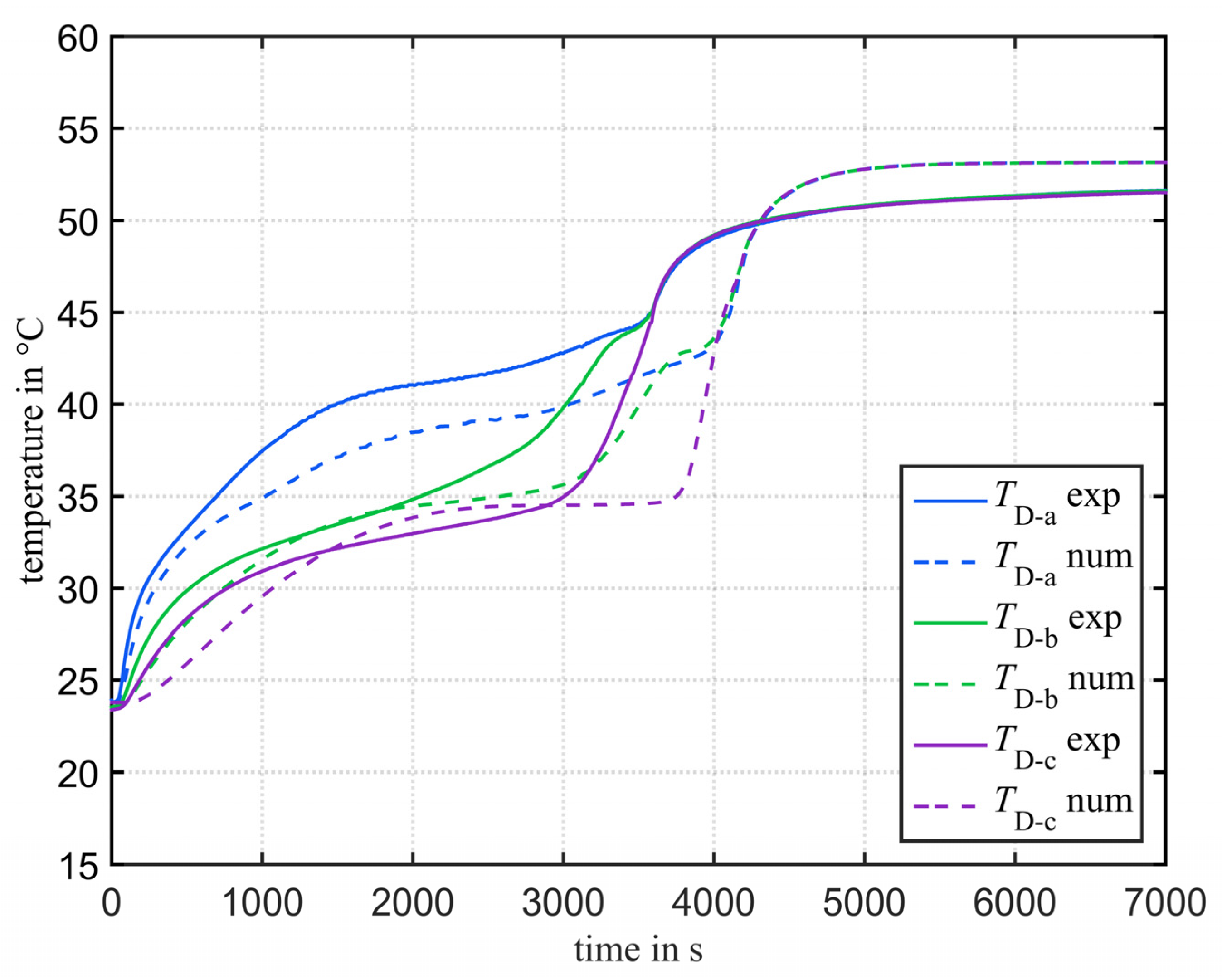
3.2.1. Temperature Measuring Position

The influence of the temperature measuring position is studied first. A variation of the measurement position in the numerical model by ±1 mm in radial position results in a difference in the PCM temperature of up to 5.2 K and a difference in the temporal mean of the temperature of up to 1.0 K. Varying the position in vertical direction by ±1 mm leads to much lower differences of a maximum deviation of less than 0.5 K and only about 0.03 K temporal mean deviation.

Table A2. Temporal mean, maximum, and standard deviation of the temperature measurements with a varied measurement point position with respect to the reference position.

		Point B-b	Point D-a	Point D-b	Point D-c	Point F-b	Mean	Unit
radial +1 mm	mean	−0.33	−0.67	−0.38	−0.21	−0.41	−0.40	K
	maximum	4.30	2.24	2.84	5.21	2.16	3.35	K
	standard deviation	0.74	0.84	0.62	0.70	0.49	0.68	K
radial −1 mm	mean	0.38	1.01	0.44	0.26	0.49	0.52	K
	maximum	3.61	3.10	2.09	4.32	1.47	2.92	K
	standard deviation	0.74	1.10	0.60	0.68	0.48	0.72	K
vertical +1 mm	mean	0.03	0.02	0.02	0.02	0.03	0.03	K
	maximum	0.32	0.33	0.30	0.44	0.37	0.35	K
	standard deviation	0.07	0.05	0.05	0.07	0.06	0.06	K
vertical −1 mm	mean	−0.03	−0.02	−0.02	−0.02	−0.03	−0.03	K
	maximum	0.32	0.33	0.30	0.44	0.37	0.35	K
	standard deviation	0.07	0.05	0.05	0.07	0.06	0.06	K

in the Appendix A shows the maximum and mean values as well as the standard deviation of the temperature differences introduced due to the measurement point variation. The outcome that a variation of the measurement position in radial direction has a much higher effect than a vertical variation can be explained by the almost vertical melting front (see Figure 3). The isotherms within the solid and the liquid PCM follow, to a large extent, the shape of the melt front and, therefore, a small and a large temperature gradient result in vertical and radial directions, respectively.

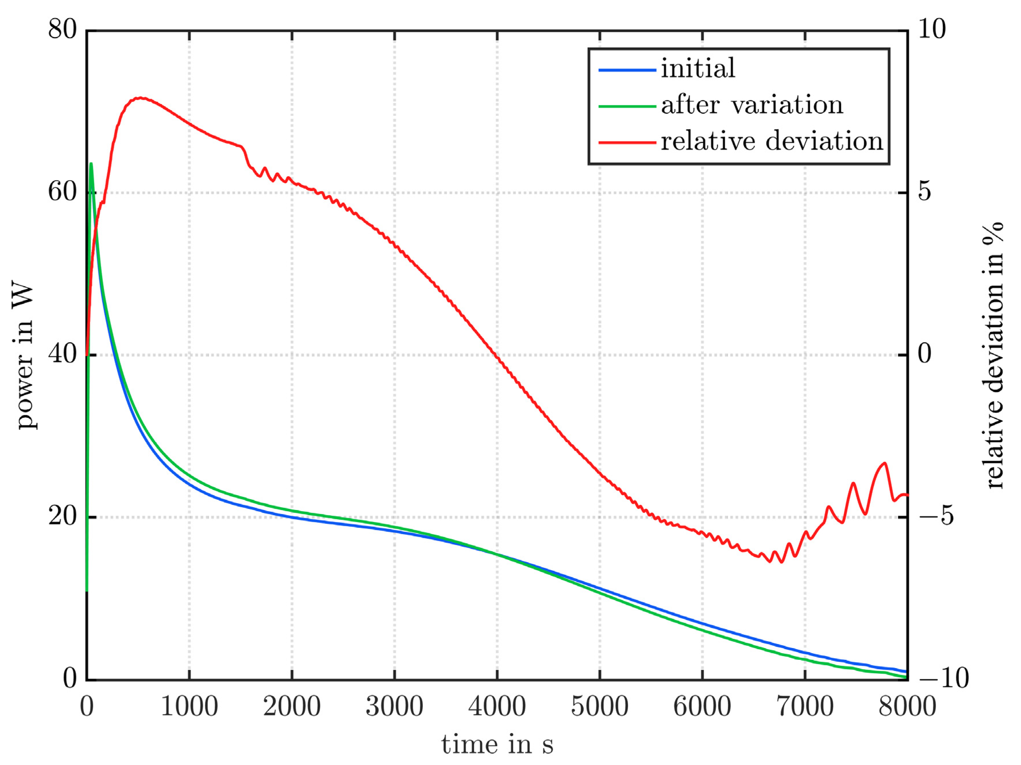
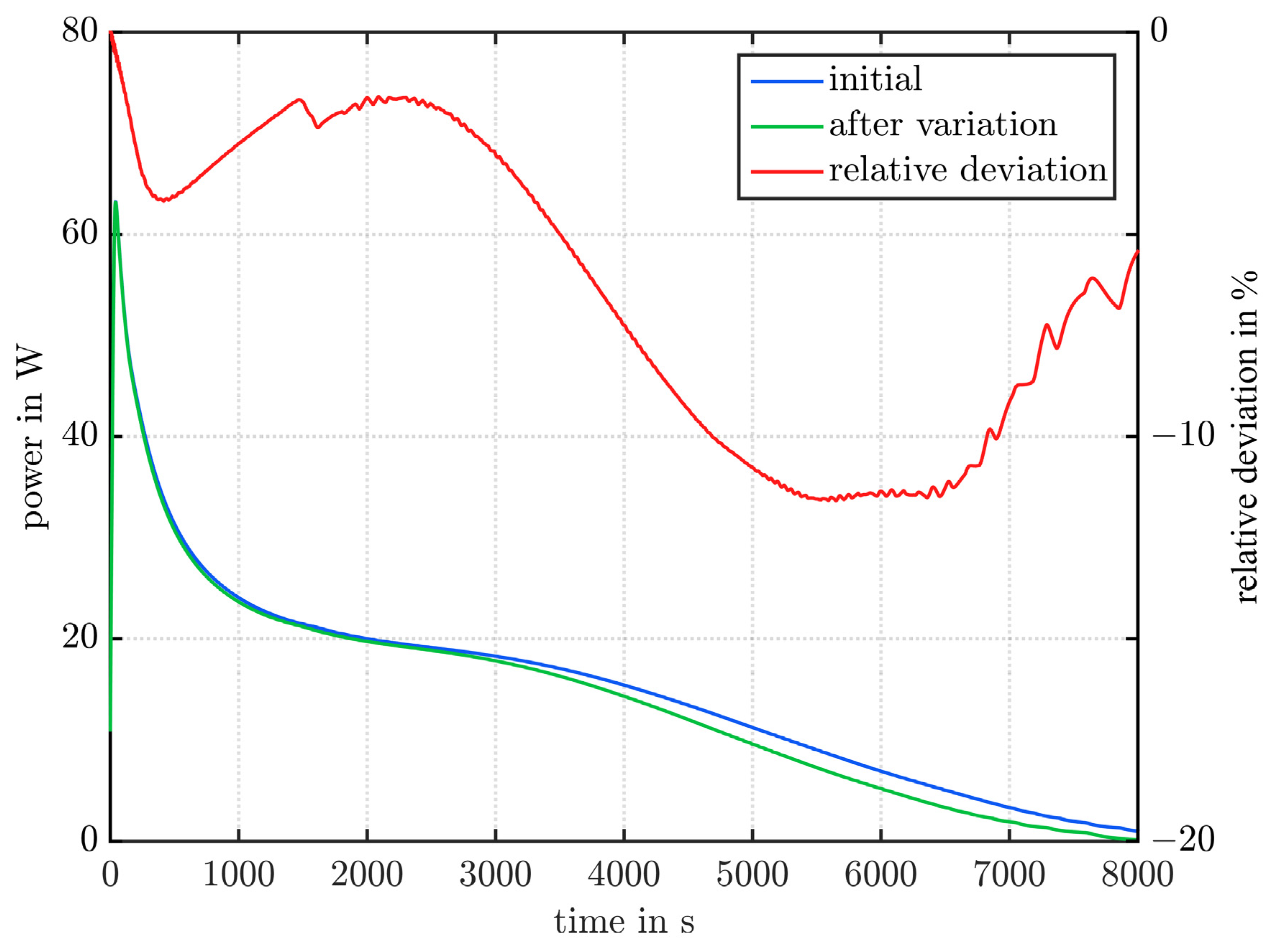
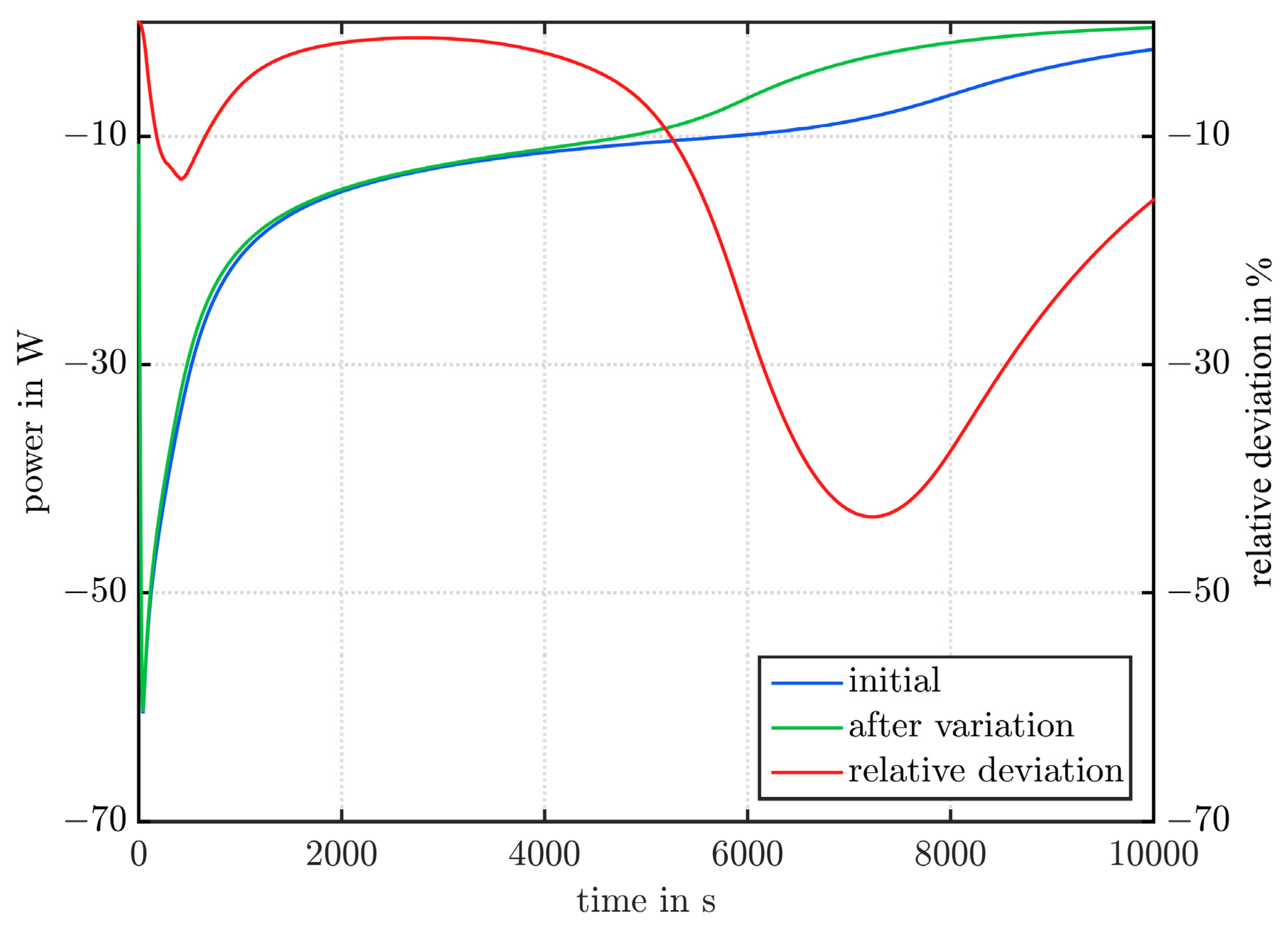
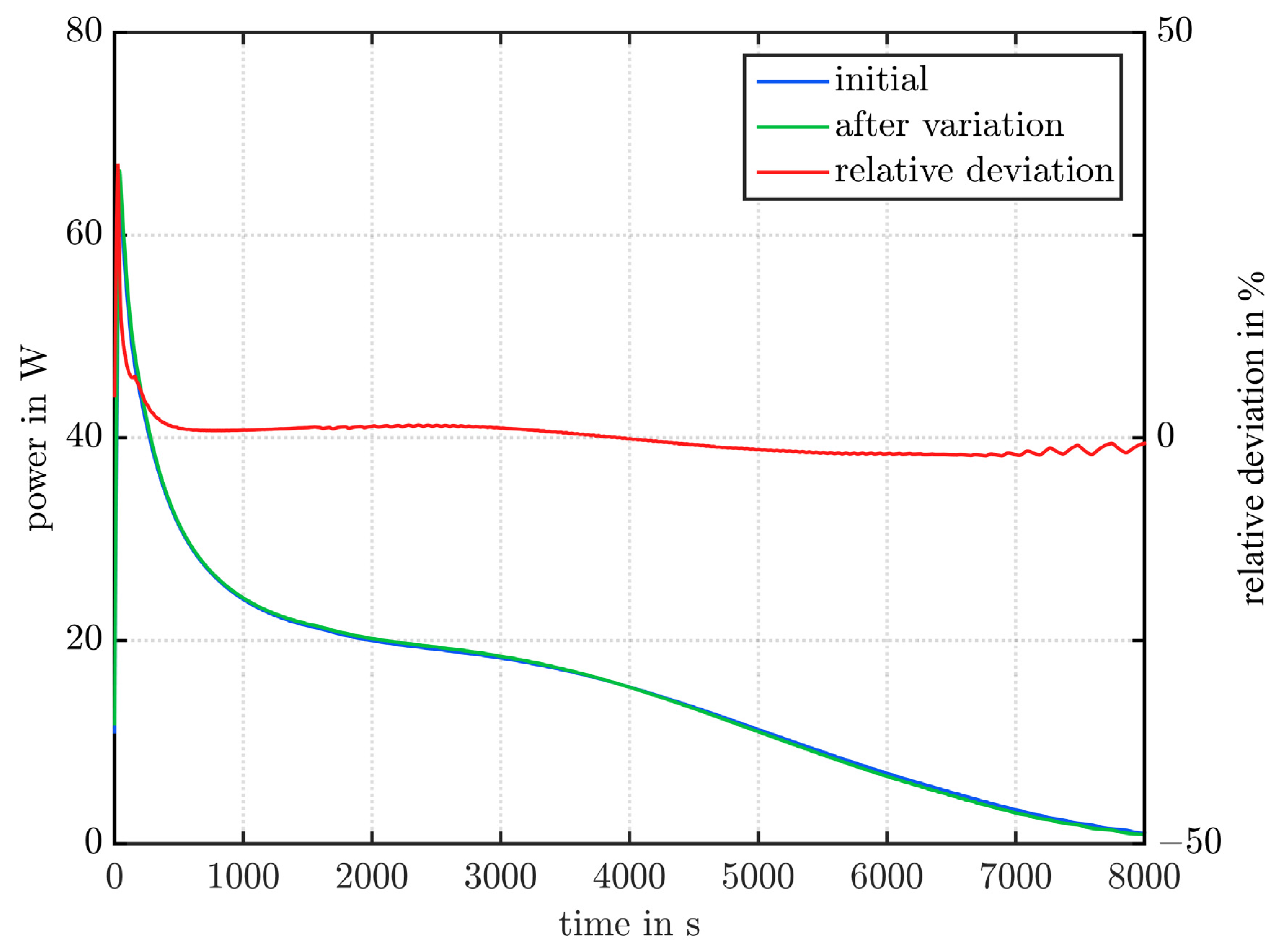
3.2.2. Material Properties

The outcome of the variation of the material properties is presented hereafter and an overview of the results including the sign of the resulting changes in the mean power can be found in the Appendix A in

Table A3. Overview of the influence on the magnitude of the mean power for all varied material properties as well as boundary and initial conditions. The charging and discharging power is always defined positive.

	Charging		Discharging
	+10% +1 K on	−10% −1 K off	+10% +1 K on	−10% −1 K off
$\rho$	8.64%	−9.20%	7.09%	−8.02%
$c_s$	1.64%	−1.65%	1.39%	−1.51%
$c_l$	1.08%	−1.09%	0.70%	−0.70%
$\lambda$	0.24%	−0.50%	1.16%	−1.76%
$L$	5.94%	−6.37%	5.24%	−5.60%
$\eta$	−0.05%	0.05%	0.00%	0.00%
$\beta$	0.05%	−0.06%	0.00%	0.00%
$C_{\mathrm{I}}$	−0.01%	0.01%	0.00%	0.00%
$T_{\mathrm{m}}$	0.36%	−0.63%	1.31%	−1.45%
$T_l-T_s$	−0.06%	0.04%	0.12%	−0.20%
inlet velocity	0.09%	−0.12%	0.21%	−0.25%
initial temperature	−1.64%	1.64%	0.79%	−0.79%
inlet temperature	1.05%	−1.27%	−2.23%	2.10%
heat loss	21.42%	−	−16.39%	−
inlet temperature curve	0.40%	−	0.06%	−
inlet velocity profile	0.01%	−	−0.04%	−

. Figure 6 shows the absolute relative variation of the mean power for charging and discharging with varied material properties. The variation of the density has the highest influence within the material properties of about 7.1% to 9.2%, followed by the melting enthalpy with 5.2% to 6.4%. The influence of the melting temperature, heat capacities and heat conductivity is always below 2.0%, but still noticeable. The influence is higher during charging compared to discharging for density, melting enthalpy as well as heat capacities and lower for heat conductivity and melting temperature. A variation of $\eta ,$ $\beta ,$ the Darcy constant $C_{\mathrm{I}}$ and the mushy zone width $T_{\mathrm{l}}-T_{\mathrm{s}}$ by $\pm 10\%$ and $\pm 1\mathrm{K}$, respectively, has almost no influence on the mean power for the chosen conditions. In general, the impact is somewhat higher when lowering the parameter than when increasing it.

The maximal absolute relative influence of a variation in material properties on the charging and discharging power over time is depicted in Figure 7. The highest influencing parameter is density with 13.3% to 18.4%, followed by melting enthalpy with 10.8% to 13.6%, heat conductivity with 7.9% to 9.8% and melting temperature with 5.5% to 7.8%. All other material properties have always an influence of less than 6.0% and $C_{\mathrm{I}}$ has almost no impact. For $\rho ,$ $\lambda ,$ $L,$ $c_{\mathrm{s}}$ and especially $c_l$ the influence is higher during discharging than during charging and for $T_m$ it is vice versa. Again, the impact is, in general, somewhat higher when lowering the parameters than when increasing them.

The maximal absolute relative influence on the global liquid fraction is presented in Figure 8 as a function of the variation in material properties. The highest influencing parameter is density with a variation of 4.3% to 4.8%, followed by melting enthalpy with 3.3% to 4.2%, melting temperature with 2.5% to 3.7%, and thermal conductivity with 2.6% to 3.6%. For the other parameters, the influence is always below 2.0% and $C_{\mathrm{I}},$ $\eta$ and $\beta$ as well as $c_l$ during charging and $c_s$ during discharging have almost no impact.

By analyzing the results as a whole, the material properties can be divided into three groups:

• Material properties that have no, or only little effect, if they are varied like indicated here: only $C_{\mathrm{I}}$ has an influence that is always below 1% (maximum of 0.12%). Here, one has to keep in mind that $C_{\mathrm{I}}$ is varied by several orders of magnitude in literature, and not only by ±10%.
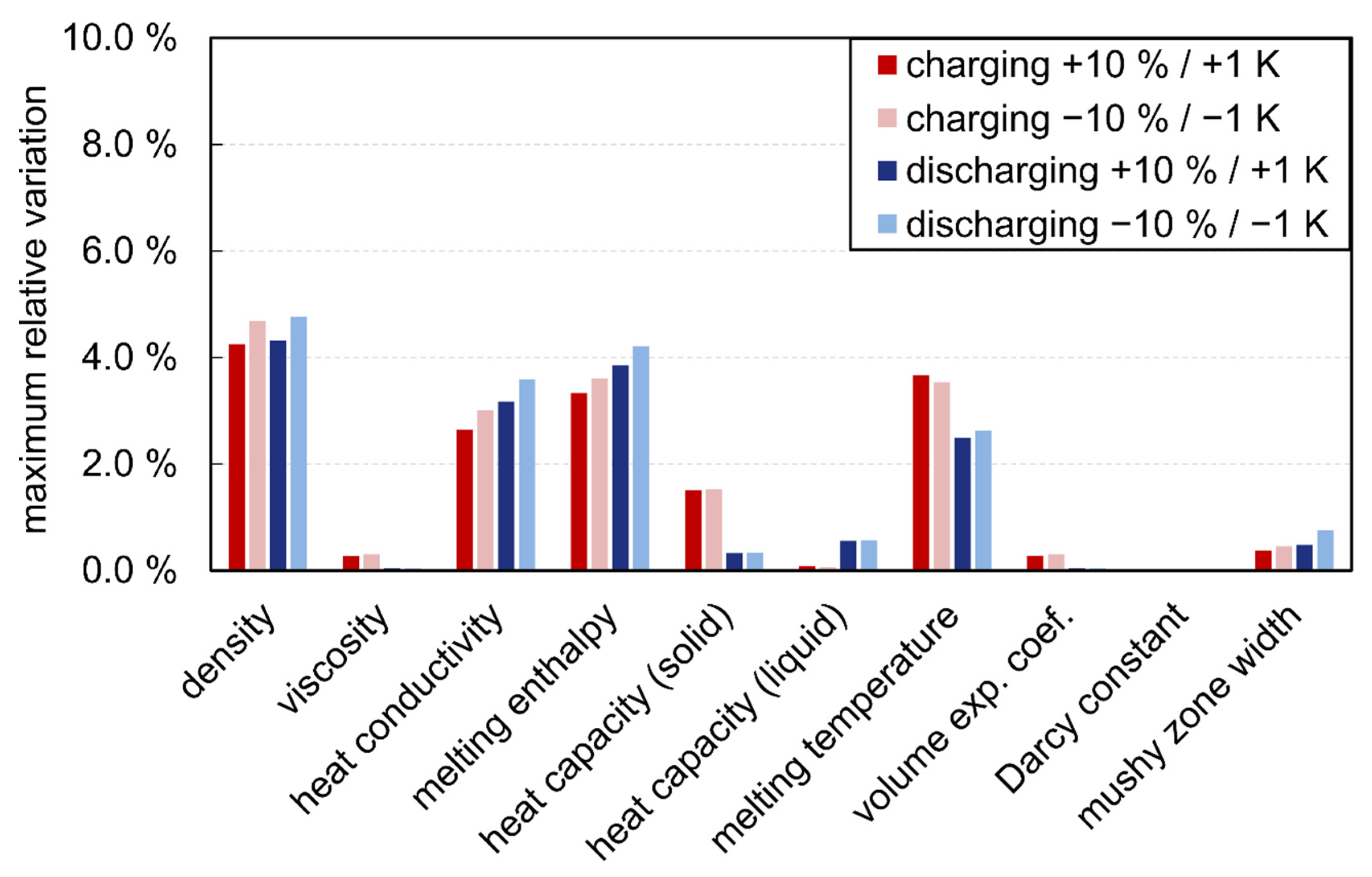
• Material properties that have an influence on the power and the global liquid fraction, but none on the mean power (i.e., the total heat transferred): the material properties $\eta ,$ $\beta ,$ $\lambda$ and $T_{\mathrm{l}}-T_{\mathrm{s}}$ mainly influence the maximum deviations and not the mean power. The reason why $\lambda$ also has a slight influence on the average output is that the storage system can still absorb or release a certain amount of sensible heat at the end of charging and discharging.
• Material properties that also influence the mean power (i.e., the total heat transferred): all remaining material properties ($\rho ,$ $L,$ $c_l,$ $c_s,$ $T_m$) also affect the mean power when varied, but $c_l,$ $c_s$ and $T_m$ only slightly.

The power over time curve during charging is shown in Figure 9 for the reference case and an increased melting enthalpy. Throughout the whole simulation, the deviation is positive—the mean power is increased. In contrast, Figure 10 shows that an increase in thermal conductivity (also for charging) leads to a different type of deviation. First, the power is increased for the variation compared to the reference, but later it decreases—the mean power is only affected slightly. The same phenomenon can be seen for discharging and the contrary effect can be seen for lowering the melting enthalpy and heat conductivity (Figure A1 and Figure A2 in the Appendix A). This behavior is, in general, identical for all material properties that either affect only the maximum deviation of the power and the global liquid fraction or also the mean power.

3.2.3. Boundary and Initial Conditions

Finally, the outcome of the variation of the initial and boundary conditions is presented and again an overview, including the sign of the resulting changes in the mean power is shown in the Appendix A in Table A3. When analyzing these results, one has to keep in mind that in general the parameters are varied by ±1 K and ±10%, but the heat losses, the inlet temperature (constant value vs. curve) and the inlet velocity (constant vs. parabolic profile) are varied in an on/off manner. Therefore, the influence is in general in a plus and minus direction, and only in one direction for the parameters with on/off variations. Consequently, the later presented ranking is based on a comparison of a mean of the variation by +1 K and −1 K or +10% and −10% with a variation from off (e.g., constant value) to on (e.g., profile).

Figure 11 shows the mean deviation of the charging and discharging powers. The highest absolute influence can be seen for the heat losses with 21.4% and 16.4% during charging and discharging, respectively. The initial temperature and the inlet temperature have an influence of 0.8% to 2.2% on the mean power when varied by ±1 K. All other variations of the boundary conditions (inlet velocity, inlet temperature curve and inlet velocity profile) have almost no influence on the mean power.

In Figure 12, the maximum deviations of the charging and discharging power are presented for the variations of the initial and boundary conditions. The highest influence can be seen for the heat loss with 43.3% and 56.3% followed by the inlet velocity profile with 43.7% and 53.4% and the inlet velocity with 33.8% to 42.2%. The variation of the remaining initial and boundary conditions has an influence of 9.3% to 18.0%. The power during the charging and the discharging is depicted in the Appendix A in Figure A3 and Figure A4 respectively for the reference case and the one with heat losses. As a comparison, the charging process with an inlet velocity variation of +10% is also examined in the Appendix A in Figure A5. In general, for all initial and boundary condition variations—except for the heat losses—the largest deviations occur only for a very short time interval at the beginning of the charging and discharging process (see e.g., Figure A5). This is also the reason why they have only a rather small effect on the average performance.

The maximal deviations of the global liquid fraction are shown in Figure 13 when varying the initial and boundary conditions. The heat loss has the greatest influence with 8.2% to 13.2%, followed by the inlet temperature with 2.4% to 2.8%. All other variations of the initial and boundary conditions have a minimal impact of 0.1% to 1.2% on the maximal deviation of the global liquid fraction.

Lastly, a comparison between experimental and numerical results with and without heat losses is performed on the mean power during the charging and discharging process until 7000 s. For charging, the achieved absolute mean powers are 26.2 W, 18.3 W, and 20.7 W for the experiment, the simulation without heat losses, and the simulation with heat losses, respectively. In the same order, the absolute mean powers during discharging are 14.1 W, 15.6 W, and 14.5 W. This leads to an absolute relative deviation of the simulation with heat losses from the experiment of 20.8% and 2.5% for charging and discharging, respectively. This is a distinctive decrease compared to the numerical results without heat losses; here the absolute relative difference was 29.9% for charging and 10.6% for discharging.

4. Comparison with Previous Studies

In this section, the outcome of the current study is compared with results from literature. It has turned out that a simple one-to-one comparison should not be done, as the initial variables, the applications and the number of varied parameters as well as their variation range may be very different. In addition, Dolado et al. [27] and Mazo et al. [28] used a hypercube sampling and assumed a normal distribution of the varied parameter. In contrast, the analysis of Zsembinszki et al. [30] and the study presented here are based on a simple variation with respect to a reference case. Nevertheless, a comparison will still give more insights into the interdependencies and may reveal details for the need for future research.

Therefore, in

Table 5. Comparison of the most influential parameters and their assumed variation.

Study	Output	1.	2.	3.	4.	5.
Dolado et al. [27]	mean power deviation	$T_{\mathrm{m}}$ $\pm 1\mathrm{K}$	$\dot{V}$ $\pm 6.14\%$	$T_{\mathrm{in}}$ $\pm 0.6\mathrm{K}$	$d$ $\pm 10\%$	$L$ $\pm 10\%$
Zsembinszki et al. [30]	mean absolute power deviation	$T_{\mathrm{in}}$ $\pm 1\mathrm{K}$	$T_{\mathrm{m}}$ $\pm 1\mathrm{K}$	$\rho$ * $\pm 5\%$	$\frac{\partial h}{\partial T}$ * $\pm 5\%$	$\alpha$ $\pm 30\%$
	mean power deviation	$T_{\mathrm{in}}$ $\pm 1\mathrm{K}$	$\rho$ ** $\pm 5\%$	$\frac{\partial h}{\partial T}$ ** $\pm 5\%$	$T_{\mathrm{m}}$ $\pm 1\mathrm{K}$	${\rho }_{\mathrm{HTF}}$ *** $\pm 5\%$
Mazo et al. [28]	saving in yearly energy consumption	$T_{\mathrm{m}}$ $\pm 1\mathrm{K}$	$\lambda$ $\pm 10\%$	$L$ $\pm 10\%$	$\rho$ $\pm 2\%$	$c$ $\pm 5\%$
this study	mean power deviation	${\dot{Q}}_{\mathrm{loss}}$ on/off	$\rho$ $\pm 10\%$	$L$ $\pm 10\%$	${\mathrm{T}}_{\mathrm{in}}$ $\pm 1\mathrm{K}$	$c_s$ $\pm 10\%$
	maximum power deviation	${\dot{Q}}_{\mathrm{loss}}$ on/off	$u_{\mathrm{in},\mathrm{profile}}$ On/off	$u_{\mathrm{in}}$ $\pm 10\%$	$T_{\mathrm{in}}$ $\pm 1\mathrm{K}$	$\rho$ $\pm 10\%$
	maximum global liquid fraction deviation	${\dot{Q}}_{\mathrm{loss}}$ on/off	$\rho$ $\pm 10\%$	$L$ $\pm 10\%$	$\lambda$ $\pm 10\%$	$T_{\mathrm{m}}$ $\pm 1\mathrm{K}$

* For the mean absolute power deviation in Zsembinszki et al. [28], $\rho$ and $\frac{\partial h}{\partial T}$ are equally important; ** For the mean power deviation in Zsembinszki et al. [28], $T_{\mathrm{in}}$, $\rho$ and $\frac{\partial h}{\partial T}$ are equally important; *** For the mean power deviation in Zsembinszki et al. [28], $c_{HTF}$ is equally important as ${\rho }_{HTF}$.

, the most influential parameters are listed together with their assumed variation range for all studies mentioned above. On average, $T_{\mathrm{m}}$ is the most influential parameter in the studies from literature. Whereas, the heat loss is the most dominant parameter in this study. It is worth mentioning that the effect of heat loss is not investigated in the studies found in literature and might be distinct smaller due to proper insulation. A comparison of all studies that are investigating the influence on the mean power shows that the ranking of the most influential material properties is still different even though the influenced parameter is identical. In the present study, $\rho$ and $L$ are the most relevant material parameters and in the literature these are $T_{\mathrm{m}}$ and $L$ [27] or $\frac{\partial h}{\partial T}$ and $\rho$ as well as $T_{\mathrm{m}}$ [30] (the ranking for the deviation of the mean power is somewhat different from the ranking based on the deviation of the mean absolute power). Dolado et al. [27] also studied, among other parameters, the time until the output temperature reaches a certain temperature threshold. Here, the ranking is again different from the one when looking at the mean power. The ranking given by Mazo et al. [28] is different for the heating energy demand than for the cooling demand and the ranking depends on the PCM layer thickness, too. The corresponding ranking in Table 5 is the one given in the conclusion section of the original paper [28].

Not only the ranking of the most important parameters varies between and within the different studies but also the overall impact of the variations varies widely. Mazo et al. [28] report that the yearly energy demand for cooling the studied test cell changes by about ±10% when all parameters are varied together. Moreover, for a variation of all parameters, Dolado et al. [27] have found that this causes differences in the mean power of about ±3.75%. In contrast, Zsembinszki et al. [30] state that changing $T_{\mathrm{in}}$ by ±1 K already leads to a shift of the mean absolute power by about ±11%. Similarly, the results of the current study revealed that a variation of $\rho$ by ±10% leads to changes in the mean power of about ±8%, and accounting for the heat losses or not leads to a difference in the mean power of 19.4% and 13.5% for charging and discharging, respectively.

5. Conclusions

Within this paper, a basic sensitivity analysis is performed to understand the sources of uncertainties within a CFD simulation of a vertical shell-and-tube LTESS during charging and discharging. First, the influence of several numerical parameters was investigated, and it was concluded that the major part of the uncertainties must be found elsewhere. Consequently, a sensitivity analysis of the material properties, as well as boundary and initial conditions and measurement positions, was carried out. In order to keep the simulation effort within limits, a simple analysis was performed in which the parameters were varied by a certain value in relation to a reference case. Ten material properties were varied by either $\pm 10\%$ or $\pm 1\mathrm{K}$, and six boundary and initial conditions by either $\pm 10\%$, $\pm 1\mathrm{K}$, or in an on/off manner, and the resulting deviation of the mean power, as well as the maximum deviation of the power and the global liquid fraction, were analyzed. In addition, the position of the temperature measurements within the simulation was varied by $\pm 1\mathrm{mm}$. The most important results are:

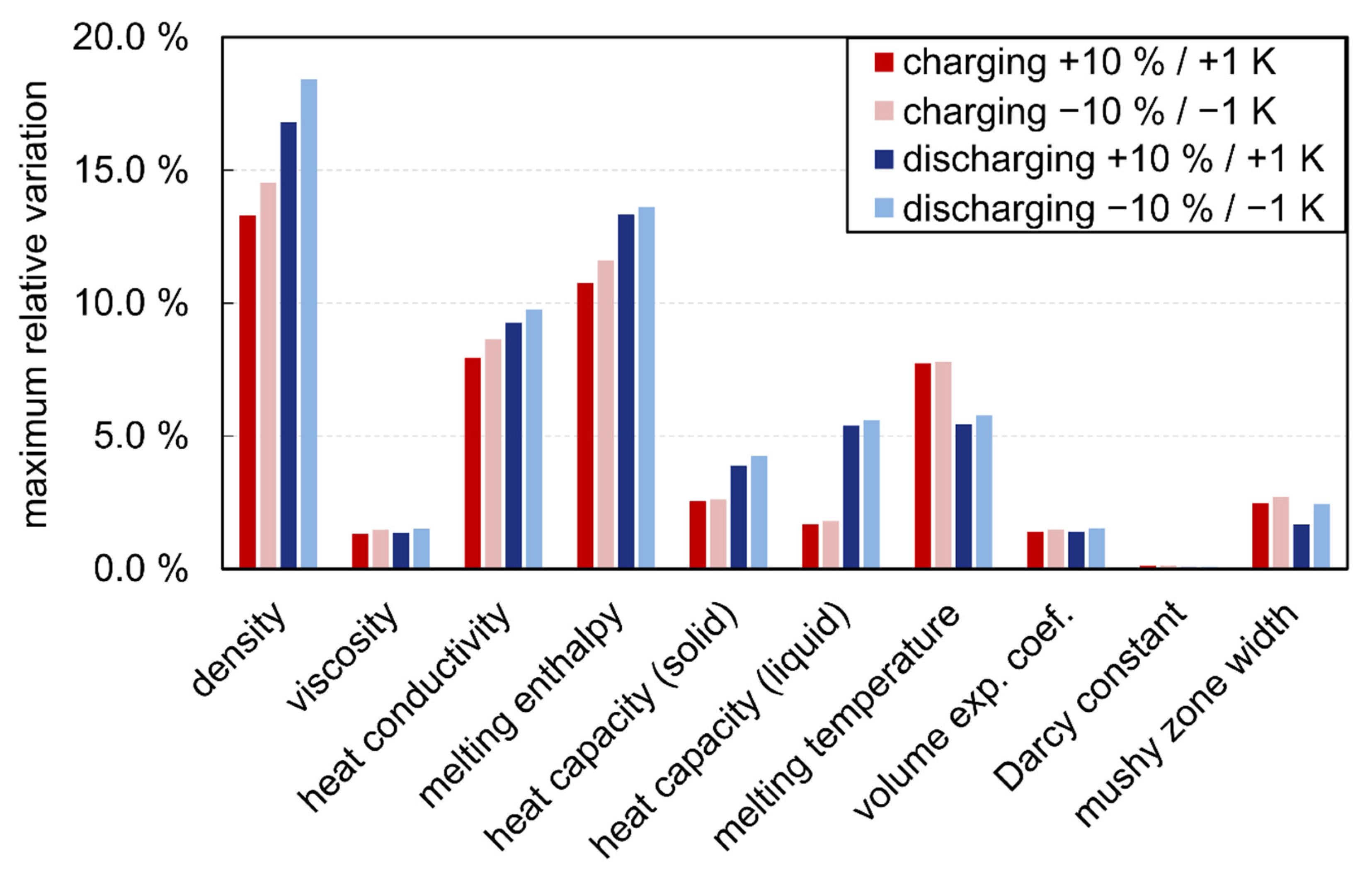
• The variation of the material properties had a very large effect on the power and the global liquid fraction. In conclusion, uncertainties in the material properties may affect the results of a CFD simulation of a LTESS significantly.
• The material properties can be subdivided into three groups:

  ○

  Material properties that have no or only little effect: only $C_{\mathrm{I}}$ has an influence that is always below 1% (maximum of 0.12%), but one has to keep in mind that it is varied by several orders of magnitude in literature.

  ○

  Material properties that have an influence on the power and the global liquid fraction slope, but none on the mean power: the material properties $\eta ,$ $\beta ,$ $\lambda$ and $T_{\mathrm{l}}-T_{\mathrm{s}}$ mainly influence the maximum deviations and not the mean power.

  ○

  Material properties that also influence the mean power: all remaining material properties ($\rho ,$ $L,$ $c_l,$ $c_s,$ $T_m$) also affect the mean power when varied, but $c_l,$ $c_s$ and $T_m$ only slightly.

• ${\dot{Q}}_{\mathrm{loss}}$ (up to 21.4%), $\rho$ (up to 9.2%) and $L$ (up to 6.4%) have the largest influence on the mean power.
• The ranking of the parameters and the magnitude of the influence is sometimes distinctively different in studies found in literature.
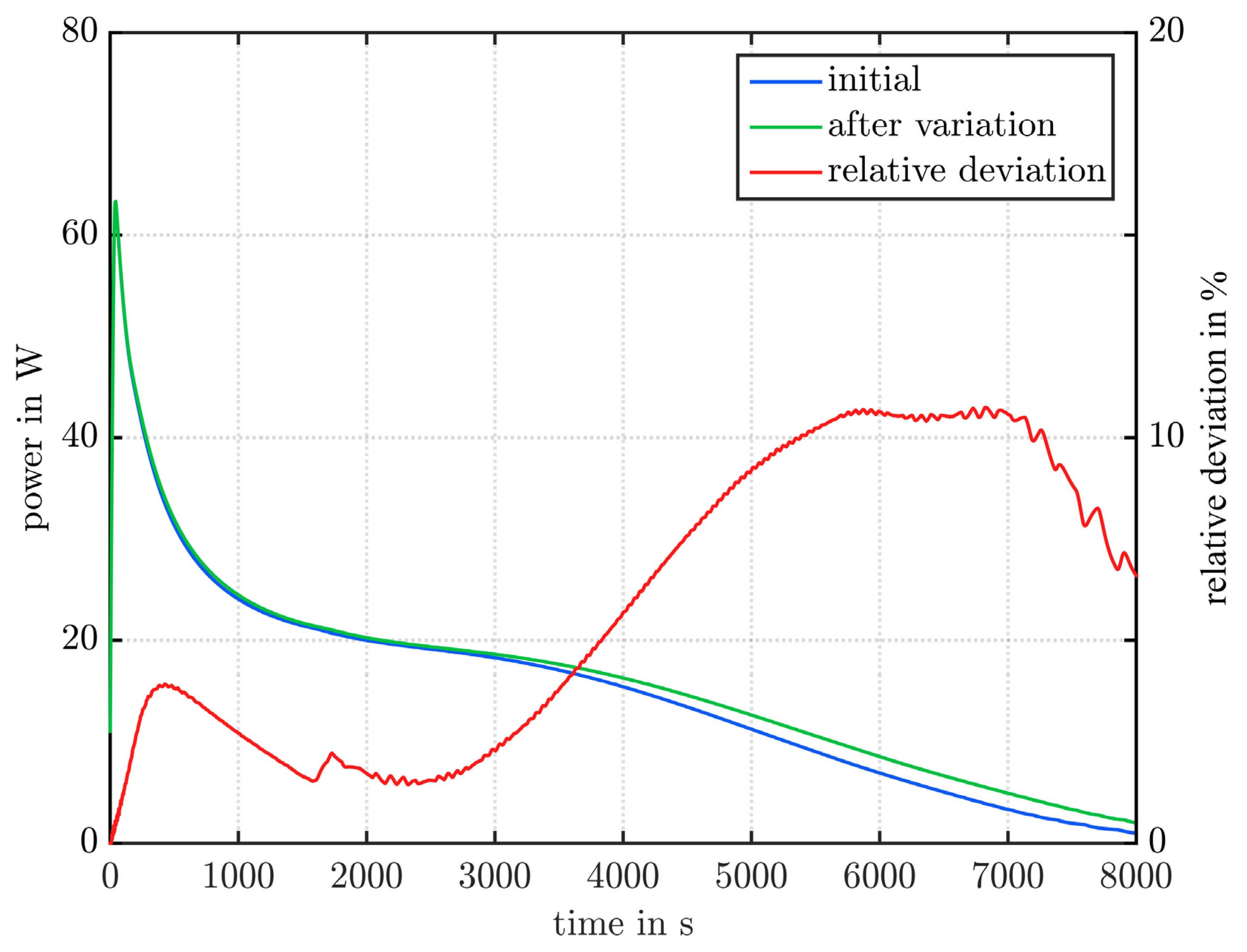
• Comparing the maximum deviation of the power can be misleading as the deviation may only occur as a short peak, and has no effect on the overall performance.
• For the investigated storage configuration and orientation, a radial variation of the temperature measurement position had a much higher impact than a vertical variation. A displacement of the measuring point in radial direction by $\pm 1\mathrm{mm}$ already led to a maximum deviation in the measured temperature of more than 5 K.

The above points indicate that the results of numerical models of latent thermal energy storage units are subject to substantial uncertainties. This is to a large extent a direct consequence of the uncertainties in the applied material properties and the imposed boundary and initial conditions (the order of magnitude of the variation agrees for many parameters with the uncertainties/variations found in literature [3,27,28,30]). In general, however, these uncertainties are not highlighted, but rather hidden. A fair comparison with experiments, including uncertainties like it is performed by Dolado et al. [27] and Mazo et al. [28], is hard to find in literature. One reason for this is certainly the large number of required simulations, which can be an exclusion criterion, especially for CFD studies.

A first next step should include detailed analyses of standard validation experiments. These analyses need to involve the actual uncertainty of the material properties, their temperature dependency, and heat losses, as well as the uncertainties of the experiment. To ensure that the whole parameter range is taken into account, sophisticated sensitivity analysis methods need to be applied. Moreover, the error caused by the Boussinesq approximation and the influence of the chosen switch-off method should be examined in detail.

References

1. Steinmann, W.-D.; Jockenhöfer, H.; Bauer, D. Thermodynamic Analysis of High-Temperature Carnot Battery Concepts. Energy Technol. 2020, 8, 1900895. [Google Scholar] [CrossRef] [Green Version]
2. Mehling, H.; Cabeza, L.F. Heat and Cold Storage with PCM; Springer: Berlin/Heidelberg, Germany, 2008. [Google Scholar]
3. Faden, M.; Höhlein, S.; Wanner, J.; König-Haagen, A.; Brüggemann, D. Review of Thermophysical Property Data of Octadecane for Phase-Change Studies. Materials 2019, 12, 2974. [Google Scholar] [CrossRef] [PubMed] [Green Version]
4. Dutil, Y.; Rousse, D.R.; Salah, N.B.; Lassue, S.; Zalewski, L. A review on phase-change materials: Mathematical modeling and simulations. Renew. Sustain. Energy Rev. 2011, 15, 112–130. [Google Scholar] [CrossRef]
5. Voller, V.R.; Markatos, N.C.; Cross, M. Techniques for account for the moving interface in convection/diffusion phase change. In Numerical Methods in Thermal Problems; Lewis, R.W., Morgan, K., Eds.; Pineridge Press: Swansea, UK, 1985; pp. 595–609. [Google Scholar]
6. Morgan, K. A numerical analysis of freezing and melting with convection. Comput. Methods Appl. Mech. Eng. 1981, 28, 275–284. [Google Scholar] [CrossRef]
7. Gartling, D.K. Finite Element Analysis of Convection Heat Transfer Problems in Phase Change. In Computer Methods in Fluids; Morgan, K., Taylor, C., Brebbia, C.A., Eds.; Pentech: London, UK, 1980; pp. 257–284. [Google Scholar]
8. Brent, A.D.; Voller, V.R.; Reid, K.J. Enthalpy-porosity technique for modeling convection-diffusion phase change: Application to the melting of a pure metal. Numer. Heat Transf. Part A Appl. 1988, 13, 297–318. [Google Scholar]
9. Kheirabadi, A.C.; Groulx, D. The effect of the mushy-zone constant on simulated phase change heat transfer. In Proceedings of the CHT-15: 6th International Symposium on Advances in Computational Heat Transfer, Begell House, Danbury, CT, USA, 25–29 May 2015; p. 22. [Google Scholar]
10. Beust, C.; Franquet, E.; Bédécarrats, J.-P.; Garcia, P.; Pouvreau, J. Influence of the modeling parameters on the numerical CFD simulation of a shell-and-tube latent heat storage system with circular fins. In SOLARPACES 2018: International Conference on Concentrating Solar Power and Chemical Energy Systems; AIP Publishing: Melville, NY, USA, 2019; p. 200007. [Google Scholar]
11. Fadl, M.; Eames, P.C. Numerical investigation of the influence of mushy zone parameter Amush on heat transfer characteristics in vertically and horizontally oriented thermal energy storage systems. Appl. Therm. Eng. 2019, 151, 90–99. [Google Scholar] [CrossRef]
12. Arena, S.; Casti, E.; Gasia, J.; Cabeza, L.F.; Cau, G. Numerical simulation of a finned-tube LHTES system: Influence of the mushy zone constant on the phase change behaviour. Energy Procedia 2017, 126, 517–524. [Google Scholar] [CrossRef]
13. Shmueli, H.; Ziskind, G.; Letan, R. Melting in a vertical cylindrical tube: Numerical investigation and comparison with experiments. Int. J. Heat Mass Transf. 2010, 53, 4082–4091. [Google Scholar] [CrossRef]
14. Ebrahimi, A.; Kleijn, C.R.; Richardson, I.M. Sensitivity of numerical predictions to the permeability coefficient in simulations of melting and solidification using the enthalpy-porosity method. Energies 2019, 12, 4360. [Google Scholar] [CrossRef] [Green Version]
15. Voller, V.R.; Prakash, C. A fixed grid numerical modelling methodology for convection-diffusion mushy region phase-change problems. Int. J. Heat Mass Transf. 1987, 30, 1709–1719. [Google Scholar] [CrossRef]
16. Hu, H.; Argyropoulos, S.A. Mathematical modelling of solidification and melting: A review. Model. Simul. Mater. Sci. Eng. 1996, 4, 371–396. [Google Scholar] [CrossRef] [Green Version]
17. Voller, V.R.; Swaminathan, C.R.; Thomas, B.G. Fixed grid techniques for phase change problems: A review. Int. J. Numer. Methods Eng. 1990, 30, 875–898. [Google Scholar] [CrossRef]
18. Voller, V.R. An overview of numerical methods for solving phase change problems. In Advances in Numerical Heat Transfer; Minkowycz, W.J., Sparrow, E.M., Eds.; Taylor & Francis: New York, NY, USA, 1997; pp. 341–380. [Google Scholar]
19. König-Haagen, A.; Franquet, E.; Faden, M.; Brüggemann, D. Influence of the convective energy formulation for melting problems with enthalpy methods. Int. J. Therm. Sci. 2020, 158, 106477. [Google Scholar] [CrossRef]
20. Tittelein, P.; Gibout, S.; Franquet, E.; Johannes, K.; Zalewski, L.; Kuznik, F.; Dumas, J.-P.; Lassue, S.; Bédécarrats, J.-P.; David, D. Simulation of the thermal and energy behaviour of a composite material containing encapsulated-PCM: Influence of the thermodynamical modelling. Appl. Energy 2015, 140, 269–274. [Google Scholar] [CrossRef]
21. König-Haagen, A.; Franquet, E.; Pernot, E.; Brüggemann, D. A comprehensive benchmark of fixed-grid methods for the modeling of melting. Int. J. Therm. Sci. 2017, 118, 69–103. [Google Scholar] [CrossRef]
22. Galione, P.A.; Lehmkuhl, O.; Rigola, J.; Oliva, A. Fixed-grid numerical modeling of melting and solidification using variable thermo-physical properties—Application to the melting of n-Octadecane inside a spherical capsule. Int. J. Heat Mass Transf. 2015, 86, 721–743. [Google Scholar] [CrossRef] [Green Version]
23. Ben-David, O.; Levy, A.; Mikhailovich, B.; Azulay, A. 3D numerical and experimental study of gallium melting in a rectangular container. Int. J. Heat Mass Transf. 2013, 67, 260–271. [Google Scholar] [CrossRef]
24. Günther, E.; Hiebler, S.; Mehling, H.; Redlich, R. Enthalpy of phase change materials as a function of temperature: Required accuracy and suitable measurement methods. Int. J. Thermophys. 2009, 30, 1257–1269. [Google Scholar] [CrossRef]
25. Arkar, C.; Medved, S. Influence of accuracy of thermal property data of a phase change material on the result of a numerical model of a packed bed latent heat storage with spheres. Thermochim. Acta 2005, 438, 192–201. [Google Scholar] [CrossRef]
26. Feng, G.; Huang, K.; Xie, H.; Li, H.; Liu, X.; Liu, S.; Cao, C. DSC test error of phase change material (PCM) and its influence on the simulation of the PCM floor. Renew. Energy 2016, 87, 1148–1153. [Google Scholar] [CrossRef]
27. Dolado, P.; Mazo, J.; Lázaro, A.; Marín, J.M.; Zalba, B. Experimental validation of a theoretical model: Uncertainty propagation analysis to a PCM-air thermal energy storage unit. Energy Build. 2012, 45, 124–131. [Google Scholar] [CrossRef]
28. Mazo, J.; el Badry, A.T.; Carreras, J.; Delgado, M.; Boer, D.; Zalba, B. Uncertainty propagation and sensitivity analysis of thermo-physical properties of phase change materials (PCM) in the energy demand calculations of a test cell with passive latent thermal storage. Appl. Therm. Eng. 2015, 90, 596–608. [Google Scholar] [CrossRef]
29. Soni, V.; Kumar, A.; Jain, V.K. Modeling of PCM melting: Analysis of discrepancy between numerical and experimental results and energy storage performance. Energy 2018, 150, 190–204. [Google Scholar] [CrossRef]
30. Zsembinszki, G.; Moreno, P.; Solé, C.; Castell, A.; Cabeza, L.F. Numerical model evaluation of a PCM cold storage tank and uncertainty analysis of the parameters. Appl. Therm. Eng. 2014, 67, 16–23. [Google Scholar] [CrossRef] [Green Version]
31. Longeon, M.; Soupart, A.; Fourmigué, J.-F.; Bruch, A.; Marty, P. Experimental and numerical study of annular PCM storage in the presence of natural convection. Appl. Energy 2013, 112, 175–184. [Google Scholar] [CrossRef]
32. Rösler, F. Modellierung und Simulation der Phasenwechselvorgänge in Makroverkapselten Latenten Thermischen Speichern; Logos Verlag Berlin GmbH: Berlin, Germany, 2014. [Google Scholar]
33. VDI. VDI-Wärmeatlas; Springer: Berlin/Heidelberg, Germany, 2013. [Google Scholar]
34. Voller, V.R.; Swaminathan, C.R. General source-based method for solidification phase change. Numer. Heat Transf. Part B Fundam. 1991, 19, 175–189. [Google Scholar] [CrossRef]
35. Fluent, A. Ansys Fluent 15 User’s Guide; ANSYS: Canonsburg, PA, USA, 2013. [Google Scholar]
Figure 1. Basic scheme of the vertical thermocouple positioning in the phase change materials (PCM). HTF: heat transfer fluid.
Applsci 10 06723 g001
Figure 2. Original and simplified geometry used in the numerical simulation.
Applsci 10 06723 g002
Figure 3. Comparison of the height of the solid PCM for the experimental [31] and numerical results during charging (blue indicates solid, red indicates liquid, and yellow as well as green indicate the mushy region). In order to increase the visibility of the numerical results, they were stretched in the radial direction.
Applsci 10 06723 g003
Figure 4. Comparison between experiment (exp) and standard simulation (num) for temperature curves during charging of measurement points with an identical height.
Applsci 10 06723 g004
Figure 5. Comparison between experiment and standard simulation for temperature curves during charging of measurement points with an identical radius.
Applsci 10 06723 g005
Figure 6. Absolute relative variation of the mean power for charging and discharging when varying the material properties by ±10% or ±1 K.
Applsci 10 06723 g006
Figure 7. Absolute maxima of the relative variation of the power for charging and discharging when varying the material properties by ±10% or ±1 K.
Applsci 10 06723 g007
Figure 8. Absolute maxima of the relative variation of the global liquid fraction for charging and discharging when varying the material properties by ±10% or ±1 K.
Applsci 10 06723 g008
Figure 9. Power over time curve for charging of the standard case and the case with an increased melting enthalpy as well as the regarding relative deviation.
Applsci 10 06723 g009
Figure 10. Power over time curve for charging of the standard case and the case with an increased heat conductivity as well as the regarding relative deviation.
Applsci 10 06723 g010
Figure 11. Absolute relative variation of the mean power for charging and discharging when varying the boundary and initial conditions.
Applsci 10 06723 g011
Figure 12. Absolute maxima of the relative variation of the power for charging and discharging when varying the boundary and initial conditions.
Applsci 10 06723 g012
Figure 13. Absolute maxima of the relative variation of the global liquid fraction for charging and discharging when varying the boundary and initial conditions.
Applsci 10 06723 g013