Abstract
This paper proposes a hexapod robot posture control method for rugged terrain to solve the problem of difficulty in realizing the posture control of a foot robot in rough terrain. The walking gait and original position of a six-legged robot is planned, and the Layer Identification of Tracking (LIT) strategy is developed to enable the robot to distinguish mild rugged terrain and severe rugged terrains automatically. The virtual suspension dynamic model is established. In mild rugged terrain, the posture maintenance strategy is adopted to keep the stability of the torso. In severe rugged terrain, the posture adjustment strategy is adopted to ensure the leg workspace and make it more widely adapt to the changing terrain, and a gravity center position adjustment method based on foot force distribution is designed to use foot force as feedback to control the position and attitude. The experiment of posture control in rough terrain and climbing experiment in the ladder terrain shows that the hexapod robot has good posture maintenance and posture adjustment effects when traversing complex terrain through the posture maintenance strategy and the posture adjustment strategy. Combined with the terrain identification method based on LIT, the hexapod robot can successfully climb the ladder terrain through the identification of the changing ladder terrain, and the movement of the posture adjustment process is stable.
1. Introduction
The hexapod robot has abundant motion forms, redundant limb structure, good flexibility and stability, and can widely adapt to unstructured terrain. The displacement and angular displacement of the trunk coordinate system relative to the three axes, namely, X, Y, and Z, of the ground coordinate system describe the position and posture of the robot. The torso, supporting legs, and ground constitute a spatial parallel mechanism, and the rugged terrain determines the irregularity of each landing point; thus, posture control is difficult to realize [1,2]. Posture is related to the stability, flexibility, and adaptability of a robot to complex terrain. Higher requirements are put forward for the adaptability of a robot in an unstructured environment with the progress of foot-type robot research in recent years. Therefore, posture control has become the core issue in the research of foot robots. At present, posture control methods can be divided into the following categories. In the optimal pose method [3,4], from the perspective of trunk position control, the robot’s posture is controlled to make the hexapod robot have better stability and flexibility. The stability and robustness of the torso are increased, and the effect of pose stability is achieved by designing the control algorithm [5] or designing the corresponding posture controller [6,7] to realize the rapid adjustment of the pose. The suspension control method [8,9] controls the posture of the robot from the perspective of force control. The hexapod robot combines the foot force perception information with the control algorithm and realizes the coincidence of foot force vector and gravity vector by the controller [10,11] to suppress the influence of external interference on trunk posture. The force/position hybrid control method [12,13] from the perspective of force/position hybrid control realizes stable walking by adjusting the position of the center of gravity. The three methods have the disadvantages of insufficient flexibility, heavy computational burden, and difficulty in establishing control model.
In addition, scholars have tried methods such as fuzzy control [14], neural network [15], robot vision [16], data fusion [17], and virtual model creation [18] to overcome the control difficulties of the hexapod robot, such as complexity, multiple degrees of freedom, and strong coupling. The hexapod robot uses position control to realize the adjustment of the posture, which will lead to the heavy calculation burden of the controller, and ensuring the real-time performance is difficult. The force control strategy avoids the disadvantages of pure position control, but it has a poor adaptability to complex terrain and needs an accurate mathematical model to limit its application. Therefore, a pose control method which can avoid complex kinematic solution and has good operability must be designed.
The hexapod robot is a multi-chain motion structure. The force distribution methods for this structure mainly include the linear programming (LP) algorithm [19], dual linear programming algorithm [20], square programming method [21], and analytical method [22]. The solution of the foot end force needs to plan the constraint conditions according to the control objective and construct the corresponding function to make a reasonable distribution of the foot force. Chen et al. [23] constructed the objective function based on the quadratic convex function and realized the result of foot force distribution with continuous solution. Waldron [24] took the minimum internal force between feet as the optimization objective and realized the fast solution of foot force distribution in flat terrain. Galvez et al. [25] used friction cone constraint conditions to avoid foot slippage during walking on rough terrain and established the foot force optimization function of legs with the smallest margin. Vidoni [26] analyzed the leg configuration of the foot robot and found that the reasonable distribution of foot end force and joint torque can minimize the energy consumption of the standing posture. Yufei Liu et al. [27] transformed the freedom redundancy problem into an LP solution and proposed a force distribution algorithm to reduce the internal force in the tangential direction. Abhijit [28] used the quadratic programming method to determine the optimal foot force and corresponding joint torque of all legs. The problem of foot force distribution is related to the performance of multi-legged robots, which is of great significance to the improvement of walking performance.
As shown in Figure 1, it is a comparison between the stick insect and the robot HITCR-II model. The robot HITCR-II uses stick insects as a bionic prototype. Stick insects have a typical form and gait suitable for crawling. The limbs of stick insects are distributed in an elliptical shape, which not only increases the stability of movement, but also reduces the possibility of collision between legs during walking.
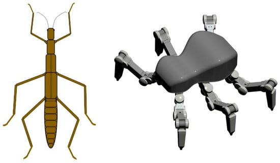
Figure 1.
Insect robot and hexapod robot HITCR-II.
Hexapod robot HITCR-II has 18 joints and complex movements. As shown in Figure 2, is the reference coordinate system based on the ground, and is the trunk coordinate system, the origin of which coincides with the geometric center of the trunk. The X, Y, and Z coordinate axes meet the right-hand helix law, the X axis is consistent with the forward direction of the robot, and the Z axis is perpendicular to the torso surface and opposite to the direction of gravity. The three left legs of the robot are represented by L1, L2, and L3 respectively, and the three right legs are represented by R1, R2, and R3, respectively. Starting from L1, the robot is arranged in a counterclockwise order. is the leg coordinate system.
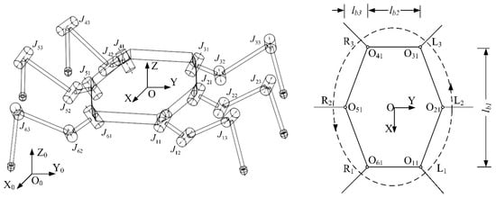
Figure 2.
The reference coordinate system and the trunk coordinate system.
In Figure 3, is the coordinate system of the n-th joint of the m-th leg. The coordinate axis is consistent with the direction of the joint axis, and the forward direction and the opposite direction of gravity are positive. The Ym-axis is connected to the lower joint of the joint. The axis of one limb coincides and points to the next joint. The foot end coordinate system is represented by , and its coordinate axis direction is consistent with .
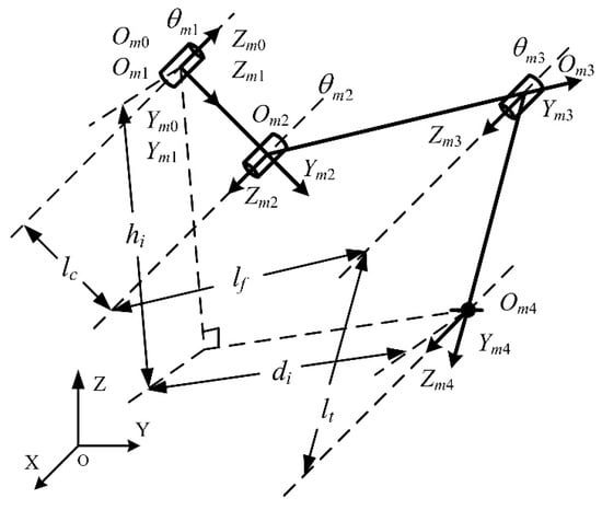
Figure 3.
Joint coordinates of legs.
The main parameters of the robot HITCR-II are shown in Table 1. The weight is 3.2 kg, the length and width of the trunk are 320 and 136–196 mm respectively, and the longitudinal and transverse spans under the initial pose are 400 and 380 mm, respectively. Compared with hexapod robots with the same performance at home and abroad, the robot has obvious advantages of miniaturization and lightness. In order to reduce the volume and weight of the joint, a joint design scheme based on brushless DC motor drive, harmonic reduction, and synchronous belt drive was developed. The final structural parameters of the realized joint are 58.5 mm long, 42 mm wide, 28 mm thick and 118 g heavy. The base joint angle range is , base-femoral joint angle is , and femoral-tibial joint angle is . Figure 4 is the structure of modularized joint.

Table 1.
The structure parameters of the robot.
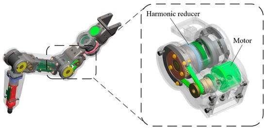
Figure 4.
The structure of modularized joint.
2. Adaptive Foot Trajectory Planning for Rugged Terrain
Foot trajectory planning solves the problem of generating the foot motion trajectory when a hexapod robot is walking. This planning meets the needs of the robot’s motion while constraining its motion according to its structure, motion, and dynamic characteristics to ensure that it moves in an orderly, stable manner. Aiming at the complex, rugged terrain, how to realize the adaptability of the foot trajectory to the terrain change, which can generate a continuous trajectory that can autonomously cross certain obstacles and find a stable foot point, is an important research issue.
2.1. Adaptive Strategy for Foot Trajectory Planning
The foot of the hexapod robot is composed of a base joint, a base-femoral joint, and a femoral-tibial joint. A reference coordinate system, , for trajectory planning is established with the center of the base joint axis as the coordinate origin to facilitate gait control, unified planning, and coordination of the trajectory of each leg and foot end. The direction of each axis of the coordinate system is consistent with the trunk coordinate system , is perpendicular to the trunk and opposite to gravity, and is the same as the forward velocity, V, of the robot. The model of the planned foot trajectory is shown in Figure 5. The swing phase and support phase in the foot trajectory are planned in the reference coordinate system . origin is the projection of the m-th leg and foot endpoint on the plane of the corresponding reference coordinate system in the initial pose. Track_A (curve QATBP) is the projection of the swing phase trajectory on the plane . The trajectory is divided into the ATB section of the guide layer and the adjustment layer CQ and BP. The trajectory of the guidance layer mainly realizes the swing function and has good shape and dynamic characteristics. This layer is divided into an upper guidance layer and a lower guidance layer. The distinction between the upper guidance layer and lower guidance layer is used for the robot’s autonomous judgment and selection of pose control strategies. The adjustment layer trajectory is mainly used to realize the adaptation function to the ground. It is divided into upper and lower adjustment layers, and a simple trajectory is used to solve the ups and downs of the foot directly and effectively. The judgment of the foot point needs to combine the force sensing function of the leg and use the joint torque sensor of the base-femoral joint to sense the contact of the foot end with the ground. Then, the foot end is converted from the swing phase trajectory to the support phase trajectory. When the robot is walking on a flat terrain, the swing phase trajectory only contains the guidance layer, starting at point A and ending at point B. When walking on a rugged terrain, the swing phase trajectory can end at any point of the curve TBP section to switch to the support phase trajectory. If the end point is higher than the horizontal position, it ends at the guide layer, and if it is lower than the horizontal position, it ends at the adjustment layer. Track_B (curve) is the trajectory of the swing leg entering the support phase in advance, and this trajectory meets the needs of gait control.
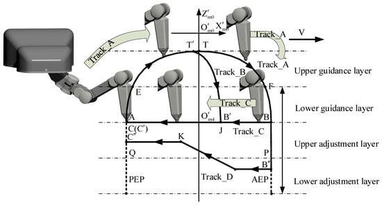
Figure 5.
Projection of foot-end trajectory model in the XOZ plane of the trunk coordinate system.
The coordination of the trajectory of each foot end of the supporting phase realizes the expected motion of the torso. The motion of the torso is planned in the ground reference coordinate system. The end of the foot in the supporting motion is stationary relative to the ground reference coordinate system without sliding. Thus, the motion of the torso can be converted. The trajectory of each foot end is separately planned for the movement of the end points of each supporting leg relative to the trunk coordinate system. Track_C (line BA) is the projection of the swing phase trajectory on plane X. When the hexapod robot simultaneously adjusts its pose during traveling, the trajectory is shown as Track_D (line ). The JK segment is the projection of the composite trajectory supporting the forward movement of the torso and the posture change. For foot trajectory based on the above strategic planning, in the case of mildly rugged terrain, while the foot trajectory adapts to the changing terrain, it can ensure that the trunk maintains the same posture based on the initial level of walking during the entire walking process. In severely rugged terrain under the circumstances, the torso can be more widely adapted to the changing terrain through the adjustment of the pose, and the constantly changing torso plane itself is used as the reference during the entire walking process to enable the robot to adapt to the gradual terrain (such as slopes, stairs) conditions.
2.2. Autonomous Terrain Judgment Strategy Based on Layer Identification of Tracking
The purpose of distinguishing terrain is to use different pose control strategies to help the robot cross the terrain. The adaptive trajectory planning strategy for rugged terrain divides the swing phase trajectory of the foot into an upper guidance layer, a lower guidance layer, an upper adjustment layer, and a lower adjustment layer. According to the robot structure parameters and walking needs, the height of each layer of the trajectory is specified to be 40 mm. The purpose of layer identification of tracking (LIT) is to determine the coordinate range of which layer of the trajectory is located in Z-axis coordinate of the leg coordinate system, of foot end point , and the interval of each layer is represented by and . In execution, the position of each foot end can be obtained by kinematic calculation based on the joint angular position sensing data in real time. The LIT autonomous judgment strategy is expressed as follows:
LT_State is the flag for lightly rugged terrain, HT_State is the flag for severely rugged terrain, and the status flag is 1 to stimulate the corresponding mode. When LT_State = 0 and HT_State = 0, it is judged as no foothold. As shown in Figure 6, in case (a), when the end of the foot swings from the reference ground to the terrain with a height range of [0,40] mm, ordinate of end point in the leg coordinate system is located in the lower guide layer, and the terrain is judged to be slightly rugged by leg i. In case (b), when the end of the foot swings from the reference ground to the terrain with a height range of [40,80] mm, ordinate of end point in the leg coordinate system is located in the upper guide layer, and the terrain is judged to be severely rugged by leg i. When the foothold is in the adjustment layer, the judgment is the same as that in the navigation layer. If any leg determines that the terrain is severely rugged terrain, the pose adjustment mode corresponding to the severely rugged terrain is stimulated.
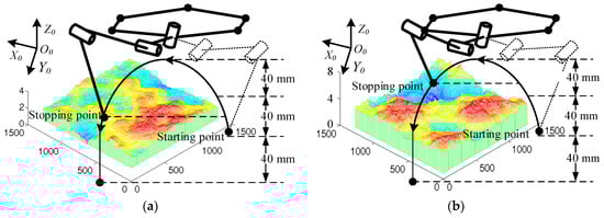
Figure 6.
Two diagrams of autonomous terrain identification strategy: (a) Identification of light rough terrain and (b) identification of high rough terrain.
Figure 7 shows the control scheme used by the hexapod robot to walk on rough terrain.
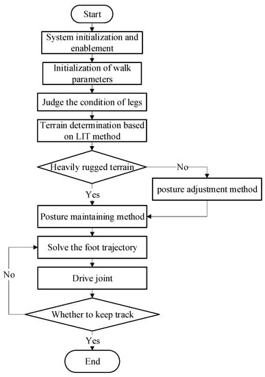
Figure 7.
The flow chart of single leg control.
3. Posture Maintenance Strategy for Mildly Rugged Terrain
The configuration and motion mode characteristics of the hexapod robot determine that it has a high stability margin. The stability of the walking robot is evaluated by the size of the stability margin (SM) (Zero Moment Point). The widely used criterion of the stability margin is the ZMP (Zero Moment Point) principle, which is defined as the minimum distance between the projection point of the center of gravity vector on the supporting polygon and each side of the polygon. The motion characteristics of the hexapod robot determine that it can be analyzed in a quasi-static way. Therefore, the minimum distance of the center of gravity from the supporting polygon to each side of the polygon is taken as the evaluation standard of the stability margin, ignoring the effect of inertia. As shown in Figure 8, the stability margin for n-side shape is shown as follows.
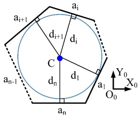
Figure 8.
Diagram of the stability margin.
The interference of mildly rugged terrain is not enough to cause its motion instability, but it will still affect the posture. Therefore, a posture maintenance strategy, which keeps the level and height of the torso unchanged based on the initial posture during walking, is proposed for mild ruggedness terrain. In order to obtain higher leg space, the hexapod robot was required to walk with TG (tripod gait) as the starting gait [29]. Adjust the position of the center of mass of the torso on the projection of the supporting polygon within the range of motion and take the minimum distance between the projection point and each side of the supporting polygon as the initial attitude of the hexapod robot. So, the initial level and height of the torso depends on the terrain.
3.1. Hexapod Robot Foot Force Distribution Model
The motion form of the hexapod robot is crawling. It can be analyzed as a quasi-static motion due to its low speed and stable motion. Analyzing the mechanical model of the robot aims to determine the relationship of the force between the supporting feet when the robot has a larger stability margin and use this foot force as feedback to control the position and attitude.
The mechanical model is shown in Figure 9. Global coordinate system is , and center of gravity is . The projection of the center of gravity on the torso coordinate system is located in the torso coordinate on the X axis, and it is close to origin O of the torso coordinate system because the robot configuration is symmetrically distributed with the geometric center in an elliptical shape in the initial pose. Taking the contact point between foot end of the i-th leg and the ground, external force received is , external moment is , and ground reaction force at the foot end of leg i is .
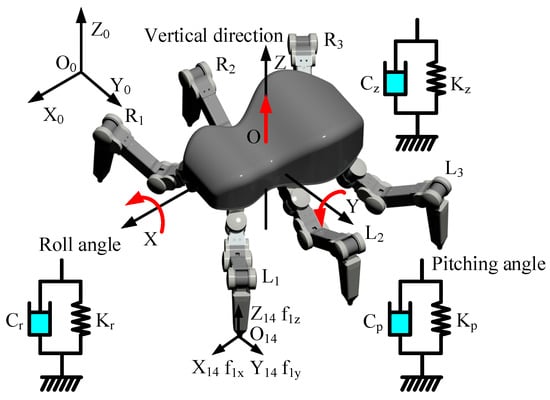
Figure 9.
Force equilibrium model of the hexapod robot.
The fluctuation of the robot in the vertical direction and the rotation along the pitch and roll directions are the main factors affecting its posture. These factors are related to vertical component of supporting leg foot end force . Therefore, the vertical component in . For straight component , pitch torque , and rollover torque in , the static balance model is obtained as follows:
Formula (1) is expressed in matrix form as follows:
The available full end force formula is as follows:
is pseudoinverse. When the robot is supported on three legs, no matter where the end of the foot is in any position corresponding to a certain state of the robot, the only solution for the size of the full force can be obtained by Formula (6). Under rugged terrain, the robot walks in a wave gait with more than three-leg support. At this time, if the foot force is solved according to this model, the system is indeterminate. Therefore, constraints must be added to make the system have a unique solution. When the supporting legs even bear the gravity of the robot, the robot has a large stability margin, a large carrying capacity, and a low energy consumption. Therefore, the minimum mean square error of the foot force is set as the objective function:
Among them, , where is the number of robot supporting legs. This can determine the foot end force in the initial posture.
3.2. Virtual Suspension Dynamic Model
3.2.1. Linear Model of Virtual Suspension Dynamic Model
According to the characteristics of the FBM mechanism of the hexapod robot, a virtual suspension dynamic model (VSDM) is established to suppress the change of posture during walking, in the vertical, pitch, and roll directions of the torso, as shown in Figure 3. A one-dimensional virtual spring damper is set up, and the vertical direction fluctuation and the pitch angle and roll angle disturbance are suppressed by controlling the spring damper. Here, the ground and the body are assumed rigid, and the mathematical expression obtained according to the model is as follows:
where , , and are the virtual spring stiffness coefficients in the vertical, pitch, and roll directions respectively, , , and are the virtual damping coefficient for vertical, pitch, and roll directions respectively, and are the moment of inertia in the pitch and roll directions respectively, z, , and are trunk height, pitch angle, and roll angle respectively, and is the robot weight.
After Equation (8), taking the Laplace transform, the characteristic equation of the virtual model in three directions is expressed as follows:
where , , and . The frequency characteristic equation is as follows:
The characteristic frequency and damping ratio of the system are expressed as follows:
The damping ratio is selected between 0.7 and 1.0 to improve the system response speed and reduce the overshoot. In addition, the interference caused by the pose control amount has a very low-frequency characteristic during the execution of the controller due to the collision and sliding of the foot with the ground and the change of the robot’s own motion state. The system’s characteristic frequency, , has a large value to avoid resonance. When the robot is in a static state, no disturbance is caused by the external and its own state changes. In this state, the corner frequency and damping ratio are = [240, 240, 60] and = [0.85, 0.85, 0.85], respectively. The mass of the robot is 3.2 kg, and the moments of inertia in the pitch and roll directions in the initial pose are respectively Substituting Ip = 8.98 × 10⁻² kg.m2 and Ir = 1.2 × 10⁻¹ kg.m2a into Formula (10), we can obtain Kz = 1.8 × 10⁴ N/m, Kp = 5.1 × 10³ Nm/rad, Kr = 6.7 × 10³ Nm/rad, Cz = 5.0 × 10² Ns/m, Cp = 3.7 × 101 Nms/rad, and Cr = 4.7 × 101 Nms/rad.
3.2.2. No Linear Model of Virtual Suspension Dynamic Model
When the robot is in a slow-motion state on a flat terrain, pose control can be realized by a linear time-invariant system determined by the Formula (8) model. However, when the robot is walking on rugged terrain, interference is caused by the change of its own state and the effect of the external environment on the body. The model in this case is expressed as follows:
where μz, , and are the control amounts of vertical, pitch, and roll directions respectively, , , and are the amounts of interference in the vertical, pitch, and roll directions respectively, and is the change of inertia in vertical, pitch, and roll directions.
The model includes changes in dynamic parameters caused by changes in the position of the center of gravity as well as the amount of interference introduced by the interaction between the foot and the ground. This model describes a nonlinear time-varying system, and the position tracking effect must be improved by controlling the position and velocity errors simultaneously to track the target pose better.
3.3. Two-Loop Sliding Mode Controller Based on VSDM Model
The unique synovial motion of the synovial membrane controller can make the system make small-amplitude, high-frequency reciprocating motion along the specified trajectory under certain characteristics. This motion can shield the influence of model parameters and external disturbances, so that the control system has good robustness. In order to realize the position and speed tracking control of the VSDM model, a sliding membrane controller with a double-loop structure is designed. As shown in Figure 10, the outer loop of the structure is a position loop, the inner loop is a speed loop, and the speed command output by the outer loop is used as the outer command of the inner loop.
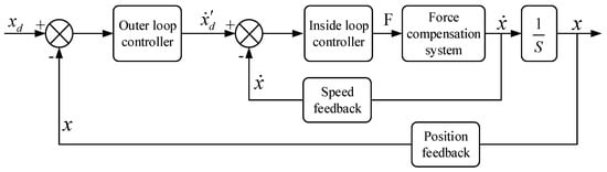
Figure 10.
Structure of a two-loop sliding mode control system.
The trunk height, pitch angle, and roll angle have the same mathematical model, so the same synovial controller can be used for control respectively, and the VSDM model can be further planned to obtain:
Force compensation amount is , and disturbance variable is , includes not only the amount of external interference, but also the amount of interference caused by the change of its own state.
4. Posture Maintenance Strategy for Heavy Rugged Terrain
4.1. Analysis of Pose Adjustment Strategy for Heavy Rugged Terrain
Compared with keeping the torso moving steadily in the initial posture under lightly rugged terrain, when walking on heavy rugged terrain, the robot needs to adjust the posture actively according to the changes in the terrain to adapt to the changing rugged terrain more widely and ensure the leg working space has good movement flexibility. For heavily rugged terrain, the robot adopts a posture adjustment strategy to adjust the height and inclination of the torso. As shown in Figure 11a, the pose of the robot represented red lines is analyzed in coordinate system based on the earth. The coordinates of the origin of the torso coordinate system in represent the position of the torso. When walking in complex terrain, the combined effect of posture adjustment and traveling motion makes the origin of the torso coordinate system move from to . In pose adjustment, facing convex terrain, a trunk height change amount is , and pitch angle change amount is ; facing recessed terrain, b trunk height adjustment amount is , and pitch angle adjustment amount is . Walking continuously changes the position of the torso coordinate system as the benchmark of motion planning through the adjustment of trunk height and inclination , then:
where and are the changes in the height and inclination of the torso during posture adjustment, and is the change in the height of the torso caused by the traveling motion during the non-posture adjustment. The movement of the robot is determined by the trajectory of the end of the foot. Traveling movement does not produce the change of the torso inclination because the trajectory of the end of the foot is planned in the torso coordinate system. and can approximately represent the change in altitude and slope of the current terrain from the initial horizontal plane, respectively. Pose adjustment achieves wide adaptability to gradual and rugged terrain through continuous adjustment of trunk height and inclination changes. Pose control has a clear distinction between light and severely rugged terrain. However, in practical applications, a type of terrain is slightly rugged in a certain walking cycle, while the overall observation during a period of travel is severely rugged. The analysis of this type of terrain is shown in Figure 11b.The blue lines represent the foot track of the robot.
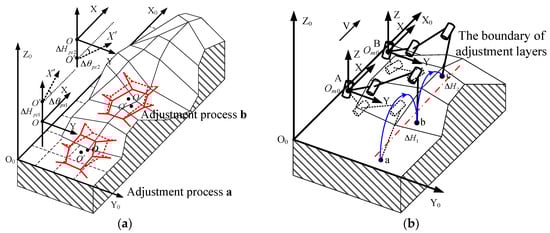
Figure 11.
The process of adjusting the pose on severe rugged terrain: (a) Analysis of terrain adaption mechanism and (b) analysis of pseudo-light rough terrain.
When the origin of the leg coordinate system is at point A, the end of the foot swings from position a to position b, and the end point of the foot end is located in the lower guide layer of the trajectory. Thus, the terrain is judged to be slightly rugged, and the posture maintenance strategy is stimulated. From the rugged terrain adaptive foot trajectory planning this article, the end position of the foot end on the trajectory of this cycle is the starting position of the next cycle. When the foot end swings again from position b to position c, the termination point is at the upper adjustment layer, and the terrain is determined to be heavily rugged. The behavior can be expressed as follows:
where is the height of the end point of the foot end of the first cycle relative to the start point, is the height of the end point of the foot end of the second cycle relative to the start point, is the height of the guide layer under the trajectory, and is the height of the track guide layer.
In general, the accumulation of changes in the trajectory height in multiple cycles can be expressed as follows:
where is the height amount of the end point of the foot end of the i-th cycle relative to the start point.
For the sag terrain, the same conclusion can be obtained by analyzing the problem in the adjustment layer. The above analysis shows that for pseudo-lightly rugged terrain, the LIT strategy has a cumulative effect, and a reasonable pose control strategy can be invoked by accurately identifying the terrain.
4.2. Posture Adjustment Strategy Based on Master Polygon
4.2.1. Master Polygon
The polygon formed by the end points of each supporting foot of the hexapod robot in the torso coordinate system is called the configuration polygon (CP). Affected by the rugged terrain, the CP is generally a spatial polygon. Figure 12 shows the CPs formed by the end points of the feet when supported by three, four, and five legs. In the case of four and five legs, not all the end points of the feet are on the same plane. From the gait rules, at least three non-adjacent legs are in the supporting phase at any time, and the triangle that is stipulated to be formed by connecting the end points of the three non-adjacent legs is the master polygon (MP). A unique MP always exists in any CP during walking, or it is the LMP formed by the end of the foot of leg , , and , or the RMP formed by the end of the foot of leg , , and . The CP of the hexapod robot and the terrain jointly determine its pose, and it cannot be used as a reference plane to measure the pose of the torso because it is a spatial polygon, while MP approximates the orientation characteristics of the CP, so MP is used as the position. The reference plane for pose adjustment and the selection rules are as follows:
where and are the status flags of the leg support, and are the status flags of LMP and RMP respectively, and the priority of LMP is higher than that of RMP.
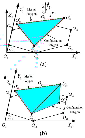
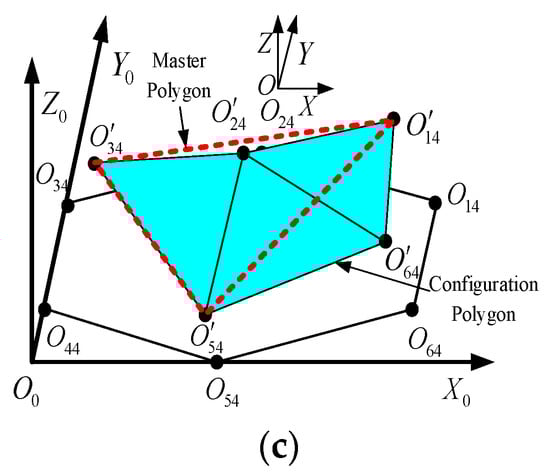
Figure 12.
Analysis of main support polygon: (a) Configuration polygon with three stance legs, identification of light rough terrain, (b) configuration polygon with four stance legs, and (c) configuration polygon with five stance legs.
4.2.2. Posture Adjustment Method Based on the CP
After the MP is determined, the posture of the torso is adjusted by taking the line of the coordinate origin of the hind leg and the middle leg of the main support leg as the reference axis, and the torso plane parallel to the MP as the control target. As shown in Figure 13a, taking the six-leg simultaneous support state as an example, leg triggers severely rugged flag , and it is judged as LMP. The reference axis is , and the posture control target is plane parallel to the LMP. The control quantity composed of the height of the trunk, the pitch angle, and the roll angle can then be obtained. In pose adjustment, except for the two legs that determine the reference axis, the trajectories generated by the pose adjustment movement at the origin of the other leg coordinate systems are shown as , , , and , as shown in Figure 13b, where the foot end trajectory is planned in the leg coordinate system. The trajectory is an arc with the same shape and opposite direction as the origin of the leg coordinate due to the relative motion because the supporting foot end is stationary relative to the ground. In pose adjustment under this planning method, the pitch angle and the yaw angle have a strict correspondence because of the height of the trunk. Therefore, only one of the factors, instead of three, is required as the control quantity to realize the pose adjustment. The amount is controlled separately, reducing the control burden.
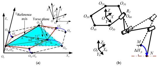
Figure 13.
Posture adjusting mode: (a) Trunk-adjusting mode, and (b) leg-adjusting mode identification of high rough terrain.
The hexapod robot divided the terrain into mild rugged terrain and severe rugged terrain through the LIT strategy and adopted the corresponding pose control strategy, respectively. After foot trajectory compensation, the foot state and trajectory were adjusted, and the foot trajectory was re-planned. Figure 14 shows the control process of the hexapod robot when it crosses rugged terrain.
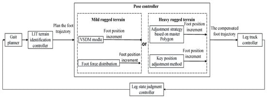
Figure 14.
The control process diagram when the hexapod robot crosses rugged terrain.
5. Simulation and Experiment
5.1. Posture Control Simulation for Uneven Terrain
As shown in Figure 15a, the terrain is randomly generated in a three-dimensional (3D) coordinate system by using MATLAB software, and the maximum height difference of the entire terrain is 210 mm. In addition, the hexapod robot model is established to verify whether the posture control strategy can realize the robot’s traversing of rugged terrain. The target path of the robot traversing the terrain is a diagonal line through the coordinate origin, and different colors of the terrain represent different heights. The projection of the main support foot in the XY plane in each stage of walking is calculated, as shown in Figure 15b, where the dotted line is LMP projection and the solid line is RMP projection. Finally, the robot successfully traverses the terrain.
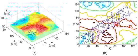
Figure 15.
Posture control simulation in MATLAB: (a) Simulation environment of unstructured terrain walking, and (b) projection on the XY plane of MP.
Figure 16 shows the curves of the trunk yaw angle, pitch angle, and roll angle. Each curve either maintains a zero value or changes smoothly and slowly at different stages. This control method can make the robot switch between mild and severe rough posture control mode in a timely manner with the change of terrain. In addition, it can adapt to the changing rugged terrain and complete the walking of the complex terrain through the posture adjustment of severe rough terrain.
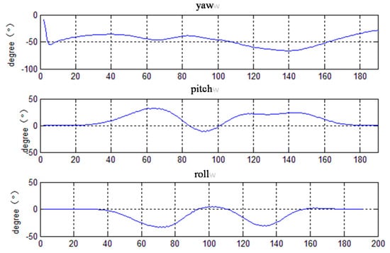
Figure 16.
Curve of angles of posture.
Figure 17 is the foot trajectory curve that the hexapod robot adjusts automatically when encountering obstacles. The trajectory at the beginning is planned according to the established boundary conditions and functions. Starting from the starting point A, the foot touches the obstacle during the swing process and ends. For the initial swing trajectory, update the boundary conditions and call the support phase trajectory function. Starting from the transition point B, the foot end moves along the support phase trajectory to the end point C. It can be seen that this strategy can generate a foot trajectory that satisfies the functions of swinging and supporting motion and enables the trajectory to be adjusted autonomously in real time according to changes in terrain [30].
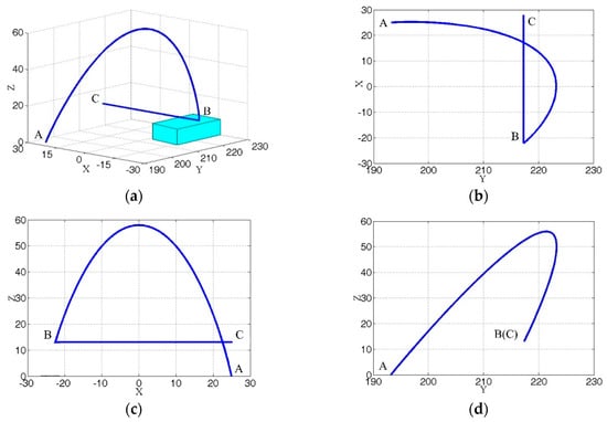
Figure 17.
Foot trajectory simulation in MATLAB: (a) Adaptive foot-end trajectory in a cycle, (b) projection of trajectory in XY, (c) projection of trajectory in the XZ plane, and (d) projection of trajectory in the YZ plane [29].
5.2. Posture Control Experiment on Unstructured Terrain
The purpose of the posture control experiment is to verify the ability of the hexapod robot HITCR to traverse complex terrain under the control of the posture controller and the effect of the gravity center position control method based on foot end force distribution on improving walking stability. The terrain is planned to analyze the effects of the slightly rugged terrain posture maintenance and the severely rugged terrain posture adjustment, as shown in Figure 18. The terrain is divided into three parts: flat, lightly rugged, and heavily rugged. The rugged terrain is paved with angular gravel and stones of different sizes and roughness, and the protruding terrain is piled up in the severely rugged part. The maximum height of the protruding relatively flat terrain is about 210 mm.
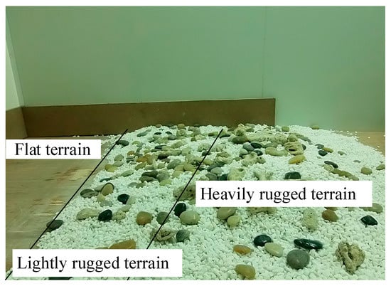
Figure 18.
Staged unstructured terrain.
Figure 19 shows the process screenshot of the robot crossing the terrain. As shown in (a), the robot enters the slightly rugged terrain after two walking cycles, and the maximum obstacle height of the terrain is less than 40 mm, so the posture maintenance strategy is selected. As shown in (c), the robot enters the heavily rugged terrain after another 12 walking cycles, and in (d) the foot falls on a stone with a height of about 50 mm. This behavior can stimulate the posture adjustment strategy of the severely rugged terrain. The robot climbs the convex terrain in (e) and finally crosses the complex terrain in (f). Therefore, the experimental results verify the effectiveness of the posture controller and the walking ability of the HITCR in rough terrain.
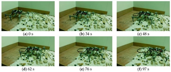
Figure 19.
Posture control experiment on staged unstructured terrain.
The observed values of pitch angle and roll angle are shown in Figure 20a,b, respectively. Under the two conditions, the robot can successfully cross the staged unstructured terrain through the posture maintaining strategy and the posture adjustment strategy and adjust the posture of the trunk according to the changes of the terrain in the severe rough stage. The results show that the pitch angle and roll angle have a smooth, small fluctuation under the condition of the posture controller based on the VSDM model, but the pitch angle and roll angle have a large fluctuation under the condition of no posture controller based on the VSDM model. The effect of keeping the trunk horizontal in mild rough terrain is poor. The maximum angle offsets of pitch angle and roll angle are 5.2° and 4.9°, respectively. The posture controller based on the VSDM model is like a low-pass filter, which can filter out external environment interference and unstable factors of the robot’s own motion and improve the stability of the motion on the basis of realizing the target motion.
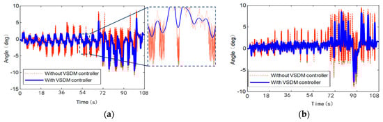
Figure 20.
The observed values of pitch angle and roll angle: (a) Curve of pitch angle, and (b) curve of roll angle.
5.3. Climbing Experiment on Stepped Terrain
The ladder is a typical discontinuous gradual terrain, which belongs to the same gradient terrain as the slope terrain. The climbing ability of this kind of terrain enables the robot to adapt to the terrain more widely. The ladder climbing movement requires the robot to have strong movement ability, and it needs to adapt to the discontinuous changes of the terrain through continuous posture adjustment compared with the slope terrain.
As shown in Figure 21, the heights of the three steps are 51, 34, and 51 mm from the bottom to the top. The step size of the robot is 50 mm, and the maximum height of the foot track is 80 mm. During climbing, the robot’s motion is stable. Every time a leg moves from swing phase to support phase, the posture of the trunk is adjusted to adapt to the changing step terrain. Finally, the robot successfully climbs to the top of the ladder terrain.
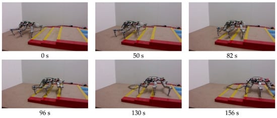
Figure 21.
Process of stair climbing.
The curves of pitch angle and roll angle observed in climbing the ladder are shown in Figure 22a,b, respectively. The pitch angle starts from point zero and adjusts according to the change of step height. The maximum value is 11°, and the pitch angle returns to zero after the robot climbs to the top completely. The roll angle starts from point zero and changes with the change of terrain and the replacement of leg motion state, and the maximum offset is 3.2°. After the robot fully climbs to the top, the pitch angle returns to zero. The autonomous terrain identification method based on the LIT, mild rugged posture maintenance strategy, and severe rugged posture adjustment strategy can autonomously identify the changed step terrain and adopt the corresponding posture control strategy to make the robot successfully climb the ladder terrain. In addition, the curves of pitch angle and roll angle are smooth, and the motion of posture adjustment is stable.
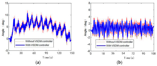
Figure 22.
The curves of pitch angle and roll angle observed in climbing the ladder: (a) Pitch angle in stair climbing, and (b) roll angle in stair climbing.
6. Conclusions
This paper proposed a rugged terrain adaptive strategy based on foot trajectory to solve the problem of hexapod robot posture control in the unstructured terrain climbing. The unstructured terrain was judged as mild unstructured and severe unstructured, and the corresponding posture adjustment mode was activated by combining the change of foot trajectory and the autonomous terrain judgment strategy based on LIT. A VSDM was established to keep the trunk moving smoothly based on the initial posture and reduce the influence of mild unstructured terrain on posture changes. In severe unstructured terrain, the hexapod robot actively adjusts the height and inclination of the trunk and uses the main support triangle MP formed by the support foot as the reference plane for posture adjustment. According to the MP projection in the MATLAB simulation experiment, when the robot passes through rugged ground, the variation curve of trunk yaw angle, pitch angle, and roll angle will either maintain a zero value or change smoothly and slowly at different stages, and the robot can switch between mild and severe unstructured posture control mode in a timely manner. The experiments show that the posture controller based on the VSDM model can filter out the disturbance of external environment and unstable factors of the robot’s own motion. In addition, the robot can autonomously identify the changing stair terrain and adopt the corresponding posture control strategy to make it successfully complete the stair climbing.
The innovation of the posture adjustment strategy for uneven terrain in this paper is as follows: First, the hexapod robot can automatically divide the climbing terrain into mild uneven terrain and severe uneven terrain according to the foot motion trajectory, and accurately activate the corresponding posture adjustment strategy according to the terrain. Second, the hexapod robot adjusts its posture according to the VSDM model for flat and mild uneven terrain. In severe uneven terrain, the robot needs to adjust one of the trunk’s height, pitch angle, and deflection angle based on the main support triangle MP. Under the premise of ensuring the robot’s climbing ability, the hybrid use of the two posture adjustment strategies improves the passing efficiency. Third, the simulation and experimental results show that the control method can switch the posture control mode in a timely manner. The posture controller based on the VSDM model can filter out the external environment disturbance and unstable factors of the robot’s own motion and improve the stability of the motion on the basis of realizing the target motion. This control method has good adaptability and passing performance to unstructured terrain.
The experimental results showed that the VSDM controller can filter out small vibrations during the adjustment of the pose, but the smoothness of the adjustment needs to be further enhanced. When the robot travels heavy rugged terrain, the degree of torso vibration was more than when traversing lightly rugged terrain. The posture adjustment control algorithm and controller used in the heavy rugged walking need to be optimized. In view of the above problems, the hexapod robot needs to be studied in depth from the following aspects: First, the hexapod robot needs to redesign and optimize the controller to improve the control accuracy, response speed, and stability of the torso during the adjustment process. Second, improve the accuracy and speed of robot attitude adjustment for heavy rugged terrain. Third, more external interference should be added in subsequent experiments to verify the adaptability of the robot in a complex environment.
Author Contributions
Y.L. built the dynamic model of the hexapod robot, contributed to the mathematical model, and was responsible for the experiments. C.W. contributed to the program design of the pose controller and wrote the paper. H.Z. developed and came up with ideas about the pose control method for the hexapod robot. J.Z. oversaw and advised the research. All authors have read and agreed to the published version of the manuscript.
Funding
This work was supported by the National Key R&D Program of China (Grant No. 2018YFB1307602), open foundation of the State Key Laboratory of Robotics and Systems (Harbin Institute of Technology) under grant No. SKLRS201816B, Major Research Plan of the National Natural Science Foundation of China (Grant No. 91648201), and Foundation for Innovation Research Groups (Grant No.51521003) of the National Natural Science Foundation of China. This research received no external funding.
Conflicts of Interest
The authors declare no conflict of interest.
References
- Maufroy, C.; Kimura, H.; Takase, K. Integration of posture and rhythmic motion controls in quadrupedal dynamic walking using phase modulations based on leg loading/unloading. Auton. Robot. 2010, 28, 331–353. [Google Scholar]
- Theeravithayangkura, C.; Takubo, T.; Ohara, K.; Mae, Y.; Arai, T. Adaptive Gait for Dynamic Rotational Walking Motion on Unknown Non-Planar Terrain by Limb Mechanism Robot ASTERISK. J. Robot. Mechatron. 2013, 25, 172–182. [Google Scholar]
- Celaya, E.; Porta, J.M. A control structure for the locomotion of a legged robot on difficult terrain. IEEE Robot. Autom. Mag. 1998, 5, 43–51. [Google Scholar]
- Wang, Z.; Ding, X.; Rovetta, A.; Giusti, A. Mobility analysis of the typical gait of a radial symmetrical six-legged robot. Mechatronics 2011, 21, 1133–1146. [Google Scholar]
- Zhang, L.; Wang, F.; Gao, Z.; Gao, S.; Li, C. Research on the Stationarity of Hexapod Robot Posture Adjustment. Sensors 2020, 20, 2859. [Google Scholar]
- Chen, G.; Jin, B.; Chen, Y. Nonsingular fast terminal sliding mode posture control for six-legged walking robots with redundant actuation. Mechatronics 2018, 50, 1–15. [Google Scholar]
- Hu, N.; Li, S.; Zhu, Y.; Gao, F. Constrained model predictive control for a hexapod robot walking on irregular terrain. J. Intell. Robot. Syst. 2019, 94, 179–201. [Google Scholar]
- Wu, X.; Li, Y.; Consi, T.R. Posture Synthesis and Control of a Symmetric Hexapod Robot on Corrugated Surfaces for Underwater Observation. In Proceedings of the ASME International Mechanical Engineering Congress and Exposition, Seattle, WA, USA, 11–15 November 2007; Volume 43033, pp. 1265–1274. [Google Scholar]
- Song, S.M.; Waldron, K.J. Machines That Walk: The Adaptive Suspension Vehicle; MIT Press: Cambridge, MA, USA, 1989. [Google Scholar]
- Bjelonic, M.; Kottege, N.; Beckerle, P. Proprioceptive control of an over-actuated hexapod robot in unstructured terrain. In Proceedings of the 2016 IEEE/RSJ International Conference on Intelligent Robots and Systems (IROS), Daejeon, Korea, 9–14 October 2016; pp. 2042–2049. [Google Scholar]
- Chen, C.; Guo, W.; Zheng, P.; Zha, F.; Wang, X.; Jiang, Z. Stable Motion Control Scheme Based on Foot-Force Distribution for a Large-Scale Hexapod Robot. In Proceedings of the 2019 IEEE 4th International Conference on Advanced Robotics and Mechatronics (ICARM), Toyonaka, Japan, 3–5 July 2019; pp. 763–768. [Google Scholar]
- Yoneda, K.; Iiyama, H.; Hirose, S. Sky-hook suspension control of a quadruped walking vehicle. J. Robot. Soc. Jpn. 1994, 12, 1066–1071. [Google Scholar]
- Khan, S.G.; Herrmann, G.; Pipe, T.; Melhuish, C.; Spiers, A. Safe adaptive compliance control of a humanoid robotic arm with anti-windup compensation and posture control. Int. J. Soc. Robot. 2010, 2, 305–319. [Google Scholar]
- Wang, W.J.; Chou, H.G.; Chen, Y.J.; Lu, R.C. Fuzzy control strategy for a hexapod robot walking on an incline. Int. J. Fuzzy Syst. 2017, 19, 1703–1717. [Google Scholar]
- Huang, Q.J.; Nonami, K. Humanitarian mine detecting six-legged walking robot and hybrid neuro walking control with position/force control. Mechatronics 2003, 13, 773–790. [Google Scholar] [CrossRef]
- Buchanan, R.; Bandyopadhyay, T.; Bjelonic, M.; Wellhausen, L.; Hutter, M.; Kottege, N. Walking posture adaptation for legged robot navigation in confined spaces. IEEE Robot. Autom. Lett. 2019, 4, 2148–2155. [Google Scholar] [CrossRef]
- Liu, Y.; Gao, H.; Ding, L.; Liu, G.; Deng, Z.; Li, N. State estimation of a heavy-duty hexapod robot with passive compliant ankles based on the leg kinematics and IMU data fusion. J. Mech. Sci. Technol. 2018, 32, 3885–3897. [Google Scholar] [CrossRef]
- Tikam, M.; Withey, D.; Theron, N.J. Standing posture control for a low-cost commercially available hexapod robot. In Proceedings of the 2017 IEEE/RSJ International Conference on Intelligent Robots and Systems (IROS), Vancouver, BC, Canada, 24–28 September 2017; pp. 3379–3385. [Google Scholar]
- Nelson, G.M.; Quinn, R.D. Posture control of a cockroach-like robot. IEEE Control Syst. Mag. 1999, 19, 9–14. [Google Scholar]
- Orin, D.E.; Oh, S.Y. Control of Force Distribution in Robotic Mechanism Containing Closed Kinematic Chains. Trans. ASME, J. Dyn. Syst. Meas. Control 1981, 102, 134–141. [Google Scholar] [CrossRef]
- Klein, C.A.; Kittivatcharapong, S. Optimal force distribution for the legs of a walking machine with friction cone constraints. IEEE Trans. Robot. Autom. 1990, 6, 73–85. [Google Scholar] [CrossRef]
- Nahon, M.A.; Angeles, J. Optimization of Dynamic Forces in Mechanical Hands. Trans. ASME J. Mech. Des. 1991, 113, 167–173. [Google Scholar] [CrossRef]
- Chen, X.; Watanabe, K. Optimal force distribution for legs of quadruped robot. Mach. Intell. Robot. Control 1999, 1, 87–94. [Google Scholar]
- Waldron, K. Force and motion management in legged locomotion. IEEE J. Robot. Autom. 1986, 2, 214–220. [Google Scholar] [CrossRef]
- Galvez, J.A.; Estremera, J.; De Santos, P.G. A new legged-robot configuration for research in force distribution. Mechatronics 2003, 13, 907–932. [Google Scholar] [CrossRef]
- Vidoni, R.; Gasparetto, A. Gasparetto. Efficient force distribution and leg posture for a bio-inspired spider robot. Robot. Auton. Syst. 2011, 59, 142–150. [Google Scholar] [CrossRef]
- Liu, Y.; Ding, L.; Gao, H.; Liu, G.; Deng, Z.; Yu, H. Efficient force distribution algorithm for hexapod robot walking on uneven terrain. In Proceedings of the 2016 IEEE International Conference on Robotics and Biomimetics (ROBIO), Qingdao, China, 3–7 December 2016; pp. 432–437. [Google Scholar]
- Mahapatra, A.; Roy, S.S.; Pratihar, D.K. Study on feet forces’ distributions, energy consumption and dynamic stability measure of hexapod robot during crab walking. Appl. Math. Model. 2019, 65, 717–744. [Google Scholar] [CrossRef]
- Zhang, H.; Liu, Y.; Zhao, J.; Chen, J.; Yan, J. Development of a bionic hexapod robot for walking on unstructured terrain. J. Bionic Eng. 2014, 11, 176–187. [Google Scholar] [CrossRef]
- Zhang, H.; Wu, R.; Li, C.; Zang, X.; Zhu, Y.; Jin, H.; Zhang, X.; Zhao, J. Adaptive motion planning for HITCR-II hexapod robot. J. Mech. Med. Biol. 2017, 17, 1740040. [Google Scholar] [CrossRef]
© 2020 by the authors. Licensee MDPI, Basel, Switzerland. This article is an open access article distributed under the terms and conditions of the Creative Commons Attribution (CC BY) license (http://creativecommons.org/licenses/by/4.0/).