1. Introduction
The deployment of UWSNs (Underwater Sensor Networks) requires a large number of tools and sensors which are located in a specific area for monitoring. According to [
1], due to sea currents, the movement at underwater sensor networks is usually 2–3 m/s. So, it is required great attention from the designer in order to apply data communication techniques and protocols as efficiently as possible. The acoustic waves are widely used in underwater communication systems due to their low absorption in aquatic environments, where radio or optical waves cannot sufficiently propagate [
2]. The ocean sea can be generally divided into shallow area and deep zone, whose basic distinguishing features are generally [
1]:
- -
depth (0–100 m for the shallow area and up to 10 km for deep area),
- -
temperature (at shallow areas may have fluctuations and assumes usually relatively high values, while in very deep areas it reaches constant low value),
- -
scattering factor (cylindrical for shallow and spherical for deep areas).
The shallow areas greatly influence the acoustic channel due to its large gradient temperature, salinity variations and the effect of multipath due to surface and bottom reflections.
All these variations bring changes in the network that can be used to monitor. There are various survey studies that give a full detail report about the available methodologies for the channel utilization, impact of environment factors, localization of nodes, routing protocols and the effect of packet size on communication [
1]. While others are focused on the estimation of simulation tools and testbeds [
3], as their implementation is still expensive. An accurate simulation model for sure can help to create an approximation of the behavior of UWSNs in a real scenario. This helps to highlight new directions of research for further improvement in UWSNs.
That is why we have simulated different distribution of link failures for DEADS (Depth and Energy Aware Dominating Set Based Algorithm) routing algorithm at [
4]. It is important to find out how missing links will influence the network lifetime and residual energy of network, because the right chosen of node degree can help specially when the energy of network is going down. Another physical element that influences the node degree, is the mobility of the nodes [
5]. There are compared two different kinds of networks: one with settled positioning of the nodes from the beginning of the simulation and the other where the nodes change their position during the simulation. In the second case, the distances change any time, nodes move to different random positions and the network is on a continuous change of topology and nodes role. Due to the harsh environment, the conditions of network are not stable, that is why again is estimated also the presence of link failures. The results bring to the conclusion that where the nodes move due to water flow then node degree can diminish with time, that means that the network is less connected. The energy also in this case still is less because few nodes are active. This study helps to have the results of the network that keeps changing and shows the results of the calculated residual energy in the network, that is very important for the lifetime of a network that needs to monitor such difficult environment.
After that we studied the impact of intermittent noises in the range of acoustic modem communication [
6]. As we saw intermittent noises, when presented they have a significant impact on decreasing the transmission range. The calculations made for the parameters of the modem Evologics S2 CR7/17 showed that for the oceanic environment with the minimum received noise level, the range of communication is depending on the frequency from 9634 m to 4286 m, or on average 6414 m. Our calculations for the impact of intermittent noise showed that this transmission range may, in certain conditions, decrease considerably. According to Knudsen’s lines, we calculated the maximum relative distances that this modem is capable to transmit. So, the transmission range for speeds of 5, 10, 20, and 30 knots of wind at the average bandwidth of the communication band dropped to 4218, 2947, 1804, and 1083 m respectively. There is a noticeable decreasing of the communication range compared to the noise level when we have a zero-speed velocity, the average value of which is 6414 m. At the 30 knots speed the communication radius is only one-sixth of this value. So, future designers of these networks should seriously consider the effect of wind noise, because 30 knot speed is not the highest possible wind speed in the oceans. Franz’s theoretical predictions for noise levels based on rain’s resistance is used to calculate the respective transmission range. The calculations for 0.1, 1 and 4 inches, give the respective average transmission range 1912, 595 and 203 m.
Furthermore, we analyzed the case of seismic activity and biological noises. In the case of noise as a consequence of seismic activity, the average transmission range was 641, while in the case of shrimps was 265 m. So, these noises also have a significant impact on the acoustic underwater networks. The main conclusion of the study was the indisputable need that future designers of UWSN might consider the impact of intermittent noise. These noises are not always present in the ocean environment, but can influence a lot the network, for example, seismic activity, when a real-time transmission is needed. Our assessment is that in these networks is possible a very accurate transmission of information under normal conditions. We estimated that a noise signal ratio of 18.46 dB and with a transmission probability of 70% of the 4000 bit packet, is enough. Comparing this with the acoustic transmission power, which was 175.8 dB, the target SNR (Signal-to-Noise Ratio) ratio is low, enabling accurate transmission of large-range information. If appropriate measures are taken to deal with intermittent noises, UWSN can be very accurate in transmitting information.
While in this paper, we present an improved algorithm of DEADS, that can be applied in many underwater environments and coastal areas with variation of salinity and temperature within a range of concrete values. The proposed solution is improving the transmission of the data generated by the sensing elements that will help measuring the capacity of the network in the shallow waters. The aim of the work is therefore to demonstrate the algorithm’s performance, developed in a prototype way and tested with simulation, in a real scenario. Throughout this study are considered shallow underwater areas, i.e., those areas in which the network of sensor nodes for monitoring does not exceed 200 m depth. UWSN in these areas are mainly set up for purposes such as water surveillance, pollution detection for rivers and seas, defense during military attacks, monitoring, disaster prevention, underwater minerals extraction, ocean data compilation or commercial use. So, to simulate a network of nodes in shallow areas, the main features and problems of these areas must be taken into account.
The remainder of the paper is organized as follows.
Section 2 deals with features of underwater capacity, especially to the propagation of acoustic signal. An extended mathematical model including any parameters associated with the transmission channel signal, propagation along the path of acoustic communication and underwater main noises are presented at the
Section 3. Formulas for SNR, acoustic channel capacity, underwater features related to multipath including loss due to reflections and some geo-acoustic properties for typical materials at the oceans bottom are also provided. The
Section 4 shows the simulations of environmental/reflection effects as well as network behavior and performance metrics taken into account after using the modified algorithm.
Section 5 presents the results of simulation as a function of salinity and temperature, and in presence of multi path.
Section 6 discusses the results while, finally, the Conclusions ends this paper.
2. Acoustic Channel
Designing an efficient acoustic channel is a challenge because of its underwater environment characteristics as stated, like multipath propagation which causes a signal power drop and phase oscillation. The Doppler effect is also another problem that is observed when there is a relative displacement of the sending and receiving nodes. The sound propagation speed and underwater noise are also considered to be taken into account, since they are factors which affect the performance of the acoustic channel [
6].
Capacity analysis and studies have been done for the channel and its dependence on the depth and temperature by considering losses as a result of dispersion and environment noise. The absorption rate estimation for the acoustic communication path is a function of the distance (between a pair of nodes) and the communication frequency used. The acoustic channel bandwidth increases with the increase of depth value and temperature and decreases by increasing the distance between the two nodes. A comparison between two methods used to determine the absorption coefficient is shown in literature, the first one by Thorp [
7], while the latter is by Fisher-Simons [
8]. While Thorp’s model considers a fixed value for depth and temperature (it does not consider changes in depth or temperature) for the calculation of acoustic channel capacity, instead the Fisher-Simons model takes into account the changes of these. In [
8], it has been shown that the channel capacity and throughput increase with the increasing of temperature value and depth, in the case of small communication distances. The authors also explain that the nodes positioned in ocean deep areas achieve high speed and throughput. According to the results obtained in [
8], a higher channel capacity would be possible if the same transmission power was maintained but with an increase of depth value. This result can be used in the design of adaptive transmission schemes for underwater mobile networks, or for the various power management methods that reduce transmission power to achieve a constant target bit rate with increasing depth. As a consequence of the bandwidth dependency from the transmission distance, we will get a high throughput only with multi-hop communication used and where messages are routed to some intermediate nodes. This is a desired feature to have in case of live streaming when using a single hop (great distance). In the analysis done in [
9], regarding the physical model of the acoustic channel by taking into account losses due to spread and environment conditions, Stojanovic has determined the bandwidth dependency from distance. Underwater acoustic channels suffer from attenuation of the signal along the acoustic communication path which depends not only on the space between the nodes but also on the signal frequency used.
A variation of the signal frequency is considered to calculate the losses due to signal absorption rate for the communication, which occurs due to the conversion of the acoustic power in high temperature. A shorter communication link provides more bandwidth compared to a longer link in an acoustic system. Therefore, its use brings an increase in the throughput of received information, and more efficient usage of the acoustic channel, but as well as consuming even less energy. A significant error rate per velocity of data transmission and high delays are problematic features for the acoustic channel. In [
10] several different techniques are compared in order to avoid different problems mentioned like the package size adaptation or forward error correction. Taking into account all these challenges related to underwater environments, there are required different methodologies to achieve a better usage of the acoustic channel, and this is of great interest for numerous researcher group, some of those that are useful for this study, will be mentioned in the following section.
3. Methodology
A scenario of underwater data transmission includes transmission nodes and receiver nodes. The communication links of underwater data are characterized by low rates of data transmission; this is mainly because of communication limitations due to the high propagation delays or low bandwidth. The effects of these limitations can be reduced by communicating in shorter distances and by using multi-hop communication for covering longer distances [
10]. The propagation of the acoustic signal is affected by the following channel parameters: transmitter signal power (source level, SL), the attenuation through the path of acoustic communication (path loss, PL), underwater noises (noise level, NL) and the multipath and Doppler effects [
11].
Table 1 [
12] shows the typical seabed materials and their properties, which play an important role in the multipath effect.
In our study Equation (1) is used to calculate the transmitter’s acoustic signal level [
11].
where
is the power at transmitter,
is the efficiency factor that considers the losses associated with the electrical to acoustic conversion,
is the projector directivity index. For the calculation of the path loss it is used Urick’s model [
13]. As presented in [
9,
14] the absorption that occurs in an underwater communication channel is given by:
where
is the distance (m), and
the frequency of the signal (kHz),
is the spreading factor and
is the absorption coefficient. The acoustic path loss can be expressed in dB as the sum of spreading loss and absorption loss by:
The spreading factor
describes the geometry of the acoustic signal propagation. The commonly used values of the spreading factor are
for the spherical spreading,
for the cylindrical spreading, and
for the practical spreading. The absorption coefficient (
) is calculate by using the Francois and Garrison formula [
5] which depends on frequency, pressure (depth), temperature, salinity, pH and the acoustic propagation velocity, as follows:
where the dependence on the pressure (depth) is given by
,
,
and the relaxation frequencies of Boric acid and (MgSO4) molecules are given by
and
. The effects of temperature are given by the coefficients
,
,
. The first term is related to the contribution of the boric acid (B(OH)
3), the second term due to the contribution of magnesium sulfate (MgSO
4) and the third due the contribution of pure water. All the coefficients of Equation (4) are calculated according to [
7,
15]. While to calculate the velocity of sound propagation the formula given by Medwin [
4] is used:
where
is the temperature (°C),
is the salinity (‰) and
the depth (m). An accurate model of underwater noise is required in order to determine the receiver’s SNR. There are three main contributors in the total underwater noise: ambient noise, self-noise and the intermittent noise. The ambient noise is the most well-defined noise. As stated by [
16], the ambient noise in the ocean can be modelled by using four sources: turbulence, shipping, waves, and thermal noise, calculated by the following empirical formulas:
where
is the shipping activity factor (
) and
is the wind speed (m/s). The main influencer, among these four sources are the wind-driven waves that contribute in frequencies from 100 Hz to 100 kHz.
The total usage of the channel capacity is very important considering that the channel must work with many challenges and that it has limited resources. So, the selection of an optimal signal transmission frequency and the available bandwidth for different ranges of communication under different acoustic channel circumstances are crucial parameters for getting the best SNR. The signal-noise ratio observed at the receiver assuming that we don’t have losses caused by the multipath effect or by the Doppler Effect [
8] is given by:
where
is the receiver’s bandwidth (Hz),
represents the linear sum of the four ambient noise components mentioned in Equation (6).
is transmitter’s Power.
One of the most important parameters for estimating the performance of an acoustic channel is the channel capacity for many different ranges of communication that we are interested in. The maximal value of this capacity can be determined by using the Shannon-Harley formula, and can be calculated using the SNR as:
where
is the receiver’s bandwidth (Hz) and
is the channel capacity in (bps).
The values calculated by Equation (8) are theoretical values and this way they are considerably higher than the values available for underwater operations. In general, the specifications of acoustics modems show capacities much smaller than the theoretical ones. This leads to the conclusion that the commercial modems are not designed to fit in every specific channel or in every range of communication. So, to achieve a capacity closer to the theoretical one calculated by equation Equation (8) is a challenge for the underwater acoustic communications. When the multipath effect is present approximations are made often in order to model the propagation of the acoustic signals. A good approximation is the two rays model [
12,
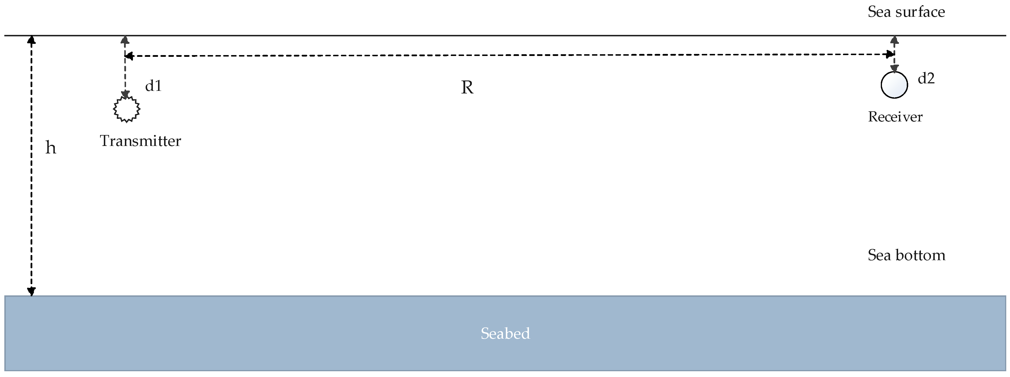
17]. The shallow water channel can be modeled using the Pekeris model [
18], as in
Figure 1, where the speed of sound propagation is constant in the whole layer.
In
Figure 1,
is the depth of the source node,
is the depth of the receiver,
is the depth of the area considered and
the transmission range. The distance along the direct path is calculated as [
18]:
The distance along different rays is given by:
where
is the path calculated when the first reflection occurs at the surface (
as number of surface reflections), while
represents the length of the path when the first reflection occurs at the sea bottom (
as bottom reflections). Equation (10) must be satisfied the condition:
, while the Equation (11) must be satisfied the condition:
.
If we consider a rough surface and this roughness is small compared to the wavelength, the reflection loss would be expressed through the scattering process. The reflectivity caused by a rough boundary [
14], is given by Equation (12):
where
is acoustic wave length
(),
is the new reflectivity coefficient reduced because of scattering at the rough interface,
is the incident angle,
expresses Rayleigh’s roughness parameter Equation (13), and
represent the rms roughness of the surface Equation (14), while
is the wind speed (m/s). In a smooth ocean surface, the reflectivity coefficient would be [
14]:
The surface lost [
19], is only used when the roughness coefficient is small, it is calculated as:
Rayleigh model is used for modeling the loss caused by the sea bottom reflection. This model considers the density and the speed of sound in the interface between water and sea bottom. Simplified Rayleigh model considers that the scattering phenomenon is not as important as in the sea surface which means the loss is frequency independent. To calculate the sea bottom loss we use [
15]:
where
and
being
and
density and sound speed in sea water, respectively; while
and
are the density and sound speed in the seabed, respectively. The angles of incidence
are not constant. They are determined based on the following formulas [
16],:
where
,
correspond to
and
, respectively as calculated by Equations (10) and (11). Delay is another important parameter in acoustic signal propagation. Let
be the propagation delay through the path of length
and
the propagation delay through the path of length
:
According to [
19], the delay is calculated as:
where
is the length of data packet (bits),
is the channel capacity (bps),
is the distance between the two nodes that are communicating, and
the propagation velocity of the acoustic wave in water (m/s), Δ
τ is the delay caused by multipath propagation. The first term represents the delay in data transmission, the second the delay in data propagation and the last one the delay caused by the multipath effect.
4. Applied Algorithm
To simulate the communication between the sensor nodes and to obtain the results from the underwater channel transmissions data we have studied and simulated the DEADS routing algorithm (Depth and Energy Aware Dominating Set Based Algorithm) [
20]. According to [
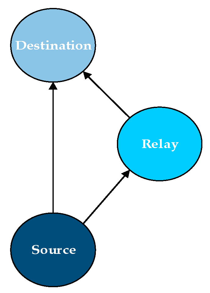
21], there two kinds of localizations: distributed and centralized. The nodes in our study have a randomly distributed localization in underwater environment and they have a predefined transmission range. It is also supposed that at the end of the broadcast phase, all the nodes will have information about the depth and the remaining energy of all their one hop away neighbors. The nodes send information on regular intervals about their remaining energy. As it is shown in
Figure 2, it is taken for granted the fact that source nodes are in the greater depth region and the relay and destination nodes are in the smaller depth regions, respectively.
To avoid flooding and its drawbacks our proposed change in algorithm as in [
20], uses a threshold value
which limits the outgoing links for every received packet. So, we calculate depth threshold as follows:
where
is the number of alive nodes inside the node’s transmission range,
is the total number of nodes in the network and
is the predetermined range of transmission for every node.
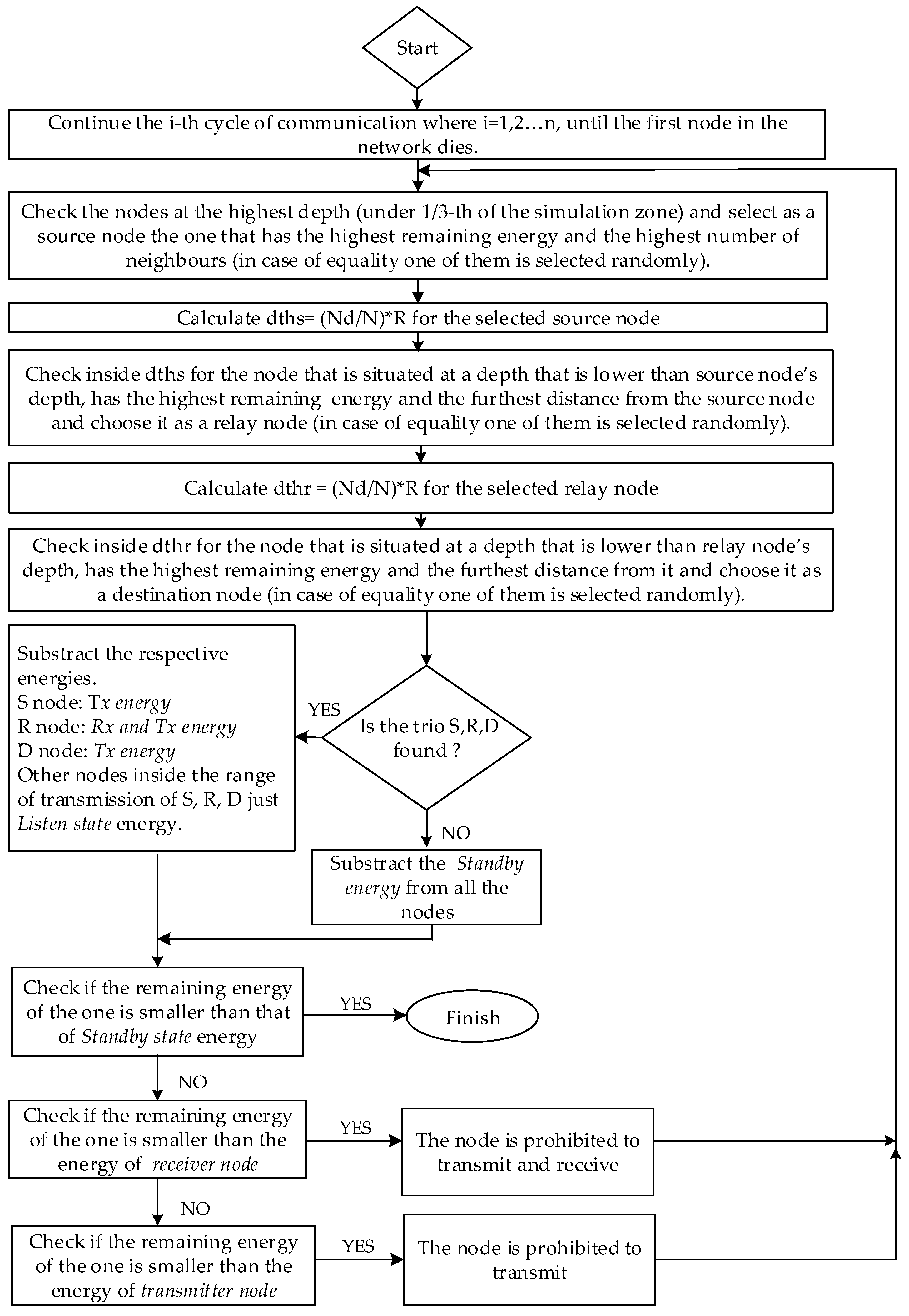
Thus, our approach minimizes the data propagation delay compared to the case where no depth threshold is used, because data will be transmitted in a shorter range. The performance of the algorithm, as shown in
Figure 3, is evaluated and the temperature, salinity and multipath effects are studied. The packet will be received by a node inside the
while all the other nodes outside of it will be considered in listening state (they listen to the information but do not receive it) so they will only spend energy in the listening state. The source nodes are selected based on the depth, by their highest remaining energy and the biggest number of neighbors. Then this node is selected in its depth threshold (
), it is checked for the other nodes that have lower depth than the source node, with the longest distance from it and the highest remaining energy, then the node is marked as a relay node. The same procedure applies also to the destination node selection. In every other case, like the cases when the end of network’s lifetime is approaching and nodes do not have the necessary energy to communicate, the standby energy is subtracted from every node’s remaining energy.
5. Simulations
According to [
22], some commercially available modems are considered: LinkQuest, Teledyne Benthos, TriTech International, Aquatec Group, EvoLogics and DSPComm.
Table 2 [
23] shows a number of commercial modems that are more suitable for dense networking with sensors in shallow areas, while
Table 3 shows the technical specifications of the EvoLogics modems that will be considered in the following. In this section, it will be measured the performance of the algorithm modified by us presented in
Figure 3. The network simulated has 50 nodes that are random distributed at a 200 × 200 m network. The initial power of each node is 4 J and the packet size to be transmitted is considered to be of 2000 bits. Any other parameters that are considered are shown in
Table 3. The basic metrics that will be taken in consideration are: (a) network lifetime (the number of communication cycles until the first node in the network dies), (b) the number of packets transmitted (a communication cycle is considered for the transmission for the entire packet, if it is transmitted successfully from the source node to the intermediate node and received from the destination node); (c) acoustic channel capacity in (kbps) (the average capacity of each acoustic channel between the transmitter and a receiver for a network whose environmental parameters will vary like: temperature or salinity); (d) delay (ms) calculated as the total delay needed to send the packet from the transmitter to receiver including the transmission delay (the time it takes for the modems to transmit the packet) as well also the propagation delay (the time it takes for the packet to propagate according to its direct path for the connection between the transmitter and the receiver).
Each graph and conclusion presented regarding the metrics mentioned, are as result of an averaging over 100 simulations.
5.1. Channel Performance as a Function of Different Salinity Values
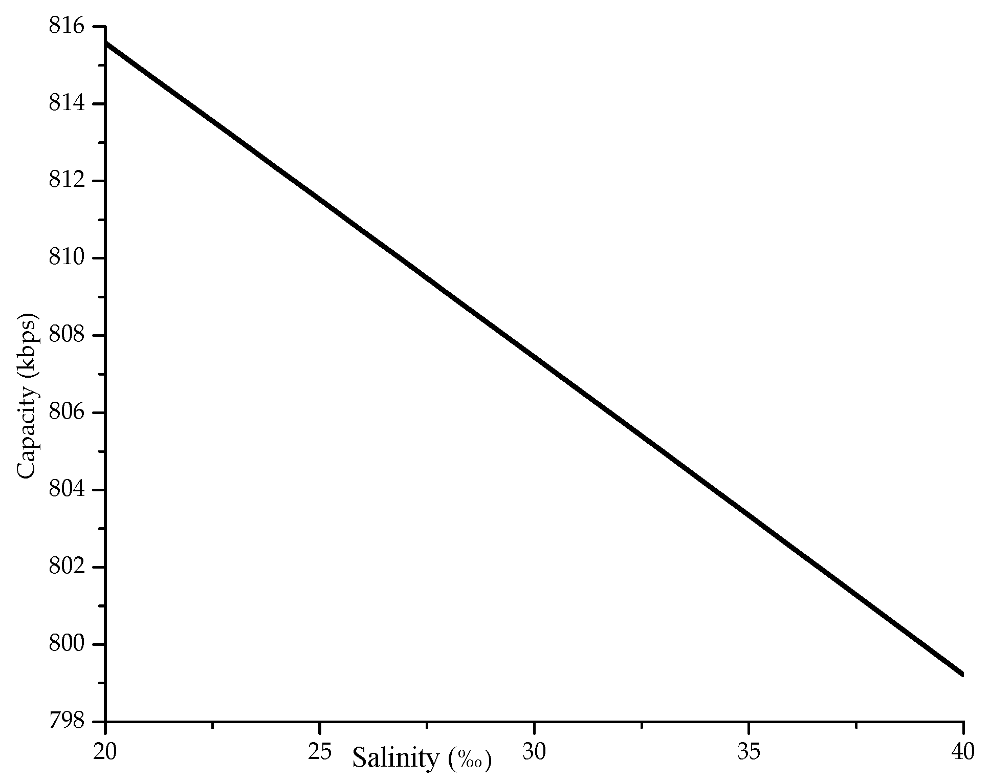
The first simulation is related to the effect of the salinity change on the acoustic channel parameters. So, salinity fluctuation is obtained between 20–40‰. Other parameters are fixed, like temperature at 29 °C, pH = 8, w = 5 m/s and frequency 78 kHz. The average value over all the capacities, obtained from Equation (8), of the acoustic channels of each node that communicated until the death of the first node for any network set up as a function of the salinity, ranging from 20 to 40‰, is shown in
Figure 4. By increasing salinity, the capacity of the acoustic channel decreases. This is because the increasing salinity affects the propagation of the acoustic communication path as it increases the absorption coefficient (increases the absorption term associated with magnesium sulfate). Increasing salinity would thus reduce the SNR ratio at the receiver and, according to Shannon-Hartley [
11], will be translated into a decrease in capacity.
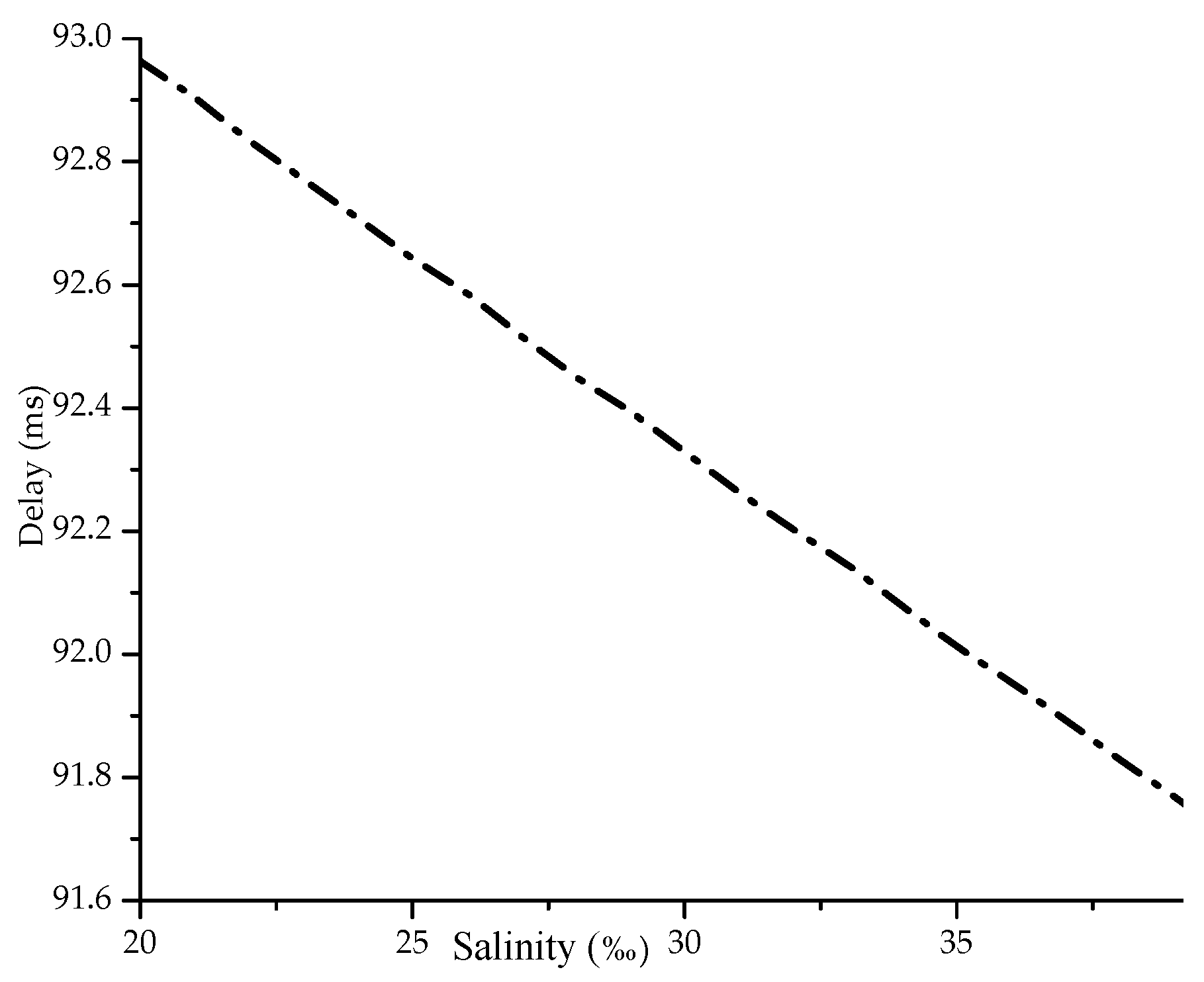
Figure 5 shows the performance of the total delay versus salinity, calculated according to the formula in [
25], brought here from Equation (22). With the increase of salinity coefficient, the total delay decreases. This is because the predominant component in the total delay is the propagation delay. As salinity increases the speed of sound propagation, the signal will require a shorter total time to propagate between the transmitter and the receiver.
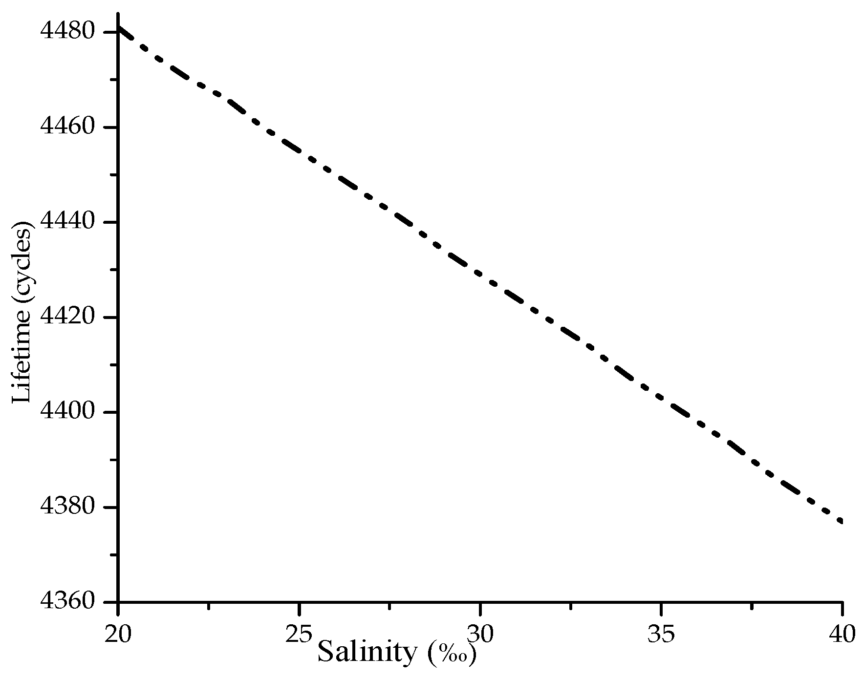
The results of simulations, following the algorithm introduced in
Figure 3, is presented in
Figure 6 and shows the lifetime performance of the algorithm depending on salinity, where as input are taken in consideration the energies presented in
Table 3.
The simulated results show that with the increase of salinity value, the capacity of the acoustic channel decreases, so the modem will required more time to transmit the data. The longer the transmission delay becomes, the longer the modems will operate to enable the packet transmission, and the more energy will be consumed as a consequence the network lifetime will decrease.
5.2. Channel Performance as a Function of Different Temperatures
Another environmental parameter whose variations are of great interest for studying on how it affects the capacity of the acoustic channels is the temperature. The temperature fluctuation is simulated between 17–29 °C. Other parameters were kept fixed are: salinity at 35‰, pH = 8, w = 5 m/s and frequency 78 kHz.
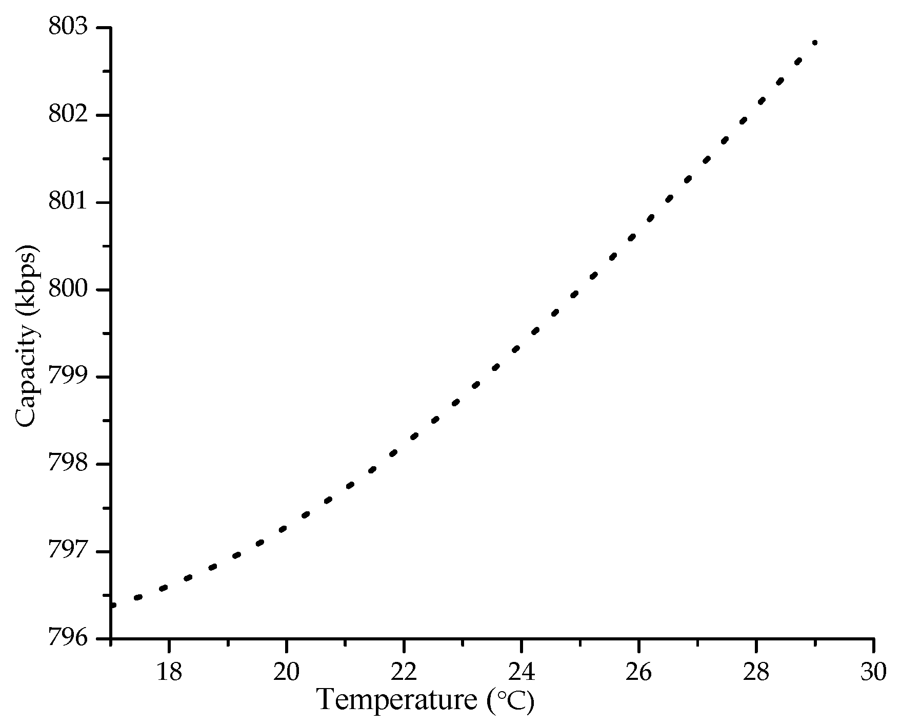
Figure 7 shows the performance of capacity, as obtained from Equation (8), versus temperature where the capacity is an average value for all communications that may have occurred in a network, when temperature varies between 17–29 °C, with step of 0.5 °C.
Capacity increases with the increase of temperature values, because the temperature affects the absorption coefficient by decreasing it. Thereby it helps in reducing the attenuation in the acoustic communication path and consequently by bringing an increase of SNR ratio in the receiver. At higher temperatures, this would increase the capacity of the acoustic communication channel by allowing more data to be transmitted per unit of time.
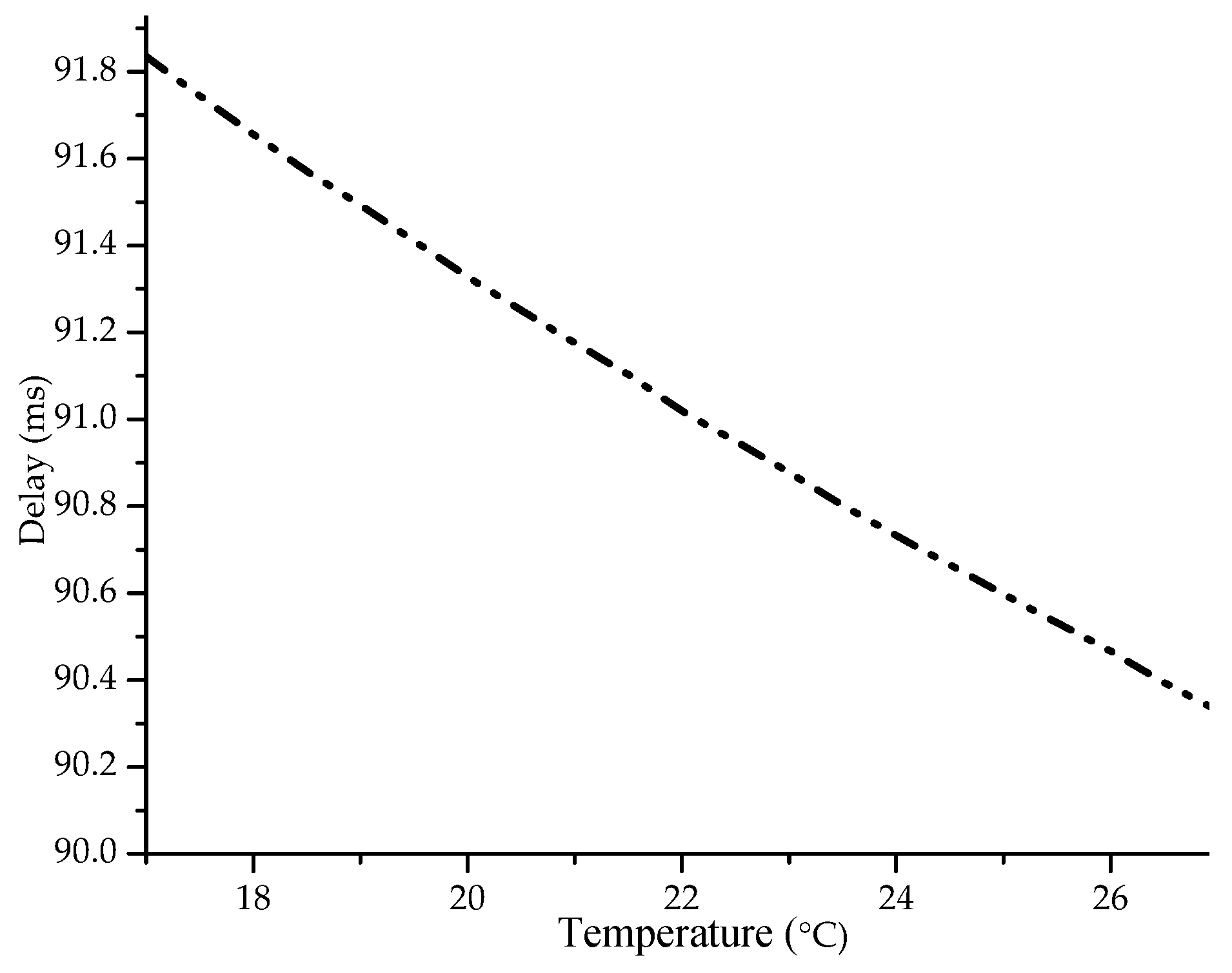
Figure 8 shows the performance of the total delay Equation (22) versus temperature changes.
The delay decreases with the increase of temperature values, because it decreases both the transmission delay (the modem takes less time to transmit the packet as the acoustic channel capacity is increased) and the propagation delay (as the temperature increases the acoustic signal spreads faster along the path). Reflections are not taken in consideration during these simulations as those will be estimated in the next section.
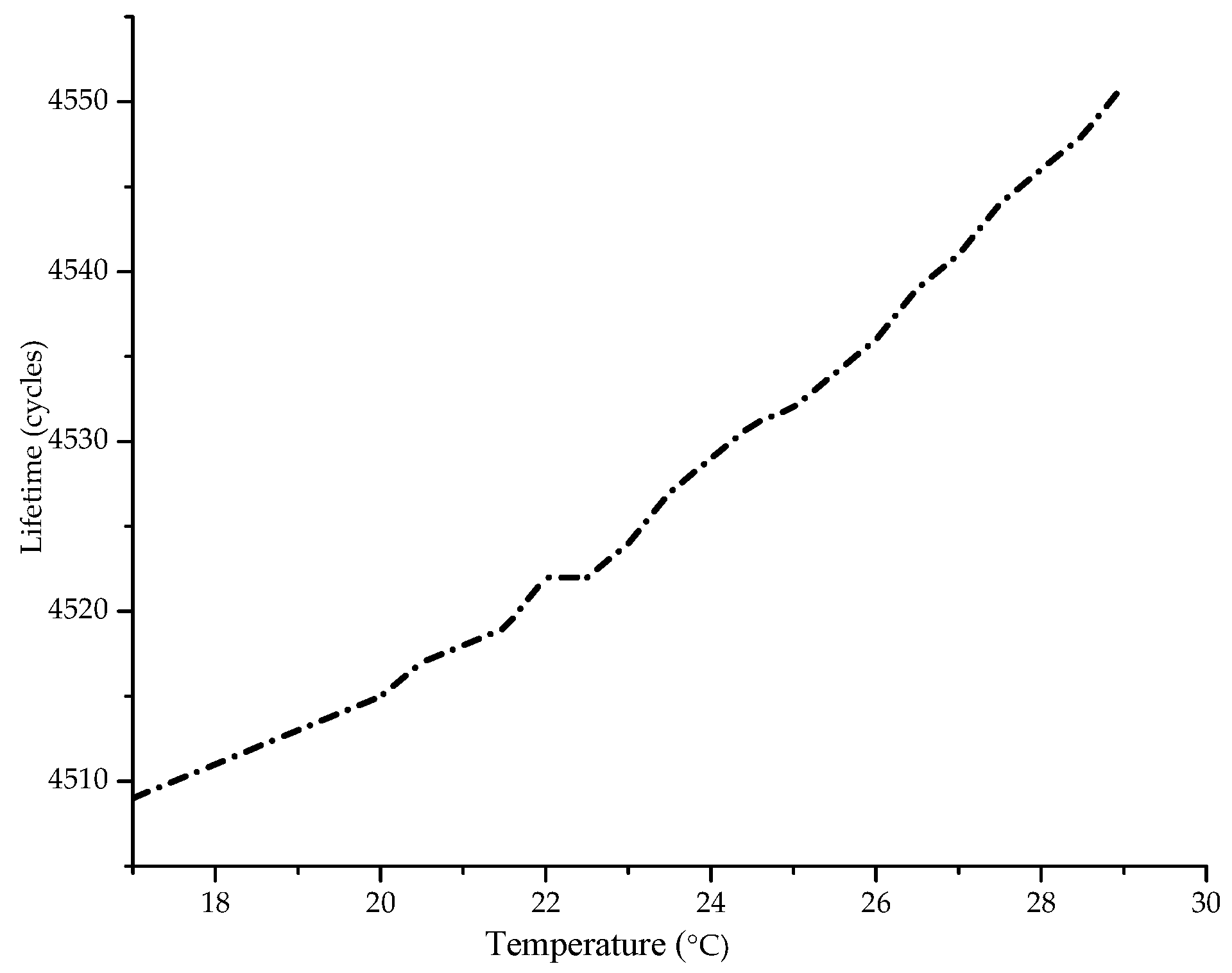
Figure 9 shows the performance of transmission lifetime as a function of increasing temperature. These metrics are increased with the increase of the temperature values, because it affects the overall capacity of the acoustic channel where more data can be transmitted per unit of time.
The time needed for the acoustic modem to transmit the packet in this way reduces energy consumption (longer lifetime) and leads to a larger number of packets transmitted.
5.3. Channel Performance in Presence of Surface and Bottom Reflections
The algorithm will enable the creation of a network of nodes where the dimensions and parameters used to set up the network are the same as those specified before. However, in these simulations, fixed parameters will be considered: S = 35‰, T = 29 °C, pH = 8, w = 1 m/s, f = 78 kHz, B = 30 kHz and c = 1500 m/s (speed of sound propagation). The nodes are distributed random in total depth [0, 200]. The nodes that are placed below 1/3 of the values of [0, 200] (the highest depth) are selected as sources nodes (
Figure 3). The relay node is selected by Equation (23) by being a node inside the depth’s range, (
Figure 3). The destination is selected by Equation (23) by being a node inside the depth’s range, (
Figure 3). The node that is almost in the surface of the sea, with the least depth. There will be an evaluation of some basic metrics like network lifetime, number of packets transmitted, acoustic channel capacity in (kbps) and total time delay in (ms). The first two metrics are evaluated in the same way as before, while the other two metrics i.e., capacitance and delay are averaged for each acoustic channel created for Tx/Rx communication, since in this case the number of reflections will vary according to [
12], caused to the fact that the propagation path into shallow areas can include from tens to hundreds of reflections.
The multipath phenomenon as well as the effects that this phenomenon brings to the acoustic channel capacity or network lifetime, will be simulated by considering a number of reflections where the first reflection occurs on the surface (each graph and conclusion presented with respect to the mentioned metrics is an averaged result 100 simulations performed). Evaluated metrics will also be compared in cases where oceanic bottom material changes, like volcanic rocks, limestone, sand, gravel whose geo-acoustic properties are shown in
Table 1.
The first simulation was performed regarding the effect of the number of reflections (multipath propagation) for an oceanic environment whose bottom material is made of basalt. Recall from
Table 1, that the velocity of sound propagation in this environment is 5250 m/s, much higher than 1500 m/s which is the velocity of sound propagation in water. According to the simulation presented in
Table 4, the channel capacity available for acoustic communication decreases as a result of the multipath effect (propagation according to many paths due to surface and bottom reflections). As a result, the SNR ratio in the receiver would decrease, a phenomenon which, according to Shannon-Hartley [
11], would be translated into capacity reduction. The effect of multipath has a stronger impact on capacity than environmental effects such as changes in temperature or salinity (it greatly reduces the capacity of acoustic communications) and that is why the multipath effect is one of the main problems of underwater environment.
Apart from the simulation carried out, the performance of the estimation metrics under the conditions of various materials at the bottom of oceans is of great interest. Recall that for these materials (basalt, limestone, gravel and sand), the sound propagation velocity ratios in those versus velocity of sound propagation in water (1500 m/s) are 3.5, 2, 1.2, 1.1 and material density ratios against water density (1000 kg/m3) are 2.7, 2.4, 2, 1.9.
Table 5 and
Table 6 present a comparison between the performance of acoustic communication capacity and lifetime for the four materials. The materials basalt and limestone referred to others (
Table 1) are less porous, and this results in smaller losses. Both capacity and lifetime decrease with increasing number of reflections. However, the acoustic communication capacity where the bottom area is basalt, would be higher than in an area of limestone bottom material. This is because in the latter losses as a result of bottom-up reflection would be higher, resulting in a decrease in the SNR in the receiver and a mandatory decrease in the amount of data transmitted per unit of time.
Considering lifetime, the simulations show (
Table 6) that by increasing the number of reflections the network lifetime decreases, as the acoustic communication capacity decreases. As a modem spends more energy during the transmission, this would increase the energy consumed for transmission and decrease the network lifetime.
Also, from
Table 7, results that as the number of reflections increases, the total delay will increase as in addition to the fact that the signal is transmitted to the receiver through longer paths. By increasing the number of reflections, the acoustic communication capacity decreases, so it will take even longer to send the packet. Two other bottom materials, sand and gravel, are taken into consideration in simulation presented in
Table 5,
Table 6 and
Table 7. Sand is the most porous material among the four materials mentioned. So, any reflected signal at a sand composite bottom environment would suffer the highest loss compared to the reflections in the other three environments, thus enabling lower acoustic capacity. The acoustic communication capacity performed in an area where the bottom environment is composed of gravel, would be higher than the capacity for a sand composite bottom material.
This is due to the loss that this material has on the reflected signal is much lower than the loss caused by the sand. Furthermore, lifetime decreases for basalt-limestone-gravel-sand crossings while the total delay to data acquisition would increase (decreased data transmission capacity). These results are also relevant for cases where acoustic modems will be designed for specific applications by the manufacturer.
6. Discussion of the Results
The simulation results presented in this paper show that achieving good performance in underwater communications in shallow areas is very difficult, since the presence of the multipath effect reduces the theoretical maximum communication capacity. So, the designer of a specific acoustic modem for a particular area must have knowledge of the ocean bottom material, in order to adapt the appropriate value of the data transmission capacity of the acoustic link.
In the first part of the paperpaper it was shown the impact of increasing salinity and temperature within a range of values similar to the real ranges of values for these parameters in many underwater environments and coastal areas. We have simulated a network with dimensions of shallow areas and there are taking into account the parameters of the S2C R 48/78 acoustic modem. Capacity and total delay lifetime have been estimated as a function of the temperature and salinity values. The result is that a network in shallow areas where surface temperature is higher results in higher communication capacity utilization compared to a network in shallow area where the surface temperature is lower. Obviously, under higher surface temperature conditions, the network lifetime is longer because more data are transmitted per units of time, the acoustic modem would consume less energy in transmitting packets where the transmission time of a unit individual packages are lower. On the other hand, the nodes of a network in a shallow area where salinity has higher values would utilize a lower acoustic channel capacity for communication between them compared to the capacity that would utilize the nodes in an area with lower salinity. This is because the increase in salinity increases the losses due to absorption, causing the SNR in the receiver to decrease, which would be translated into a decrease of the channel capacity. The total data propagation time from transmitter to receiver, as a combined parameter between transmission and propagation delay, decreases with increasing of both salinity and temperature values. This happens because the acoustic waves propagate more rapidly underwater in both cases.
The effect of multipath propagation has also been evaluated in this paper, where the simulations are applied at depths of up to 200 m. The receiver node gets data from both the direct path in less time and the reflection paths formed by the surface and bottom at longer time. Losses in surface reflections increase if surface roughness or surface wind speed increases. On the other hand, losses due to bottom reflections depend on bottom material of the ocean bed. So, another conclusion of this paper, thus related to the effects of the bottom materials, is that the acoustic communication capacity available is higher if the bottom material is less porous compared to the case of a more porous material. For example, such as in sand where the capacity utilized for acoustic communication and the lifetime of a network in an area with such bottom material is lower. This is because for a less porous material the reflection losses at the water-bottom material are higher.


