Toward Scalable Video Analytics Using Compressed-Domain Features at the Edge

Abstract

Intelligent video analytics systems have come to play an essential role in many fields, including public safety, transportation safety, and many other industrial areas, such as automated tools for data extraction, and analyzing huge datasets, such as multiple live video streams transmitted from a large number of cameras. A key characteristic of such systems is that it is critical to perform real-time analytics so as to provide timely actionable alerts on various tasks, activities, and conditions. Due to the computation-intensive and bandwidth-intensive nature of these operations, however, video analytics servers may not fulfill the requirements when serving a large number of cameras simultaneously. To handle these challenges, we present an edge computing-based system that minimizes the transfer of video data from the surveillance camera feeds on a cloud video analytics server. Based on a novel approach of utilizing the information from the encoded bitstream, the edge can achieve low processing complexity of object tracking in surveillance videos and filter non-motion frames from the list of data that will be forwarded to the cloud server. To demonstrate the effectiveness of our approach, we implemented a video surveillance prototype consisting of edge devices with low computational capacity and a GPU-enabled server. The evaluation results show that our method can efficiently catch the characteristics of the frame and is compatible with the edge-to-cloud platform in terms of accuracy and delay sensitivity. The average processing time of this method is approximately 39 ms/frame with high definition resolution video, which outperforms most of the state-of-the-art methods. In addition to the scenario implementation of the proposed system, the method helps the cloud server reduce 49% of the load of the GPU, 49% that of the CPU, and 55% of the network traffic while maintaining the accuracy of video analytics event detection.

1. Introduction

Today, the world is witnessing an exponential increase in camera deployment [1]. According to IHSMarkit’s annual report [2], as of 2018, China has one camera for each 4.1 people in the country and the United States has a people-to-camera ratio of 4.6:1. The massive deployments of cameras are brought on mainly by the growth of the video surveillance industry due to increasing concerns about public safety and security. With such a prevalent trend, intelligent video analytics systems have been playing an essential role, performing important tasks in various fields including surveillance, transportation, manufacturing, etc.

Figure 1 illustrates a traditional cloud-based video stream analytics system. A large number of cameras transfer video data to a central cloud where video analytics is performed. However, this traditional approach makes it difficult to perform real-time analytics on live video streams from many cameras because the video analytics involves several computation-intensive tasks such as object detection, object tracking, object recognition, and so on. Besides, streaming video from multiple cameras to the cloud consumes much network bandwidth over limited-bandwidth networks, which leads to high latency, causing significant challenges for real-time video analytics.

To address these challenges, we aim to develop a solution by harnessing edge computing. Video analytics at the edge has multiple benefits such as decreasing the response time, saving network bandwidth, and minimizing the peak workload to the cloud. However, edge devices are typically much less powerful than the cloud, with limited computing resources such as a few GPUs (graphics processing units) and CPUs (central processing units), as well as smaller RAM (random access memory) capacities [3]. In the field of public safety, the ability to simultaneously process multiple feeds and provide real-time video analytics is critical. Therefore, this study seeks to answer how edge devices and the cloud can cooperate in an efficient manner to achieve real-time and scalable video analytics.

One of the features frequently observed in surveillance camera images is that captured images remain unchanged for a long time and that video content is often quite redundant. Therefore, it is undesirable to conduct analytics on redundant video frames from cameras, leading to a waste of computing resources and power consumption in the cloud. Motivated by this, we propose a pre-processing module that acts as a video filter function at the edge device to eliminate the redundant static images before feeding videos to the cloud for further analysis. The proposed method runs on an edge device and recognizes the motions (i.e., moving objects) in the consecutive video frames. Based on the motion recognition result, our module decides whether to pass the video frame to the cloud or filter it out. As a result, the proposed motion-based filtering module can reduce not only the computational load of the cloud nodes, but also network traffic to the cloud.

Motion recognition schemes can be classified into two categories: (i) video pixel-domain-based and (ii) video compressed-domain-based approaches. In pixel-domain-based approaches [4,5,6,7], the video is completely decoded before using background modeling or the vision-based deep learning framework to detect moving objects at the pixel level. The performance of video pixel-domain processing in large systems may be challenged by the load of decoding multiple streams and the image pixel-based calculation. Thus, the pixel-based approach requires higher computational complexity and can make it difficult to fulfill the real-time requirement of edge devices. Compressed-domain approaches [8,9,10,11] rely on video coding artifacts of compressed bitstreams such as the motion vector (MV), macroblock partitions, and quantization coefficients for recognizing motion. Compared to pixel-domain-based algorithms, compressed-domain methods generally require less computational resources because analyzing input information is already possible in the bitstream.

In this study, we propose a compressed-domain-based moving object detection that applies a data clustering and an intersection over union (IoU) rate-based object tracking technique of computer vision. Using only MVs, which are provided by video encoders in a compressed bitstream, our approach is able to efficiently detect moving objects. Furthermore, an experimental evaluation of our method is provided to compare it with the state-of-the-art compressed-domain tracking methods in terms of processing time and demonstrate its functionalities to evaluate the efficiency of the proposed edge device with a cloud video analytics server in a real-world scenario. In summary, this paper makes the following contributions.

• Introduction of a compressed-domain moving object detection method that can be applied in numerous surveillance applications.
• Design of an edge-to-cloud computing system for surveillance video analytics that applies the proposed method at edge devices to minimize the transfer of video data from surveillance camera feeds to the cloud.
• Implementation and evaluation of the proposed method with an edge-cloud system. The implementation is lightweight and easy to deploy at any edge devices.

The remainder of this paper is organized as follows. Section 2 describes the background knowledge of video coding MV and the related state-of-the-art algorithms for moving object detection in both the compressed-domain and pixel-domain. Section 3 describes the proposed system based on the video coding MV analysis method for moving object detection. Section 4 presents the implementation and evaluated results. We summarize the contribution of this study and present our future directions in Section 5.

2. Background

There are many different approaches to video moving object detection, both utilizing compressed and uncompressed data. In this section, we briefly introduce the state-of-the-art approaches for moving object detection in both the compressed-domain and pixel-domain.

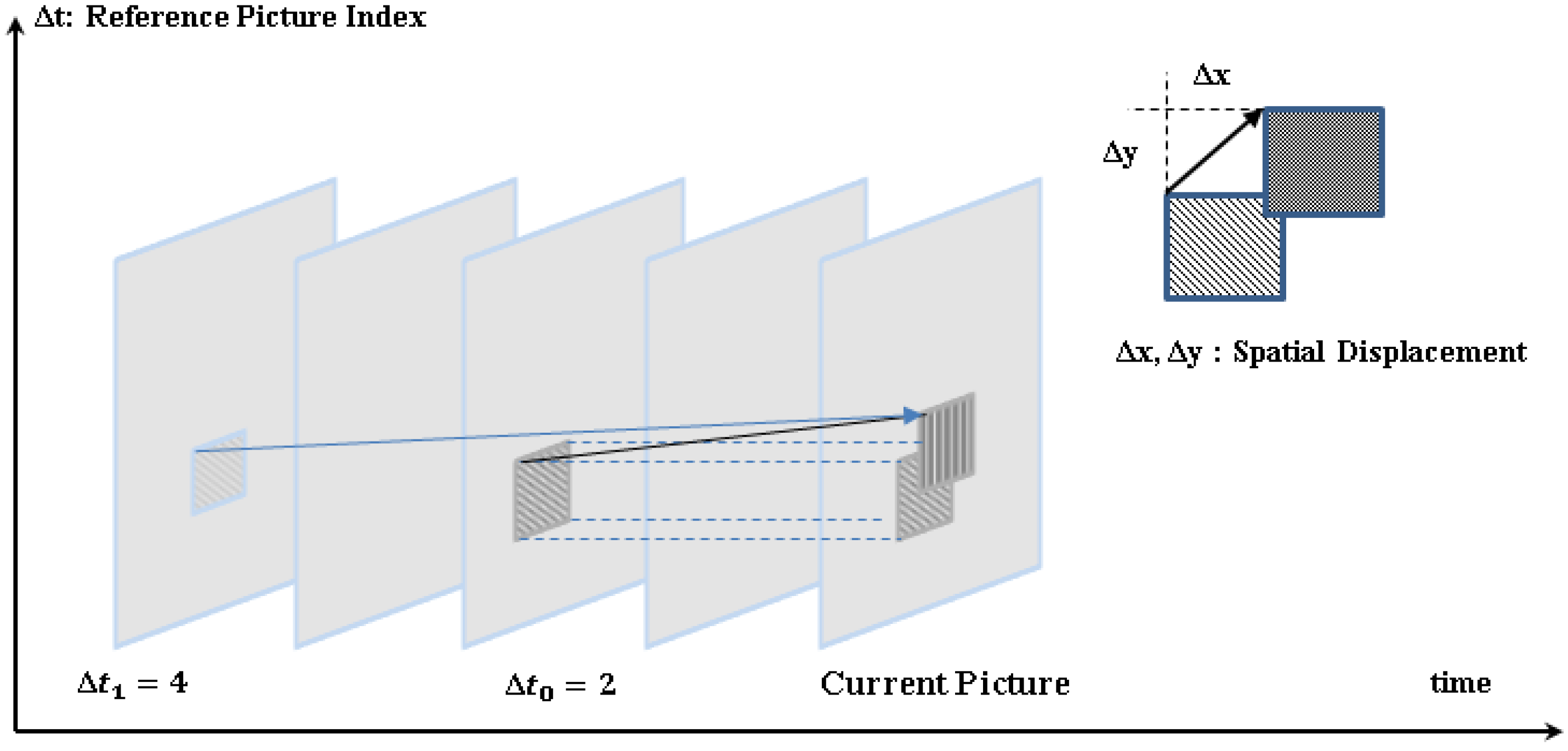
2.1. Compressed-Domain-Based Moving Object Detection

The traditional video coding standards, such as MPEG-1, MPEG-2, H.264, and H.265, are based on the motion estimation process, which involves identifying a correspondence among consecutive images. In video coding standards, the MVs of a current block are correlated with the MVs of neighboring blocks in the current image or in the earlier coded pictures [12,13]. While intra-picture prediction exploits correlations between spatially neighboring samples, inter-picture prediction makes use of temporal correlation between images to derive a motion-compensated prediction (MCP) for a block of image samples [14].

For intra-prediction, we assume that neighboring blocks possibly correspond to the same moving object with similar motion and the motion of the object is not likely to abruptly change over time. Consequently, using MV in neighboring blocks as the predictor reduces the size of the signaled motion vector difference. For this block-based MCP, a video image is divided into rectangular blocks. Figure 2 shows the general concept of MCP based on a translational motion model. Using a translational motion model, the position of the block in a previously decoded picture is indicated by a motion vector $(\Delta x,\Delta y)$, where $\Delta x$ specifies the horizontal and $\Delta y$ the vertical displacement relative to the position of the current block. Note that the motion vectors $\Delta x$, $\Delta y$ could be of fractional sample accuracy to more accurately capture the movement of the underlying object. These MVs are coded by entropy coding and placed into a compressed bitstream for delivery to the video decoder, which uses MVs, along with one or more previously decoded pictures, to reconstruct the current image. Therefore, MV information indeed follows the real motion of objects and can be used for tracking.

On the other hand, H.264/AVC (Advanced Video Coding) in view of higher resolution and low bandwidth utilization and storage requirement becomes the popular video compression standard for surveillance video. In H.264/AVC, each video sequence is divided into groups of pictures (GOP), comprising at least one intra-code I frame, uni-directionally predicted P frames, and bi-directionally predicted B frames. Typically, the first frame in a GOP is the intra-coded I frame followed by the P and B frames. The I frame uses raw data from the camera, while other frames in a GOP utilize the predictive coding involving motion vectors’ displacement. Each frame is partitioned into rectangular areas called macroblocks that are further partitioned into variable size blocks. The motion compensation of displacement is performed at the macroblock and block levels for all intra-coded frames. In the process of motion compression, MVs are obtained for each motion block between the current and reference frames. By minimizing the prediction residual, the MVs represent the temporal displacement between the two block.

In recent studies, compressed-domain-based video analytics methods [15,16] that rely on video coding artifacts of compressed bitstreams, such as MVs, macroblock partition, and quantization coefficients, have been proposed. In [15], the authors applied a probabilistic technique of computer vision for image separation, known as graph cut [17], modeling with MVs rather than pixels and adapted to the additional temporal dimension of video signals. MVs and a spatio-temporal Markov random field (ST-MRF) model that naturally integrates the spatial and temporal aspects of the object’s motion for tracking were used. In general, these approaches do not rely on pixels and studies by only using the codec’s MVs and block coding modes’ extracted bitstream through inexpensive partial decoding. In this manner, computing and storage requirements have been significantly reduced compared to the “pixel-domain”.

The primary limitation of this approach is that it may lead to a noisy MV field that does not necessarily correspond with the actual object movement of the object in the scene, as shown in Figure 3. The noisy MVs fail to provide useful information such as attributed to illumination changes and background movement. The amount of noise MVs is relatively reduced compared to the correctly estimated MVs because noisy vectors are continuous and similar for MVs from real moving objects. Another challenge of this approach is the lack of information about the object’s appearance such as color, edges, and texture, because these features would require complete decoding of the compressed bitstream. In this study, our aim is to work in the “compressed-domain” and use only the MVs from the compressed bitstream to detect and track moving objects in video frames.

2.2. Pixel-Domain-Based Moving Object Detection

Due to more reliable features that can be extracted from the pixel data, the majority of moving object detection methods require full decoding of the video stream. In the pixel-domain, a video analytics server analyzes the red-green-blue image to determine the appearance of objects and spatial events. Ubiquitous real-time video analytics remains an open and exciting research problem, and it is fueled by the recent advantages of hardware and deep learning [18,19,20,21,22,23]. There are two primary methods that are considered for moving object detection in the pixel-domain.

2.2.1. Hybrid Model of Background Subtraction and Object Classification-Based Moving Object Detection

The background subtraction method [24,25] subtracts the current frame and background image to eliminate an image’s background and then detects moving targets based on gray value differences. This method is the most commonly used object detection technique. There are a number of methods that have been used to build the background model, e.g., [26] proposed a novel real-time motion detection algorithm that integrates the temporal differencing method, double background filtering method, optical flow method, and morphological processing methods to obtain excellent performance. Moreover, the authors of [25] discussed modeling each pixel as a grouping of Gaussians using an on-line approximation to renew the model. The Gaussian distributions of the adaptive mixture model were then assessed to determine which model can be presumed to be obtained from a background process. This method’s advantage is its simple implementation, low computational resource requirements, robustness in the presence of environmental noise, and dynamic background. However, it has limitations with shadows, background changes, as well as object localization and classification. Furthermore, object detection based on the background model cannot detect the individual objects in a group or a block object. In general, the aim of background subtraction is to separate foreground images from background ones in the form of blobs, followed by an object classification process. The detected blobs then help classify each blob into subclasses, as shown in Figure 4, which shows the complete process of this approach to perform smoke detection. Fortunately, deep learning, a relatively new technique in machine learning, enables very accurate classification of images using convolutional neural networks (CNNs) [27,28,29]. The capacity of CNNs can be controlled by varying their depth and breadth; moreover, they make strong and mostly correct assumptions about the nature of images (i.e., stationarity of statistics and locality of pixel dependencies). For example, by combining CNN and transfer learning, the authors of [30] achieved an average accuracy of 70.1% using the CIFAR-10 [31] dataset.

2.2.2. Deep Learning-Based Moving Object Detection

Hybrid background subtraction and deep learning classification enhance the system’s accuracy; however, there are issues with the detection of individual objects in a group or blocked objects and the background changes by the lighting condition and the environmental noise. Hence, the usage of deep learning is considered for robust object detection tasks. We identified three primary object detection methods using deep learning:

• R-CNN, Fast R-CNN, Faster R-CNN
• You only look once (YOLO)
• Single shot detectors (SSDs)

R-CNN [32] uses selective search [33] to extract several regions, called region proposals, from the image; it then attempts to classify a large number of regions. Each region proposal is placed into CNNs to extract features, which are fed to a support vector machine to classify the presence of objects within the candidate region proposal. The limitation of this method is that it requires a large amount of time to train and deploy networks because it has to classify multiple region proposals per image. Fast R-CNN [34] solves the limitations of R-CNN by putting the entire image into the CNNs to generate a convolutional feature map and identify the region proposals based on the map, thus reducing the number of classified region proposals. Both R-CNN and Fast R-CNN use selective search to identify the region proposals. Selective search is a slow and tedious process that affects the network’s performance. Faster R-CNN [35] was proposed to allow the network to learn the region proposals; it uses a separate network to predict the region proposals rather than using a selection search algorithm on the feature maps’ output using the CNN layer. YOLO [36] is an object detection system targeted for real-time processing. Unlike R-CNN, Fast R-CNN, and Faster R-CNN, which use regions to localize the object within the image, YOLO uses a single neural network to predict the bounding boxes and the class probabilities for these boxes during the training and test periods. Hence, YOLO only examines the input picture once to predict the presence and location of objects. YOLO divides the input image into an S × S grid, and multiple bounding boxes can exist within each grid. For each bounding box, the network outputs a class probability and offset value for the bounding box. The bounding boxes with class probabilities above a certain threshold value are then selected and used to locate the object within the image. Note that YOLO has 24 convolutional layers, followed by two fully connected layers. The initial convolutional layers of the network extract features from the image, while the fully connected layers predict the output probabilities and coordinates. According to the performance comparison in [37], YOLO is faster (45 frames per second (FPS)) than the other object detection algorithms. Faster R-CNN is more accurate than YOLO (a mean average precision (mAP) of 73.2, as compared to 63.4); however, YOLO is considerably faster than Faster R-CNN (FPS of 45, as compared to seven). Therefore, SSDs [38] were released as a balance between these two methods. Compared to YOLO, an SSD runs an input image through a convolutional network only once and computes a feature map. Then, a small 3 × 3 sized convolutional kernel is run on this feature map to predict the bounding boxes and categorization probability. Moreover, SSD uses anchor boxes at various aspect ratios comparable to Faster RCNN and learns the offset to a certain extent compared to learning the box. The SSD is able to detect objects of multiple scales because every convolutional layer functions at a diverse scale. Compared to the YOLO method [37], SSDs attain similar accuracy, but run slower. In this study, YOLO was applied to robust human detection at cloud servers for our implementation.

3. Methodology

In this section, the proposed edge-to-cloud system for surveillance video analytics applications is presented in detail. Then, the method for moving object detection in the compressed-domain is analyzed. In addition, the performance evaluation model for video analytics platform is introduced.

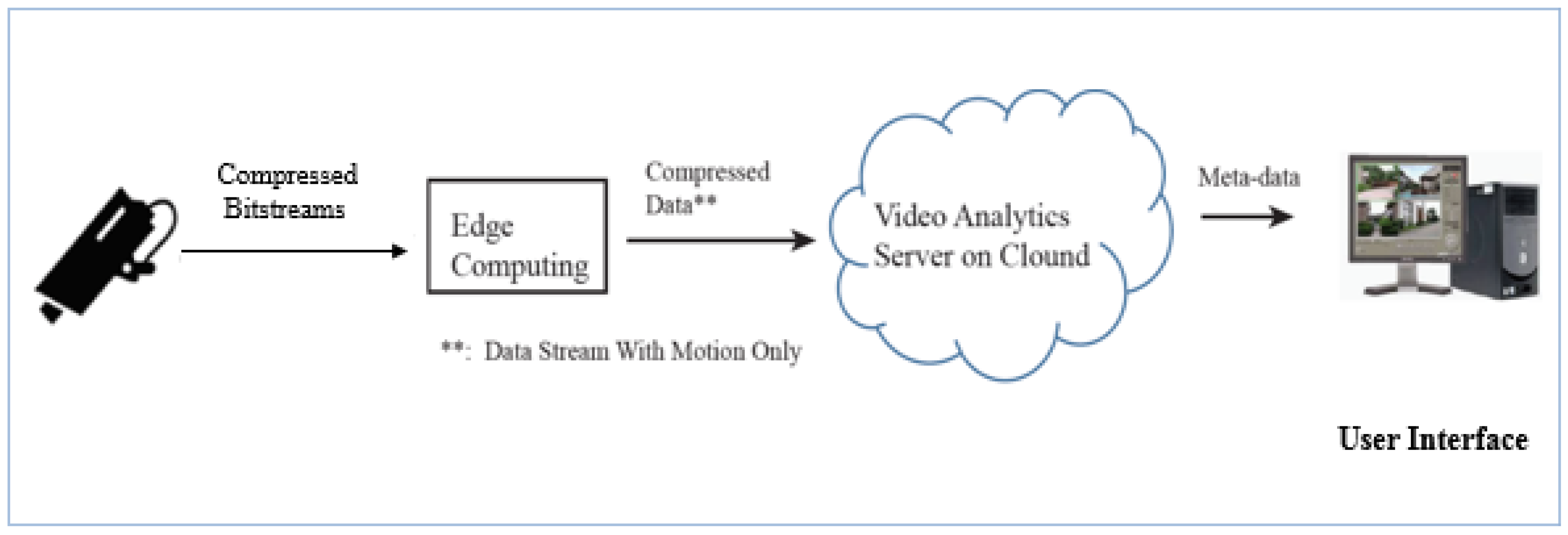
3.1. The Edge-to-Cloud System Model for Surveillance Camera-Based Applications

There is a trend to forward computation from the network core to the edge where most of the data are generated. Edge computing has exhibited its potential in reducing the reaction time, minimizing bandwidth usage, and improving energy efficiency. Edge computing performs data processing at the “edge” of the network, close to the data source. For network cameras, audio, and other sensors, there is a need to balance both cloud computing and edge computing domains to deliver refined, reliable, and usable data. For edge computing of delay-sensitive video tasks, a camera source node can offload its video task to nearby edge nodes via local wireless/optical networks, and edge nodes are within the local communication range of the camera. The camera captures the video sequences and divides each of them into multiple video chunks, compresses these video chunks, and then, delivers them to edge nodes. Next, edge nodes implement video processing functions on the received video chunks and upload the results to a cloud server for video analysis (such as object/event detection). A delay-sensitive video assignment is supposed to be processed within a limit and will fail if the deadline is passed. In this study, as shown in Figure 5, we consider an edge computing network, which comprises three primary components, namely the camera source node, edge node, and cloud server.

• Camera source node: The camera node periodically generates video tasks, divides each video task into a number of video chunks, compresses the video chunks at certain compression ratios, and then, assigns the compressed video chunks among all edge nodes as per scheduling policies.
• Edge node: The edge has computational ability and storage capacity and helps preprocess video chunks. Moreover, edge nodes can form cooperative groups based on the specific group formation policy and receive compressed video chunks as per the video load assignment policy.
• Cloud server: The cloud server collects the preprocessing results from edge nodes, which has abundant computational abilities, and performs additional video analysis.

During a sparse edge node deployment, an edge node will only connect to one of the available cameras at a certain location; however, in a dense deployment, an edge node may have multiple choices for selecting multiple cameras. In this study, we focus on reducing processing load on the cloud server by minimizing the video chunks that are fed from the camera sources. Therefore, an edge device runs preprocessing tasks to filter uninteresting video chunks. The term “uninteresting video chunks” is defined via scenario specification: for surveillance scenarios, it is static scenes without any objects and gradual changes.

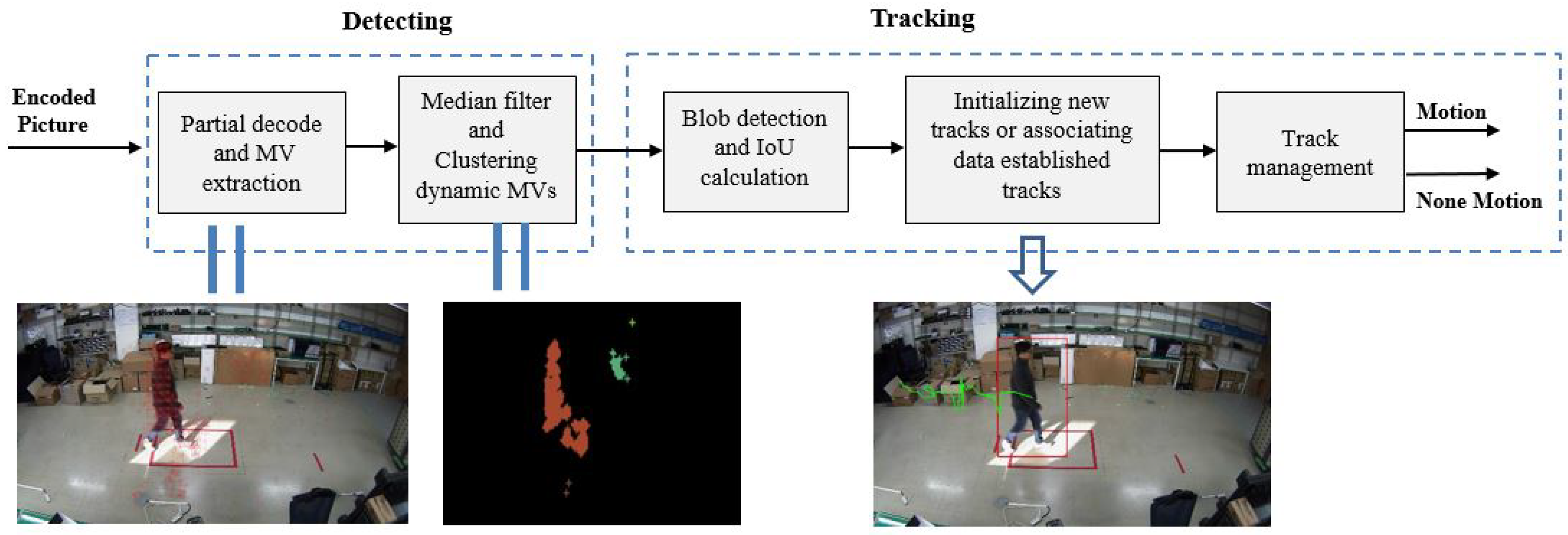
3.2. Light-Weight Runtime Moving Object Detection in the Video Compressed-Domain

As mentioned in Section 2.1, the aim of this method is to analyze only MVs at the edge device, recognize the real moving objects, and exclude the noisy motions that are generated by environmental factors such as illumination changes and background movement, in the current video scene. For this purpose, we present a method that has the workflow shown in Figure 6 to analyze the video coding MVs. In order to extract MVs from the compressed bitstream, the input video stream is partially decoded, and the collected MVs include both real object MVs and noise MVs. Examples of extracted MVs are represented in Figure 7 in consecutive frames of two different video test sequences. To analyze these MVs, the following functionalities are involved.

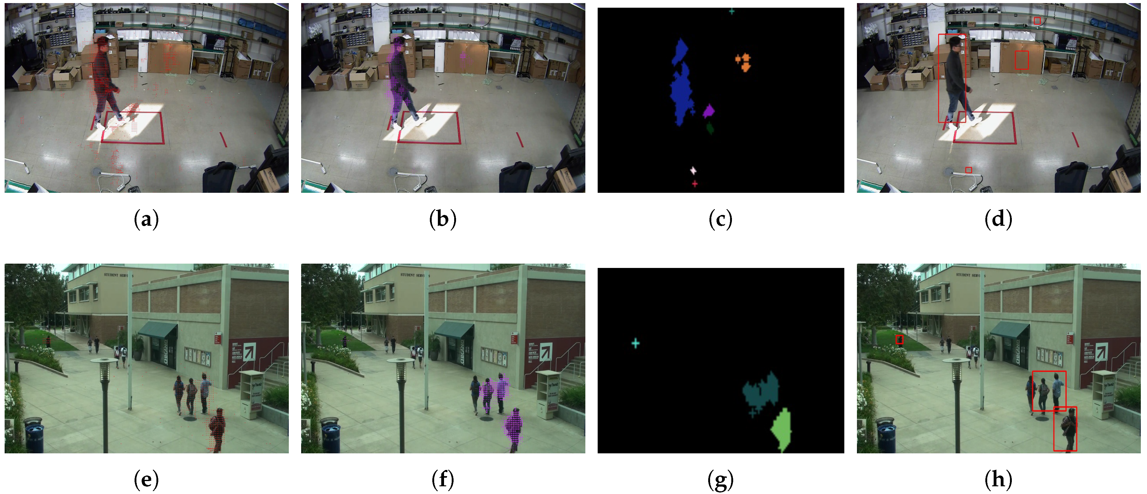
3.2.1. Median Filter and Moving Object Detection

Compressed-domain MVs may not represent the actual true motion due to the properties of motion estimation, biased towards efficient coding, as shown in Figure 8a,e. Therefore, it is desirable to eliminate motion vectors that can be categorized as unsuitable for moving object detection. We assume that MVs whose magnitudes are very high or very low, compared to the other MVs related to the moving object, have to be replaced with the median value of neighboring MVs. Therefore, the application of the vector median filter aims to reduce isolated vector noises and smoothen the difference of MV between adjacent blocks. Note that the sliding window approach is used for median filtering. Because H.264/AVC allows for variable-sized block partitioning, we construct a uniformly sampled MV field by mapping all MVs to 4 × 4 blocks. Theoretically, the motion vector average (normalized vector) among all elements $N_{mv}$ in the N × N (N = 4 in this study) window function is calculated by Equation (1):

$$N_{mv}=\frac{{\sum }_{i=1,j=1}^{N\times N}M{V}_{ij}}{N\times N}$$

(1)

where $M{V}_{ij}$ is the MV elements in the N × N window. Finally, the smoothened motion filter is presented, which is experimentally determined as shown in Figure 8b,f using the input MV, including isolated motion vector noise, smoothened in the areas that mostly correspond to the object boundaries. In order to detect the moving objects, a cluster detector is involved to determine the number of moving objects and their approximate positions in the scene. Then, a density-based cluster technique is applied to completely segment moving objects. The first step involves MVs whose magnitudes can be used to easily differentiate moving objects from the stationary background. However, it is difficult to directly and completely segment moving objects because not all MVs on the objects have the same motion state. While every part of a rigid body maintains nearly the same motion state, different parts of a non-rigid body can move in various ways (see Figure 9). In order to cluster detected MVs into dynamic clusters, a range search algorithm based on the euclidean distance of the MV point is used, under the presumption that dense points represent the same object. This requires a parameter $\epsilon$ where $\epsilon$ is the spatial distance threshold between density reachable MV. The goal is to partition n MV points $\chi \subset {\mathbb{R}}^d$ into k clusters using the k-means filter. Each of the n data points will be assigned to a cluster with the nearest mean. The mean of each cluster is called its “center”. For the k-means problem, we wish to choose k centers $\mathbb{C}$ so as to minimize the potential Equation (2):

$$\varphi =\sum _{x\in \chi }^{}\underset{c\in \mathbb{C}}{min}{∥x-c∥}^2$$

(2)

From these centers, we can define a clustering by grouping data points according to which center each point is assigned. With MV points, the following steps are performed frame by frame:

• For each $p_i\in \chi$, find all the neighboring points within spatial distance $\epsilon$.
• Cluster all the MV points that are density reachable or density connecting [39] and label them.
• Terminate the process after all the MV points are checked. The output is a set of clusters of dynamic points.

The distance threshold $\epsilon$ decides the range of density reachability [39].

After this process, the label list includes the moving objects and certain big MVs’ noises, as shown in Figure 8c,d. To eliminate these noises, we based the observation on the fact that noise motions because of lighting condition changes usually randomly occur without following a certain flow. Therefore, the tracking motion’s trajectories’ length is then used to classify the detected motion into the real motion or noise group. If the object tracking trajectory length is larger than a certain threshold, it indicates that the objects move as a flow and the time is sufficiently long to consider it as a real motion. Moreover, the I Frame does not apply the motion estimation process; therefore, the MV analysis process will be skipped for I frames. In order to overcome the discontinuous object detection process, the object tracking algorithm will also be applied to derive the moving object’s bounding box in the I frame based on the last states in the P frames. As mentioned in Section 2.1, the IoU-based object tracking is applied to track motion because it is a light-weight and widely tracking algorithm that calculates the overlap area between two bounding objects. Note that this tracking was implemented and evaluated in some previous studies [40,41].

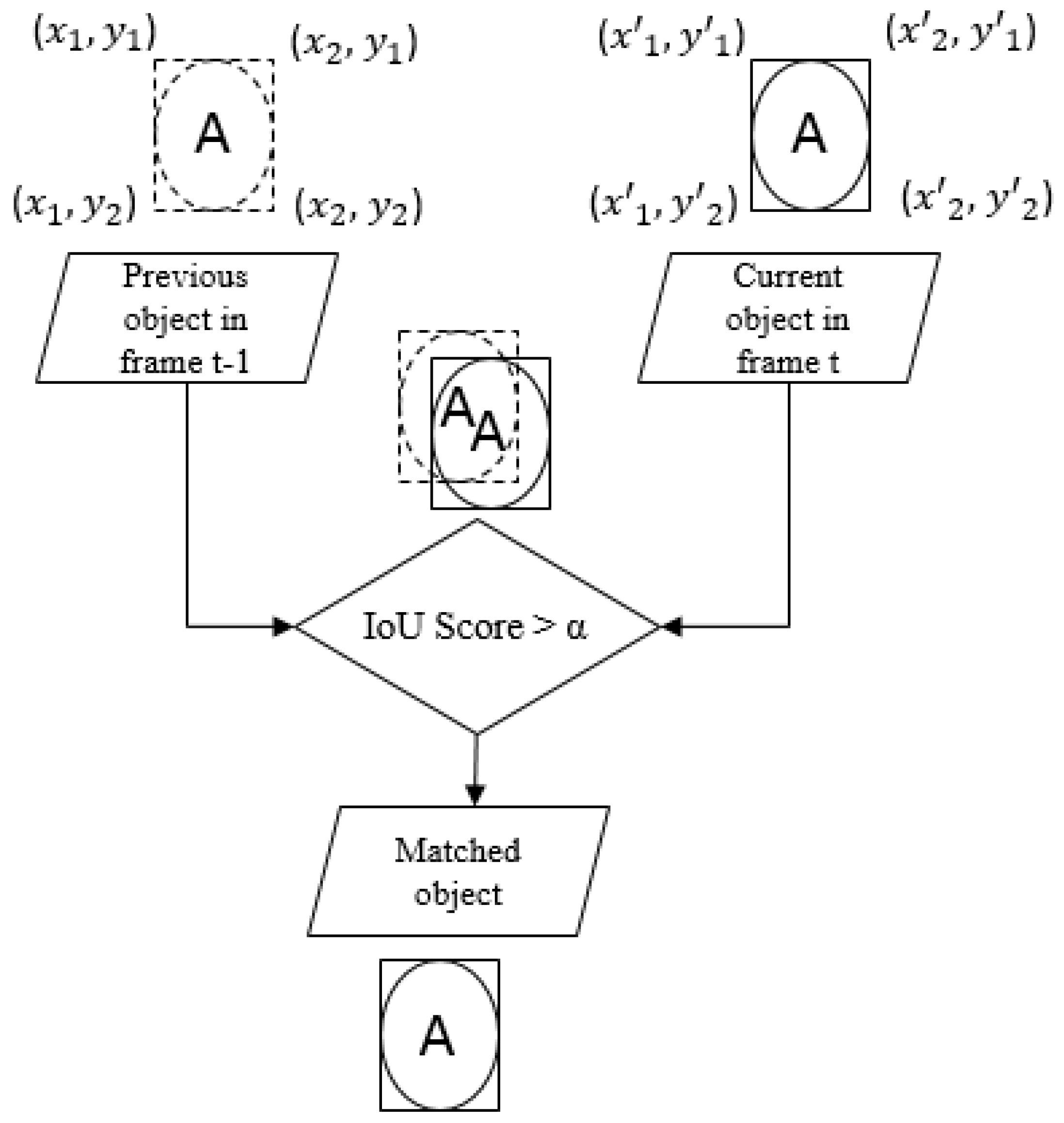
3.2.2. IoU-Based Moving Objects Tracking

To apply the IoU-based object tracking, the detected clusters are normalized with a rectangle bounding box according to the cluster’s size, as shown in Figure 8d,h. The correlated regions are connected into blobs. Each blob is represented by its top-left and bottom-right corners, i.e., ($x_1,y_1,x_2,y_2$) may include one or many moving objects. Because the moving object’s bounding box size and shape can be different comparatively frame by frame depending on the MV’s intensity, to track the moving object, an object matching algorithm based on the overlapped area of bounding boxes is applied. We assume that the existence of the real motion is continuous frame by frame. For each bounding box $B_1$ in the previous frame, we identify a bounding box $B_2$ at the current frame with the highest IoU rate. Note that IoU is attained by:

$$IoU(B_1\bigcap B_2)=\frac{∥B_1\bigcap B_2∥}{∥B_1\bigcup B_2∥}=\frac{∥B_1\bigcap B_2∥}{∥\left|B_1\right|+\left|B_2\right|-B_1\bigcap B_2∥}$$

(3)

By its definition in Equation (3), IoU is invariant to the scale, indicating that the similarity between two arbitrary shapes A and B is independent of the scale of their space. The IoU computation’s pseudo-code is given in Algorithm 1. If two bounding boxes do not overlap, the IoU value will be zero, and if the IoU score is greater than a detection score threshold ($\alpha$), two bounding boxes are considered in the same account (Figure 10). The detection score threshold is determined through experiments and depends on the object velocity, as well as the distance between objects and the camera. Therefore, the method is run multiple times with different detection score thresholds to tune the best value for each application scenarios.

Algorithm 1 IoU for two bounding boxes.

Data: Corners of the two bounding boxes. - First bounding box: $A1(x_1,y_1),B1(x_2,y_1),C1(x_2,y_2),D1(x_1,y_2)$ - Second bounding box: $A2(x_1^{\prime },y_1^{\prime }),B2(x_2^{\prime },y_1^{\prime }),C2(x_2^{\prime },y_2^{\prime }),D2(x_1^{\prime },y_2^{\prime })$ where $x_1\le x_2,y_2\le y_1 \mathrm{and} x_1^{\prime }\le x_2^{\prime },y_2^{\prime }\le y_1^{\prime }$. Calculation: IoU value - The area of the first bounding box: $Are{a}_1=(x_2-x_1)\times (y_1-x_2)$ - The area of the second bounding box: $Are{a}_2=(x_2^{\prime }-x_1^{\prime })\times (y_1^{\prime }-x_2^{\prime })$ - The area of overlap: $Are{a}_{overlap}=(max(x_2,x_2^{\prime })-min(x_1,x_1^{\prime }))\times (max(y_2,y_2^{\prime })-min(y_1,y_1^{\prime }))$ - $IoU=\frac{Are{a}_{overlap}}{Are{a}_1+Are{a}_2-Are{a}_{overlap}}$

3.3. Performance Evaluation Model

The computing resources of the VAserver are affected by many explicit factors, for example: whether the VA function is running, the complexity of the VA function, video resolution, which kind of deep learning model is used for the VA function, and how many cameras it is serving. However, the primary factor and biggest effect is the number of serving cameras and whether the VA function is running, because if the VA server is in idle status, then other factors will be implicit. Let us assume that we have a video test with N consecutive frames with K frames with the real motion (K <= N). For each frame, the VA server cost is S and T the unit of average computing resource for processing and the skip frame case, respectively. For the conventional method of video analytics server, where T = S because all frames are processed, the computing resource average is:

$$Com{p}_c=S$$

(4)

With our proposed method, the computing resource average during N frames is calculated as the following equation:

$$Com{p}_p=\frac{(K\times S+(N-K)\times T)}{N}$$

(5)

The performance ratio of the two methods is:

$$\frac{Com{p}_p}{Com{p}_c}=\frac{(K\times S+(N-K)\times T)}{N\times S}=\frac{K}{N}+(1-\frac{K}{N})\times \frac{T}{S}$$

(6)

If an object motion always appears in the video (K ≈ N), then:

$$\frac{Com{p}_p}{Com{p}_c}\approx 1.$$

(7)

In the case of GPU computing resource, when the VA server skips a frame, then T = 0 and:

$$\frac{Com{p}_p}{Com{p}_c}=\frac{K}{N}$$

(8)

If the computing resource is CPU utilization and network throughput, T becomes very small. For example, T is used only for listening new data or the connection with the networking resource, then:

$$\frac{Com{p}_p}{Com{p}_c}\approx \frac{K}{N}$$

(9)

4. Implementation and Performance Evaluation

In this section, the implementation and performance evaluation of the edge-to-cloud system with the proposed method is presented. Furthermore, the information of the video datasets and the scenario setup are provided. In this implementation, the VA server executes the application of intrusion detection. Although the evaluated platform integrates a specific application, it is a general design and can be extended to other applications with few modifications. The workflow of the evaluated platform is represented in Figure 11. It has two main components:

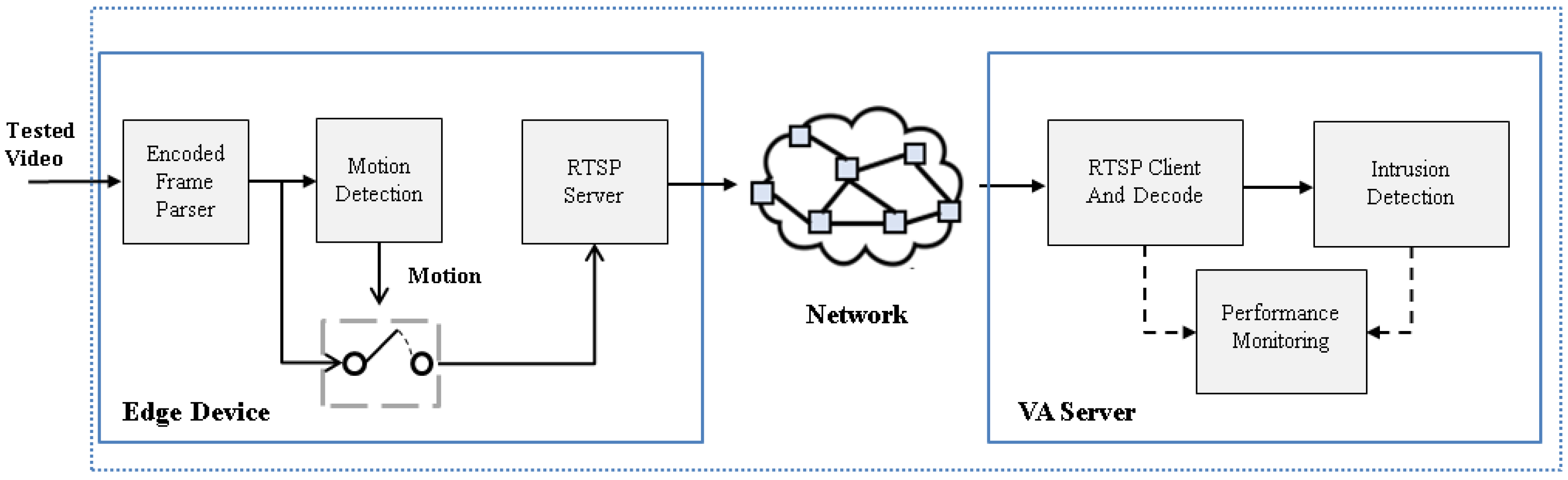
• Edge node implementation: The streaming data from the camera sources are parsed, and the proposed method is applied to detect moving objects in the current frame. If the encoded frame includes the motion, it will be forwarded to a cloud node using its own real-time streaming protocol (RTSP) server. To avoid decoding inaccuracies at the cloud node, all frames from the start time to the end time of the motion are continuously delivered in a connection session. Each session will start with an intra-coded frame.
• Cloud node implementation: receiving the forwarded encoded frame with the motion from the edge node over the network and then decoding and placing the output images into the intrusion detection module, which uses YOLO to detect humans.

4.1. Scenario Setup

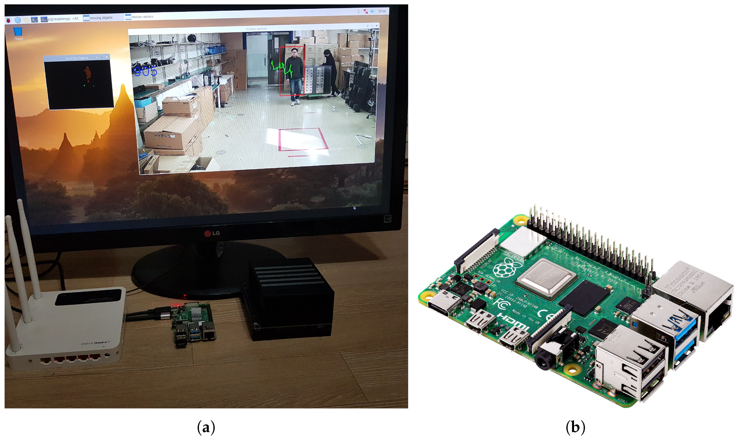
• Testbed: We built a testbed comprised of a single edge device node and a single video analytics server that runs as a cloud node, as shown in Figure 12. The edge device node involves the moving object detection and runs on a low computation device called the Raspberry Pi 4, and the video analytics server is executed on NVIDIA Jetson Xavier because it is a GPU that supports running YOLO. The hardware specifications of the edge node and video analytics server are listed in

  Table 1. Hardware specifications.

  Specifications	Edge Device	Video Analytics Server
  Device Name	Raspberry Pi 4	NVIDIA Jetson Xavier
  Operating System	Ubuntu 18.04, 64 bits	Ubuntu 18.04, 64 bits
  GPU	Not supported	NVIDIA Maxwell architecture with NVIDIA CUDA cores
  CPU	Quad-core ARM Cortext-A72	Quad-core ARM Cortext-A57 MPCore processor
  RAM	4 GB	8 GB

  . Note that the two devices are directly connected to a router using a wired cable.
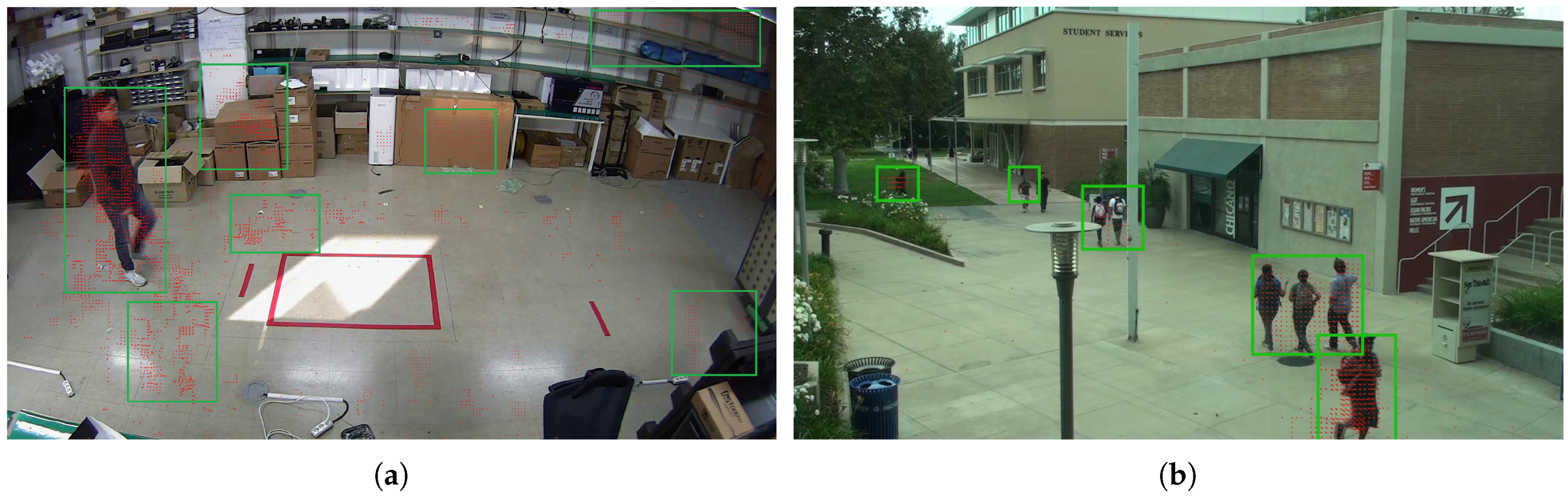
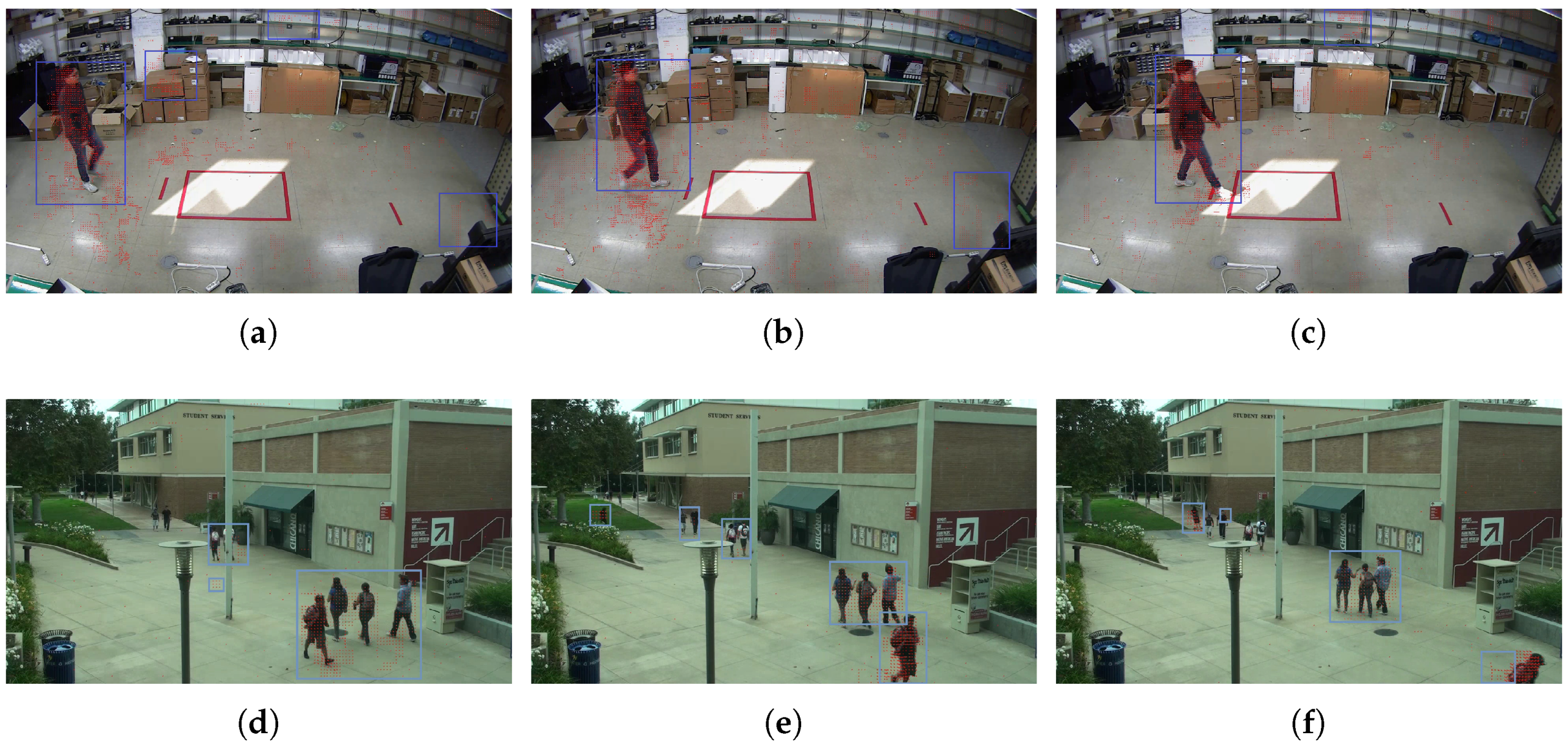
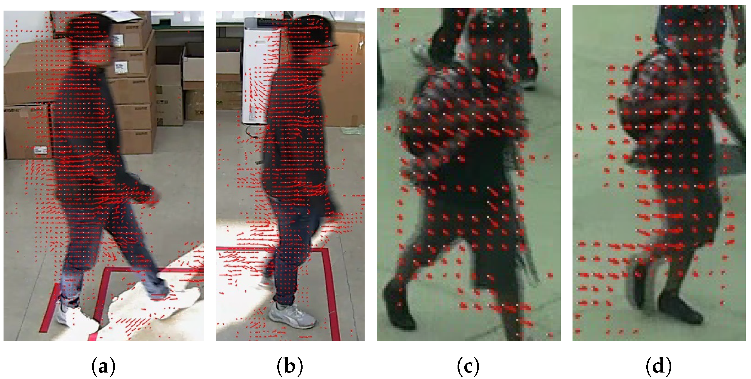
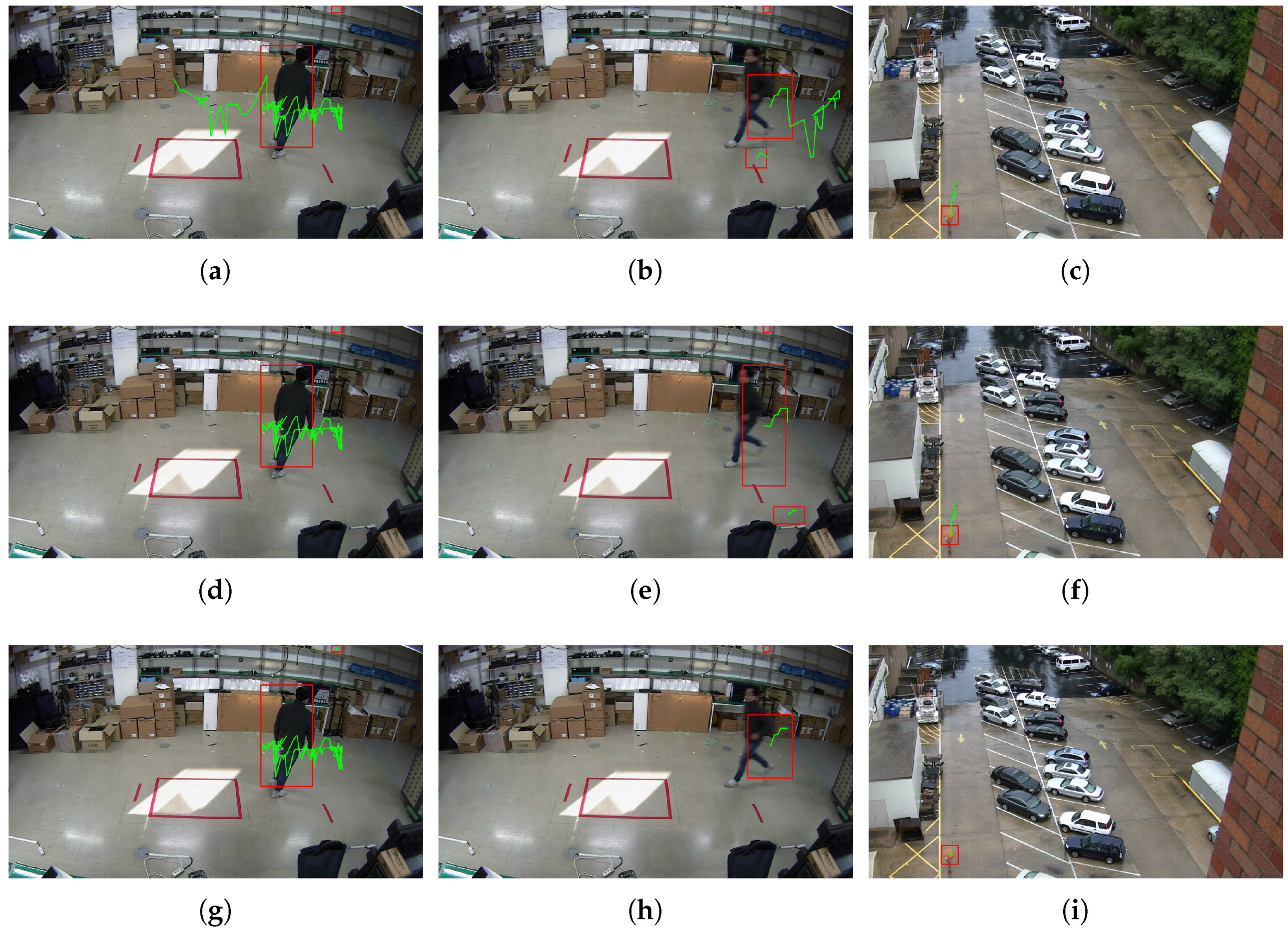
• Video test sequence: Experiments were conducted on the two video datasets. The VIRAT video dataset [42] was collected in natural scenes showing people performing normal actions for video surveillance domains. The second dataset was previously recorded from our surveillance camera and uploaded [43]. The details of our video test sequence and the ground-truth motion time are listed in

  Table 2. Video test sequence.

  Tested Video Information
  Resolution	1920 × 1080
  Length	6 min
  Codec	H264
  Group of picture (GOP)	30
  Frame rate	25

  and

  Table 3. Testbed: tested video ground-truth motion time.

  Time	Duration (Seconds)
  00:00:50 00:01:10	20
  00:01:25 00:01:45	20
  00:02:12 00:01:10	5
  00:02:39 00:02:45	6
  00:03:50 00:04:48	58
  00:05:00 00:05:35	35
  00:05:40 00:06:00	20
  Total	164

  .

We evaluate the performance of the moving object detection method and the proposed edge-to-cloud system separately.

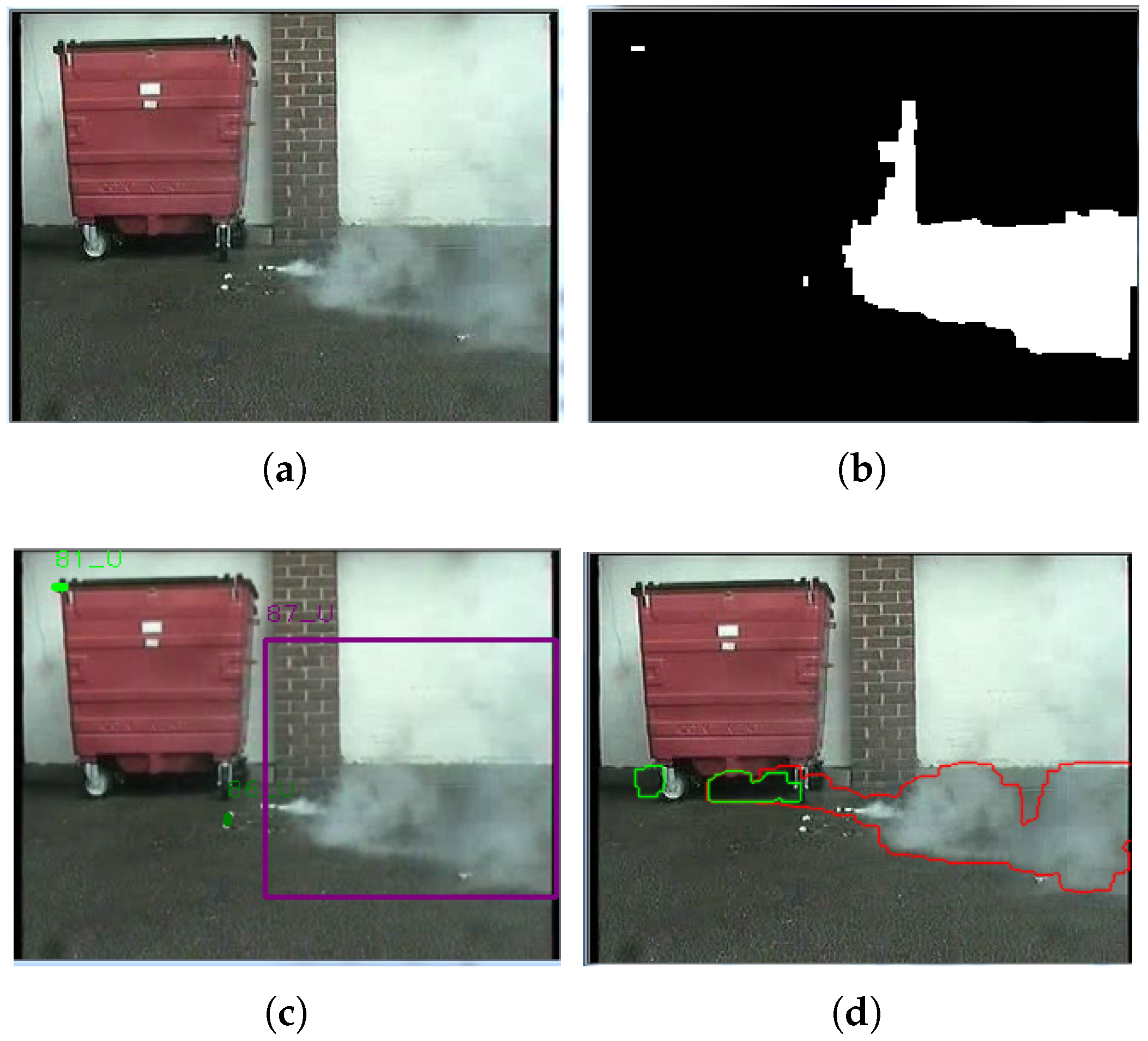
4.2. Light-weight Runtime Moving Object Detection in the Video Compressed-Domain

To evaluate the quality of the proposed method for the moving object detection, we calculated the IoU score metric of the detected object’s bounding box with those of the ground-truth bounding box. Because the accuracy of the proposed method depends on the MV’s density, we ran the proposed method multiple times with different scenario applications such as: different camera distances, different moving object speeds. We observed that except the I frame, which does not apply motion estimation, the moving objects including sometimes big MV noises always are detected in other frames. Example of the moving object detection results are shown in Figure 13.

The green bounding boxes shown in the figure are ground-truth bounding boxes, while the red bounding boxes are detected objects using the proposed method. The average IoU scores are shown in detail for each scenario in

Table 4. Average IoU of the moving object detection in the compressed-domain in different scenarios.

Video Test Sequence	Scenario		IoU Average
	Camera Position	Moving Speed
Our recorded test video	Near	Normal	0.75
Our recorded test video	Near	Fast	0.26
Video test from VIRAT	Far	Normal	0.6

. The results show that when a camera is placed at a close distance and the human does not move fast (i.e., human walking), the proposed method detected the human well and achieved a good average IoU score of 0.75. However, when the speed of the human was fast as in case of running or the camera was at a far distance, the MV’s density decreased, and the detector returned lower average IoU scores. For object tracking evaluation, the scenarios were run multiple times with different detection score thresholds $\alpha$ of 0.25, 0.4, and 0.5 with the results shown in Figure 14.

In this experiment, each $\alpha$ threshold was applied for the same three scenarios of human walking in Figure 14a,d,g, human running in Figure 14b,e,h, and the far camera distance in Figure 14c,f,i. We see that with each test scenario, with a lower $\alpha$ threshold value, the tracking object capability was better with longer object trajectories. However, it will increase the number of false alarm detections if the noisy MVs appear frequently in some specified areas.

To optimize the running time speed, as well as the performance, the edge node and cloud node were all implemented in C++ using the multithread architecture. We observed that the proposed method does not indicate additional computational difficulty and achieves the approved evaluated results in terms of processing time when compared with previous studies [15,16]. The average time consumption is measured with different video resolutions and shown in

Table 5. Average per-frame running times for the preprocessing and tracking procedures. Values are expressed in milliseconds (ms) and frames per second (FPS). ST-MRF, spatio-temporal Markov random field.

Frame Size	ST-MRF[16]	Graph Cuts[15]	Proposed Method
1280 × 720	64 ms (16 FPS)	62 ms (17 FPS)	39 ms (26 FPS)
1920 × 1080	N/A	N/A	69 ms (14 FPS)

. Compare to other studies, the average processing time for high definition resolution video is approximately 39 ms/frame, which outperforms most of the state-of-the-art methods. This indicates that the proposed algorithm almost handles the data in real-time.

4.3. Performance Evaluation Results

In this experiment, the proposed edge-to-cloud platform will be implemented and evaluated. Our recorded video test sequence is selected because it includes different moving object speeds. After experiments using different $\alpha$ in different scenarios, we found that the optimal $\alpha$ was 0.5 for this scenario. The entire demonstration was recorded and uploaded [44]. The evaluated performances of the demonstration are presented in detail as follows.

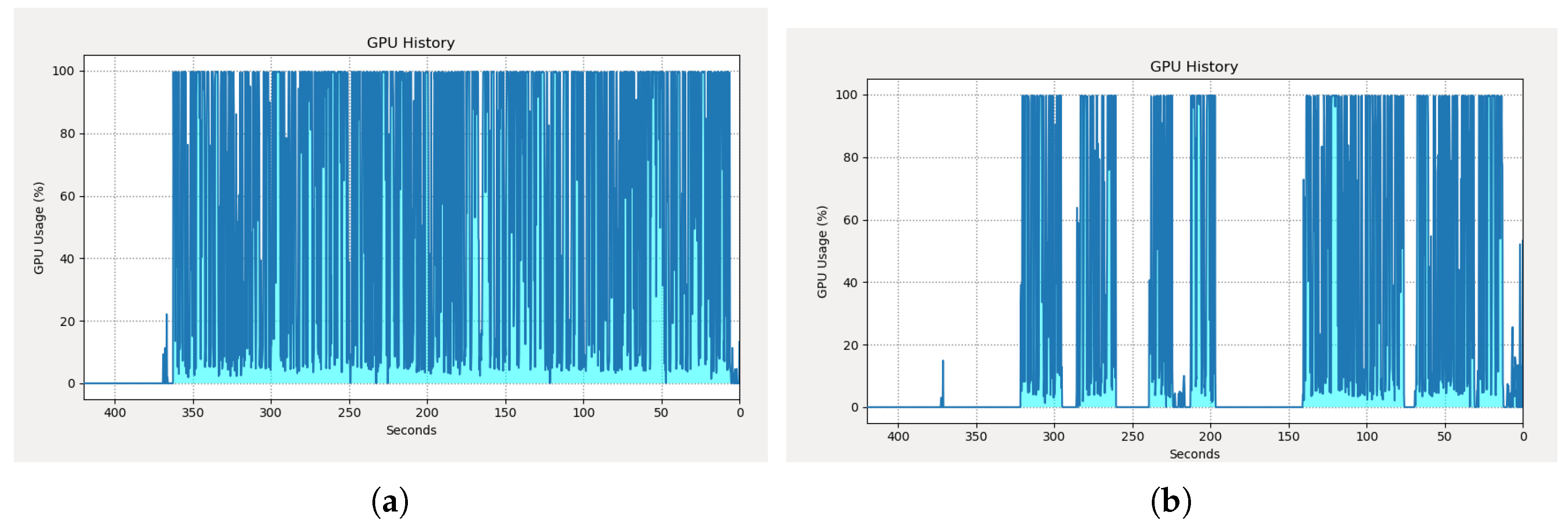
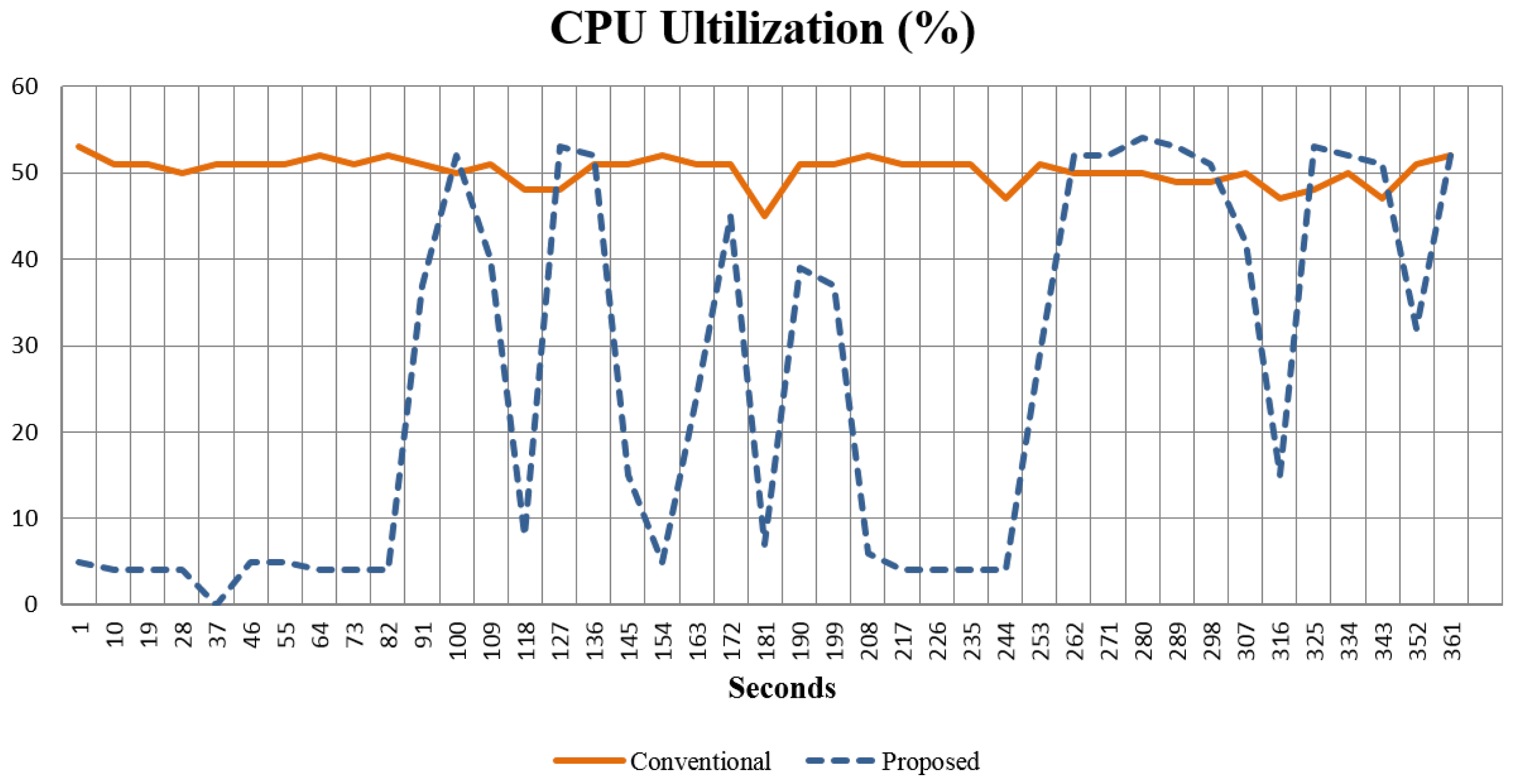
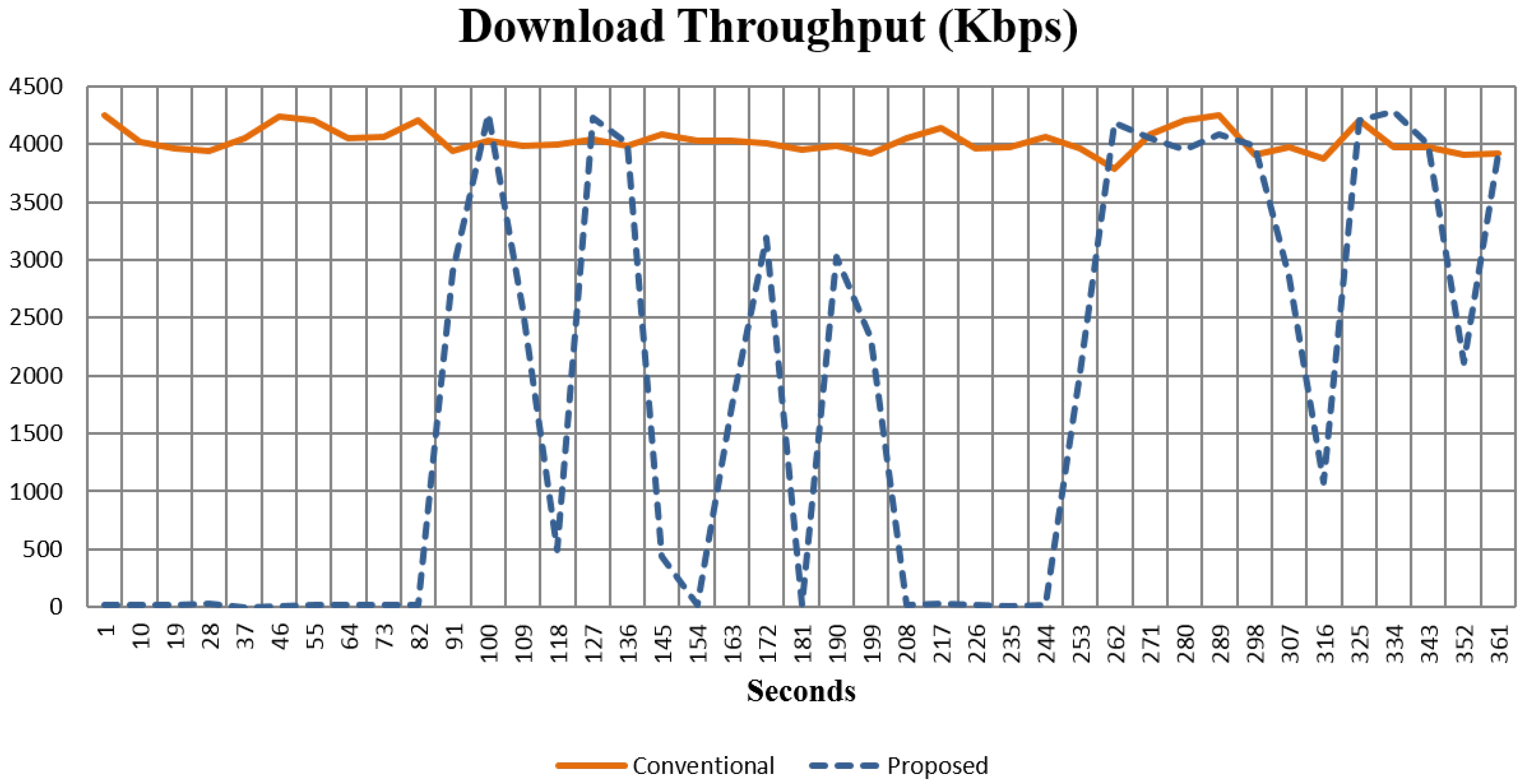
Computing Resource Consumption

During the demonstration of the intrusion detection application, the cloud node’s computing resources, including the CPU, GPU utilization, and network download throughput, were monitored and recorded and are shown in Figure 11. For comparison, the performance results are compared to those of the conventional method, which does not use the edge node, as shown in Figure 1. The results indicate that both methods achieve the same accuracy in terms of alert notification when humans entered the restricted area. The demonstration’s records of both these methods were uploaded to [45,46]. In terms of consumption of computational resources, the GPU, CPU utilization, and download throughput of both methods were measured and are presented in Figure 15, Figure 16 and Figure 17, respectively. The figures clearly show the advantage of using the proposed method. While the conventional method of processing all video frames captured from the camera leads to the consumption of computational resources, our method only processes when there is motion, and therefore, the computational resources are dynamically allocated and economical. Another observation is that our proposed method is extremely effective at detecting motion in the scene compared to the ground-truth motion time in Table 3. In detail, the time for consuming and releasing the computing resources of the VA server matches the time for the appearance and disappearance of motion in the ground-truth table. Since the conventional method processes all video frames, we assume that its computing resource average is S. According to the formulation (6), the performance ratio of both methods in this video will be as follows:

$$\frac{Com{p}_p}{Com{p}_c}=\frac{(K\times S+(N-K)\times T)}{N\times S}=\frac{K}{N}+(1-\frac{K}{N})\times \frac{T}{S}=\frac{140}{360}+(1-\frac{140}{360})\times \frac{T}{S}=0.4+0.6\times \frac{T}{S}$$

(10)

Compared with the performance ratio, which is calculated in the real scenario test in

Table 6. Average computing resources of both the conventional method and the proposed method.

Computing Resources	Conventional Method	Proposed Method	Performance Ratio
GPU Utilization (%)	65.61	33.73	0.51
CPU Utilization (%)	50.24	25.9	0.51
Download Throughput (Kbps)	4028	1808.2	0.45

, our performance theory model and real measurement match and are reasonable.

5. Conclusions

In this work, we propose an edge computing-based video analytics platform that utilizes the compressed-domain features at the edge device node to minimize the video data transfer of surveillance camera feeds to the video analytics server on the cloud. By exploiting the MVs from the compressed bitstream, edge devices can achieve a low processing complexity in the object-tracking task for surveillance videos. Based on the result of the moving object tracking, the edge device will consider whether the compressed frame should be forwarded to the cloud server. We implemented the proposed method including various computer vision algorithms such as video coding MV extraction, data clustering, and object tracking. The evaluation results show that the proposed method achieved the aims of the study and is fully compatible with cloud-based video analytics for surveillance systems without issues related to delay time or conflicts with other modules. Our implemented application is a light-weight edge-to-cloud platform that can be easily applied to other cloud-based video analytics application. In the future, we will continue to improve the video motion vector analysis method to recognize extremely small motions and reduce noise motions with higher accuracy.

References

1. Ananthanarayanan, G.; Bahl, V.; Cox, L.; Crown, A.; Nogbahi, S.; Shu, Y. Demo: Video Analytics-Killer App for Edge Computing. In ACM MobiSys; Association for Computing Machinery: Seoul, Korea, 2019. [Google Scholar]
2. Philippou, O. Video Surveillance Installed Base Report—2019. 2020. Available online: https://technology.informa.com/607069/video-surveillance-installed-base-report-2019 (accessed on 3 September 2020).
3. Stone, T.; Stone, N.; Jain, P.; Jiang, Y.; Kim, K.H.; Nelakuditi, S. Towards Scalable Video Analytics at the Edge. In Proceedings of the 2019 16th Annual IEEE International Conference on Sensing, Communication, and Networking (SECON), Boston, MA, USA, 10–13 June 2019; pp. 1–9. [Google Scholar]
4. Lu, X.; Izumi, T.; Takahashi, T.; Wang, L. Moving vehicle detection based on fuzzy background subtraction. In Proceedings of the 2014 IEEE International Conference on Fuzzy Systems (FUZZ-IEEE), Beijing, China, 20–24 August 2014; pp. 529–532. [Google Scholar]
5. Kumar, S.; Yadav, J.S. Segmentation of moving objects using background subtraction method in complex environments. Radioengineering 2016, 25, 399–408. [Google Scholar] [CrossRef]
6. Gujrathi, P.; Priya, R.A.; Malathi, P. Detecting moving object using background subtraction algorithm in FPGA. In Proceedings of the IEEE 2014 Fourth International Conference on Advances in Computing and Communications, Kerala, India, 27–29 August 2014; pp. 117–120. [Google Scholar]
7. Wang, Z.; Sun, X.; Diao, W.; Zhang, Y.; Yan, M.; Lan, L. Ground moving target indication based on optical flow in single-channel SAR. IEEE Geosci. Remote Sens. Lett. 2019, 16, 1051–1055. [Google Scholar] [CrossRef]
8. Favalli, L.; Mecocci, A.; Moschetti, F. Object tracking for retrieval applications in MPEG-2. IEEE Trans. Circuits Syst. Video Technol. 2000, 10, 427–432. [Google Scholar] [CrossRef] [Green Version]
9. Yoneyama, A.; Nakajima, Y.; Yanagihara, H.; Sugano, M. Moving object detection and identification from MPEG coded data. In Proceedings of the IEEE 1999 International Conference on Image Processing (Cat. 99CH36348), Piscataway, NJ, USA, 24–28 October 1999; Volume 2, pp. 934–938. [Google Scholar]
10. Dong, L.; Zoghlami, I.; Schwartz, S.C. Object tracking in compressed video with confidence measures. In Proceedings of the 2006 IEEE International Conference on Multimedia and Expo, Toronto, ON, Canada, 9–12 July 2006; pp. 753–756. [Google Scholar]
11. Achanta, R.; Kankanhalli, M.; Mulhem, P. Compressed domain object tracking for automatic indexing of objects in MPEG home video. In Proceedings of the IEEE International Conference on Multimedia and Expo, Lausanne, Switzerland, 26–29 August 2002; Volume 2, pp. 61–64. [Google Scholar]
12. Laroche, G.; Jung, J.; Pesquet-Popescu, B. RD optimized coding for motion vector predictor selection. IEEE Trans. Circuits Syst. Video Technol. 2008, 18, 1247–1257. [Google Scholar] [CrossRef]
13. Jiang, X.; Song, T.; Katayama, T.; Leu, J.S. Spatial Correlation-Based Motion-Vector Prediction for Video-Coding Efficiency Improvement. Symmetry 2019, 11, 129. [Google Scholar] [CrossRef] [Green Version]
14. Bross, B.; Helle, P.; Lakshman, H.; Ugur, K. Inter-picture prediction in HEVC. In High Efficiency Video Coding (HEVC); Springer: Berlin/Heidelberg, Germany, 2014; pp. 113–140. [Google Scholar]
15. Bombardelli, F.; Gül, S.; Becker, D.; Schmidt, M.; Hellge, C. Efficient Object Tracking in Compressed Video Streams with Graph Cuts. In Proceedings of the 2018 IEEE 20th International Workshop on Multimedia Signal Processing (MMSP), Vancouver, BC, Canada, 29–31 August 2018; pp. 1–6. [Google Scholar]
16. Khatoonabadi, S.H.; Bajic, I.V. Video object tracking in the compressed domain using spatio-temporal Markov random fields. IEEE Trans. Image Process. 2012, 22, 300–313. [Google Scholar] [CrossRef] [PubMed]
17. Boykov, Y.; Veksler, O.; Zabih, R. Fast approximate energy minimization via graph cuts. IEEE Trans. Pattern Anal. Mach. Intell. 2001, 23, 1222–1239. [Google Scholar] [CrossRef] [Green Version]
18. Zeng, D.; Zhu, M. Background subtraction using multiscale fully convolutional network. IEEE Access 2018, 6, 16010–16021. [Google Scholar] [CrossRef]
19. Chen, Y.; Wang, J.; Zhu, B.; Tang, M.; Lu, H. Pixel-wise deep sequence learning for moving object detection. IEEE Trans. Circuits Syst. Video Technol. 2017, 29, 2567–2579. [Google Scholar] [CrossRef]
20. Babaee, M.; Dinh, D.T.; Rigoll, G. A deep convolutional neural network for video sequence background subtraction. Pattern Recognit. 2018, 76, 635–649. [Google Scholar] [CrossRef]
21. Wang, Y.; Luo, Z.; Jodoin, P.M. Interactive deep learning method for segmenting moving objects. Pattern Recognit. Lett. 2017, 96, 66–75. [Google Scholar] [CrossRef]
22. Patil, P.W.; Murala, S. Msfgnet: A novel compact end-to-end deep network for moving object detection. IEEE Trans. Intell. Transp. Syst. 2018, 20, 4066–4077. [Google Scholar] [CrossRef]
23. Ou, X.; Yan, P.; Zhang, Y.; Tu, B.; Zhang, G.; Wu, J.; Li, W. Moving object detection method via ResNet-18 with encoder–decoder structure in complex scenes. IEEE Access 2019, 7, 108152–108160. [Google Scholar] [CrossRef]
24. Lee, J.; Park, M. An adaptive background subtraction method based on kernel density estimation. Sensors 2012, 12, 12279–12300. [Google Scholar] [CrossRef]
25. Stauffer, C.; Grimson, W.E.L. Adaptive background mixture models for real-time tracking. In Proceedings of the 1999 IEEE Computer Society Conference on Computer Vision and Pattern Recognition (Cat. No PR00149), Collins, CO, USA, 23–25 June 1999; Volume 2, pp. 246–252. [Google Scholar]
26. Lu, N.; Wang, J.; Wu, Q.; Yang, L. An Improved Motion Detection Method for Real-Time Surveillance. IAENG Int. J. Comput. Sci. 2008, 35, 1. [Google Scholar]
27. LeCun, Y.; Kavukcuoglu, K.; Farabet, C. Convolutional networks and applications in vision. In Proceedings of the 2010 IEEE International Symposium on Circuits and Systems, Paris, France, 30 May–2 June 2010; pp. 253–256. [Google Scholar]
28. Jarrett, K.; Kavukcuoglu, K.; Ranzato, M.A.; LeCun, Y. What is the best multi-stage architecture for object recognition? In Proceedings of the 2009 IEEE 12th International Conference on Computer Vision (ICCV), Kyoto, Japan, 29 September–2 October 2009; pp. 2146–2153. [Google Scholar]
29. Lee, H.; Grosse, R.; Ranganath, R.; Ng, A.Y. Convolutional deep belief networks for scalable unsupervised learning of hierarchical representations. In Proceedings of the ACM 26th Annual International Conference on Machine Learning, Montreal, QC, Canada, 14–18 June 2009; pp. 609–616. [Google Scholar]
30. Hussain, M.; Bird, J.J.; Faria, D.R. A Study on CNN Transfer Learning for Image Classification. In UK Workshop on Computational Intelligence; Springer: Berlin/Heidelberg, Germany, 2018; pp. 191–202. [Google Scholar]
31. Krizhevsky, A.; Hinton, G. Learning Multiple Layers of Features from Tiny Images; Technical Report; Citeseer: College Park, MD, USA, 2009. [Google Scholar]
32. Girshick, R.; Donahue, J.; Darrell, T.; Malik, J. Rich feature hierarchies for accurate object detection and semantic segmentation. In Proceedings of the IEEE Conference on Computer Vision and Pattern Recognition, Columbus, OH, USA, 23–28 June 2014; pp. 580–587. [Google Scholar]
33. Uijlings, J.R.; Van De Sande, K.E.; Gevers, T.; Smeulders, A.W. Selective search for object recognition. Int. J. Comput. Vis. 2013, 104, 154–171. [Google Scholar] [CrossRef] [Green Version]
34. Girshick, R. Fast r-cnn. In Proceedings of the IEEE International Conference on Computer Vision, Santiago, Chile, 7–13 December 2015; pp. 1440–1448. [Google Scholar]
35. Ren, S.; He, K.; Girshick, R.; Sun, J. Faster r-cnn: Towards real-time object detection with region proposal networks. In Advances in Neural Information Processing Systems; IEEE: Hoboken, NJ, USA, 2015; Volume 39, pp. 91–99. [Google Scholar]
36. Redmon, J.; Divvala, S.; Girshick, R.; Farhadi, A. You only look once: Unified, real-time object detection. In Proceedings of the IEEE Conference on Computer Vision and Pattern Recognition, Las Vegas, NV, USA, 27–30 June 2016; pp. 779–788. [Google Scholar]
37. Redmon, J.; Farhadi, A. Yolov3: An incremental improvement. arXiv, 2018; arXiv:1804.02767. [Google Scholar]
38. Liu, W.; Anguelov, D.; Erhan, D.; Szegedy, C.; Reed, S.; Fu, C.Y.; Berg, A.C. Ssd: Single shot multibox detector. In European Conference on Computer Vision; Springer: Berlin/Heidelberg, Germany, 2016; pp. 21–37. [Google Scholar]
39. Ester, M.; Kriegel, H.P.; Sander, J.; Xu, X. A density-based algorithm for discovering clusters in large spatial databases with noise. Kdd 1996, 96, 226–231. [Google Scholar]
40. Sheu, R.K.; Pardeshi, M.; Chen, L.C.; Yuan, S.M. STAM-CCF: Suspicious Tracking Across Multiple Camera Based on Correlation Filters. Sensors 2019, 19, 3016. [Google Scholar] [CrossRef] [PubMed] [Green Version]
41. Li, C.; Xing, Q.; Ma, Z. HKSiamFC: Visual-Tracking Framework Using Prior Information Provided by Staple and Kalman Filter. Sensors 2020, 20, 2137. [Google Scholar] [CrossRef] [PubMed] [Green Version]
42. The VIRAT Video Dataset. Available online: https://viratdata.org (accessed on 3 September 2020).
43. Recorded Video Test Sequence. Available online: https://youtu.be/v24ldT1AGRw (accessed on 3 September 2020).
44. Motion Vector Extraction Source Code. Available online: https://github.com/diennv/MotionVectorAnalysis (accessed on 3 September 2020).
45. The Conventional Method. Available online: https://www.youtube.com/watch?v=Cz_zxr_ElTU (accessed on 3 September 2020).
46. The Proposed Method. Available online: https://www.youtube.com/watch?v=-fRc36HAduI&feature=youtu.b (accessed on 3 September 2020).
Figure 1. Overview of the cloud-based video analytics server.
Applsci 10 06391 g001
Figure 2. Reference motion vectors in video coding.
Applsci 10 06391 g002
Figure 3. Example of motion vectors’ extraction. (a) Test video sequence from our recorded video. (b) Test video sequence from VIRAT.
Applsci 10 06391 g003
Figure 4. Smoke detection process: (a) input image, (b) foreground subtraction, (c) blob detection, and (d) smoke classification.
Applsci 10 06391 g004
Figure 5. Overview of the proposed edge-to-cloud system model.
Applsci 10 06391 g005
Figure 6. Workflow of the proposed detection-based tracking approach in the compressed-domain. MV, motion vector.
Applsci 10 06391 g006
Figure 7. Video coding motion vector extraction from consecutive frames with two video test sequences. (ac) our recorded video; (df) test video in VIRAT.
Applsci 10 06391 g007
Figure 8. Moving object detection by the proposed method with two different video test sequences: (a,e) MV extraction; (b,f) apply median filter; (c,g) clustering MVs; (d,h) blob detection.
Applsci 10 06391 g008
Figure 9. Motion vector of a moving object in different video test sequences: (a,b) our recorded video; (c,d) test video in VIRAT.
Applsci 10 06391 g009
Figure 10. Object matching method.
Applsci 10 06391 g010
Figure 11. Overview of the system design. RTSP, real-time streaming protocol.
Applsci 10 06391 g011
Figure 12. Testbed: (a) scenario setup, (b) the implemented edge device.
Applsci 10 06391 g012
Figure 13. Moving object detection by the proposed method in different scenarios: (ad) human walking; (eh) human running; (il) test with a far distance of the camera.
Applsci 10 06391 g013
Figure 14. Moving object tracking by the proposed method with different α thresholds: α = 0.25 in (ac), α = 0.4 in (df), and α = 0.5 in (gi).
Applsci 10 06391 g014
Figure 15. GPU monitoring: (a) with the conventional method; (b) with the proposed method.
Applsci 10 06391 g015
Figure 16. CPU monitoring with both the conventional method and the proposed method.
Applsci 10 06391 g016
Figure 17. Network download throughput monitoring with both the conventional method and the proposed method.
Applsci 10 06391 g017