Model Predictive Control of Grid Forming Converters with Enhanced Power Quality

Abstract

This paper proposes an enhanced finite control set model predictive control (FCS-MPC) strategy for voltage source converter (VSC) with a LC output filter. The proposed control scheme is based on tracking the voltage reference trajectory by using only a single-step prediction within the controller horizon. Besides, the suitability of different frequency control schemes with the proposed scheme to prevent from inherent variable switching behaviour of conventional FCS-MPC is investigated. Based on that, the proposed method targets two major factors influencing power quality in grid forming applications by enhancing the output voltage harmonic distortion and also preventing variable switching behaviour of FCS-MPC. Although compared to multi-step prediction approaches, only a single-step multi-objective cost function to improve computation efficiency is utilized, the introduced control schemes are able to deliver higher power quality compared to its counterpart methods as well. Furthermore, the effect of different applied cost functions on the transient response of the system is studied and investigated for the future use of the VSC in microgrids (MGs). The effectiveness of the proposed scheme was assessed by simulation using MATLAB/SIMULINK and experiment using a 5.5 kVA VSC module and the results were in good agreement.

1. Introduction

The concept of microgrids (MGs) has received considerable attention owing to its potential to serve as an alternative power source utilizing unconventional sources interfaced by the power converters, or supplying power to the critical loads in the main grid in case of networks failure [1]. Furthermore, MGs are an agglomeration of distributed energy systems, working in low-voltage, and provide heat or power or combined heat and power (CHP) to a particular area. MGs provide a platform to maximize reliability, availability, efficiency, security, and economic performance and can operate independently to isolate themselves from the main grid in case of faults. Based on the power converters operation, which are vital parts of MGs, they are classified into grid-following, grid-forming, and grid-supporting power converters [2,3]. The concept of a grid-forming power converter, as the main focus of this paper, is fundamental to the operation of a low-inertia power system dominated by non-rotational generation [4]. In such scenarios, grid-forming converters provide the frequency and voltage references for regulation purposes. Hence, they form the references for the other distributed generations (DGs) [5]. Moreover, grid-forming converters can be used in different cases such as parallel operation, grid-connected, and islanded modes, where grid-forming converters are supplied by stable power sources such as batteries, fuel cell modules, and turbines, as shown in Figure 1 [6]. Bearing in mind that connecting a large number of DGs to the grid will result in some difficulties in controlling the MGs system and therefore may cause severe problems in power quality, stability, reliability, and also security [7,8,9]. The negative impact generated by the agglomeration of the DGs in the MG entity can be resolved throughout applying some aspects such as optimized cooperation, advanced control strategies, and proper coordination [10]. In fact, providing a high power quality by using the grid forming converters is a very challenging process. Therefore, advanced control techniques have to be adopted in order to diminish the adverse effects caused by poor quality originators. The conventional way of realizing voltage source converter (VSC) control structure in the MGs is through hierarchical and organized linear control loops utilizing a pulse width modulator (PWM). Cascaded linear structure inherently introduces a low-pass filtering behaviour of the overall control system where the dominant time constant tends to rise by an order of magnitude with every loop. Moreover, as the converters usually have an LC filter installed at the output, there exists a dynamic coupling between the inductor current and capacitor voltage, which is cumbersome when cancelling it out due to the presence of computational and PWM delays.

In this paper, finite control set model predictive control (FCS-MPC) is used to control a stand-alone voltage source converter in order to form a voltage reference and regulate the frequency for the future use in MGs as a grid-forming type. FCS-MPC has been discussed intensively in [11,12,13,14,15,16] for grid-connected applications and [17,18,19] provide detailed discussions on the performance of different FCS-MPC algorithms. To sum up the detailed discussion in the references mentioned above, FCS-MPC enabled simplicity and ease of including the constraints and non-linearities, and it has been proposed to be applied in many applications such as electrical drives and grid-connected power electronic systems [20,21]. Mainly, these promising results were achieved because of the general concept of FCS-MPC, which is based on the principle of using a discrete model of the power converter with an associated filter to predict its future behaviour for all possible control inputs and, consequently, apply the one that minimizes a programmed cost function (CF) at every sampling time [17] (see Figure 2). The key idea is to use the raw processing power to embed all the inner control loops within a single algorithm that takes into account the model of the converter and its associated filter. This structure provides flexibility and inherent fast response and it has been addressed in [22,23] with a focus on balancing the power in between two parallel converters. Usually, CFs based on one step prediction/short-horizon become problematic when controlling higher-order plants (as in the case of a LC filter) due to the couplings between different state variables [24]. This problem has been solved in this paper by giving respect for all orders in order to decouple each variable and control it separately without a need for more computations compared to the computational burden in the long-horizon method [25,26]. That was done by proposing a solution, which explicitly deals with the dynamic coupling between the inductor current and capacitor voltage, allowing the usage of and one step prediction/horizon for effective voltage control of the converter associated with the LC filter. Besides, the conventional FCS-MPC has a problem of variable switching frequency [27], and this has led to some difficulties in the LC filter design resulting in low converter performance due to the use of an inappropriate filter. Thereby, high power losses are introduced by including an oversized filter [28]. Therefore, many research studies have been devoted to finding a feasible solution to obtain a fixed switching operation and facilitate the filter selection process [29,30]. The paper is structured as follows: the converter model and the proposed controller are described in Section 2. In Section 3, frequency control approaches are explained in detail. In Section 4, the obtained results and remarks to them are given. Finally, the summary of the work is described in Section 5. Novelty and contributions of this research are briefly summarized as follows:

• Propose a new term in the CF, resulting in less computation and higher power quality compared to the traditional schemes.
• Address the suitability of different frequency control strategies such as Simple Penalization (SP), Notch filter (N), and Periodic control (P) combined with the new improved algorithm (IMPC).
• Discusses the suitable size of LC filter that can be associated with the converter when the above-mentioned frequency control strategies are used with IMPC and CMPC algorithms.
• Address the proper selection of sampling time for all conventional (CMPC) and improved (IMPC) algorithms.
• Shed light on many aspects such as spectrum analysis, steady-state operation, transient operation, power quality and factors tuning for eight different predictive schemes such as CMPC, IMPC, SP-CMPC, SP-IMPC, N-CMPC, N-IMPC, P-CMPC, and P-IMPC.

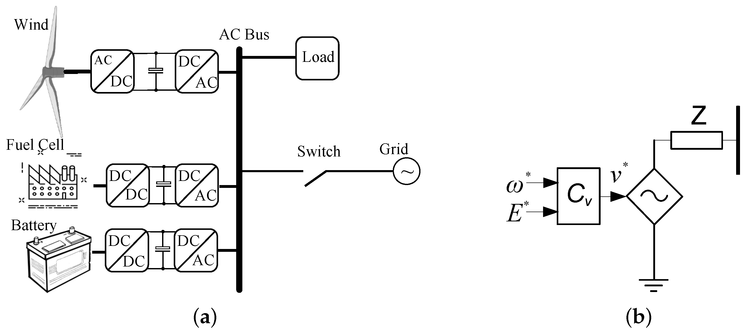
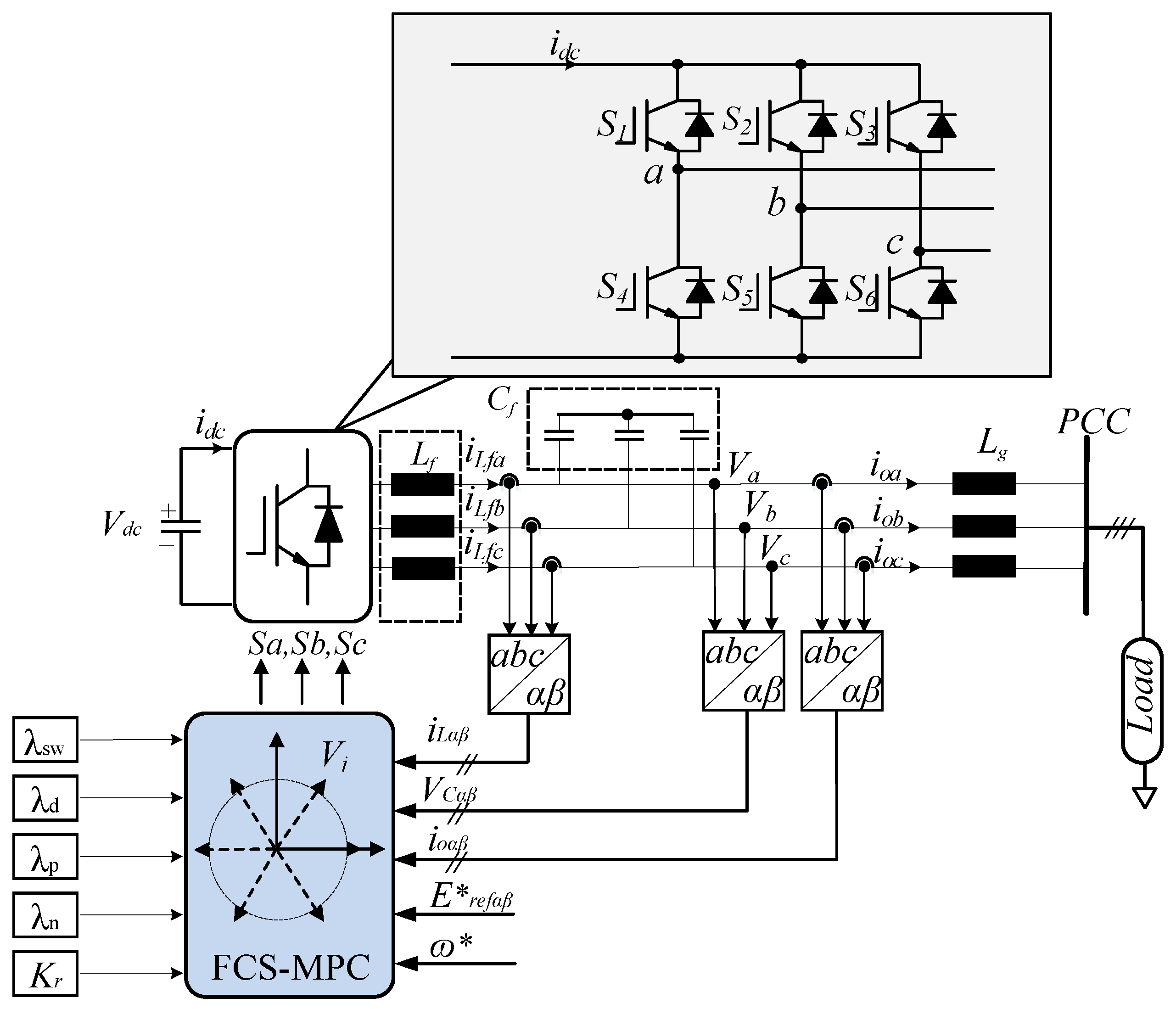
2. Converter Model and System Description

2.1. Converter Model

Figure 2 shows the circuit schematic of a two-level three-phase VSC. The power switches in each leg operate in a complementary mode. The switching states can be represented by the switching signals $S_{ka}$, $S_{kb}$, and $S_{kc}$, which are defined as follows:

$$S_{ka}=\left\{\begin{array}{c}1 \mathrm{if} S_1 \mathrm{on} \mathrm{and} S_4 \mathrm{off}\\ 0 \mathrm{if} S_1 \mathrm{off} \mathrm{and} S_4 \mathrm{on}\end{array}\right.$$

(1)

$$S_{kb}=\left\{\begin{array}{c}1 \mathrm{if} S_2 \mathrm{on} \mathrm{and} S_5 \mathrm{off}\\ 0 \mathrm{if} S_2 \mathrm{off} \mathrm{and} S_5 \mathrm{on}\end{array}\right.$$

(2)

$$S_{kc}=\left\{\begin{array}{c}1 \mathrm{if} S_3 \mathrm{on} \mathrm{and} S_6 \mathrm{off}\\ 0 \mathrm{if} S_3 \mathrm{off} \mathrm{and} S_6 \mathrm{on}\end{array}\right.$$

(3)

The filter inductance equation can be expressed in the vectorial form as:

$$L_f\frac{\mathrm{d}{i}_{L_f}}{\mathrm{d}t}=V_i-V_{c_f}$$

(4)

where $L_f$ is the filter inductance ($L_a$, $L_b$, $L_c$). The equation that describes the dynamic behaviour of the output voltage can be expressed mathematically as:

$$C_f\frac{\mathrm{d}{V}_{c_f}}{\mathrm{d}t}=i_{L_f}-i_o$$

(5)

where $C_f$ is the filter capacitance ($C_a$, $C_b$, $C_c$). These equations can be rewritten in the state space model as:

$$\frac{\mathrm{d}x}{\mathrm{d}t}=Ax+B{V}_i+B_2{i}_o$$

(6)

where,

$$x=\left[\begin{array}{c}{i}_{L_f}\\ V_{c_f}\end{array}\right]$$

(7)

$$A=\left[\begin{array}{cc}-R_f/L_f& -1/L_f\\ 1/C_f& 0\end{array}\right]$$

(8)

$$B=\left[\begin{array}{c}1/L_f\\ 0\end{array}\right]$$

(9)

$$B_2=\left[\begin{array}{c}0\\ -1/C_f\end{array}\right]$$

(10)

where $i_{Lf}$ and $V_{cf}$ are the filter current and voltage respectively. $i_o$ is the load current, which can be estimated or measured. In this paper, $i_o$, $i_{Lf}$, and $V_{cf}$ are measured and transformed to the alfa-beta reference frame within the state space model. $V_i$ is the inverter voltage of the system, and it has eight different voltage vectors, as shown in Figure 3. More details for the state-space model derivation and discretization method are presented in [31]. A discrete model is obtained from (6), and it can be expressed as follows:

$$x\left(\begin{array}{c}k+1\end{array}\right)=A_{q}x\left(\begin{array}{c}k\end{array}\right)+B_q{v}_i\left(\begin{array}{c}k\end{array}\right)+B_{dq}{i}_o\left(\begin{array}{c}k\end{array}\right)$$

(11)

where,

$$A_q=ex{p}^{A{T}_s}$$

(12)

$$B_q{=}_0^{T_s}ex{p}^{A\tau }Bd\tau$$

(13)

$$B_{dq}{=}_0^{T_s}ex{p}^{A\tau }{B}_{d}d\tau$$

(14)

where $T_s$ is the sampling time. This model is used to predict the filter voltages and currents for every possible input voltage. The selection of the optimal input voltage depends on the CF. In the next subsections, the conventional FCS-MPC algorithm and the proposed one will be discussed.

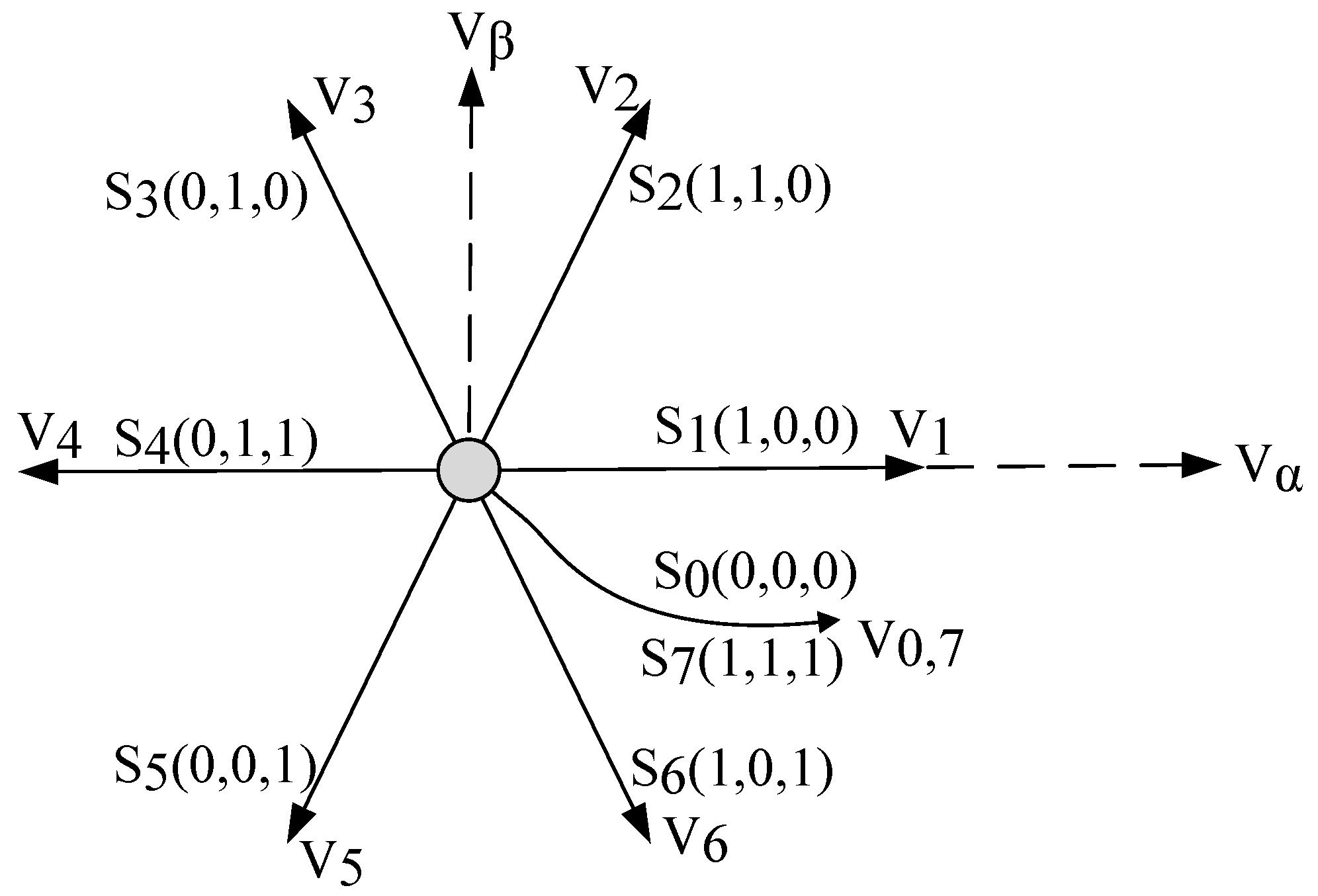
2.2. Conventional FCS-MPC Scheme for Voltage Regulation

Figure 2 shows a block diagram of a three-phase VSC based on a FCS-MPC algorithm. In its basic form, the algorithm is executed sequentially, and at the beginning of each sample, it applies the switching configuration, which is calculated in the previous calculation step. Then, it receives the measurements and selects the new switching configurations accordingly and apply them at the next instant. The following CF is implemented in a stationary reference frame ($\alpha -\beta$):

$$\begin{array}{c}\hfill g={(V_{re{f}_{\alpha }}^{*}-V_{c_{f\alpha }}^p(k+1))}^2+{(V_{re{f}_{\beta }}^{*}-V_{c_{f\beta }}^p(k+1))}^2\end{array}$$

(15)

where g is the CF, $V_{re{f}_{\alpha }}^{*}$ and $V_{re{f}_{\beta }}^{*}$ are the real and imaginary components of voltage reference signals in the stationary reference frame, while $V_{c_{f\alpha }}^p(k+1)$ and $V_{c_{f\beta }}^p(k+1)$ are the predicted components for each possible switch configuration. The conventional CF, as in Equation (15), uses a regulation strategy, which results in a minimal magnitude error at the next sampling instance. In first order plants, the variable of interest is directly regulated by the control input, allowing an instantaneous change of its derivative at a particular sampling instance. Hence, looking further than one prediction step ahead is optimal only for the first order plants [25]. For second order plants, capacitor voltage in the LC filter configuration is regulated indirectly through the inductor current. As the respective current cannot change its value instantaneously, the capacitor cannot change its derivative instantaneously. Therefore, no respect is given to the capacitor voltage derivative, which determines the heading of its trajectory. There are two possibilities to improve the power quality of the discussed configuration. Firstly, by applying a two-step or three-step prediction strategy, but using this approach makes the computations too intensive for practical applications. The other possibility evaluates for one prediction step by assuming that the same configuration will be kept for the next two periods $(k+2)$ in advance. This approach requires a highly accurate model of the system and it does not consider the capacitor voltage trajectory during inter-sampling periods [18,19].

2.3. Proposed FCS-MPC Scheme

Using the voltage reference track as the only objective in the grid-forming converter is inadequate with a second order plant. Therefore, in order to improve the capacitor voltage quality, an improved CF is discussed here. As discussed in the previous subsection, the inability to control the derivative of capacitor voltage is a fundamental cause of high THDv. Therefore, the ideal regulator should track both the voltage reference and its derivative simultaneously, which can be included as two signals treated as two separate references as follows:

$$V_{c_f}^{*}\left(t\right)=V_{ref}^{*}sin\left({\omega }_{ref}t\right)+j{V}_{ref}^{*}cos\left({\omega }_{ref}t\right)$$

(16)

where $V_{ref}^{*}$ and ${\omega }_{ref}$ are the amplitude and frequency of the reference signal, respectively. The voltage derivative reference is obtained as follows:

$$\frac{d{V}_{c_f}^{*}\left(t\right)}{dt}={\omega }_{ref}{V}_{ref}^{*}cos\left({\omega }_{ref}t\right)-j{\omega }_{ref}{V}_{ref}^{*}sin\left({\omega }_{ref}t\right)$$

(17)

Tracking of $V_{c_f}^{*}\left(t\right)$ is already accomplished by the presented CF in Equation (15). Therefore, what remains is to design a CF, which ensures that $\frac{d{V}_c\left(t\right)}{dt}$ tracks $\frac{d{V}_c^{*}\left(t\right)}{dt}$. In order to ensure that the voltage derivative tracks the reference, the predicted value is needed and can be taken from the predicted currents, which are calculated directly from the discrete model of the converter:

$$\frac{d{V}_{c_f}\left(t\right)}{dt}=\frac{i_{L\alpha }\left(t\right)-i_{o\alpha }\left(t\right)}{C_f}+j\frac{i_{L\beta }\left(t\right)-i_{o\beta }\left(t\right)}{C_f}$$

(18)

It can be seen that the voltage derivative trajectory will be well tracked if the respective differences between the first and second term from Equations (17) and (18) are minimized. These equations are explicitly formulated as the following CF:

$$\begin{array}{cc}\hfill g_I& ={(I_{f\alpha }(k+1)-I_{o\alpha }\left(k\right)+C_f{\omega }_{ref}(V_{ref\beta }^{*}\left(k\right)))}^2+{(I_{f\beta }(k+1)-I_{o\beta }\left(k\right)+C_f{\omega }_{ref}(V_{ref\alpha }^{*}\left(k\right)))}^2\hfill \end{array}$$

(19)

The term $g_I$ can now be added to the conventional CF in Equation (20), and the weight ${\lambda }_d$ controls its effect:

$$\begin{array}{cc}\hfill g& ={(V_{re{f}_{\alpha }}^{*}-V_{c_{f\alpha }}^p(k+1))}^2+{(V_{re{f}_{\beta }}^{*}-V_{c_{f\beta }}^p(k+1))}^2+({\lambda }_d*g_I)\hfill \end{array}$$

(20)

As introduced in this paper, another contribution is to find out the suitability of the frequency control techniques with both conventional and improved CFs. Therefore, in the next section, three different frequency control techniques such as, simple penalization (SP) control, Notch (N) control and Periodic (P) control will be discussed and redesigned in order to be incorporated with the improved and conventional CFs as well.

3. Frequency Control

The FCS-MPC algorithm decides the optimal states to minimize the voltage error, that is given in every sample, but it leads to random commutations, resulting in no control over the switching frequency for any time span. This may lead to introduce some losses, electromagnetic interference, resonances, and unbalanced stresses on the switches. In order to control the switching frequency through a single CF using the FCS-MPC, the algorithm should comply with some requirements such as reference tracking, computation time, simplicity, and flexibility. In the same time, all objectives should be regulated without hindering each other. In the case of initiating frequency control, it is important to have controllable objectives, which could be equal or unequal, in term of importance, to the proposed derivative term in order to achieve good power quality. That can be done by designing the weighting factors of each objective in the whole CF. Thus, in the discussed FCS-MPC strategy here, the CF should regulate the switching frequency, not at the expense of the other objectives or at least with a minimum impact. Thereby, if a control objective overwhelms the others, the controller will only care about minimizing the considered objective, fading the other objectives or making them less important. In this context, a detailed explanation for the improved CFs using different frequency control techniques of simple penalization (SP), Notch (N) and Periodic (P) will be given in the next subsections.

In this paper, the improvement is based on tracking the capacitor current, and including it in the main CF as a secondary objective in order to control its importance by a factor ${\lambda }_d$. Accordingly, the predictive schemes in Equations (27)–(29), should guarantee the optimum operation without introducing any conflicts between the other objectives which is leading to a degradation in the controller performance. The controllers damping ability, derivative term, has been tested at 2 kHz, which is the concentrated switching frequency, and that is relatively higher than the resonance frequency. The idea is to test all kind of studied CFs at the same conditions. Furthermore, the physical filter values LC, as introduced in

Table 1. Filter design parameters for the simulation and experimental setup.

Parameter	5.5 kVA System (Experimental)	System Model (Simulation)
S	5.5 kVA	5.5 kVA
$V_o$	230	230
$V_{dc}$	600	600
$\Delta$ I	$10\%$	$10\%$
$Q_c$	<$5\%S$	<$5\%S$
$f_g$	50 Hz	50 Hz
$Z_{Rd}$	$X_{Cf}$(${\omega }_r$)	$X_{Cf}$(${\omega }_r$)
$f_{res}$	10 $f_s$<$f_r$<1/2 $f_s$	10 $f_s$<$f_r$<1/2 $f_s$
$f_s$	40 kHz	-40 kHz in order to com- apare with the experimental (Ts = 25 μs) -80 kHz in order to show the sampling effects (Ts = 12.5 μs)
$L_f$	5 mH	-For 80 kHz = 2.5 mH -For 40 kHz = 5 mH
$C_f$	60 μF	-For 80 kHz = 20 μF -For 40 kHz = 60 μF

, were available in the laboratory for experimental validations.

3.1. Simple Penalization

A basic strategy to regulate the switching frequency is to penalize the act of commutation, which can be controlled by the ${\lambda }_{sw}$ and yield to:

$$\Delta S_k={\lambda }_{sw}{\left(S_k-S_{k-1}\right)}^2$$

(21)

When adding Equation (21), which illustrates the simple penalization frequency control technique (SP) to the conventional or improved CFs, the switching frequency is controlled. In case the voltage or its derivative has a large error, its corresponding value in the cost function would be large enough to overcome the penalization during the switching. Thus, strong importance should be given to the penalization term by setting the value of ${\lambda }_{sw}$ high, then the commutation of the last step will be maintained to provide switching’s reduction. Figure 4 shows the relative importance of the penalization term with the voltage tracking term. This strategy leads to a lower average frequency and higher voltage error, as shown in Figure 5. Considering that the spectrum will still spread in a wide band range and concentrated more to the lower frequencies. Later on, in the results and discussion section, the weighting factor design for both SP-CMPC and SP-IMPC will be discussed.

3.2. Notch Filter

The aforementioned strategy focuses on the reduction of the switching while this strategy aims to concentrate the voltage spectrum around the desired frequency by utilizing a digital notch filter. Generally, notch filters are shaping the spectrum at certain frequencies, where they need different weight values, to allow control of harmonics. The notch filter is designed for the IMPC scheme in order to control the switching frequency of the grid-forming converter. The implementation of the notch filter is done using the discrete-time domain. Therefore, the CF can be modified as:

$$g_{m1}={\lambda }_n{F}_n\left(g\right)$$

(22)

where ${\lambda }_n$ is the weighting factor and $F_n$ is the second-order band-stop filter. A Tustin discretization of the notch filter is considered in the filter design. Similarly, the derivative term $g_I$ in Equation (19) can be modified as:

$$g_{m2}={\lambda }_n{F}_n\left(g_I\right)$$

(23)

The implemented notch filter in this paper, which has a frequency concentration at 2 kHz is illustrated in Equation (24):

$${\mathbf{H}}_{2kH}=\frac{0.9849z^2-1.875z+0.9849}{z^2-1.875z+0.9698}$$

(24)

Notably, changing the filter bandwidth gives a different spreading range around the desired frequency. Similarly to the SP controller, the weighting factor design for both N-CMPC and N-IMPC will be discussed in the results and discussion section.

3.3. Periodic Control

The periodic control strategy focuses on fixing the time it takes for two consecutive similar commutations [32]. It means that any two ups or downs, same direction, form a similar commutation. The objective is to control the $T_{up}$ and $T_{down}$. The key idea is to achieve a modulation behaviour similar to the PWM pattern.

In periodic control, the switching frequency is compared with a reference time $T_r$, which is used for both up and down events in order to achieve the desired performance by applying the states, which are minimizing the error. The cost function, which is given in Equation (25) shows how the up and down events can be evaluated in order to regulate the switching frequency as follows:

$$g_p={\lambda }_p({(T_{up}-T_r)}^2+{(T_{down}-T_r)}^2)$$

(25)

where it can be rewritten as the following in the discrete form:

$$g_p={\lambda }_p({(K_{up}-K_r)}^2{T}_s^2+{(K_{down}-K_r)}^2{T}_s^2).$$

(26)

The algorithm predicts the state of $K_{up}=\frac{T_{up}}{T_s}$ and $K_{down}=\frac{T_{down}}{T_s}$ for all possible states, which are eight states in the case of the VSC. It is worth to mention that $K_r=\frac{f_s}{f_r}$ is the reference frequency that is given to the MPC controller to reshape the spectrum around the frequency of interest and its multiples. The factor ${\lambda }_p$ is used to mitigate the deviation as long as the stability of the overall system is preserved. The complete CFs of the conventional (P-CMPC) and improved (P-IMPC) periodic schemes are calculated in Equation (29).

$$g_s=\stackrel{SP-IMPC}{\overbrace{\stackrel{SP-CMPC}{\overbrace{g+{\lambda }_{sw}{\left(S_k-S_{k-1}\right)}^2}}+g_I}}$$

(27)

$$g_n=\stackrel{N-IMPC}{\overbrace{\stackrel{N-CMPC}{\overbrace{g+{\lambda }_n{F}_n{(V_{ref}-V_{cf})}^2}}+g_I+{\lambda }_n{F}_n\left(g_I\right)}}$$

(28)

$$g_p=\stackrel{P-IMPC}{\overbrace{\stackrel{P-CMPC}{\overbrace{g+{\lambda }_p({(K_{up}-K_r)}^2{T}_s^2+{(K_{down}-K_r)}^2{T}_s^2)}}+g_I}}$$

(29)

4. Results and Discussion

All discussed predictive control algorithms were implemented using the dSpace with DS 1007 power dual-core 2 GHz processor board. A flow chart showing the implementation steps of all algorithms can be found in Figure 6. The maximum achieved turn around time was around 22 μs. It should be noted that 9 μs was introduced by the auxiliary tasks (A/D conversion). In order to reduce the time taken by the A/D, an observer could be used to estimate the load current instead of measuring it. Since the dSpace A/D samples at a rate of 1 MS/s, that will save 3 μs from the total needed time. Moreover, the computational delay of exact Ts is compensated as discussed in [33]. The overall parameter of the test setup and simulation model can be seen in Table 1, and the setup is shown in Figure 7. Due to the setup limitation, both the simulation model and the setup have been operating at a 40 kHz sampling frequency. In order to illustrate the effect of different samplings, simulation results, in which the sampling is 80 kHz, are provided. FCS-MPCs based on the periodic, notch, penalization control algorithms have been verified experimentally, where a 5.5 kW rated power system has been built for that purpose. The power stage comprises a delta-star transformer to provide the DC-link voltage through an input filter to a rectifier. A two-level three-phase VSC (Danfoss type), the LC filter on the converter side, is loaded with a linear load. It should be noted that the Danfoss VSC contains electrolytic DC-link capacitor. In this work, the LC filter design was based on choosing low resonance frequency, as shown in Figure 8, to verify and make the FCS-MPC algorithms feasible for the study. As future work, each algorithm should have its optimized filter design, which will be briefly summarized later in the end of this paper.

4.1. Spectrum Analysis

The spectrum analysis is shown in this work in order to validate the functionality of the proposed FCS-MPC algorithms, where several points have been observed during the tests as follows:

□

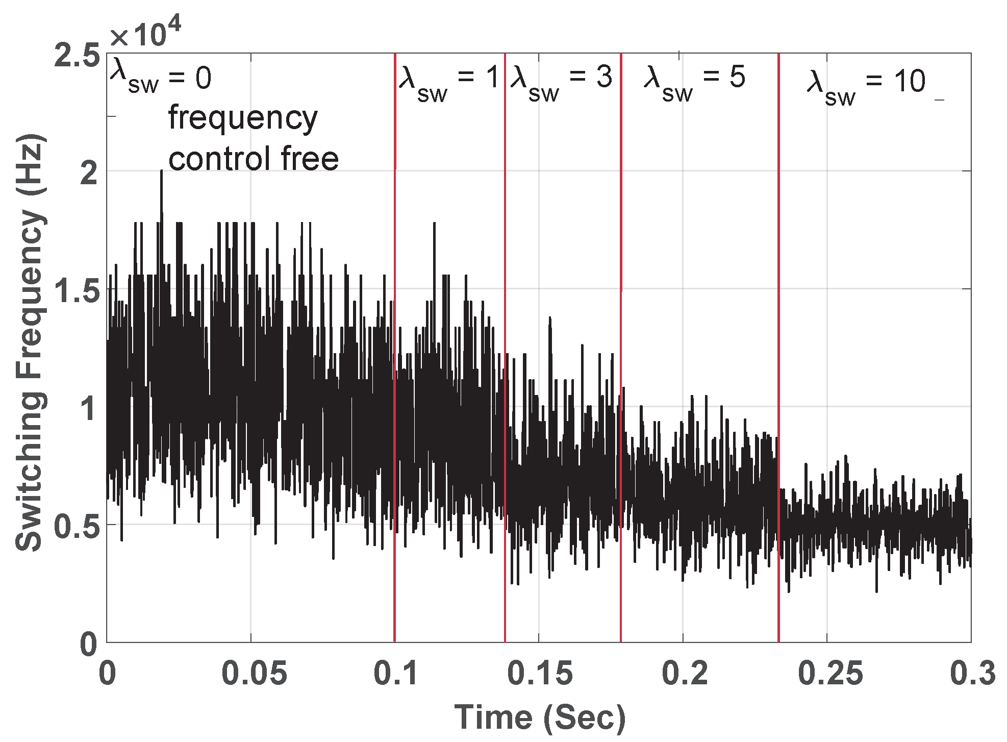
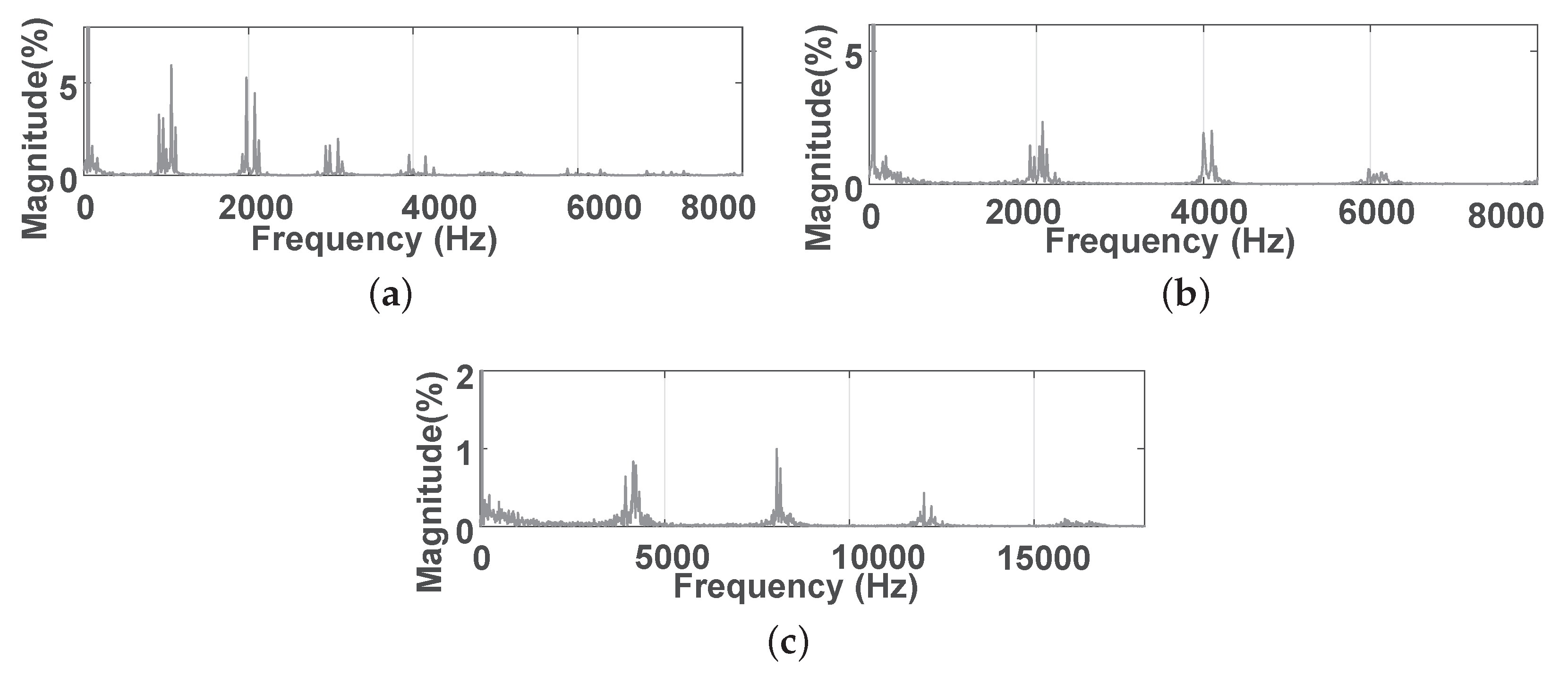
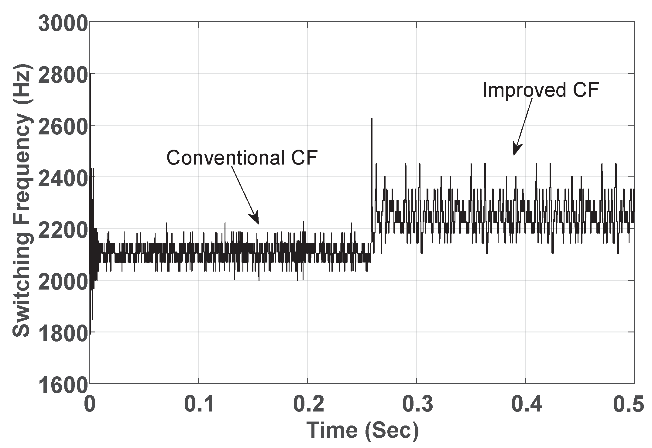
In Figure 9, the switching frequency fixed behaviour is obtained successfully by the periodic control technique. In case of having no control over the switching frequency, both conventional and improved FCS-MPC have high switching fluctuations. Thus, the output voltage and current harmonics are spread to a wide range of frequencies, as shown in Figure 10.

□

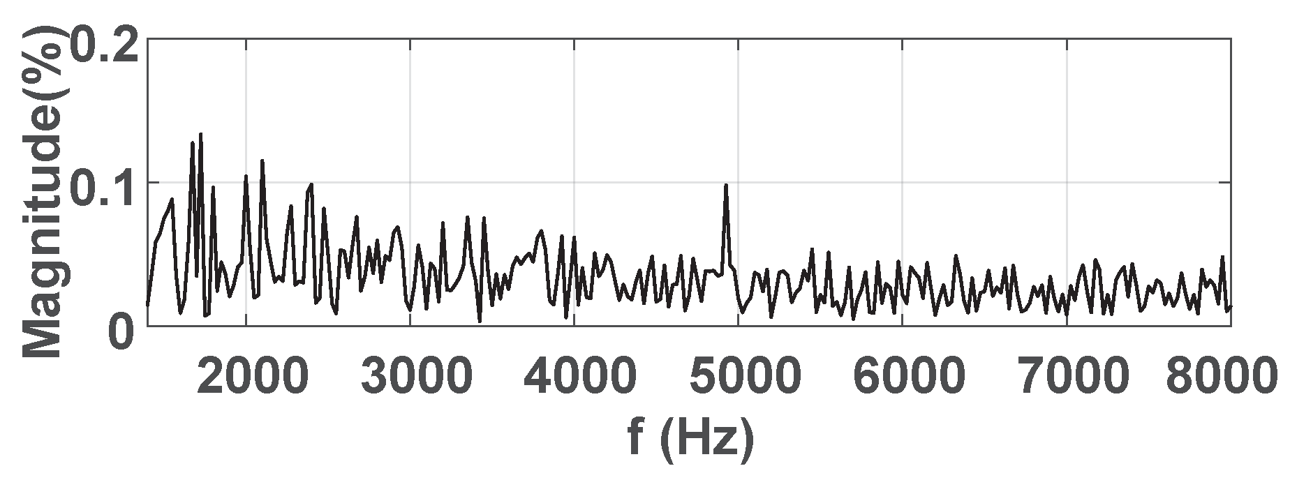
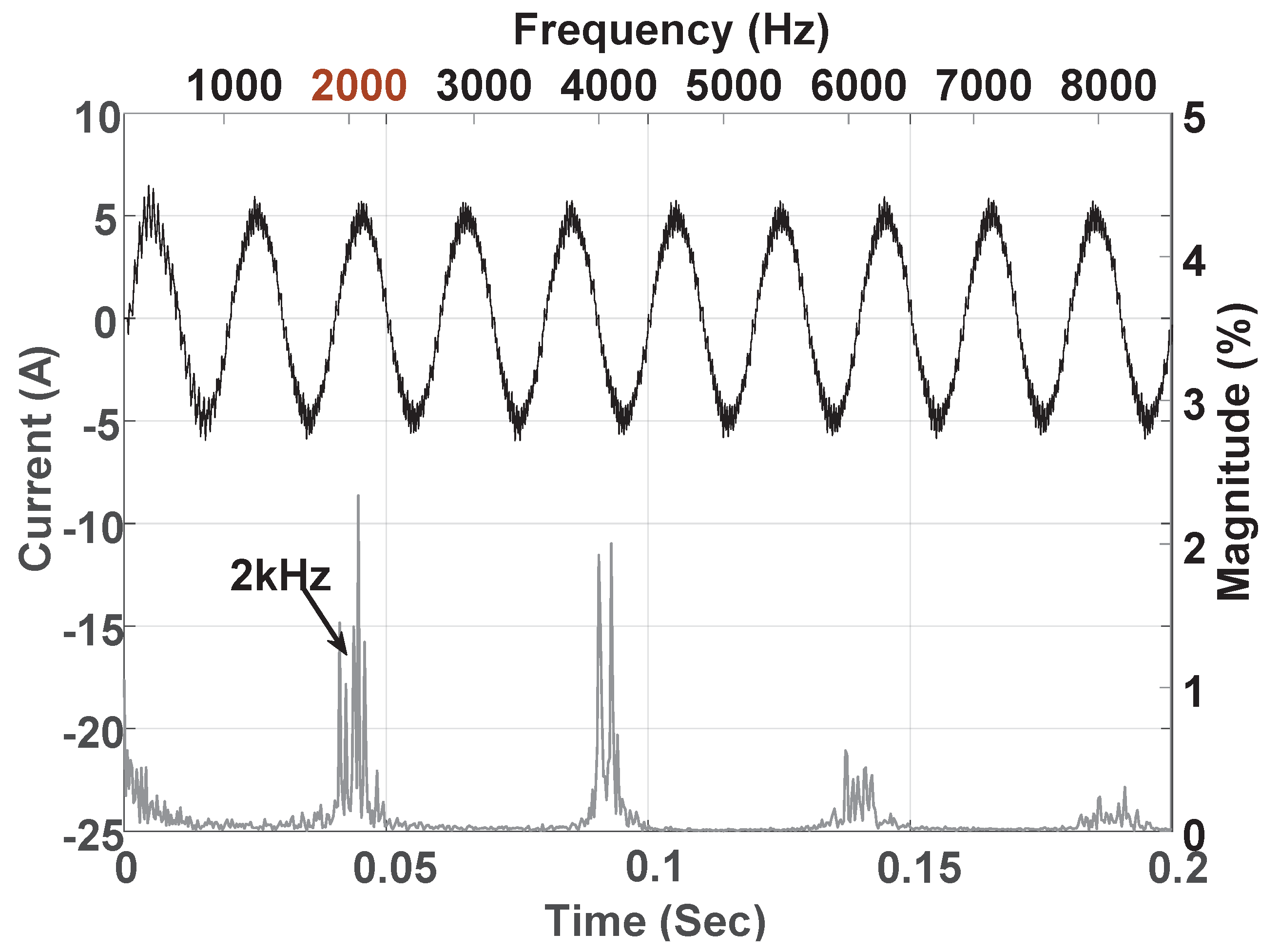
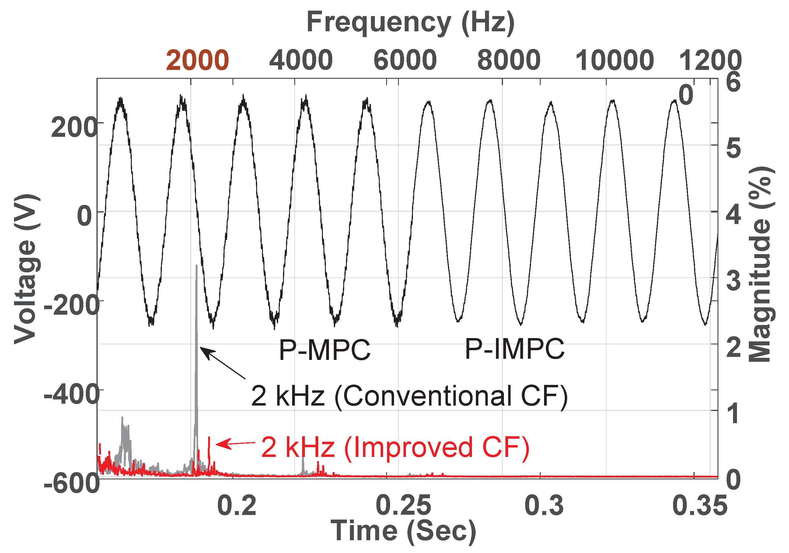
Figure 11 shows the output current spectrum on phase (a) following a reference frequency of 2 kHz using P-CMPC strategy. Here, it can be seen clearly that the output spectrum presents a similar behaviour as the one achieved with using a modulator. In Figure 12, P-IMPC has a magnitude’s reduction in the output spectrum, which is resulting in a higher power quality than the P-CMPC as it is shown in the time between 0.26 s and 0.36 s.

□

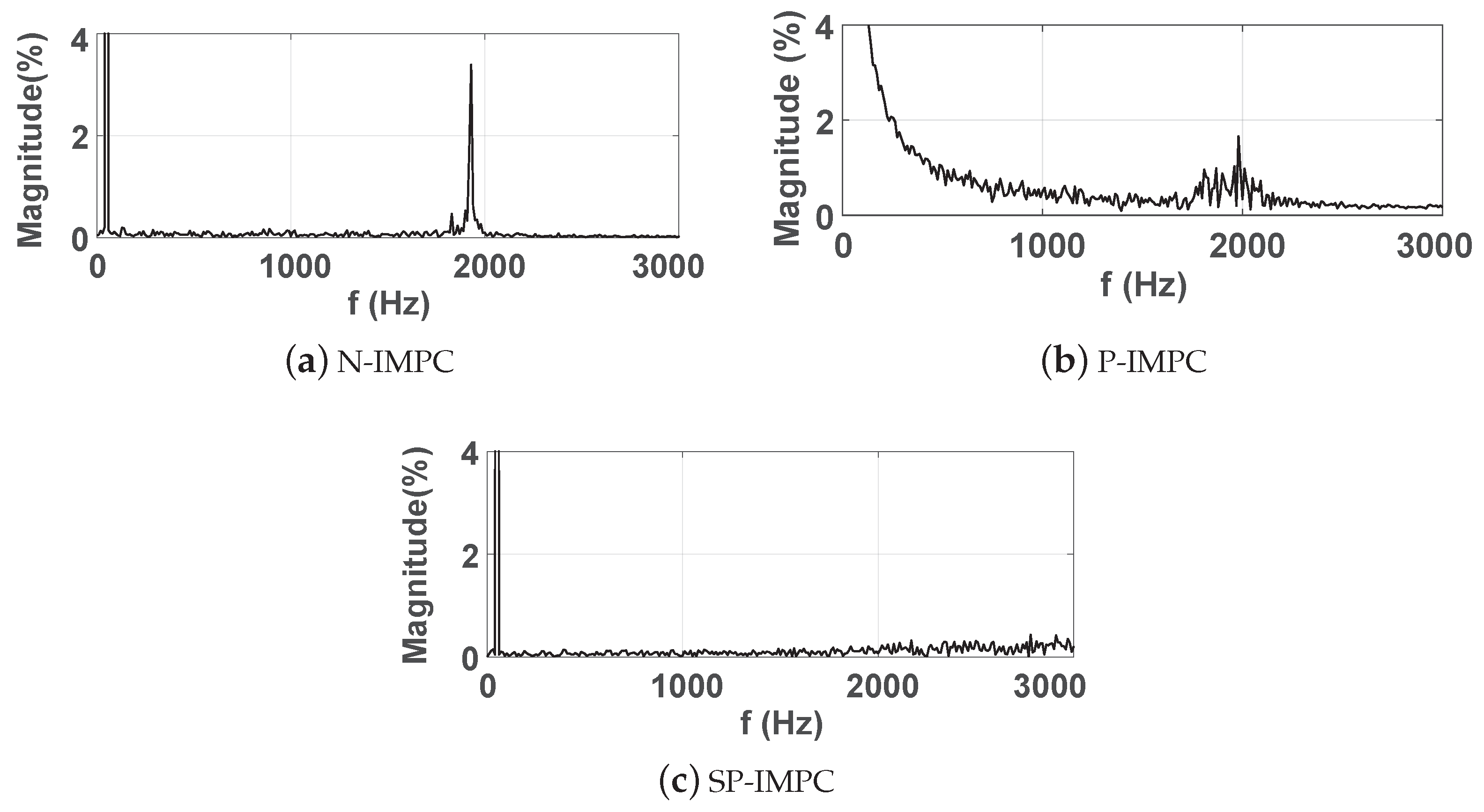
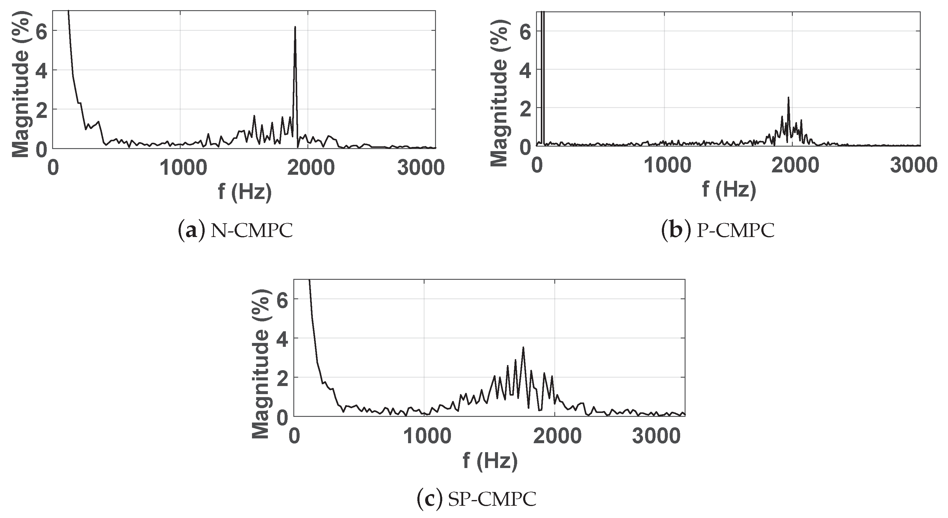
A series of tests were performed on all algorithms to compare the spectrum performance of each method using the experimental setup. That can be verified in Figure 13 and Figure 14. It can be concluded from the figures that N-IMPC and N-CMPC have higher spectrum magnitude than the P-CMPC and P-IMPC. It can be seen also that it is difficult to keep the spectrum magnitude at the desired frequency in case of using SP-IMPC. Bearing in mind that the SP-CMPC can not be operating at exactly 2 kHz. All these findings make P-IMPC the best algorithm, among the discussed ones in this paper, in terms of fixed switching frequency while providing high power quality. In addition, it is easy to obtain the reference switching frequency and follow it accurately.

Table 2. Relative Importance between Objectives

Relative Importanace	Frequency Control Methods	Improved MPC (IMPC)
Case I	High importance	Low importance
Case II	Equal importance	Equal importance
Case III	Low importance	High importance

summarizes the THDv for each method utilizing the same LC filter design. It can be concluded that periodic control has a better THDv in both the conventional and improved FCS-MPC.

□

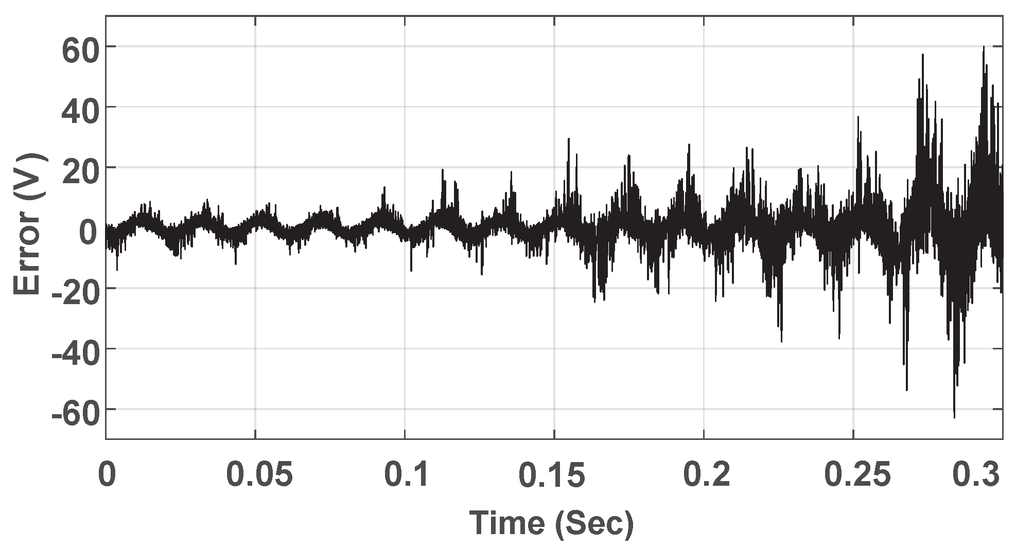
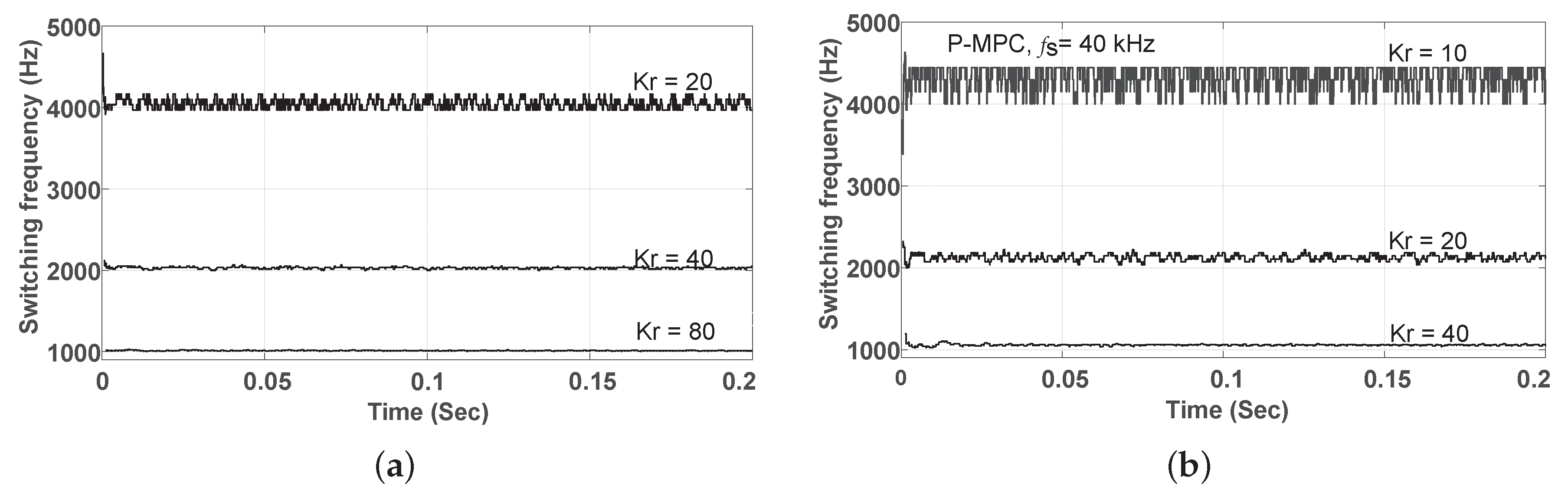
Figure 15 shows the measured switching frequency in cases where using the P-CMPC and P-IMPC as discussed in Equation (29). It depicts that in P-IMPC, the deviation from the reference is a little higher compared to the conventional P-CMPC, and the reason is that the weighting factors for both tests, in this case, were kept constant. That was to illustrate the effect of using the same weighting factors for both algorithms.

□

Figure 16a,b show two important aspects. Firstly, they show how the periodic control strategy follows the different references resulting in a fixed switching frequency. Secondly, they show the effect of samplings, which indicates that P-CMPC and P-IMPC are using high sampling frequency to give better fixed switching frequency performance.

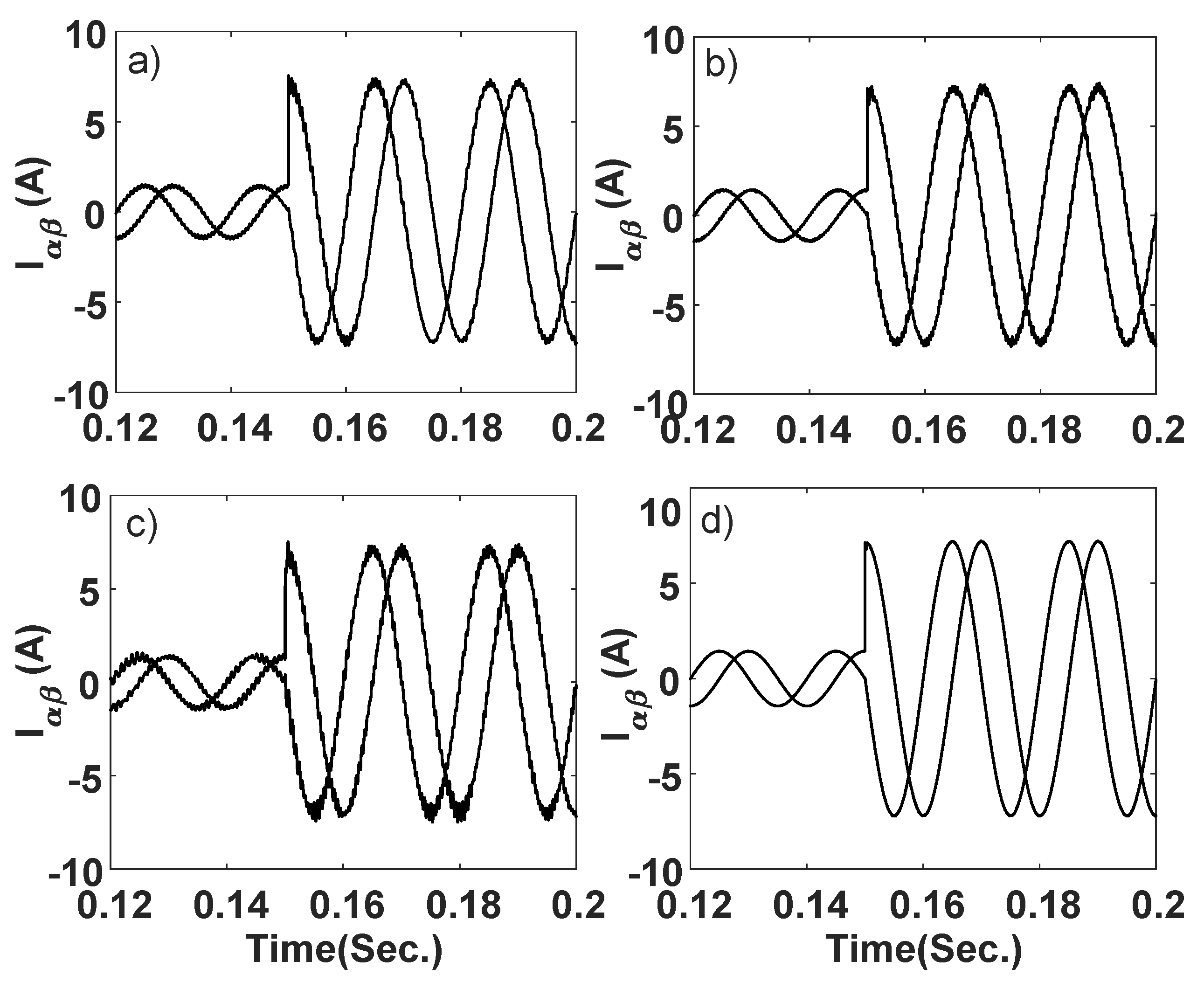
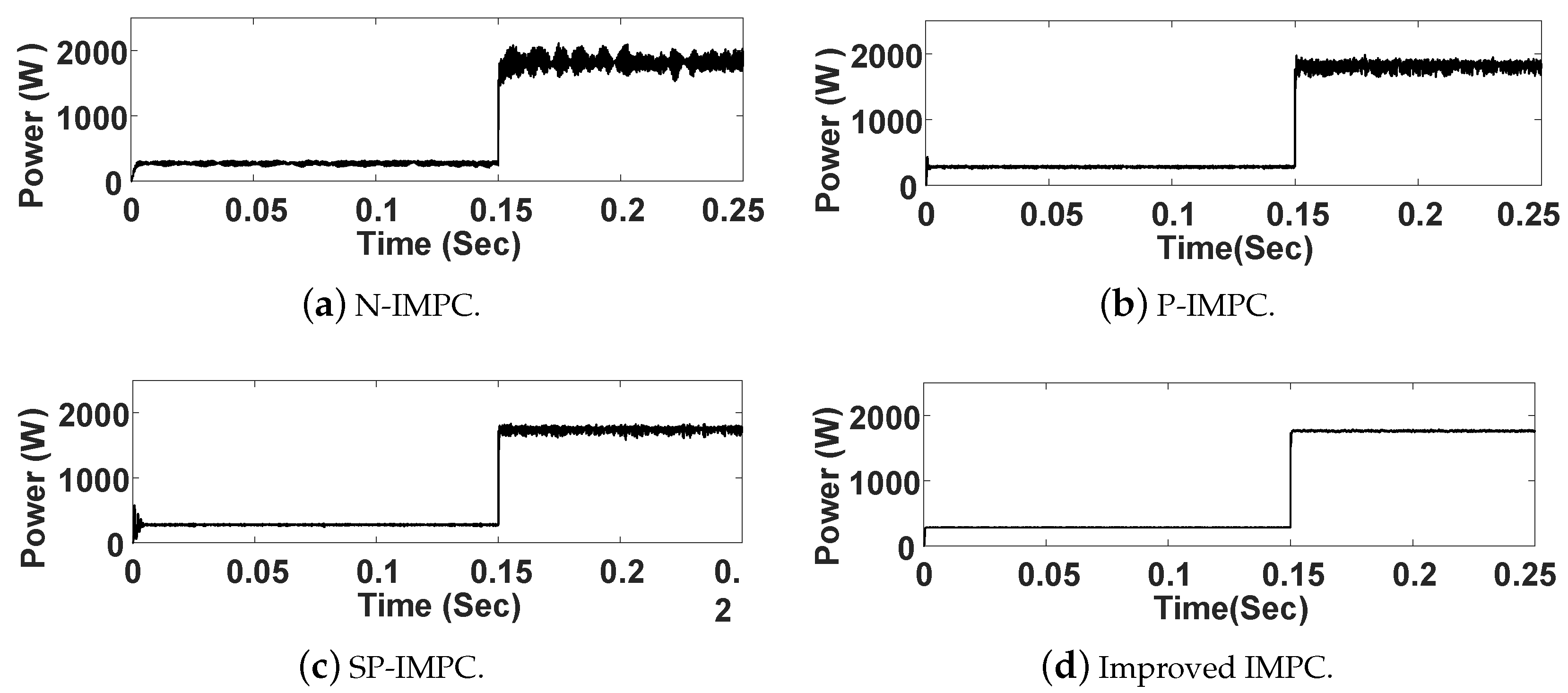
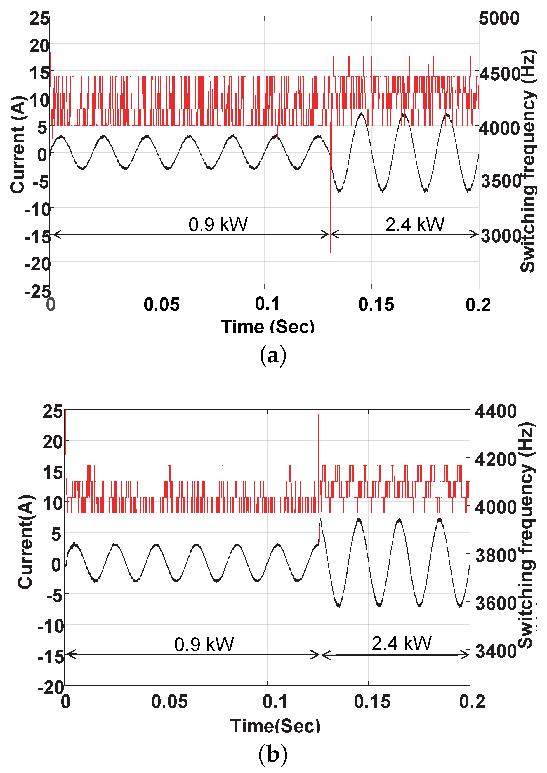
4.2. Dynamic Response

All FCS-MPC algorithms were discussed in this work have been tested in order to observe the dynamic operation in case of load changes. A power change of more than 30% of the total power has occurred suddenly in order to test all controllers. As shown in Figure 17, it can be seen that $\alpha \beta$ currents using SP-IMPC, N-IMPC, and P-IMPC still responded to the instant load changes exactly the same as the IMPC. One reason behind this is the accurate design of each CF, which guarantees no conflicts between the several objectives in one CF. Furthermore, Figure 18 and Figure 19 show the power deviation of conventional and improved CFs with/without including the frequency control terms. Due to the ability of the IMPC to better regulate the voltage and current quantities, the power deviation in case of using frequency control terms with IMPC shows promising results.

Finally, it has to be noticed that a proper low-pass filter and correct weight factors design are crucial to preserve the dynamic properties of the proposed algorithms and obtain the best possible power quality.

4.3. Sampling Effect

As the sampling time ($T_s$) decreases, the rejection of disturbances usually improves. However, when ($T_s$) becomes too small, the computational effort increases dramatically. Therefore, the optimal choice is a balance of computational burden and power quality. Figure 20a,b show two points; initially, they confirm that the frequency control algorithms are significantly influenced by sampling time values. Secondly, they show how samplings affect the dynamic changes when a load step is applied. The presented results show the behaviour of the predictive control implemented using periodic control for the grid forming application. It can be seen that the deviation in the case of 40 kHz sampling is high and varies between 4 kHz and 4.5 kHz, while in the 80 kHz the variance is between 4 kHz and 4.15 kHz.

4.4. Steady-State Operation

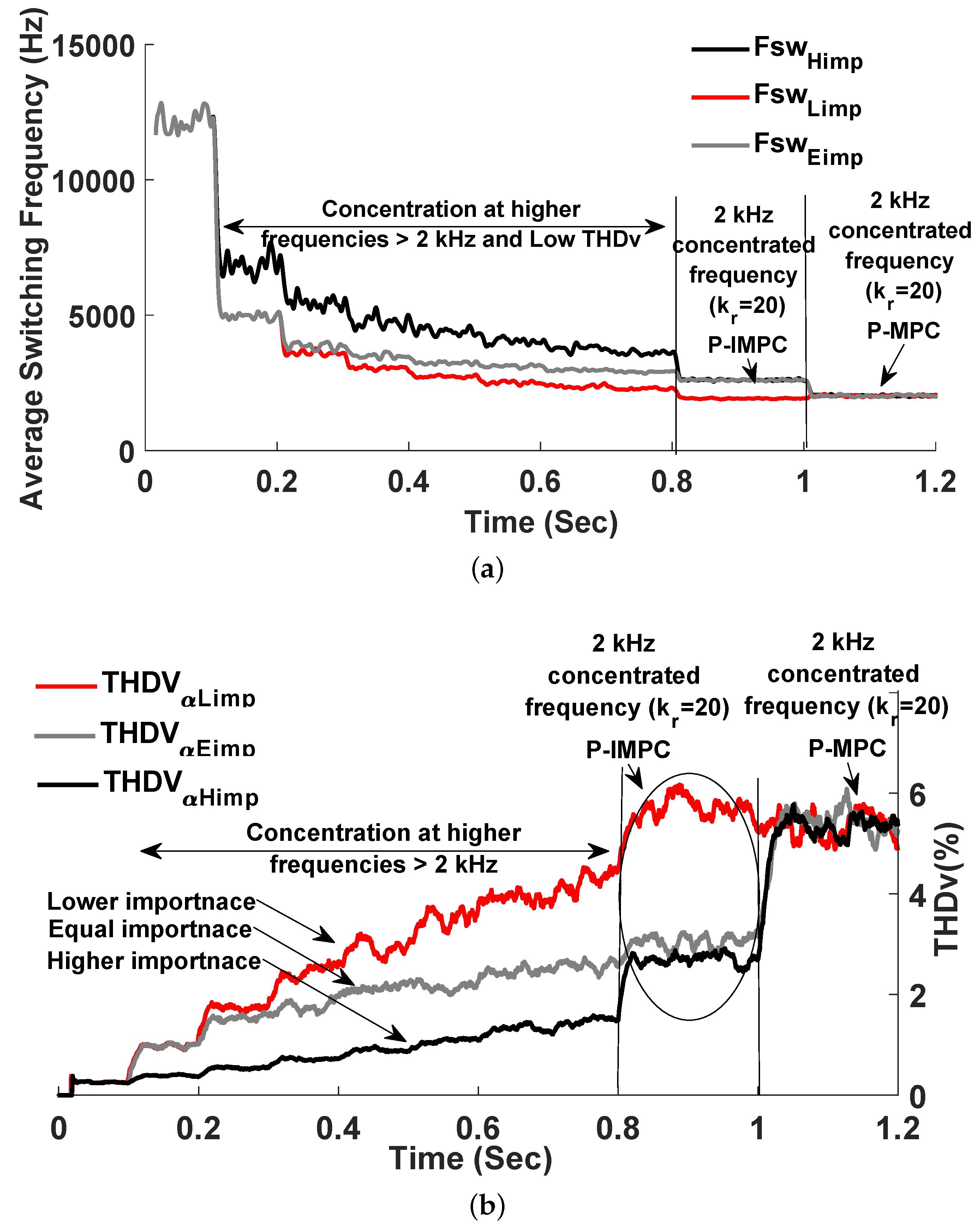
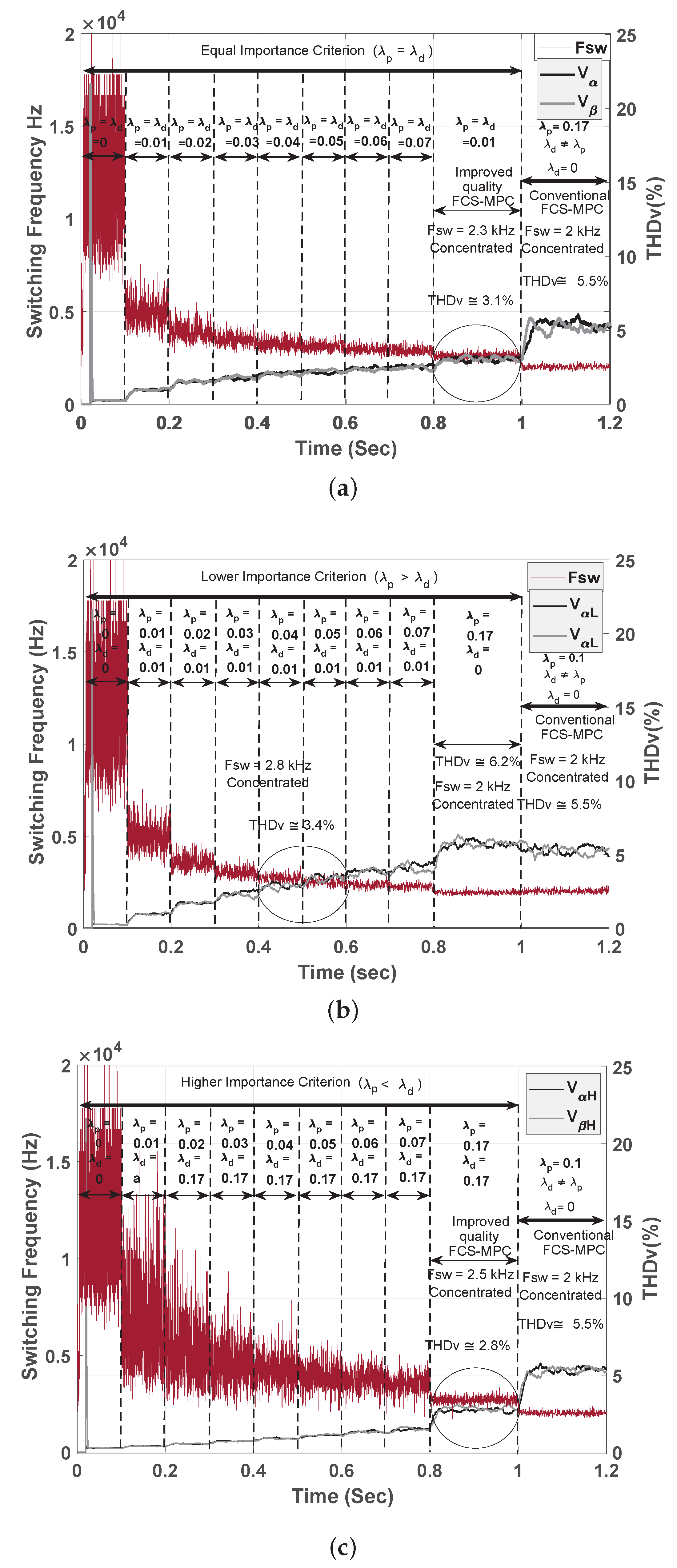
For the steady-state performance evaluation, all FCS-MPC algorithms were discussed in this work have been observed during the steady-state operation. Apparently and during the tests stage, all algorithms showed very good performance in terms of controller stability. However, N-CMPC requires more computation time, which introduces some difficulties in the implementation. On the other hand, the power qualites of N-IMPC, SP-IMPC, and P-IMPC have a significant improvement compared to N-CMPC, SP-CMPC, and P-CMPC. The P-IMPC has around 5% reduction in the active power fluctuation comparing to the P-CMPC, which is a significant outcome compared to the N-IMPC and SP-IMPC. Bearing in mind that the steady-state performance of all algorithms can be observed also in Figure 11, Figure 12, Figure 17 and Figure 20.

4.5. Factor weights

Three optimization criteria have been employed in this paper in order to choose the best factor values and maintain system stability. Mainly, the tuning process was based on the relative importance between the objectives and in this work, the tuning processes of P-CMPC and P-IMPC schemes are shown as an example. Normally, there are no specific guidelines to determine the exact tuning factors of any multi-objective function. In this paper, the relative importance between objectives was determined by defining the priority of each objective. As shown in Figure 21, different tuning of P-IMPC gives somehow a reduced switching frequency until the fixed switching behaviour is reached at 0.8 s and at 1 s for P-CMPC. The importance which is given to the periodic objective determines how the output performance is, in terms of the fixed switching frequency. It worth to mention that power quality is greatly maintained. Figure 22 demonstrates the performance of P-CMPC and P-IMPC during the selection of weighting factors for all three cases, which are defined in Table 2. It can be seen that both equal and higher importance criterion give very good results in terms of switching frequency and THDv for P-IMPC. In the end,

Table 3. Characteristics of the implemented conventional and proposed MPC schemes.

	CMPC without Frequency Control	IMPC without Frequency Control	CMPC + SP-Control	IMPC + SP-Control	CMPC + Notch Control	IMPC + Notch Control	CMPC + Periodic Control	IMPC + Periodic Control
THDv	Low	Low	High	Low	High	Low	High	Low
Stability	Stable	Stable	Stable	Stable	Stable at high frequencies	Stable	Stable	Stable
Switching frequency	Variable	Variable	Reduced- variable	Reduced- variable	Variable	Variable	Fixed	Fixed
Implementation	Intuitive very easy	Intuitive very easy	Intuitive very easy	Intuitive very easy	Intuitive easy	Intuitive easy	Intuitive easy	Intuitive easy
Computational burden	1.056225 s	1.0583 s	1.0672 s	1.0694 s	1.1788 s	1.1812 s	1.0775 s	1.0859 s
Weighting factors	No Factors	${\lambda }_d$	${\lambda }_{sw}$	${\lambda }_d,{\lambda }_{sw}$	${\lambda }_n$	${\lambda }_d$, ${\lambda }_n$	${\lambda }_p$	${\lambda }_d$, ${\lambda }_p$
Transient	Excellent 0.0035 s	Excellent 0.0030 s	Excellent 0.042 s	Excellent 0.037 s	Excellent 0.059 s	Excellent 0.052 s	Excellent 0.040 s	Excellent 0.035 s
Output THDv	0.7%	0.3%	$7.52\%$	$2.62\%$	$5.67\%$	$4.14\%$	$5.51\%$	$3.11\%$
Current error	$0.159\%$	$0.07\%$	$3.90\%$	$1.35\%$	$2.23\%$	$1.51\%$	$2.62\%$	$0.23\%$
Sampling time (Ts)	40 kHz	40 kHz	40 kHz	40 kHz	40 kHz	40 kHz	40 kHz	40 kHz
Switching frequency	Avg ≈ 12 kHz	Avg ≈ 11.5 kHz	Desired frequency + large error ≈ 2 kHz	Desired frequency + large error ≈ 2 kHz	Desired frequency + large error ≈ 2 kHz	Desired frequency + large error ≈ 2 kHz	Desired frequency + small error ≈ 2 kHz	Desired frequency + small error ≈ 2 kHz
Output filter size	L = 5 mH C = 60 μF can be optimized to L = 2.3 mH, C = 25 μF	L = 5 mH C = 60 μF can be optimized to L = 2.3 mH, C = 15 μF	L = 5 mH C = 60 μF	L = 5 mH C = 60 μF	L = 5 mH C = 60 μF	L = 5 mH C = 60 μF	L = 3 mH C = 60 μF can be optimized to L = 3 mH, C = 40 μF	L = 5 mH C = 60 μF can be optimized to L = 3 mH, C = 40 μF

summarizes the characteristics of all eight algorithms to have an overview of their features. The Table includes THDv, stability assessment, implementation, computational burden, and switching behaviour.

5. Conclusions

In this work, a proposal of an improved FCS-MPC is presented, and the suitability of three different frequency control approaches has been investigated. The frequency control algorithms with the improved scheme introduced new FCS-MPC regulators for grid forming converters. The primary objective of the CF is to predict the voltage, while the secondary objective is to improve the power quality for enhancement purposes. In order to have similar characteristics as the conventional linear controllers, FCS-MPC should control the switching frequency and reshape the spectrum at desired values. One advantage is to reduce the losses by reducing the average switching frequency, where the new CFs do not introduce a high computational burden. Another advantage is to control system, which uses only one-step prediction. In this respect, the steady-state performance of the system becomes comparable with some recent proposed FCS-MPCs, which achieve good power quality using longer horizon or multi-step prediction. Besides, this work has shown that the frequency can be concentrated, while the feature of the fast dynamic response is retained. Some challenges have been solved during this work-study, and there were as follows:

□

Weight factors tuning, which affects the performance of the power converter. This challenge solved by defining the importance of each objective in multi-objective CF.

□

Another challenge was to include the most suitable frequency control objectives without using a modulator and send the optimized actuation based on the error evaluated by the CF. This challenge has been solved by investigating the performance of each frequency control scheme combined with the improved FCS-MPC.

□

High-frequency sampling, which is solved by concentrating the switching frequency at a relatively lower frequency. That allowed the standard setups to handling this kind of controllers.

In the end, this work showed that the proposed derivative, FCS-MPC based scheme could improve any approach introduced so far for controlling the switching frequency. Periodic control achieved promising results in terms of power quality and fixed switching behaviour. Moreover, periodic control has a simple and easy implementation for further consideration in the grid-forming applications. The proposed cost function is applicable for complicated systems such as the matrix or neutral point clamped converters. The idea behind using VSC is to simply illustrate the new schemes and verify the frequency control methods and providing some comparisons. As future work, researchers are seeking new techniques to eliminate the weighting factors or using intelligent technologies in order to calculate the weighting factors online resulting in much more flexibility.

References

1. Rahman, M.S.; Hossain, M.J.; Lu, J.; Pota, H.R. A Need-Based Distributed Coordination Strategy for EV Storages in a Commercial Hybrid AC/DC Microgrid With an Improved Interlinking Converter Control Topology. IEEE Trans. Energy Convers. 2018, 33, 1372–1383. [Google Scholar] [CrossRef] [Green Version]
2. Khalili, T.; Hagh, M.T.; Zadeh, S.G.; Maleki, S. Optimal reliable and resilient construction of dynamic self-adequate multi-microgrids under large-scale events. IET Renew. Power Gener. 2019, 13, 1750–1760. [Google Scholar] [CrossRef]
3. Peyghami, S.; Mokhtari, H.; Davari, P.; Loh, P.C.; Blaabjerg, F. On Secondary Control Approaches for Voltage Regulation in DC Microgrids. IEEE Trans. Ind. Appl. 2017, 53, 4855–4862. [Google Scholar] [CrossRef] [Green Version]
4. Peyghami, S.; Mokhtari, H.; Loh, P.C.; Davari, P.; Blaabjerg, F. Distributed Primary and Secondary Power Sharing in a Droop-Controlled LVDC Microgrid With Merged AC and DC Characteristics. IEEE Trans. Smart Grid 2018, 9, 1949–3053. [Google Scholar] [CrossRef] [Green Version]
5. Wang, S.; Liu, Z.; Liu, J.; Liu, B.; Meng, X.; An, R. Modeling and analysis of droop based hybrid control strategy for parallel inverters in islanded microgrids. In Proceedings of the 2017 IEEE Applied Power Electronics Conference and Exposition (APEC), Tampa, FL, USA, 26–30 March 2017; pp. 3462–3469. [Google Scholar] [CrossRef]
6. Chen, Z.; Pei, X.; Yang, M.; Peng, L. An Adaptive Virtual Resistor (AVR) Control Strategy for Low-Voltage Parallel Inverters. IEEE Trans. Power Electron. 2018, 34, 863–876. [Google Scholar] [CrossRef]
7. Hou, X.; Sun, Y.; Lu, J.; Zhang, X.; Koh, L.H.; Su, M.; Guerrero, J.M. Distributed Hierarchical Control of AC Microgrid Operating in Grid-Connected, Islanded and Their Transition Modes. IEEE Access 2018, 6, 77388–77401. [Google Scholar] [CrossRef]
8. Wang, J.; Jin, C.; Wang, P. A Uniform Control Strategy for the Interlinking Converter in Hierarchical Controlled Hybrid AC/DC Microgrids. IEEE Trans. Ind. Electron. 2017, 65, 6188–6197. [Google Scholar] [CrossRef]
9. Davari, P.; Yang, Y.; Zare, F.; Blaabjerg, F. Predictive Pulse-Pattern Current Modulation Scheme for Harmonic Reduction in Three-Phase Multidrive Systems. IEEE Trans. Ind. Electron. 2016, 63, 5932–5942. [Google Scholar] [CrossRef] [Green Version]
10. La Bella, A.; Cominesi, S.R.; Sandroni, C.; Scattolini, R. Hierarchical Predictive Control of Microgrids in Islanded Operation. IEEE Trans. Autom. Sci. Eng. 2016, 14, 536–546. [Google Scholar] [CrossRef]
11. Vazquez, S.; Leon, J.I.; Franquelo, L.G.; Rodriguez, J.; Young, H.A.; Marquez, A.; Zanchetta, P. Model Predictive Control: A Review of Its Applications in Power Electronics. IEEE Ind. Electron. Mag. 2014, 8, 16–31. [Google Scholar] [CrossRef]
12. Young, H.; Rodríguez, J. Comparison of finite-control-set model predictive control versus a SVM-based linear controller. In Proceedings of the 2013 15th European Conference on Power Electronics and Applications (EPE), Lille, France, 2–6 September 2013; pp. 1–8. [Google Scholar] [CrossRef]
13. Jiang, C.; Du, G.; Du, F.; Lei, Y. A Fast Model Predictive Control with Fixed Switching Frequency Based on Virtual Space Vector for Three-Phase Inverters. In Proceedings of the IEEE International Power Electronics and Application Conference and Exposition, Shenzhen, China, 4–7 November 2018; pp. 1–7. [Google Scholar] [CrossRef]
14. He, J.; Li, Y.W. Generalized Closed-Loop Control Schemes with Embedded Virtual Impedances for Voltage Source Converters with LC or LCL Filters. IEEE Trans. Power Electron. 2012, 27, 1850–1861. [Google Scholar] [CrossRef]
15. Escobar, G.; Mattavelli, P.; Stankovic, A.M.; Valdez, A.A.; Leyva-Ramos, J. An Adaptive Control for UPS to Compensate Unbalance and Harmonic Distortion Using a Combined Capacitor/Load Current Sensing. IEEE Trans. Ind. Electron. 2007, 54, 839–847. [Google Scholar] [CrossRef]
16. Khan, H.S.; Aamir, M.; Ali, M.; Waqar, A.; Ali, S.U.; Imtiaz, J. Finite Control Set Model Predictive Control for Parallel Connected Online UPS System under Unbalanced and Nonlinear Loads. Energies 2019, 12, 581. [Google Scholar] [CrossRef] [Green Version]
17. Rodriguez, J.; Pontt, J.; Silva, C.A.; Correa, P.; Lezana, P.; Cortés, P.; Ammann, U. Predictive Current Control of a Voltage Source Inverter. IEEE Trans. Ind. Electron. 2007, 54, 495–503. [Google Scholar] [CrossRef]
18. Cortés, P.; Ortiz, G.; Yuz, J.I.; Rodríguez, J.; Vazquez, S.; Franquelo, L.G. Model Predictive Control of an Inverter With Output LC Filter for UPS Applications. IEEE Trans. Ind. Electron. 2009, 56, 1875–1883. [Google Scholar] [CrossRef]
19. Cortes, P.; Rodriguez, J.; Vazquez, S.; Franquelo, L.G. Predictive control of a three-phase UPS inverter using two steps prediction horizon. In Proceedings of the IEEE International Conference on Industrial Technology, Vina del Mar, Chile, 14–17 March 2010; pp. 1283–1288. [Google Scholar] [CrossRef] [Green Version]
20. Hosseinzadeh, M.A.; Sarbanzadeh, M.; Sarebanzadeh, E.; Rivera, M.; Munoz, J. Predictive Control in Power Converter Applications: Challenge and Trends. In Proceedings of the IEEE International Conference on Automation/XXIII Congress of the Chilean Association of Automatic Control, Concepcion, Chile, 17–19 October 2018; pp. 1–6. [Google Scholar] [CrossRef]
21. Hosseinzadeh, M.A.; Sarbanzadeh, M.; Sarbanzadeh, E.; Rivera, M.; Gregor, R. Recent Challenge and Trends of Predictive Control in Power Electronics Application. In Proceedings of the International Conference on Electrical Systems for Aircraft, Railway, Ship Propulsion and Road Vehicles International Transportation Electrification Conference, Nottingham, UK, 7–9 November 2018; pp. 1–6. [Google Scholar] [CrossRef]
22. Alhasheem, M.; Dragicevic, T.; Blaabjerg, F.; Davari, P. Parallel Operation of Dual VSCs Regulated by FCS-MPC Using Droop Control Approach. In Proceedings of the 20th European Conference on Power Electronics and Applications, Riga, Latvia, 17–21 September 2018; pp. 1–10. [Google Scholar]
23. Peyghami, S.; Alhasheem, M.A.M.Z.Y.; Blaabjerg, F. Power Electronics-Microgrid Interfacing. In Variability, Scalability and Stability of Microgrid; Institution of Engineering and Technology: London, UK, 2019. [Google Scholar] [CrossRef]
24. Vazquez, S.; Leon, J.I.; Franquelo, L.G.; Carrasco, J.M.; Martinez, O.; Rodriguez, J.; Cortes, P.; Kouro, S. Model Predictive Control with constant switching frequency using a Discrete Space Vector Modulation with virtual state vectors. In Proceedings of the IEEE International Conference on Industrial Technology, Gippsland, VIC, Australia, 10–13 February 2009; pp. 1–6. [Google Scholar] [CrossRef] [Green Version]
25. Alhasheem, M.; Dragicevic, T.; Blaabjerg, F. Evaluation of multi predictive controllers for a two-level three-phase stand-alone voltage source converter. In Proceedings of the IEEE Southern Power Electronics Conference, Puerto Varas, Chile, 4–7 December 2017; pp. 1–6. [Google Scholar] [CrossRef]
26. Geyer, T.; Quevedo, D.E. Performance of Multistep Finite Control Set Model Predictive Control for Power Electronics. IEEE Trans. Power Electron. 2015, 30, 1633–1644. [Google Scholar] [CrossRef]
27. Zhang, Y.; Liu, J.; Fan, S. On the inherent relationship between finite control set model predictive control and SVM-based deadbeat control for power converters. In Proceedings of the IEEE Energy Conversion Congress and Exposition, Cincinnati, OH, USA, 1–5 October 2017; pp. 4628–4633. [Google Scholar] [CrossRef]
28. Alhasheem, M.; Dragicevic, T.; Rivera, M.; Blaabjerg, F. Losses evaluation for a two-level three-phase stand-alone voltage source converter using model predictive control. In Proceedings of the IEEE Southern Power Electronics Conference, Puerto Varas, Chile, 4–7 December 2017; pp. 1–6. [Google Scholar] [CrossRef]
29. Tomlinson, M.; du Toit Mouton, H.; Kennel, R.; Stolze, P. A Fixed Switching Frequency Scheme for Finite-Control-Set Model Predictive Control—Concept and Algorithm. IEEE Trans. Ind. Electron. 2016, 63, 7662–7670. [Google Scholar] [CrossRef]
30. Rivera, M. Predictive current control for a VSI with reduced common mode voltage operating at fixed switching frequency. In Proceedings of the IEEE 24th International Symposium on Industrial Electronics, Buzios, Brazil, 3–5 June 2015; pp. 980–985. [Google Scholar] [CrossRef]
31. Rodriguez, J.; Cortes, P. Predictive Control of Power Converters and Electrical Drives; John Wiley & Sons: Hoboken, NJ, USA, 2012; Volume 40. [Google Scholar] [CrossRef]
32. Aguirre, M.; Kouro, S.; Rojas, C.A.; Rodriguez, J.; Leon, J.I. Switching Frequency Regulation for FCS-MPC Based on a Period Control Approach. IEEE Trans. Ind. Electron. 2018, 65, 5764–5773. [Google Scholar] [CrossRef]
33. Cortes, P.; Rodriguez, J.; Silva, C.; Flores, A. Delay Compensation in Model Predictive Current Control of a Three-Phase Inverter. IEEE Trans. Ind. Electron. 2012, 59, 1323. [Google Scholar] [CrossRef]
Figure 1. (a) Schematic representation of an islanded microgrid; and (b) the electrical model of the VSC.
Applsci 10 06390 g001
Figure 2. Power circuit and FCS-MPC control structure of a standalone inverter for microgrid applications.
Applsci 10 06390 g002
Figure 3. Voltage vectors generated by the inverter ( V i ) .
Applsci 10 06390 g003
Figure 4. Simulation result for the (SP-CMPC): Switching frequency reduction during sweeping the weighting factor λ s w using the CF in Equation (21) with the conventional tracking system.
Applsci 10 06390 g004
Figure 5. Simulation result for the (SP-CMPC): instantaneous voltage error during sweeping the weighting factor λ s w in the same manner as the above figure using the CF in Equation (21) with the conventional tracking system.
Applsci 10 06390 g005
Figure 6. Flowchart of the implemented algorithms using dSpace.
Applsci 10 06390 g006
Figure 7. Experimental setup.
Applsci 10 06390 g007
Figure 8. A bode plot shows the frequency response of the LC, which is used in the experimental setup.
Applsci 10 06390 g008
Figure 9. Different frequency concentrations using periodic control with conventional CMPC. (a) P-CMPC at 1 kHz; (b) P-CMPC at 2 kHz; and (c) P-CMPC at 4 kHz.
Applsci 10 06390 g009
Figure 10. The spectrum of the conventional CF (CMPC).
Applsci 10 06390 g010
Figure 11. Experimental results of output load current (phase a) with its corresponding spectrum utilizing periodic control (P-CMPC).
Applsci 10 06390 g011
Figure 12. Obtained experimental voltage and spectrum results using the conventional and improved CFs. F s w = 2 kHz, C f = 60 μF, L f = 5 mH.
Applsci 10 06390 g012
Figure 13. Obtained experimental spectrum results using three different frequency control methodologies with improved CF (IMPC). (a) Notch control; (b) periodic control; and (c) simple penalization control.
Applsci 10 06390 g013
Figure 14. Obtained experimental spectrum results using three different frequency control methodologies with conventional CF (CMPC). (a) Notch control; (b) periodic control; and (c) simple penalization control.
Applsci 10 06390 g014
Figure 15. The measured switching frequency for the conventional and improved CFs using a periodic control strategy.
Applsci 10 06390 g015
Figure 16. The effectiveness of periodic control at different reference frequencies using two sampling values. (a) 80 kHz sampling; and (b) 40 kHz sampling. (a) The switching frequency measurements for different references K r ; (b) The switching frequency measurements for different references K r .
Applsci 10 06390 g016
Figure 17. Obtained experimental results for the dynamic response of the VSC using the proposed CFs, load step from 270 W to 1900 W, where (a) is the dynamic response for (N-IMPC) strategy, (b) periodic (P-IMPC), (c) simple penalization (SP-IMPC), and (d) without frequency control (IMPC).
Applsci 10 06390 g017
Figure 18. Dynamic response of active power using frequency control methodologies with the conventional CF (CMPC). (a) Notch filter control using the conventional CF (N-CMPC); (b) periodic control using the conventional CF (P-CMPC); (c) simple penalization control using the conventional CF (SP-CMPC); and (d) conventional CF (CMPC).
Applsci 10 06390 g018
Figure 19. Dynamic response of active power using frequency control methodologies with improved CF (IMPC). (a) Notch filter control using the improved CF (N-IMPC), where the power deviation is less than the conventional CF (N-CMPC) with 1.47% average; (b) periodic control using the improved CF (P-IMPC), where the power deviation is less than the conventional (P-CMPC) with 5.36% average; (c) simple penalization control using the improved CF (SP-IMPC), where the power deviation is less than the conventional CF (SP-CMPC) with 1.39% average; and (d) improved (IMPC).
Applsci 10 06390 g019
Figure 20. Sampling effect: a comparison between the switching frequency and currents response of the 40 kHz and 80 kHz samplings. (a) A step response from 2.2 kW to 5.2 kW when Ts = 25 μs; and (b) a step response from 2.2 kW to 5.2 kW when Ts = 12.5 μs. (a) Experimental results: the dynamic response for a VSC using a periodic control strategy having a 40 kHz sampling; (b) Simulated dynamic response for VSC using periodic control strategy having an 80 kHz sampling frequency.
Applsci 10 06390 g020
Figure 21. Weighting factors drifting based on the relative importance: average switching frequency and THDv of the V α for the three criteria; (black line) the derivative term is higher importance than the periodic term; (red line) the derivative term is lower importance than the periodic term; and (grey line) the derivative term is equal importance to the periodic term. (a) Average switching frequency for the three criteria; and (b) THDv of V α for the three criteria.
Applsci 10 06390 g021
Figure 22. Measured switching frequencies and THDv for the three criteria at 1 kW (a) the drift of the weights, where the derivative weighting factor λ d is equal to the periodic weighting factor λ p ; (b) the drift of the weights, where the derivative weighting factor λ d is lower than the periodic weighting factor λ p ; and (c) the drift of the weights, where the derivative weighting factor λ d is higher than the periodic weighting factor λ p . (a) Equal importance case; (b) Lower importance case; (c) Higher importance case.
Applsci 10 06390 g022