Real-Time and Robust Hydraulic System Fault Detection via Edge Computing

Abstract

We consider fault detection in a hydraulic system that maintains multivariate time-series sensor data. Such a real-world industrial environment could suffer from noisy data resulting from inaccuracies in hardware sensing or external interference. Thus, we propose a real-time and robust fault detection method for hydraulic systems that leverages cooperation between cloud and edge servers. The cloud server employs a new approach that includes a genetic algorithm (GA)-based feature selection that identifies feature-to-label correlations and feature-to-feature redundancies. A GA can efficiently process large search spaces, such as solving a combinatorial optimization problem to identify the optimal feature subset. By using fewer important features that require transmission and processing, this approach reduces detection time and improves model performance. We propose a long short-term memory autoencoder for a robust fault detection model that leverages temporal information on time-series sensor data and effectively handles noisy data. This detection model is then deployed at edge servers that provide computing resources near the data source to reduce latency. Our experimental results suggest that this method outperforms prior approaches by demonstrating lower detection times, higher accuracy, and increased robustness to noisy data. While we have a 63% reduction of features, our model obtains a high accuracy of approximately 98% and is robust to noisy data with a signal-to-noise ratio near 0 dB. Our method also performs at an average detection time of only 9.42 ms with a reduced average packet size of 179.98 KB from the maximum of 343.78 KB.

1. Introduction

Hydraulic systems are utilized in several industrial applications, including manufacturing, automobiles, and heavy machinery [1,2,3,4,5]. Monitoring the condition of hydraulic equipment is essential, as it can maintain high productivity and reduce the costs of system processes [6]. Three challenges to the formulation of fault detection in a hydraulic system exist. First, conducting automated and real-time fault detection without human intervention is difficult because of the time-sensitive requirements to maintain proper system functionality [7]. Second, industrial sensor data are now more abundant in sample quantity and dimension [8]. A hydraulic system operates with multivariate time-series data obtained from multiple sensors, so identifying errors is challenging due to complex nonlinear relationships between data. Third, real-world industrial sensors are often located within noisy environments, so the data collected from these tend to be noisy and unreliable. Noise occurs typically because of inaccuracies in sensor configurations or interference from the external environment [9]. Because operational decisions are made based on these sensor readings, the data must be more reliable. Therefore, a solution that addresses these challenges of fault detection in hydraulic systems must include establishing a real-time detection process, learning multivariate time-series sensor data, and handling noisy data.

The concept of Industry 4.0 [10] is proposed as the current state-of-the-art among IT and manufacturing that offers enhancements in product quality, real-time decision-making, and integrated systems. Advanced technologies, such as the cloud, internet of things, and artificial intelligence, are integrated into modern manufacturing [11,12]. The cloud includes the drawback of high response times due to the long-distance transmission of massive data volumes. However, real-time responses are essential for fault detection systems. Edge computing is designed to overcome this challenge by offering computational resources near the data source resulting in decreased latency and transmission costs [13]. Cooperation between cloud and edge servers must occur for real-time fault detection in hydraulic systems [14]. For example, the cloud server can utilize offline learning, such as selecting the important data to transfer and performing model training, while the real-time intelligent service of fault detection is executed on the edge server.

We propose a genetic algorithm (GA)-based feature selection method that considers feature correlations and redundancies. Sensor feature selection is incorporated to improve the fault detection model performance while simultaneously utilizing fewer data by defining which sensor data should be sent to reduce packet transmission. A GA offers an efficient solution for search without pre-training with any domain knowledge. For the fault detection model, we employ a stacked long short-term memory autoencoder (LSTM-AE) to extract features from the sequence data automatically, which performs efficiently on latent features from clean or noisy data. Finally, the pre-trained encoder is merged and re-trained with a dense layer and Softmax classifier to perform the fault detection.

The main contributions of this study include the following:

• We propose cooperation between cloud and edge servers to support a real-time fault detection system. The cloud performs feature selection and offline learning, and the edge computes online detection near the data source, which together reduces latency and transmission costs.
• We propose a GA-based feature selection that considers correlation and redundancy to ensure the selection of features that are most important and not redundant for learning.
• We propose an LSTM-AE as the fault detection model to learn the temporal relations in the time-series data and extract latent features from noisy data.

In the remainder of this paper, we explain the hydraulic system fault analysis in Section 2. Next, we review previous work dedicated to hydraulic system fault detection in Section 3. An elaboration of the proposed architecture and algorithm are presented in Section 4, Section 5, Section 6 and Section 7. We demonstrate extensive experiments to measure the effectiveness of the proposed method in Section 8. Finally, our conclusions and future research directions are discussed.

2. Hydraulic System Fault Analysis

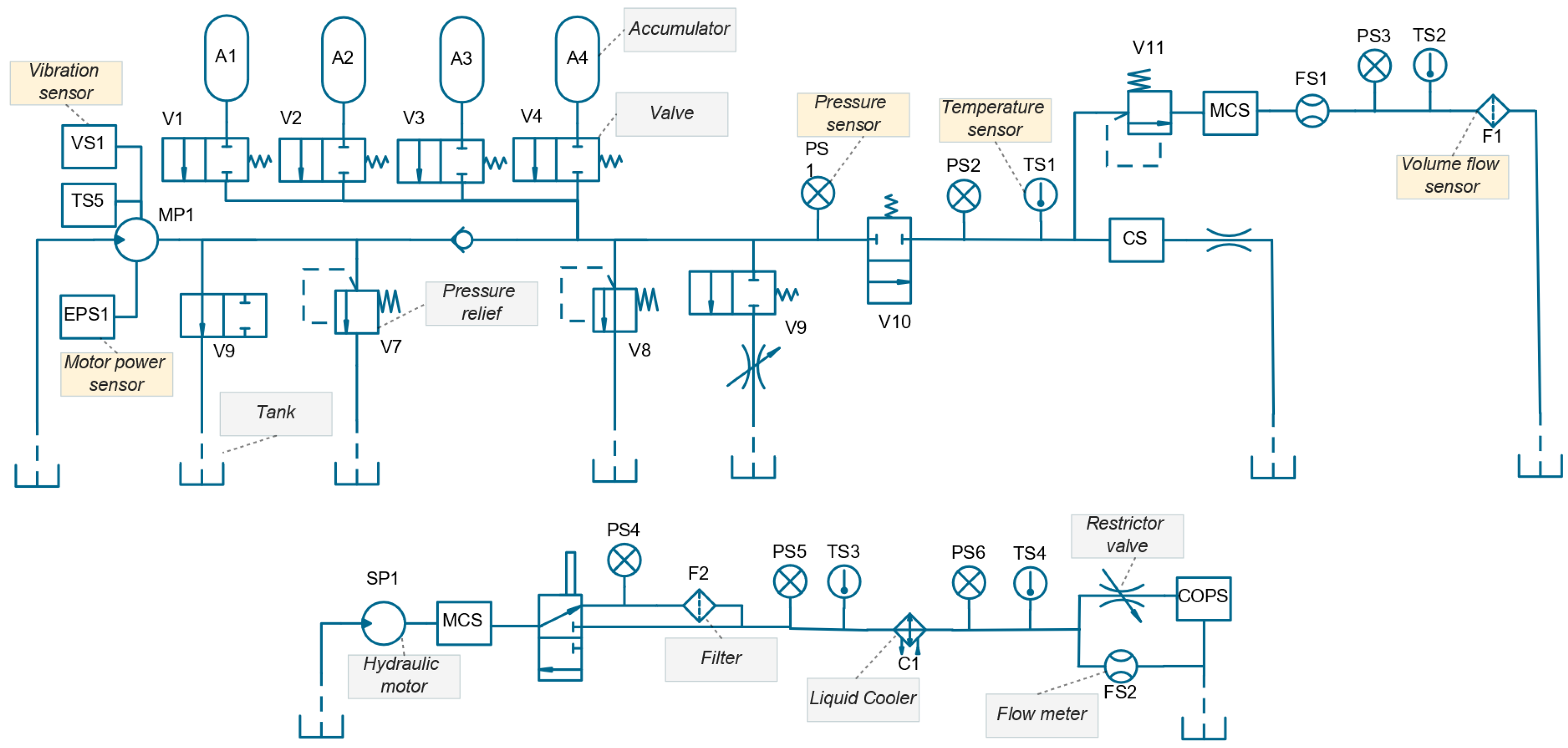
We use the hydraulic system condition monitoring dataset available from the UC Irvine Machine Learning Repository [15], which is comprised of the primary and secondary circuits shown in Figure 1. This dataset consists of 17 sensor measurements with the details of these sensor specifications listed in

Table 1. Hydraulic system sensors.

Sensor	Description	Unit	Rate (Hz)	Packet Size (KB)
PS1-6	Pressure	bar	100	47.02
EPS1	Motor power	W	100	47.02
FS1-2	Volume flow	L/min	10	4.84
TS1-4	Temperature	°C	1	0.62
VS1	Vibration	mm/s	1	0.62
CE (Virtual)	Cooling efficiency	%	1	0.62
CP (Virtual)	Cooling power	kW	1	0.62
SE (Virtual)	Efficiency factor	%	1	0.62

. The components of the hydraulic sensor include 14 physical sensors, including six pressure sensors (PS1–PS6), four temperature sensors (TS1–TS4), two volume flow sensors (FS1–FS2), a motor power sensor (EPS1), a vibration sensor (VS1), and three virtual sensors of a computed values-efficiency factor sensor (SE), a cooling efficiency sensor (CE), and a cooling power virtual sensor (CP). In addition, the hydraulic circuit maintains other sensors, such as oil parameter monitoring (COPS) and oil particle contamination (CS and MCS). Each sensor conducts measurements during a load cycle of 60 s, with sampling rates or frequencies ranging from 1 Hz to 100 Hz. The dataset consists of 2205 load cycles or samples, with each sample having a component state label corresponding to the fault condition of the components.

Table 2. Hydraulic fault component targets.

Component	Fault Condition	Control Parameter	States	Samples
Cooler (C1)	Cooling power decrease	Fan duty cycle of C1	100%: Full efficiency 20%: Reduced efficiency 3%: Close to total failure	732 732 741
Valve (V10)	Switching degradation	Switchable bypass orifices V9	100%: Optimal behavior 90%: Small lag 80%: Severe lag 73%: Close to total failure	1125 360 360 360
Pump (MP1)	Internal leakage	Control current of V10	0: No leakage 1: Weak leakage 2: Severe leakage	1221 492 492
Accumulator (A1–4)	Gas leakage	A1-4 with different pre-charge pressures	130 bar: Optimal pressure 115 bar: Slightly reduced 100 bar: Severely reduced 90 bar: Close to total failure	599 399 399 808

describes the detailed taxonomy of the fault states for the components, which includes four fault component targets of Cooler, indicating a cooling power fault, Valve, indicating a switching fault, Pump, indicating an internal pump leakage, and Accumulator, indicating a gas leak. Each type of fault includes several classes that represent various component degradation states.

3. Related Work

Edge computing is a paradigm that brings computation resources to devices on the network that are closer to the data source. Edge computing is utilized for time-sensitive applications, such as industrial condition monitoring. Park et al. [16] proposed an edge-based fault detection using an LSTM model in an industrial robot manipulator that incorporated vibration, temperature sensors, and the use of one edge device attached to the machine and pressure sensors. Syafrudin et al. [17] proposed edge-based fault detection using density-based spatial clustering and a random forest algorithm for an automobile parts factory that employed an edge model on each workstation of the assembly line. Li et al. [18] proposed edge-based visual defect detection using a convolutional neural network (CNN) model in a tile production factory that deployed multiple cameras to capture visual information of the products [19]. These data were then sent to an edge node to inspect potential defects. Even with these approaches, there remain few studies on fault detection within the context of applications in edge computing.

Several works exist that used the same data sets as in this study. Helwig et al. [15,20] convert the time domain data into frequency domain using fast fourier transform, and generate statistical features, such as the slope of the linear fit, median, variance, skewness, the position of the maximum value, and kurtosis [21]. They then calculated features for fault label correlation and selected the n features by ranking or sorting the correlation (CS). Finally, this approach applied linear discriminant analysis [22] for the fault classification. Prakash et al. [23] also utilized statistical features of frequency domain data, such as mean, skewness, and kurtosis, and applied XGBoost [24] to define feature importance (XFI) and select half of the highest correlations along with a deep neural network for the classification model. In [25], the authors proposed a dimensional reduction approach with principal component analysis (PCA) [26] to transform the raw features to a fewer number of principal component features, and then classify the faults using XGBoost. Konig et al. [27] and Yuan et al. [28] proposed a CNN [29] as the classification model into which they directly fed the raw data because CNNs can extract features.

These previous approaches include several drawbacks. First, none considered edge computing for application to hydraulic system fault detection that supports real-time detection and reduces transmission costs. Second, such statistical feature extraction, PCA, and other feature engineering methods are not suitable for real-time detection. These techniques must be applied to each new incoming sample, thereby consuming more time and computation power. Thus, directly using the raw data with less feature engineering is preferred. Third, the proposed feature selection methods, such as CS and XFI, may suffer from utilizing redundant features, as omitting redundant features would improve the model learning. Finally, noisy data in such real-world industrial environments, such as a hydraulic system, are inevitable because sensors can receive external noise factors (e.g., distorted sensor sensing) or internal factors (e.g., sensor malfunction), and no previous work addressed this issue.

With the aforementioned open issues, we propose cooperation between edge and cloud to ensure real-time detection and low transmission costs. Then, selecting and processing raw data with less extensive processing using the new approach of correlation and redundancy-aware feature selection (CRFS) that supports faster processing and better model learning. We overcome multivariate time-series and noisy data handling issues with an LSTM-AE fault detection model. Finally, the comparison between the prior works and our proposed method presented in

Table 3. Comparison with related works.

Paper	Feature Usage	Feature Selection Method	Fault Detection Model	Temporal Learning	Dimensional Reduction	Denoising
Helwig et al. [15]	Statistical feature subset	CS	LDA	✗	✓	✗
Prakash et al. [23]	Statistical feature subset	XFI	DNN	✗	✗	✗
Lei et al. [25]	Transformed features	PCA	XGBoost	✗	✓	✗
Konig et al. [27]	Transformed raw features	-	CNN	✗	✓	✗
Proposed	Raw feature subset	CRFS	LSTM-AE	✓	✓	✓

.

4. Real-Time Fault Detection in Edge Computing

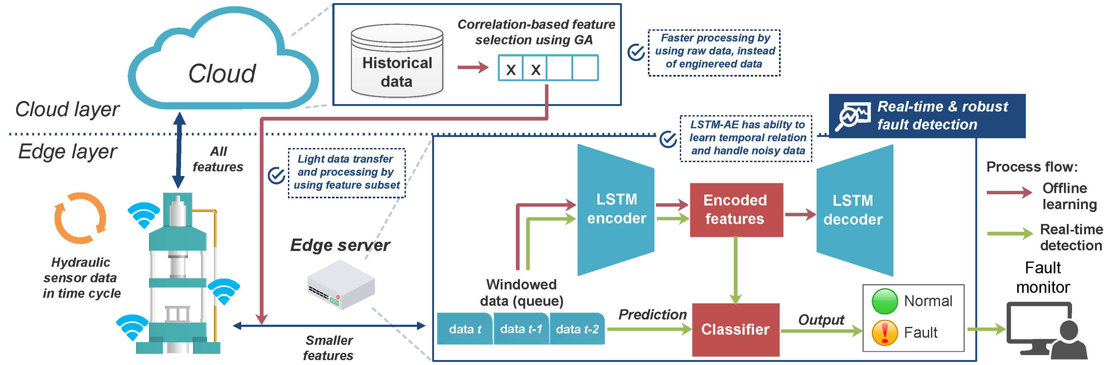
We propose a holistic framework for real-time and robust hydraulic system fault detection, as illustrated in Figure 2. The process for real-time detection is described in Algorithm 1. In lines 1–3, we conduct offline learning at the cloud server using historical data consisting of selecting the feature subsets, training the fault detection model or classifier (CLF), and deploying the model to the edge server. We use our proposed correlation and redundancy-aware feature selection to select on most relevant and less redundant features that described in detail in the Section 6. By performing the feature selection, we determine which features are essential during the fault detection process. These smaller feature subsets are directed to the edge and used for real-time detection. We pre-train an LSTM-AE, then put and tune the encoder part with a classifier layer to obtain a classifier model. These learning models will be further depicted in Section 7. By deploying the classifier model on the edge server with the features selected, the urgency of time-sensitive applications, such as fault detection, is supported. All feature data can still be sent to the cloud for collection as historical data and further analysis. Hence, the cooperation between the cloud and edge servers established in this framework provides efficient real-time fault detection for a hydraulic system.

Algorithm 1 Real-time time-series fault detection.

Input Historical data with all features f    Output Predicted output c    ▹ Offline learning at Cloud server  1: Feature selection $f_s$ based on Algorithm 2  2: Train LSTM-AE using $f_s$ based on Algorithm 3  3: Deploy trained classifier $CLF$ to Edge server    ▹ Real-time detection at Edge server  4: Initialize queue $Q=\left\{\right\}$ with size w  5: for all incoming data x with feature subset $f_s$ do  6:     Calculate mean and normalize x  7:     Push x to Q  8:     if number of elements in Q == w then  9:         Predict Q using $CLF$ model 10:         Pop top element in Q

Within a real-world scenario, the sensor data stream arrives sequentially, so these incoming data are queued, and the detection is performed on these queued elements. The window queue functions accommodate the data stream that is then fed into the LSTM model, which learns the temporal relationships between these sequence data. The incoming data include the selected features resulting from the CRFS algorithm. Therefore, our framework is suitable for general industrial systems that conduct simultaneous condition monitoring in time cycles. These processes are shown in lines 4–10.

5. Data Pre-Processing

5.1. Data Balancing

The dataset used in this study suffers from an imbalanced class distribution over several fault types, including Valve, Pump, and Accumulator components with a ratio of normal and fault class at least 1:2 or more. An imbalanced class dataset can result in our model ignoring the learning of a minority class, thereby resulting in biased model performance [30]. Thus, we perform data balancing using a random over-sampling to duplicate samples randomly from the minority class. As a result of this pre-processing, the number of component samples becomes 741 × 3 for the Cooler, 1125 × 4 for the Valve, 1221 × 3 for the Pump, and 808 × 4 for the Accumulator.

5.2. Mean and Normalization

Additional pre-processing steps are performed after the data are obtained at the edge server. First, the means of the data are calculated to obtain a single value over the different sampling rate data. Second, the incoming data are normalized in the range of 0–1. By normalizing all inputs to a standard scale, the network model can learn the optimal parameters for each input node more rapidly.

5.3. Data Windowing

Before sending the input into the fault detection model, we perform data windowing to divide and group the multivariate time-series sensor data based on the window length w, $\mathcal{X}\to \mathbf{X}$, as expressed in Equation (1). The value of w describes how many time-steps are processed, and the length of data changes from t to $n=t-w+1$ sequences, as shown in Equation (2):

$$\begin{array}{c}{\mathbf{x}}_1=[x_1,\dots ,x_w]\hfill \\ {\mathbf{x}}_2=[x_2,\dots ,x_{w+1}]\hfill \\ {\mathbf{x}}_n=[x_n,\dots ,x_t]\hfill \end{array}$$

(1)

$$\begin{array}{c}\mathcal{X}=[x_1,x_2,\dots ,x_t]\hfill \\ \mathbf{X}=[{\mathbf{x}}_1,{\mathbf{x}}_2,\dots ,{\mathbf{x}}_n]\hfill \end{array}$$

(2)

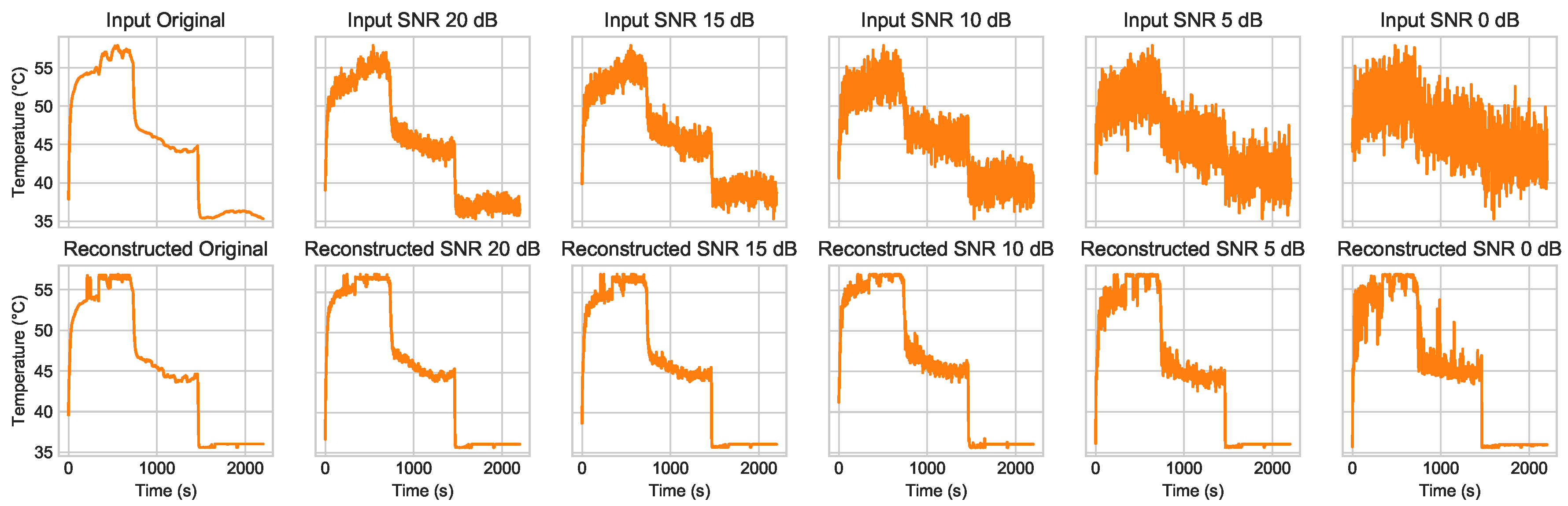
5.4. Adding Noise

We also evaluate the robustness of our proposed method against noise as compared to the prior works described earlier. We add noise at different levels to the raw sensor data, as illustrated with the temperature sensor TS1, presented in Figure 3. Each figure shows the sensor data applied with a different noise degree in the signal-to-noise ratio ($SNR$), as defined in Equation (3), where $P_{noise}$ represents the power of the noise, and $P_{signal}$ represents the power of the signal:

$$SN{R}_{dB}=10{log}_{10}\left(\frac{P_{signal}}{P_{noise}}\right)$$

(3)

6. Correlation and Redundancy-Aware Feature Selection Using a Genetic Algorithm

A GA is designed to find optimal solutions within a large search space by exploiting the process of natural selection. As a GA can discover more fit solutions after each generation, it can then identify the best solution among these [31]. Thus, a GA does not require domain knowledge to assist in the search process. Three standard operators exist to regulate the population, including a selection, crossover, and mutation operator. The selection operator determines the parents from the population, and the crossover operator defines a recombination method between the parents. Then, the mutation operator defines the genetic diversity among the offspring. The GA iterations are terminated when a pre-defined stopping criterion is met, which typically is a maximum generation number. In terms of the feature selection problem, the GA considers all possible subsets of the given feature set [32]. The individual is represented as an n-bit binary string that reflects a certain feature subset. Each bit represents the elimination or inclusion of the related feature, such that 0 represents elimination, and 1 represents the inclusion of the feature.

The CRFS process is presented in Algorithm 2 and follows the goal of selecting features based on their correlation. CRFS adopts the non-dominated sorting genetic algorithm (NSGA) that works with the multiobjective problem [33]. CRFS minimizes three objectives formulated in Equation (5). First, $g_{co{r}_o}\left(x\right)$ attempts to obtain features with a high correlation to the output label, which is important for the learning process. Second, $g_{co{r}_f}\left(x\right)$ maintains the selected features that have a low correlation to each other because high feature-to-feature correlations represent redundant features. Avoiding these redundant features results in fewer feature subsets, reduces model overfitting, and enables the model to identify interactions and important interrelated information better [34]. In our case, length n is 17 representing the number of all sensor features, and k is the number of features included in the solution. These objectives ensure that the selected features have a high correlation, low redundancy, and are part of a smaller feature subset. CRFS automatically defines the number of selected features because it is included in the objective. At the end of the iteration, we obtain the non-dominated individuals at the Pareto front, from which we select only one solution by first normalizing the values and then applying the weight (importance) of each objective with respect to the others.

In lines 2–3 of Algorithm 2, CRFS calculates the Pearson correlation coefficient [35] using Equation (4), which represents the linear relationship between two variables ranging between −1 and 1. The values of −1 and 1 represent a perfect relationship, while 0 indicates the absence of a relationship between the variables. We take the absolute value because 1 and −1 have the same meaning, and then we run the NSGA from lines 4 through 13. In line 14, we obtain the non-dominated individuals at the Pareto front and select the fittest one among these by scaling the objectives using Equation (6). Then, this scaled objective is applied to calculate each objective weight formulated with Equation (7), where the weight represents each objective priority. The total of the objective weights is 1, and the weighted and scaled objective score ranges between 0 and 1, as presented in Equation (8). Because this process is a minimization problem, we select the solution with the lowest objective value, as performed in lines 15–17:

$$\begin{array}{cc}\hfill \rho (f_1,f_2)& =\frac{\mathrm{cov}(f_1,f_2)}{{\sigma }_{f_1}{\sigma }_{f_2}}\hfill \\ \hfill & =\frac{{\sum }_i^n({f_1}_i-\overline{f_1})({f_2}_i-\overline{f_2})}{\sqrt{{\sum }_i^n{({f_1}_i-\overline{f_1})}^2{({f_2}_i-\overline{f_2})}^2}}\hfill \end{array}$$

(4)

$$\begin{array}{cc}\hfill \underset{x}{\mathrm{minimize}}& g_{co{r}_o}\left(x\right),g_{co{r}_f}\left(x\right),k\hfill \\ \hfill \mathrm{subject}\mathrm{to}& g_{co{r}_o}\left(x\right)=n-\sum _i^k\left|\rho (f_i,o)\right|\hfill \\ \hfill & g_{co{r}_f}\left(x\right)=\sum _{i,j}^{C_2^k}\left|\rho (f_i,f_j)\right|\hfill \end{array}$$

(5)

$$g_i^{\prime }=\frac{g_i-min\left(g\right)}{max\left(g\right)-min\left(g\right)}$$

(6)

$$g^w\left(x\right)=w_{co{r}_o}{g}_{co{r}_o}^{\prime }\left(x\right)+w_{co{r}_f}{g}_{co{r}_f}^{\prime }\left(x\right)+w_{n{b}_f}\frac{k}{n}$$

(7)

$$\begin{array}{c}\hfill 0\le g^w\left(x\right),g_{{cor}_o}^{\prime }\left(x\right),g_{{cor}_f}^{\prime }\left(x\right),\frac{k}{n}\le 1\\ \hfill 0\le w_{{cor}_o}+w_{{cor}_f}+w_{n{b}_f}\le 1\end{array}$$

(8)

Algorithm 2 Correlation-based Feature Selection using GA.

Input Set of all features f, Number of features n, Objective weights $w_{co{r}_o},w_{co{r}_f},w_{n{b}_f}$    Output Set of selected features $f_s$  1: for all feature f do  2:     Calculate all feature-to-output correlation $\rho (f_i,o)$  3:     Calculate correlation between features $\rho (f_i,f_j)$  4: Initialize empty population $P\left(i\right)$ and archive $A\left(i\right)$ at generation i, where initially $i=1$  5: Generate random individuals with length k to $P\left(i\right)$  6: Calculate objective values of each individual in $P\left(i\right)$  7: repeat  8:     Assign Pareto rank to each individual in $P\left(i\right)$  9:     Selecting the highest ranked individuals with ties broken by preferring large crowding distances      from population $P\left(i\right)$ into archive $A\left(i\right)$ 10:     Form a mating pool from $A\left(i\right)$ using binary tournament selection 11:     Generate $P(i+1)$ using crossover and mutation operator to the mating pool 12: until Maximum generation t reached 13: Get the non-dominated individuals from $A\left(t\right)$ 14: Calculate the weighted and scaled objective of each non-dominated individual, $g^w\left(x\right)$ 15: Get the individual with lowest $g^w\left(x\right)$ 16: Get the set of selected features $f_s$

7. Robust Fault Detection Using LSTM-AE

7.1. Learning Temporal Information

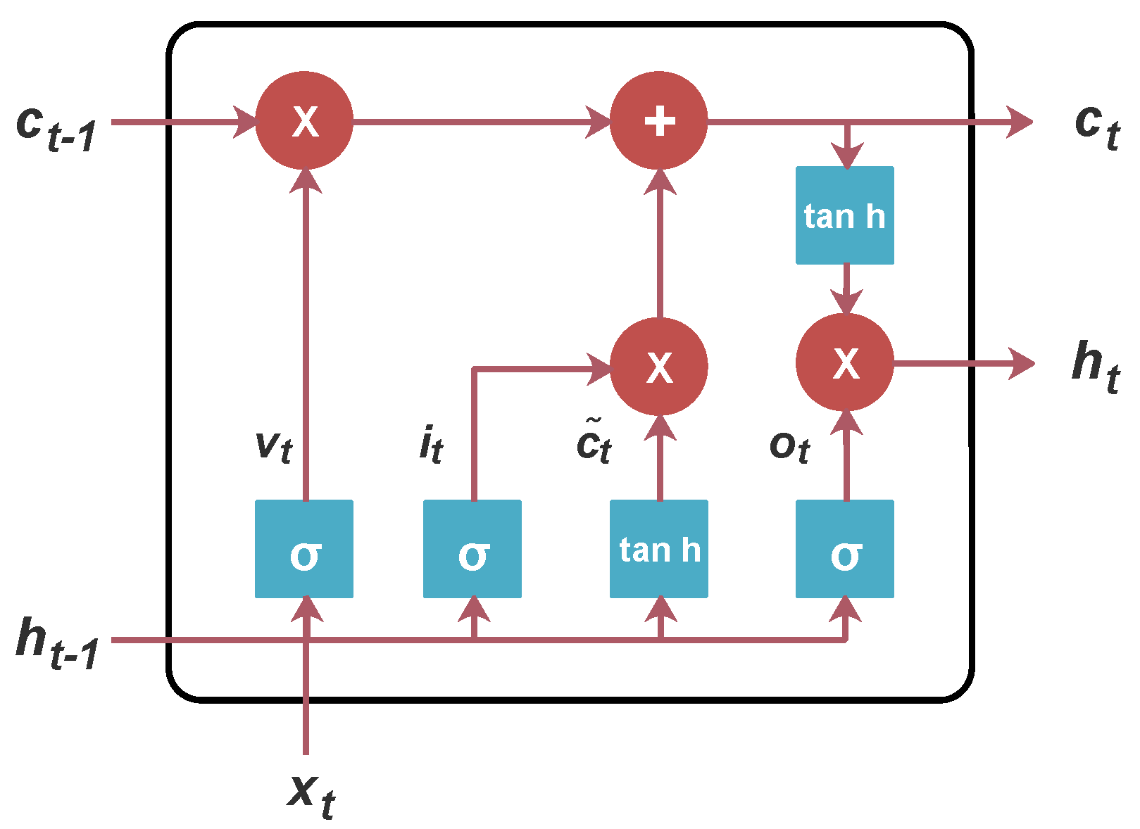
Deep learning models have continuously advanced over many years. For applications in time-series data research, such approaches as the recurrent neural network (RNN) introduced the idea of a time sequence within a neural network structure design that enables it to handle time-series data analysis [36]. The subsequent development of LSTM cells extended this capability to enable the learning of long-term dependencies through gates that control the learning process [37]. With the option to add or delete information from this cell state, LSTM could then solve the vanishing-gradient problem that occurs in the standard RNN [38]. The cell computes a hidden state, or output vector $h_t$, of the LSTM cell, and then updates the cell state $c_t$ based on the previous cell ($c_{t-1}$, $h_{t-1}$) and the input sequence $x_t$ at time step t. The three gates of the input gate $i_t$, forget gate $v_t$, and output gate $o_t$ are the key components for the LSTM in learning long-term relations through the selection of which information should be kept. These LSTM gates are represented in Equation (9) and illustrated in Figure 4. The $c_0$ and $h_0$ coefficients are initialized with the value of 0, and the operator ∘ represents an element-wise product. The term ${\tilde{c}}_t$ is the cell input activation vector, and $\sigma$ and tanh are the sigmoid and hyperbolic tangent functions, respectively. The training objective is to optimize W, R, and the b parameter, where W and R are the input and recurrent cell weights, respectively, while b is the bias vector:

$$\begin{array}{c}\hfill \begin{array}{c}{v}_t=\sigma \left(W_f{x}_t+U_f{h}_{t-1}+b_f\right)\hfill \\ i_t=\sigma \left(W_i{x}_t+U_i{h}_{t-1}+b_i\right)\hfill \\ o_t=\sigma \left(W_o{x}_t+U_o{h}_{t-1}+b_o\right)\hfill \\ {\tilde{c}}_t=tanh\left(W_c{x}_t+U_c{h}_{t-1}+b_c\right)\hfill \\ c_t=f_t\circ c_{t-1}+i_t\circ {\tilde{c}}_t\hfill \\ h_t=o_t\circ tanh\left(c_t\right)\hfill \end{array}\end{array}$$

(9)

7.2. Denoising and Latent Feature Extraction

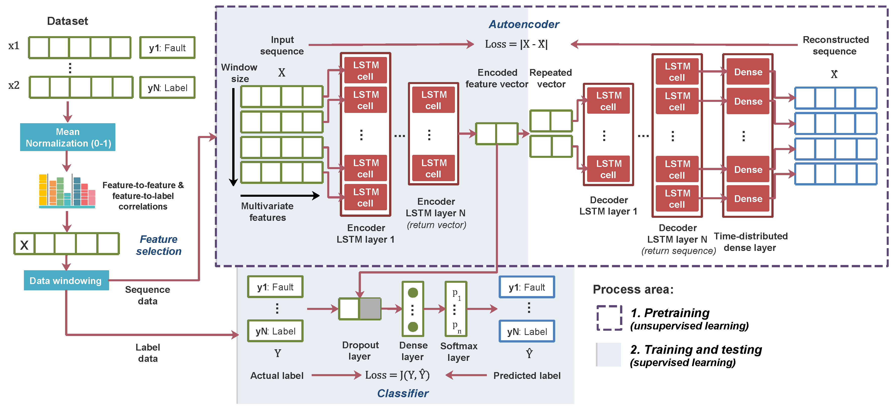
The schema of the proposed fault detection method is shown in Figure 5 and is presented as an LSTM-based autoencoder model or LSTM-AE. AEs are used in representation learning with the objective of reconstructing the input data $\mathbf{x}$ from an encoded representation. The components of the AE include an encoder $e_{\varphi }$ and a decoder $d_{\theta }$ as expressed in Equation (10). The process of pre-training is described in Algorithm 3 with lines 4–9. The encoder focuses on the task to learn the prominent characteristics and extract the encoded features $\mathbf{h}$ [39]. The decoder reconstructs the input from the encoded features ${\mathbf{x}}^{\prime }$. Because the encoder returns a vector, we require a repeated vector function to convert the vector into sequence data, so that it can input into the decoder. The encoder and decoder feature a symmetric architecture. The reconstruction error measured with the mean squared error is expressed in Equation (11). The model parameter optimization is based on the error via the backpropagation algorithm. An AE can handle noisy data because it can extract latent features from the data if it is clean or noisy [40]. Our LSTM-based autoencoder basically is a sequence-to-sequence model that reconstruct time-series sequences [41]. The LSTM-AE provides the functionality of the feature extractor during the pre-training phase, which provides the initial weight to the model [42]. Therefore, the classifier has an optimized initial weight for training the model:

$$\begin{array}{c}\hfill e_{\varphi }\left(\mathbf{x}\right)=\mathbf{h}\\ \hfill d_{\theta }\left(\mathbf{h}\right)={\mathbf{x}}^{\prime }\end{array}$$

(10)

$$\begin{array}{c}\hfill L_{\mathrm{AE}}(\theta ,\varphi )=\frac{1}{n}\sum _{i=1}^n{({\mathbf{x}}_i-d_{\theta }\left(e_{\varphi }\left({\mathbf{x}}_i\right)\right))}^2\end{array}$$

(11)

Algorithm 3 Pre-training-Training of the LSTM-AE.

Input Number of epochs, Feature selected data $\mathcal{X}$    Output Trained classifier $CLF$  1: Calculate mean and normalize $\mathbf{X}$  2: Data windowing $\mathcal{X}\to \mathbf{X}$  3: Parameter initialization $\theta ,\varphi$    ▹ Pre-training Autoencoder  4: Build autoencoder model $AE$  5: for all epochs do  6:     Calculate encoder output vector $\mathbf{h}$  7:     Calculate reconstructed output ${\mathbf{x}}^{\prime }$  8:     Calculate reconstruction cost $L_{\mathrm{AE}}(\theta ,\varphi )$  9:     Update parameter $\theta ,\varphi$ via backpropagation    ▹ Training Classifier 10: Build $CLF$ model from encoder and classifier layer 11: for all epochs do 12:     Calculate dense layer output vector $\mathbf{z}$ 13:     Calculate class probability $s{\left(\mathbf{z}\right)}_i$ 14:     Calculate classification error $L_{\mathrm{CLF}}(\theta ,\sigma )$ 15:     Update parameter $\theta ,W$ via backpropagation

7.3. Fault Classification

After pre-training the LSTM-AE, the encoder is merged and trained with a dropout layer, a fully connected, or dense layer [43], and a softmax classifier layer. The dropout is a regularization method where random neurons are ignored during training so that the network can obtain better generalization and prevent overfitting [44]. The softmax classifier layer [45] assigns the transformed vector into the predicted classes and its distribution. The process of training is described in Algorithm 3 with lines 10–15. This classifier model undergoes supervised training using labeled data, and a categorical cross-entropy loss [46] optimizes the dense weight and encoder parameters via the backpropagation algorithm, as expressed in Equation (14):

$$\begin{array}{c}\hfill \begin{array}{c}{z}_t=R(W_i{h}_t+b_i)\hfill \\ R\left(x\right)=max(0,x)\hfill \end{array}\end{array}$$

(12)

$$s{\left(\mathbf{z}\right)}_i=\frac{e^{z_i}}{{\sum }_j^c{e}^{z_j}}\mathrm{for}i=1,\dots ,c$$

(13)

$$L_{\mathrm{CLF}}(\theta ,\sigma )=-\sum _i^c{\mathbf{y}}_{i}log\left(s{\left(\mathbf{z}\right)}_i\right)$$

(14)

8. Performance Evaluation

8.1. Experimental Setup

We performed experiments using three devices to act as a sensor pool, edge server, and cloud server. The sensor pool sends the data to the target server, and either the edge or cloud server collects the data and performs the fault detection with the trained model. We implemented the CRFS algorithm using JmetalPy [47], and the fault detection model was implemented in Tensorflow [48] with Keras [49] for the high-level API to build the model. The experiments were evaluated through the accuracy (0–1), detection time (ms) that maintains the total of data transmission time and model prediction time, and packet size (KB).

Table 4. Experimental parameters.

Parameter		Value
CRFS	Population and Offspring size	100
	Mutation	Bit-flip ($1/n$) [50]
	Crossover	Single-point ($0.9$) [51]
	Selection	Binary tournament [52]
	Weights	$w_{co{r}_o}=0.4,w_{co{r}_f}=0.4,w_{n{b}_f}=0.2$
	Iterations	25,000
LSTM-AE	Test data ratio	0.2
	Encoder and Decoder units	[64, 32, 16] and [16, 32, 64]
	Encoded features	8
	Dense neurons	8
	Dropout	0.3
	Window size	3
	Learning rate	0.001
	Optimizer	Adam [53]
	Batch	30
	Epochs	500
Device	Sensors pool	Ubuntu 16, Intel i3-6x, RAM 4GB
	Edge server	Windows 10, Intel i5-7x, RAM 4GB
	Cloud server	Digitalocean Ubuntu 18, 1TB Transfer

lists the parameters considered for these experiments.

8.2. Experiment on Feature Selection

8.2.1. Selected Features for Each Fault Type

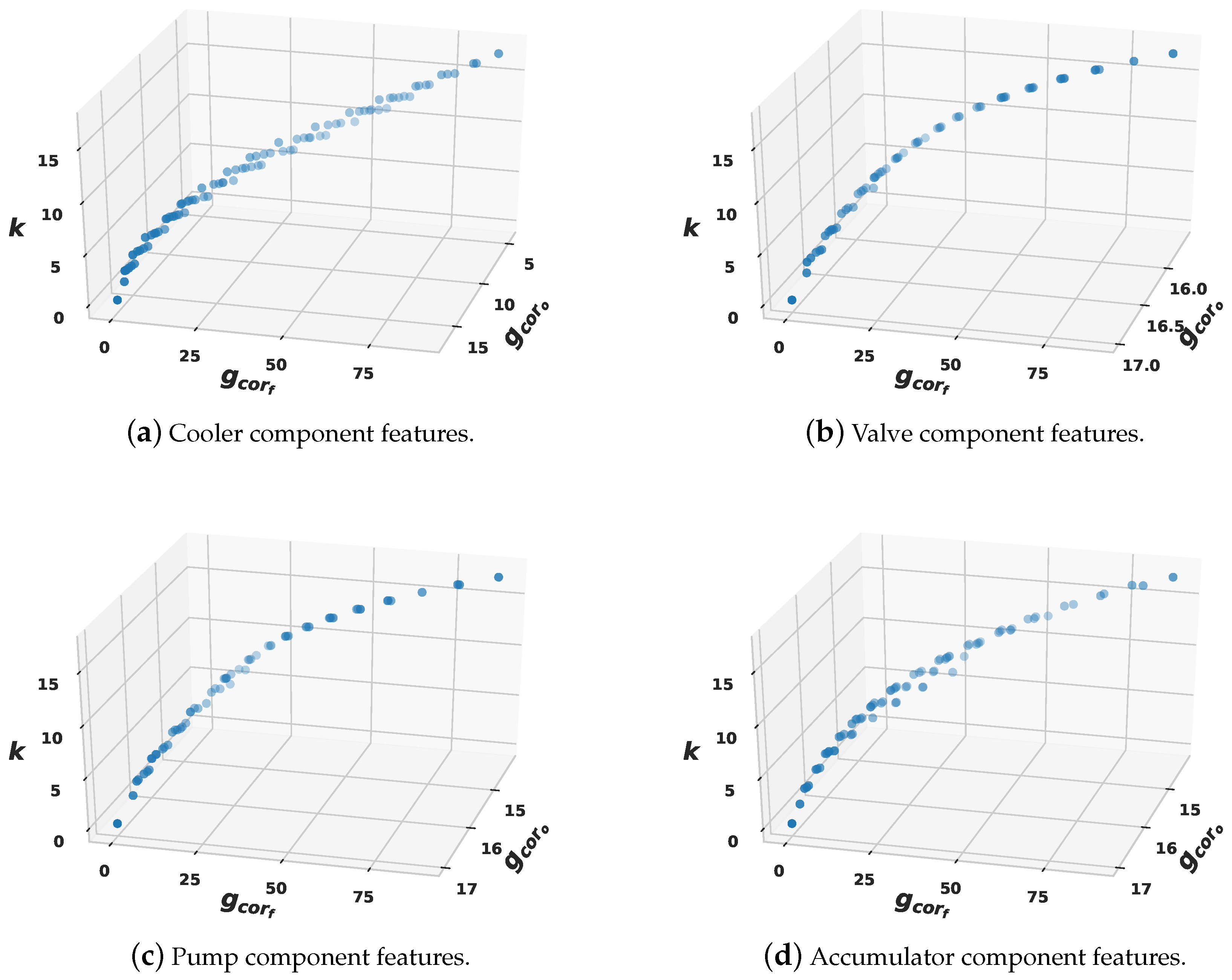
We evaluated the feature selection method with the results of the selected features for each fault type presented in

Table 5. Selected features for each fault type.

Component	Selected Sensor Feature	${\mathit{g}}_{{\mathbf{cor}}_{\mathit{o}}}$	${\mathit{g}}_{{\mathbf{cor}}_{\mathit{f}}}$	k
Cooler	PS5, PS6, TS1, TS2, TS4	12.127	9.958	5
Valve	EPS1, FS1, PS1, PS3, PS4, SE, VS1	15.855	12.516	7
Pump	EPS1, FS1, PS1, PS2, PS3, PS4, SE	14.551	13.558	7
Accumulator	EPS1, PS1, PS5, PS6, CE, CP	15.723	8.736	6

. Figure 6 shows the non-dominated individuals that spread across the Pareto front. Among these, we selected the best according to the lowest weighted and scaled objective value. These features are those that fulfill the CRFS objectives such that they have a high correlation to the label and low redundancy with the other features. From these results, the CRFS reduces the features by 63%, from 17 initially into 5–7 features. The Cooler and Accumulator obtain the smallest number of selected features. Thus, although we did not incorporate domain knowledge of the hydraulic system and its fault correlations, the CRFS finds the sensor features that relate to a fault in certain components. The Valve and Pump components share nearly similar features, which suggests that these have a strong fault correlation. Therefore, these selected features are used for the subsequent experiment.

8.2.2. Performance of Server Types

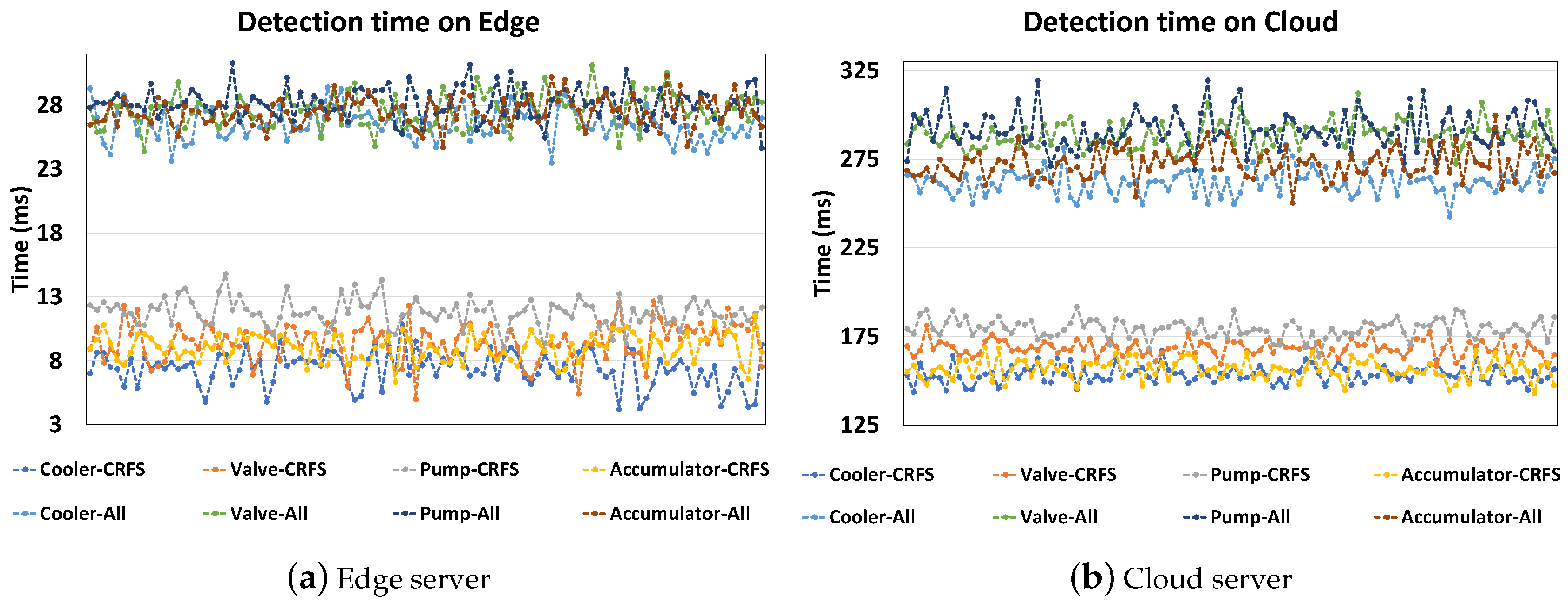
We evaluated the usage of the CRFS in different architectures, with results listed in

Table 6. Performance of server types.

Server	Component	Features	Detection Time (ms)	Packet Size (KB)
Edge	Cooler	CRFS (5)	7.31	95.9
		All (17)	26.74	343.78
	Valve	CRFS (7)	9.53	194.16
		All (17)	27.63	343.78
	Pump	CRFS (7)	11.85	240.56
		All (17)	28.21	343.78
	Accumulator	CRFS (6)	8.99	189.32
		All (17)	27.45	343.78
Cloud	Cooler	CRFS (5)	152.56	95.9
		All (17)	261.52	343.78
	Valve	CRFS (7)	168.75	194.16
		All (17)	288.35	343.78
	Pump	CRFS (7)	180.14	240.56
		All (17)	293.11	343.78
	Accumulator	CRFS (6)	157.13	189.32
		All (17)	272.52	343.78

and presented in Figure 7. The detection time by the edge server is below 30 ms, even when dealing with all features, while the detection time by the cloud server exceeds 200 ms. The packet size is calculated from the total of the selected features packet size. The Cooler component maintains the smallest packet size because its selected features are those with a small sampling rate. The difference between the detection times by the cloud is large (i.e., unstable) and of at least 10 ms, while in the edge it is at least 1–2 ms. The cloud has a high detection time because of the long-distance connection with a significant amount of data being sent. These results suggest that edge computing is a suitable architecture to apply to fault detection systems by providing computing resources near the data sources while maintaining low latency. Hence, an edge server is incorporated in the next experiment.

8.2.3. Performance of Feature Selection

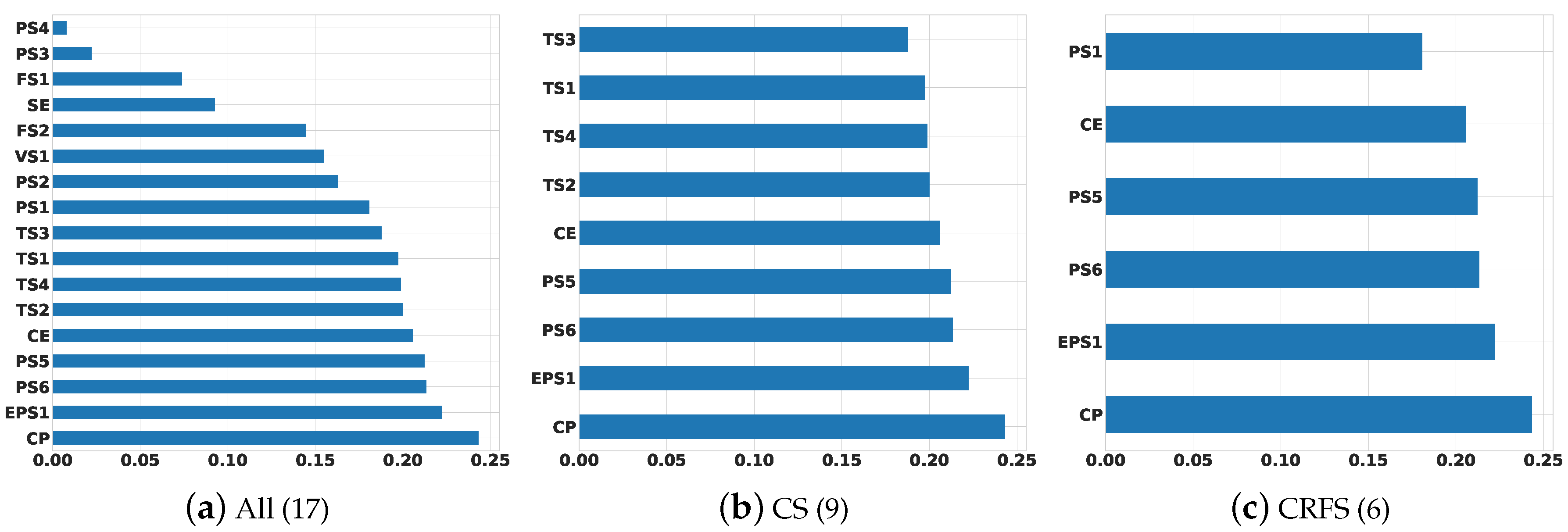
We evaluated the feature selection method on the fault detection model performance, with results listed in

Table 7. Performance of feature selection.

Component	Features	Accuracy	Detection Time (ms)	Packet Size (KB)
Cooler	All (17)	1	26.74	343.78
	CS (9)	1	13.86	102.6
	CRFS (5)	1	7.31	95.9
Valve	All (17)	0.982	27.63	343.78
	CS (9)	0.969	14.37	246.02
	CRFS (7)	0.984	9.53	194.16
Pump	All (17)	0.991	28.21	343.78
	CS (9)	0.986	15.21	246.02
	CRFS (7)	1	11.85	240.56
Accumulator	All (17)	0.979	27.45	343.78
	CS (9)	0.968	14.23	144.78
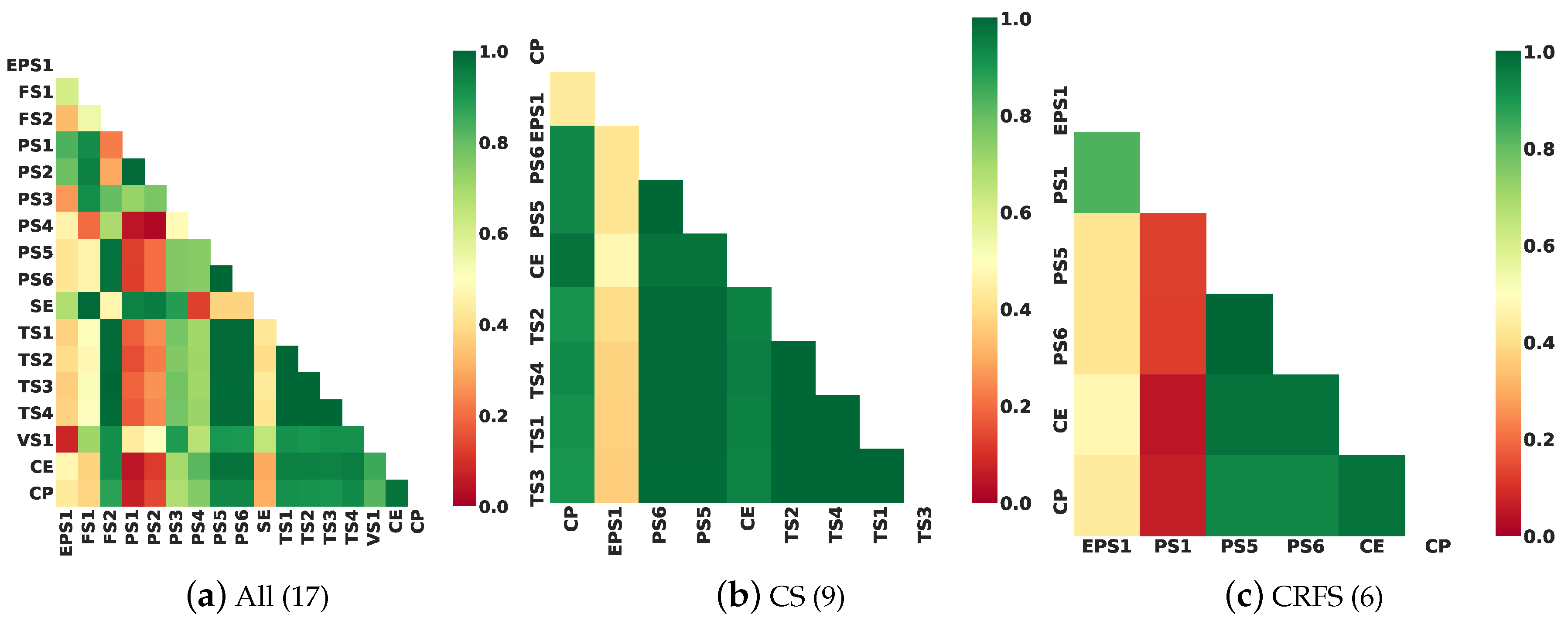
	CRFS (6)	0.989	8.99	189.32

. Although the CRFS maintains fewer selected features, it offers similar accuracy to the model that utilizes all features. The CRFS outperforms the accuracy of CS with its larger number of features. While CS maintains many features with a high correlation to the label, as seen in Figure 8, it also suffers by selecting redundant features, as also shown in Figure 9, with more green block feature-to-feature correlation indicating a high correlation between them. The CRFS maintains a high feature-to-label correlation, but also includes fewer redundant features. Thus, the CRFS should exhibit better feature learning on the model. In contrast, CS maintains a larger packet size and detection time with its larger number of selected features compared to that of CRFS.

8.3. Experiment with Fault Detection Methods

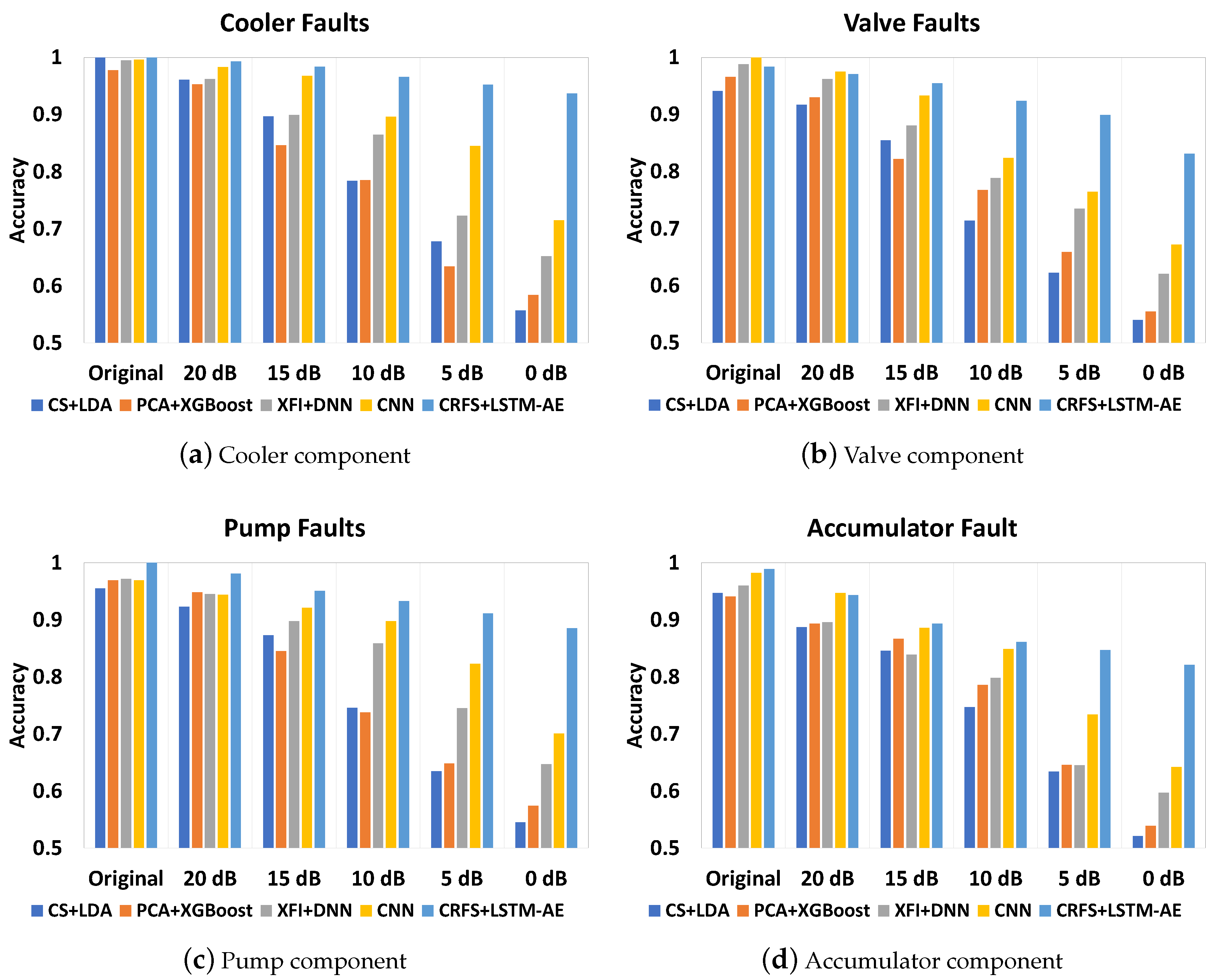
We measured the performance of our method and previous approaches spanning various noise levels, with results listed in

Table 8. Comparison to previous methods.

Component	Method	Accuracy						Detection Time (ms)
		Original	20 dB	15 dB	10 dB	5 dB	0 dB
Cooler	CS+LDA	1	0.961	0.897	0.784	0.678	0.557	3.75
	PCA+XGBoost	0.978	0.953	0.846	0.785	0.634	0.584	12.61
	XFI+DNN	0.995	0.962	0.899	0.865	0.723	0.652	13.44
	CNN	0.996	0.983	0.968	0.896	0.845	0.715	32.5
	CRFS+LSTM-AE	1	0.993	0.984	0.966	0.952	0.937	7.31
Valve	CS+LDA	0.941	0.917	0.855	0.714	0.623	0.540	4.64
	PCA+XGBoost	0.966	0.930	0.822	0.768	0.659	0.555	11.74
	XFI+DNN	0.988	0.962	0.881	0.789	0.735	0.621	12.89
	CNN	1	0.975	0.933	0.824	0.765	0.672	30.15
	CRFS+LSTM-AE	0.984	0.971	0.955	0.924	0.899	0.831	9.53
Pump	CS+LDA	0.955	0.923	0.873	0.746	0.635	0.545	5.13
	PCA+XGBoost	0.969	0.948	0.845	0.738	0.648	0.574	12.16
	XFI+DNN	0.972	0.945	0.898	0.859	0.745	0.647	14.19
	CNN	0.969	0.944	0.921	0.898	0.823	0.701	29.98
	CRFS+LSTM-AE	1	0.981	0.951	0.933	0.911	0.885	11.85
Accumulator	CS+LDA	0.947	0.887	0.846	0.747	0.634	0.521	3.61
	PCA+XGBoost	0.941	0.893	0.867	0.786	0.646	0.539	12.33
	XFI+DNN	0.960	0.896	0.839	0.798	0.645	0.597	15.18
	CNN	0.982	0.947	0.886	0.849	0.734	0.642	31.21
	CRFS+LSTM-AE	0.989	0.943	0.893	0.861	0.847	0.821	8.99

and presented in Figure 10. XFI, CS, and CRFS are based on a one-time analysis during offline learning that defines the selected features. CRFS maintains smaller packet sizes compared to other methods that require all features to be transmitted before they can be processed, so they have a maximum packet size of 343.78 KB. Another advantage of CRFS over XFI and CS is that defining the number of selected features is not required because this is set as an objective. CS+LDA and XFI+DNN have another drawback in that they must generate statistical features on every sample, requiring more time and computational resources. CRFS uses the raw feature subset rather than statistical features, thus CRFS can define the sensor to send only those selected features, while XFI and CS still need to retrieve all of the data to be converted into statistical features before filtering. Due to the model simplicity in CS+LDA as a traditional machine learning approach, this method could maintain the lowest detection time. XFI-XGBoost is also a lightweight model but suffers from the need to transform all features into principal components, which is time-consuming.

A comparison of the complexity between the deep learning-based fault detection models is listed in

Table 9. Complexity of the deep learning models.

Deep Learning Model	Total Parameters	Model Size (KB)
DNN [23]	52,351	227
CNN [27]	16,189,496	63,275
LSTM-AE (CLF)	34,584	169

and suggests that the classifier part of our proposed LSTM-AE model maintains the least number of parameters and smallest model size. Because the LSTM-AE classifier features a lower complexity than the DNN and CNN architectures used in previous works, this approach also supports real-time predictions at the edge server. The CRFS+LSTM-AE obtains the second-lowest detection time. As the detection times of every algorithm are below 50 ms, this approach enables edge computing that is capable of real-time detection. In addition, the CRFS+LSTM-AE has the smallest packet size among these experiments. The accuracy of the CRFS+LSTM-AE also outperforms the others, even when processing data with a signal-to-noise ratio of 0 dB and above. The CNN also works well in noisy data, followed by the DNN, while XGBoost and LDA do not perform well.

9. Conclusions

The challenges in fault detection for hydraulic systems include maintaining real-time fault detection, learning multivariate time-series sensor data, and handling noisy data. To address these issues, we propose a real-time and robust fault detection approach through cooperation between cloud and edge servers. The cloud conducts feature selection and offline learning, while the edge processes online detection near the data source to reduce latency and transmission costs. We outline a new method leveraging GA-based feature selection to identify feature-to-label correlations and feature-to-feature redundancies. By using fewer important features that are transmitted to the edge and processed, detection time is reduced, and model performance is improved. Finally, we describe an LSTM-AE as a robust fault detection model that fully uses temporal information on time-series sensor data that is capable of handling noisy data. The experimental results suggested that our method outperforms previous approaches as we obtain lower detection times, higher accuracies, and more robust performance in the presence of noisy data. With a 63% reduction in features, from 17 to 5–7, our model still attains high accuracy above 98% while being robust to noisy data when the signal-to-noise ratio is approximately 0 dB. Our method also maintains low detection times with an average of 9.42 ms and reduces the packet size to 179.98 KB from a maximum of 343.78 KB.

For future work, we will first consider other deep learning models, such as CNN combined with LSTM, to offer a better learning model for spatio-temporal data. Then, we will apply this proposed method to other real-world datasets or systems. Finally, we will consider incomplete sensor data issues that could arise from hardware malfunctions or during device replacement.

References

- Fu, X.B.; Liu, B.; Zhang, Y.C.; Lian, L.N. Fault diagnosis of hydraulic system in large forging hydraulic press. Measurement 2014, 49, 390–396. [Google Scholar] [CrossRef]
- Jegadeeshwaran, R.; Sugumaran, V. Fault diagnosis of automobile hydraulic brake system using statistical features and support vector machines. Mech. Syst. Signal Process. 2015, 52, 436–446. [Google Scholar] [CrossRef]
- He, X. Fault diagnosis approach of hydraulic system using FARX model. Procedia Eng. 2011, 15, 949–953. [Google Scholar] [CrossRef]
- Lu, C.; Wang, S.; Wang, X. A multi-source information fusion fault diagnosis for aviation hydraulic pump based on the new evidence similarity distance. Aerosp. Sci. Technol. 2017, 71, 392–401. [Google Scholar] [CrossRef]
- Liu, X.; Tian, Y.; Lei, X.; Liu, M.; Wen, X.; Huang, H.; Wang, H. Deep forest based intelligent fault diagnosis of hydraulic turbine. J. Mech. Sci. Technol. 2019, 33, 2049–2058. [Google Scholar] [CrossRef]
- Alsyouf, I. The role of maintenance in improving companies’ productivity and profitability. Int. J. Prod. Econ. 2007, 105, 70–78. [Google Scholar] [CrossRef]
- Gao, Z.; Ding, S.X.; Cecati, C. Real-time fault diagnosis and fault-tolerant control. IEEE Trans. Ind. Electron. 2015, 62, 3752–3756. [Google Scholar] [CrossRef]
- Xu, Y.; Sun, Y.; Wan, J.; Liu, X.; Song, Z. Industrial big data for fault diagnosis: Taxonomy, review, and applications. IEEE Access 2017, 5, 17368–17380. [Google Scholar] [CrossRef]
- Tan, Y.L.; Sehgal, V.; Shahri, H.H. Sensoclean: Handling Noisy and Incomplete Data in Sensor Networks Using Modeling. 2005. Available online: https://pdfs.semanticscholar.org/d3d4/91fe3ea49c5d03b98b6fc517eee2bd27cabf.pdf (accessed on 30 July 2020).
- Xu, L.D.; Xu, E.L.; Li, L. Industry 4.0: State of the art and future trends. Int. J. Prod. Res. 2018, 56, 2941–2962. [Google Scholar] [CrossRef]
- Zhong, R.Y.; Xu, X.; Klotz, E.; Newman, S.T. Intelligent manufacturing in the context of industry 4.0: A review. Engineering 2017, 3, 616–630. [Google Scholar] [CrossRef]
- Wan, J.; Yang, J.; Wang, Z.; Hua, Q. Artificial intelligence for cloud-assisted smart factory. IEEE Access 2018, 6, 55419–55430. [Google Scholar] [CrossRef]
- Shi, W.; Cao, J.; Zhang, Q.; Li, Y.; Xu, L. Edge computing: Vision and challenges. IEEE Internet Things J. 2016, 3, 637–646. [Google Scholar] [CrossRef]
- Bangui, H.; Rakrak, S.; Raghay, S.; Buhnova, B. Moving to the edge-cloud-of-things: Recent advances and future research directions. Electronics 2018, 7, 309. [Google Scholar] [CrossRef]
- Helwig, N.; Pignanelli, E.; Schütze, A. Condition monitoring of a complex hydraulic system using multivariate statistics. In Proceedings of the 2015 IEEE International Instrumentation and Measurement Technology Conference (I2MTC), Pisa, Italy, 11–14 May 2015; pp. 210–215. [Google Scholar]
- Park, D.; Kim, S.; An, Y.; Jung, J.Y. Lired: A light-weight real-time fault detection system for edge computing using lstm recurrent neural networks. Sensors 2018, 18, 2110. [Google Scholar] [CrossRef]
- Syafrudin, M.; Fitriyani, N.L.; Alfian, G.; Rhee, J. An affordable fast early warning system for edge computing in assembly line. Appl. Sci. 2019, 9, 84. [Google Scholar] [CrossRef]
- Li, L.; Ota, K.; Dong, M. Deep learning for smart industry: Efficient manufacture inspection system with fog computing. IEEE Trans. Ind. Inform. 2018, 14, 4665–4673. [Google Scholar] [CrossRef]
- Wang, T.; Chen, Y.; Qiao, M.; Snoussi, H. A fast and robust convolutional neural network-based defect detection model in product quality control. Int. J. Adv. Manuf. Technol. 2018, 94, 3465–3471. [Google Scholar] [CrossRef]
- Schneider, T.; Helwig, N.; Schütze, A. Industrial condition monitoring with smart sensors using automated feature extraction and selection. Meas. Sci. Technol. 2018, 29, 094002. [Google Scholar] [CrossRef]
- Nanopoulos, A.; Alcock, R.; Manolopoulos, Y. Feature-based classification of time-series data. Int. J. Comput. Res. 2001, 10, 49–61. [Google Scholar]
- Li, Y.R.; Xiang, G.B. A linear discriminant analysis classification algorithm based on Mahalanobis distance. Comput. Simul. 2006, 8, 86–88. [Google Scholar]
- Prakash, J.; Kankar, P. Health prediction of hydraulic cooling circuit using deep neural network with ensemble feature ranking technique. Measurement 2020, 151, 107225. [Google Scholar] [CrossRef]
- Chen, T.; Guestrin, C. Xgboost: A scalable tree boosting system. In Proceedings of the 22nd Acm Sigkdd International Conference on Knowledge Discovery and Data Mining, San Francisco, CA, USA, 13–17 August 2016; pp. 785–794. [Google Scholar]
- Lei, Y.; Jiang, W.; Jiang, A.; Zhu, Y.; Niu, H.; Zhang, S. Fault diagnosis method for hydraulic directional valves integrating PCA and XGBoost. Processes 2019, 7, 589. [Google Scholar] [CrossRef]
- Abdi, H.; Williams, L.J. Principal component analysis. Wiley Interdiscip. Rev. Comput. Stat. 2010, 2, 433–459. [Google Scholar] [CrossRef]
- König, C.; Helmi, A.M. Sensitivity Analysis of Sensors in a Hydraulic Condition Monitoring System Using CNN Models. Sensors 2020, 20, 3307. [Google Scholar] [CrossRef] [PubMed]
- Yuan, Y.; Ma, G.; Cheng, C.; Zhou, B.; Zhao, H.; Zhang, H.T.; Ding, H. A general end-to-end diagnosis framework for manufacturing systems. Nat. Sci. Rev. 2020, 7, 418–429. [Google Scholar] [CrossRef]
- LeCun, Y.; Bengio, Y. Convolutional networks for images, speech, and time series. Handb. Brain Theory Neural Netw. 1995, 3361, 1995. [Google Scholar]
- Leevy, J.L.; Khoshgoftaar, T.M.; Bauder, R.A.; Seliya, N. A survey on addressing high-class imbalance in big data. J. Big Data 2018, 5, 42. [Google Scholar] [CrossRef]
- Kramer, O. Genetic Algorithm Essentials. In Studies in Computational Intelligence; Springer: Cham, Switzerland, 2017. [Google Scholar]
- Yang, J.; Honavar, V. Feature Subset Selection Using a Genetic Algorithm. In Feature Extraction, Construction and Selection: A Data Mining Perspective; Springer: Boston, MA, USA, 1998; pp. 117–136. [Google Scholar] [CrossRef]
- Deb, K.; Pratap, A.; Agarwal, S.; Meyarivan, T. A fast and elitist multiobjective genetic algorithm: NSGA-II. IEEE Trans. Evol. Comput. 2002, 6, 182–197. [Google Scholar] [CrossRef]
- Yu, L.; Liu, H. Efficient feature selection via analysis of relevance and redundancy. J. Mach. Learn. Res. 2004, 5, 1205–1224. [Google Scholar]
- Benesty, J.; Chen, J.; Huang, Y.; Cohen, I. Pearson correlation coefficient. In Noise Reduction in Speech Processing; Springer: Berlin, Germany, 2009; pp. 1–4. [Google Scholar]
- Dorffner, G. Neural Networks for Time Series Processing. Neural Netw. World 1996, 6, 447–468. [Google Scholar]
- Hochreiter, S.; Schmidhuber, J. Long short-term memory. Neural Comput. 1997, 9, 1735–1780. [Google Scholar] [CrossRef]
- Hochreiter, S. The vanishing gradient problem during learning recurrent neural nets and problem solutions. Int. J. Uncertain. Fuzziness Knowl.-Based Syst. 1998, 6, 107–116. [Google Scholar] [CrossRef]
- Wang, Y.; Yao, H.; Zhao, S. Auto-Encoder Based Dimensionality Reduction. Neurocomputing 2016, 184, 232–242. [Google Scholar] [CrossRef]
- Vincent, P.; Larochelle, H.; Bengio, Y.; Manzagol, P.A. Extracting and composing robust features with denoising autoencoders. In Proceedings of the 25th International Conference on Machine Learning, Helsinki, Finland, 5–9 July 2008; pp. 1096–1103. [Google Scholar]
- Sutskever, I.; Vinyals, O.; Le, Q.V. Sequence to sequence learning with neural networks. In Advances in Neural Information Processing Systems; Curran Associates, Inc.: Red Hook, NY, USA, 2014; pp. 3104–3112. [Google Scholar]
- Erhan, D.; Courville, A.; Bengio, Y.; Vincent, P. Why does unsupervised pre-training help deep learning? In Proceedings of the Thirteenth International Conference on Artificial Intelligence and Statistics, Sardinia, Italy, 13–15 May 2010; pp. 201–208. [Google Scholar]
- Schmidhuber, J. Deep learning in neural networks: An overview. Neural Netw. 2015, 61, 85–117. [Google Scholar] [CrossRef] [PubMed]
- Srivastava, N.; Hinton, G.; Krizhevsky, A.; Sutskever, I.; Salakhutdinov, R. Dropout: A simple way to prevent neural networks from overfitting. J. Mach. Learn. Res. 2014, 15, 1929–1958. [Google Scholar]
- Bridle, J.S. Probabilistic interpretation of feedforward classification network outputs, with relationships to statistical pattern recognition. In Neurocomputing; Springer: Berlin, Germany, 1990; pp. 227–236. [Google Scholar]
- Janocha, K.; Czarnecki, W.M. On loss functions for deep neural networks in classification. arXiv 2017, arXiv:1702.05659. [Google Scholar] [CrossRef]
- Benitez-Hidalgo, A.; Nebro, A.J.; Garcia-Nieto, J.; Oregi, I.; Del Ser, J. jMetalPy: A python framework for multi-objective optimization with metaheuristics. Swarm Evol. Comput. 2019, 51, 100598. [Google Scholar] [CrossRef]
- Abadi, M.; Barham, P.; Chen, J.; Chen, Z.; Davis, A.; Dean, J.; Devin, M.; Ghemawat, S.; Irving, G.; Isard, M.; et al. Tensorflow: A system for large-scale machine learning. In Proceedings of the 12th Symposium on Operating Systems Design and Implementation, Savannah, GA, USA, 2–4 November 2016; pp. 265–283. [Google Scholar]
- Chollet, F. Keras. 2015. Available online: https://keras.io (accessed on 30 July 2020).
- Chicano, F.; Sutton, A.M.; Whitley, L.D.; Alba, E. Fitness probability distribution of bit-flip mutation. Evol. Comput. 2015, 23, 217–248. [Google Scholar] [CrossRef]
- Bridges, C.L.; Goldberg, D.E. An analysis of reproduction and crossover in a binary-coded genetic algorithm. Grefenstette 1987, 878, 9–13. [Google Scholar]
- Blickle, T. Tournament selection. Evol. Comput. 2000, 1, 181–186. [Google Scholar]
- Kingma, D.P.; Ba, J. Adam: A method for stochastic optimization. arXiv 2014, arXiv:1412.6980. [Google Scholar]
© 2020 by the authors. Licensee MDPI, Basel, Switzerland. This article is an open access article distributed under the terms and conditions of the Creative Commons Attribution (CC BY) license (http://creativecommons.org/licenses/by/4.0/).