The New Approach to Analysis of Thin Isotropic Symmetrical Plates
Abstract
1. Introduction
- Simplicity of structure modeling. Equations of equilibrium are solved once independently of the boundary conditions and solution remains unchanged throughout the calculation process. This allows the reduction of structure modeling to set kinematic and static boundary conditions in the separate points at the plate contour.
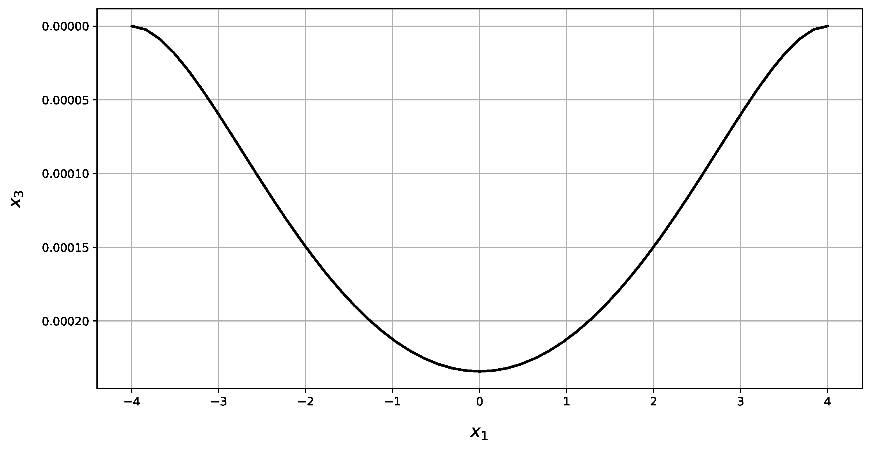
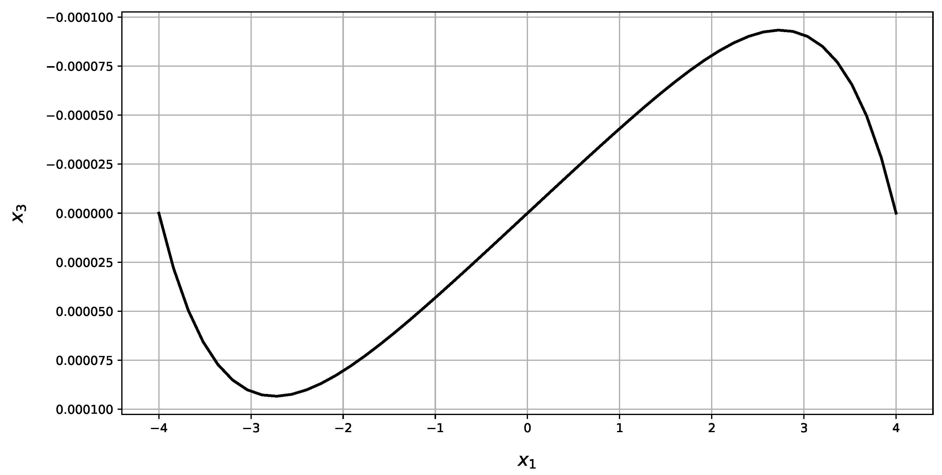
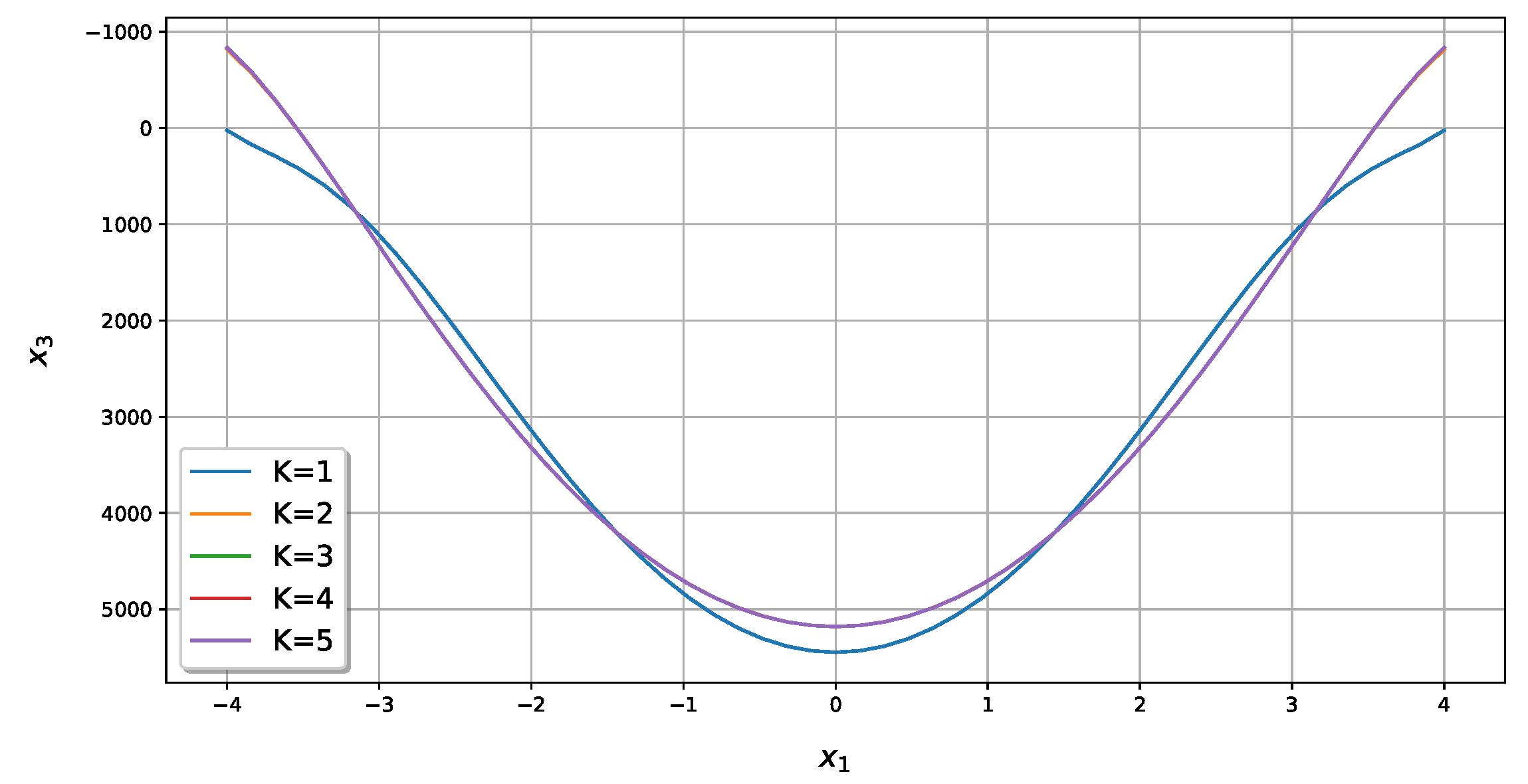
- Possibility to provide better accuracy in comparison with finite element method. It is achieved only by increasing of number of the approximations (parameter K) or replace nodes at the contour. This procedure is performed automatically with author’s program to solve of the plate structure.
- Possibility to define the load as a function of two variables. Because not all FEA programs provide such functionality, ABAQUS software have been chosen to compare the results.
- Possibility of implementing of suggested method in higher-order theory, say Mindlin-Reissner theory.
- Discretize of the structure into set of finite elements,
- Aggregate of this set into discrete structure,
- Introduce local and global coordinate system,
- Numerate of nodes. Solution of equilibrium equation can be obtained with given accuracy and it is independent of the number of approximations.
2. Literature Review of the Methods for Solving Plate Bending Problems
3. Materials and Methods
4. Results
- 1
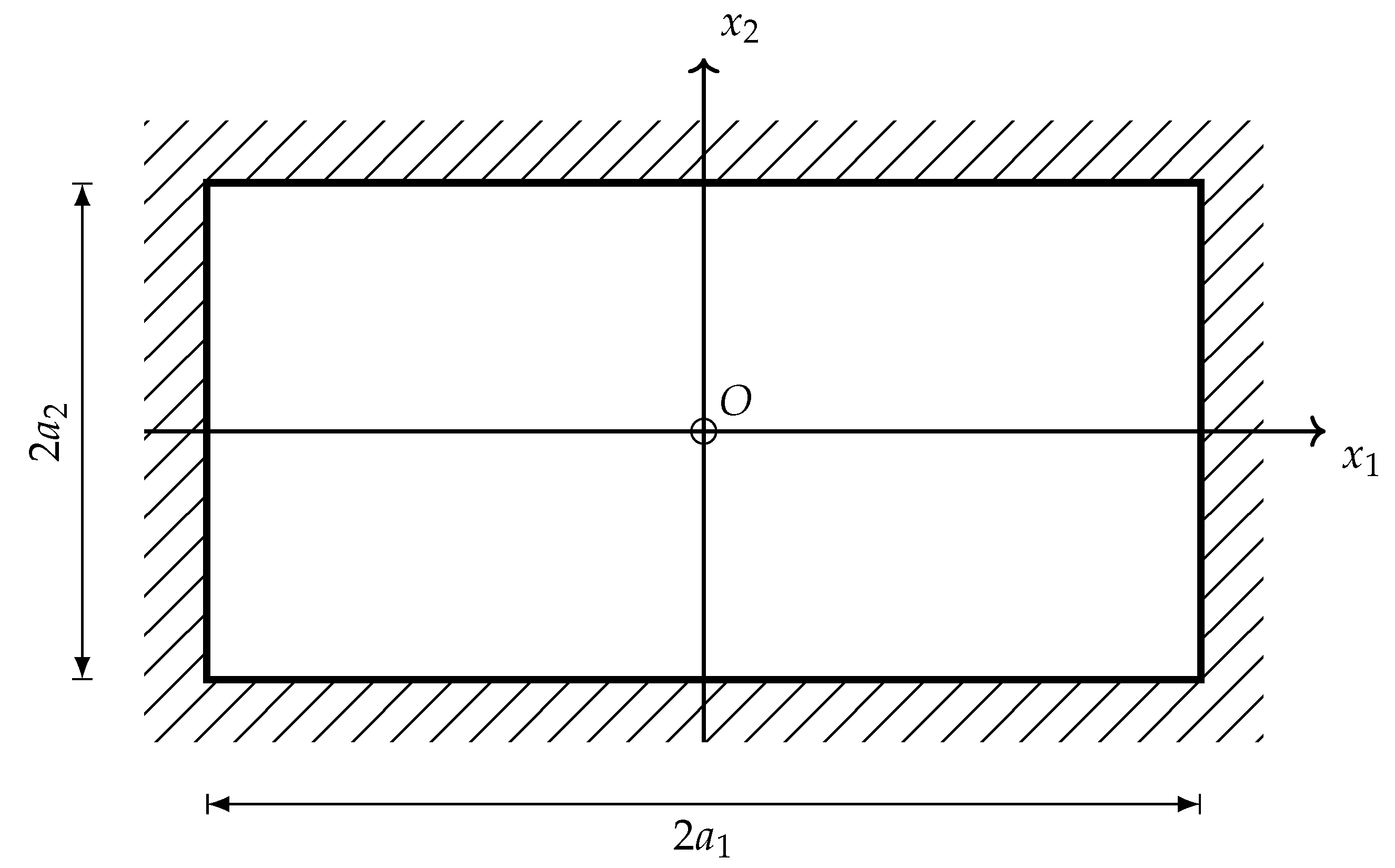
- Rectangular plate with two opposite edges simply supported and the other free,
- 2
- Rectangular plate simply supported at the contour,
- 3
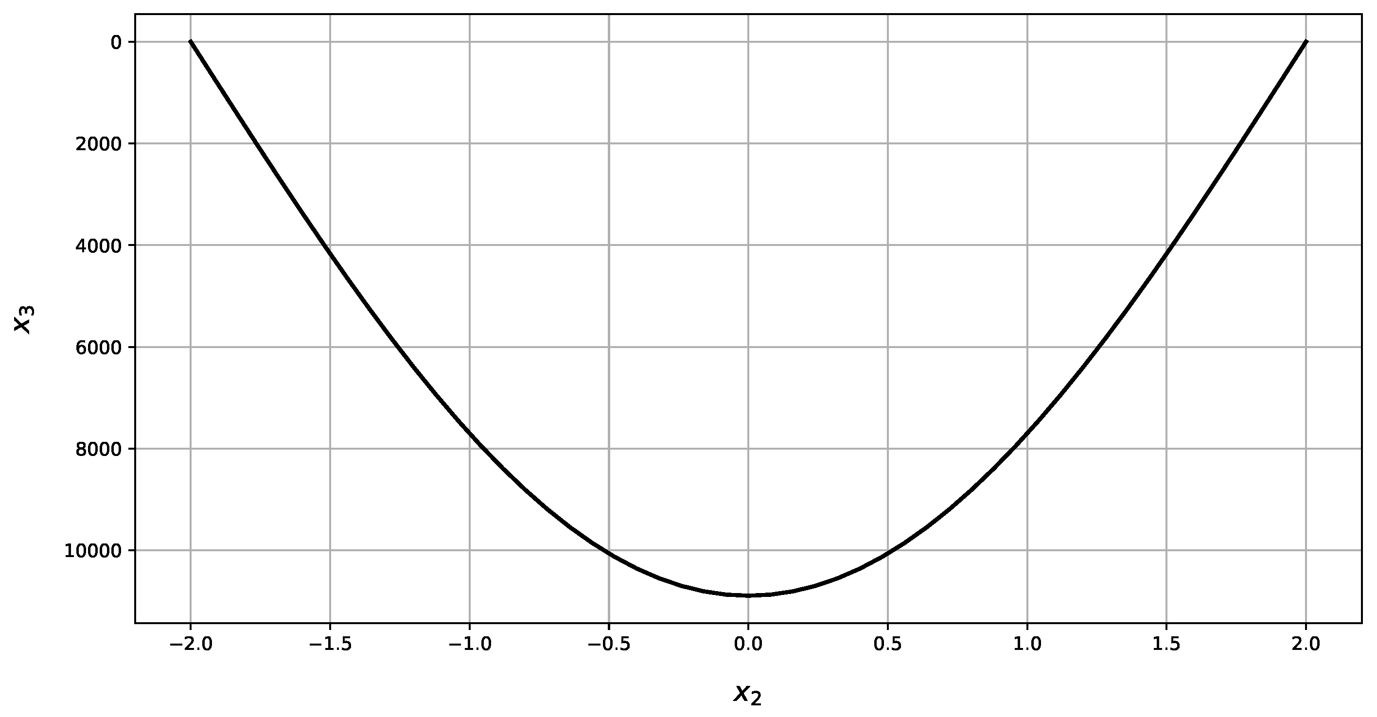
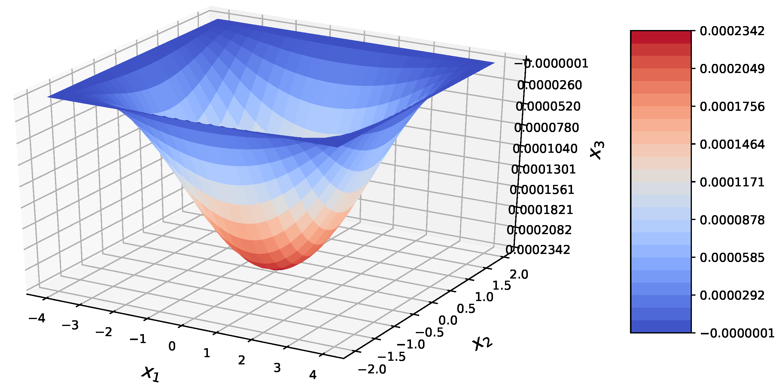
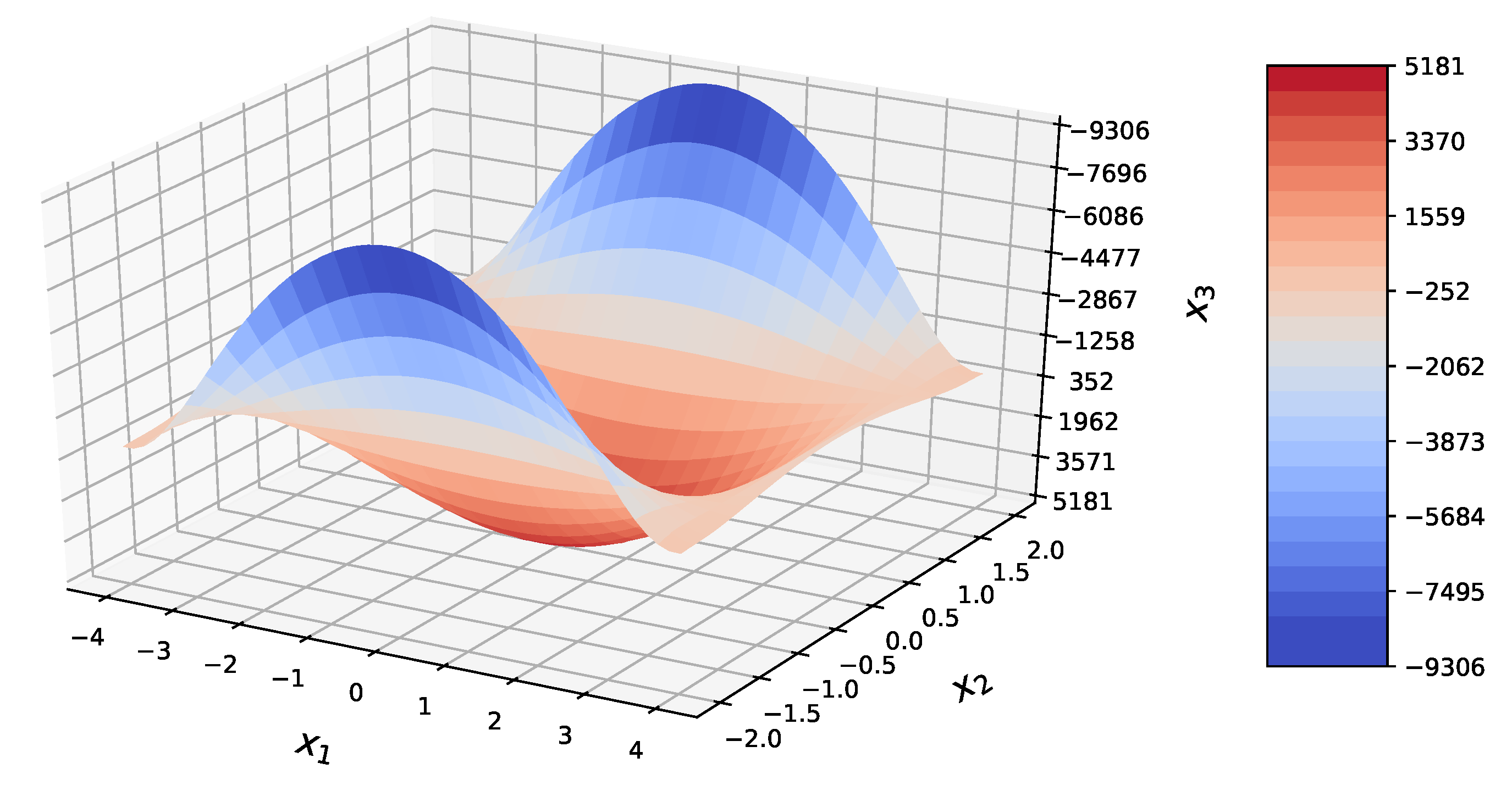
- Plate clamped at the contour.
| 0.0 | 0.8 | 1.6 | 2.4 | 3.2 | 4.0 | |
| 0.0 | 0.4 | 0.8 | 1.2 | 1.6 | 2.0 |
4.1. Rectangular Plate with Two Opposite Edges Simply Supported and the Other Free
4.2. Rectangular Plate Simply Supported at the Contour
4.3. Rectangular Plate Clamped at the Contour
5. Discussion
- Simplicity of structure modeling,
- Possibility to define static, kinematic and mixed boundary conditions,
- High accuracy and efficiency of calculation,
- Meshless approach for solving the problem.
- It cannot be used directly to solve fracture mechanics problems,
- It is worked for simply connected structures; for each additional contour, it is necessary to introduce the new block of basic functions,
- It gives good results for regular plates; plates with irregular geometry are solved with less accuracy,
- Unlike FEM, system matrix is consisted from zero and non-zero blocks.
- Presented method is based on Kirchhoff theory of the plates which is deformation theory of zeroth-order where deformations of a cross-section are omitted. Instead generalized shearing force as a sum of shearing forces and derivative of twisting moments is introduced.
- ABAQUS package is based on Mindlin plate theory which is deformation theory of first-order where deformations of a cross-section are taken into account. Twisting moments and shearing forces are independent ones. It is reason that obtained values of bending and twisting moments are different.
- Relatively small number of finite elements. The Student Edition of the ABAQUS package is restricted to 1000 nodes.
6. Conclusions
- to obtain with high accuracy particular solution of equilibrium equations at the separate surface nodes using boundary collocation method,
- to generate set of the initial points at the coordinate axis and then their distribution at the plate contour,
- to write boundary conditions at each edge nodes; number of these nodes always corresponds to number of unknown parameter of the model,
- to solve system of boundary equations,
- to calculate the desired magnitudes,
- to prepare the results.
- The mathematical model of thin isotropic plates is constructed. Basic shape and force functions are introduced.
- Within the model equilibrium equations are performed exactly.
- Expansion of the deflection within the area of the plate is obtained as sum of shape and force functions multiplied by unknown parameters.
- Displacements, slopes, moments and shearing forces are obtained using method of automatic differentiation. Union of presented relations create mathematical model of the plate.
- Within constructed model, a method to solving plate of arbitrary geometry have been suggested.
- All operations are performed automatically with author’s program.
- Effectiveness of method were illustrated at the examples of rectangular plates with various boundary conditions. Obtained results have been compared with numerical ones computed in ABAQUS package.
- With help of suggested method three kinds of the rectangular plates, namely: plate with two opposite edges simply supported and the other free; plate simply supported and clamped at the contour were solved. It has been shown that suggested method performs all boundary conditions. Finite element method performs exactly only kinematic ones. Static boundary conditions are performed with less accuracy.
Author Contributions
Funding
Conflicts of Interest
Abbreviations
| , , | Rectangular coordinates |
| h | Thickness of a plate |
| Intensity of a continuously distributed load | |
| E | Modulus of elasticity in tension and compression |
| Poisson’s ratio | |
| D | Flexural rigidity of a plate |
| w | Deflection of the plate |
| , | Slopes of the deflection |
| , | Bending moments per unit length of sections of a plate perpendicular to and axes, respectively |
| Twisting moment per unit length of sections of a plate perpendicular to axis | |
| , | Shearing forces parallel to axis per unit length of sections of a plate perpendicular to and axes, respectively |
| , | Generalized shearing forces parallel to axis per unit length of sections of a plate perpendicular to and axes |
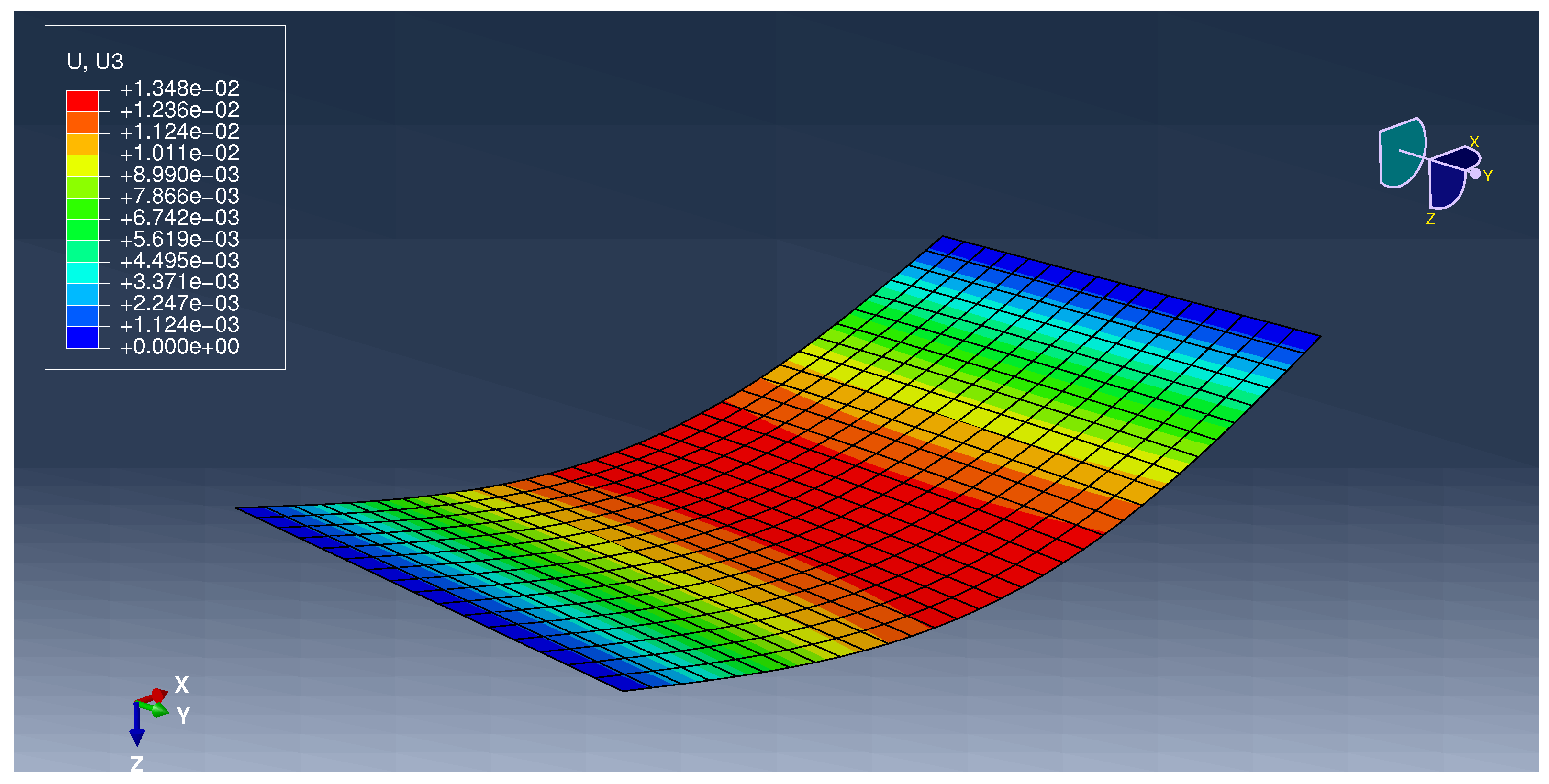
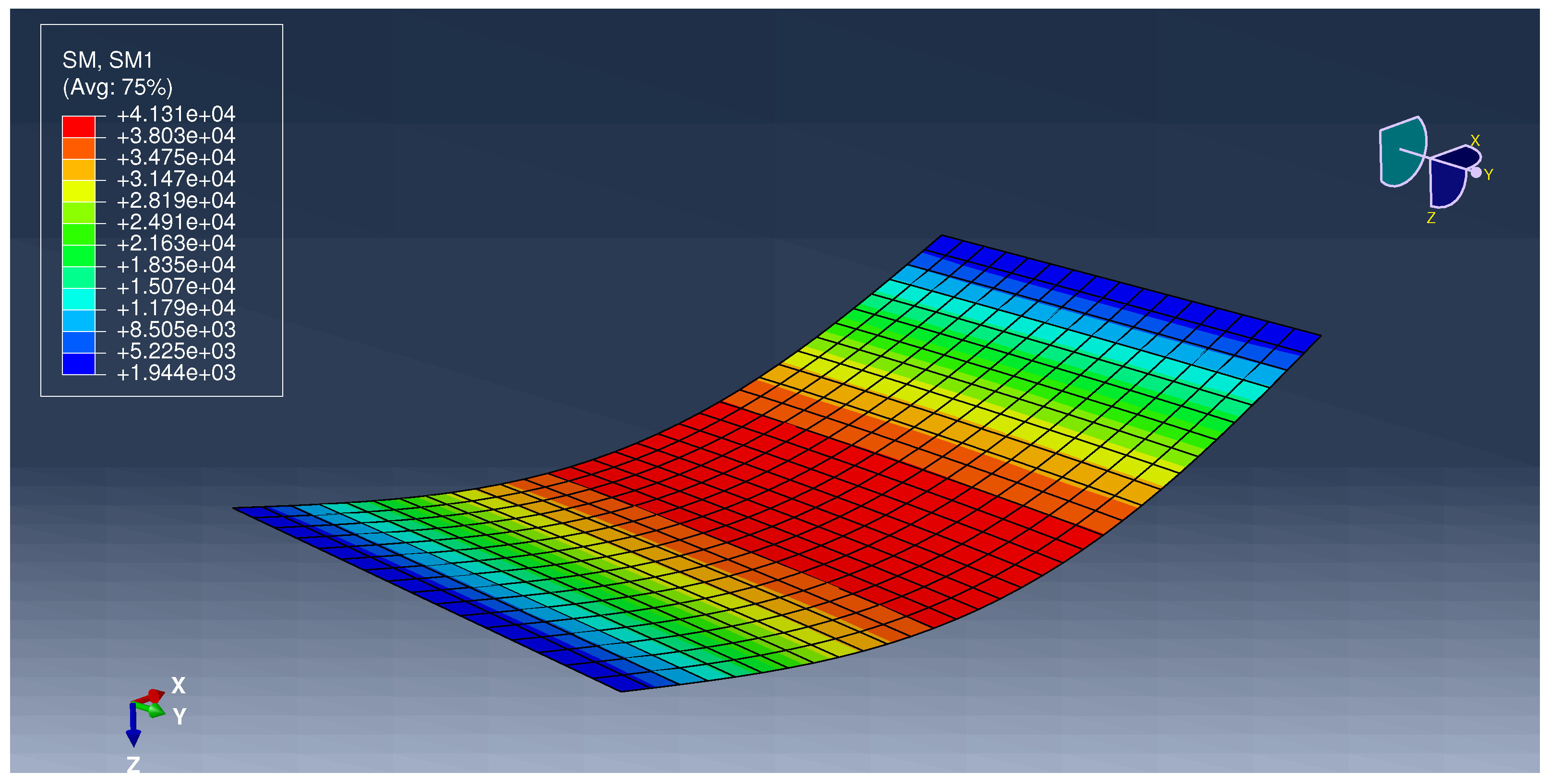
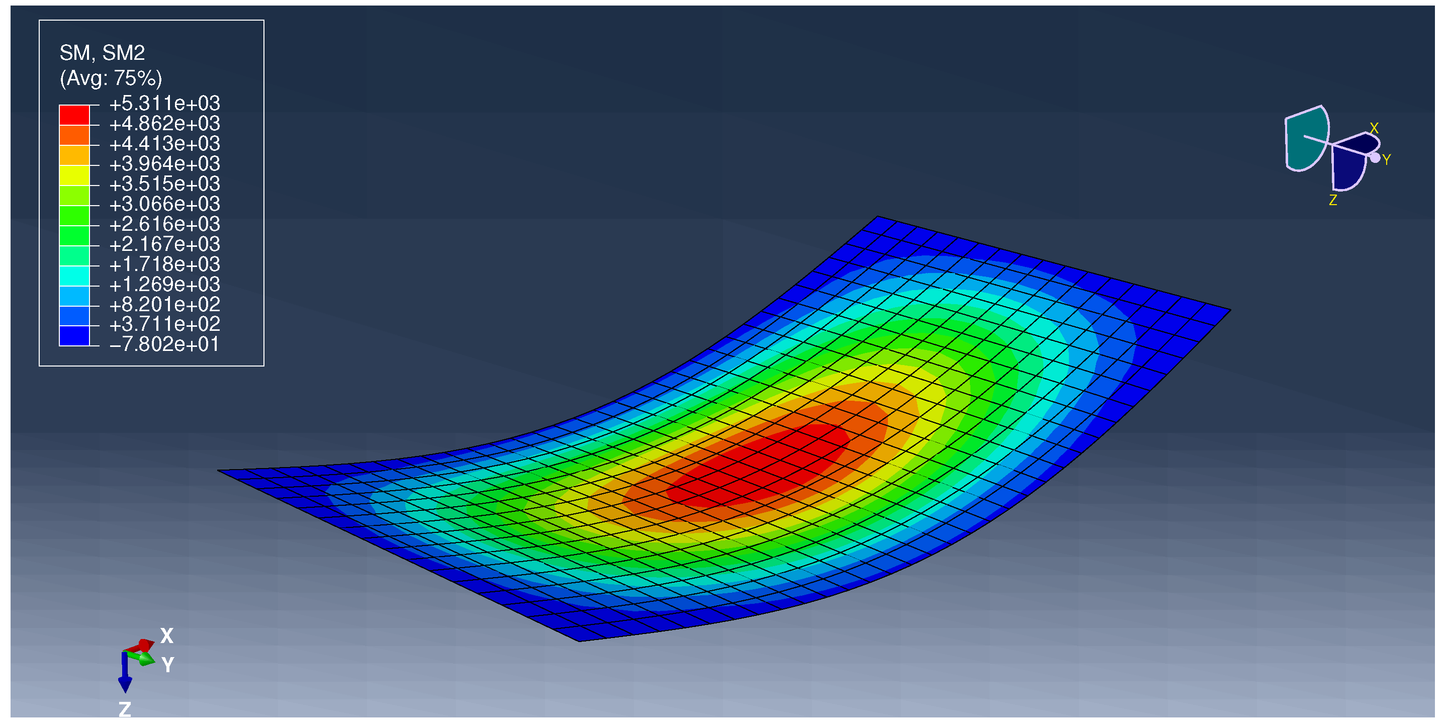
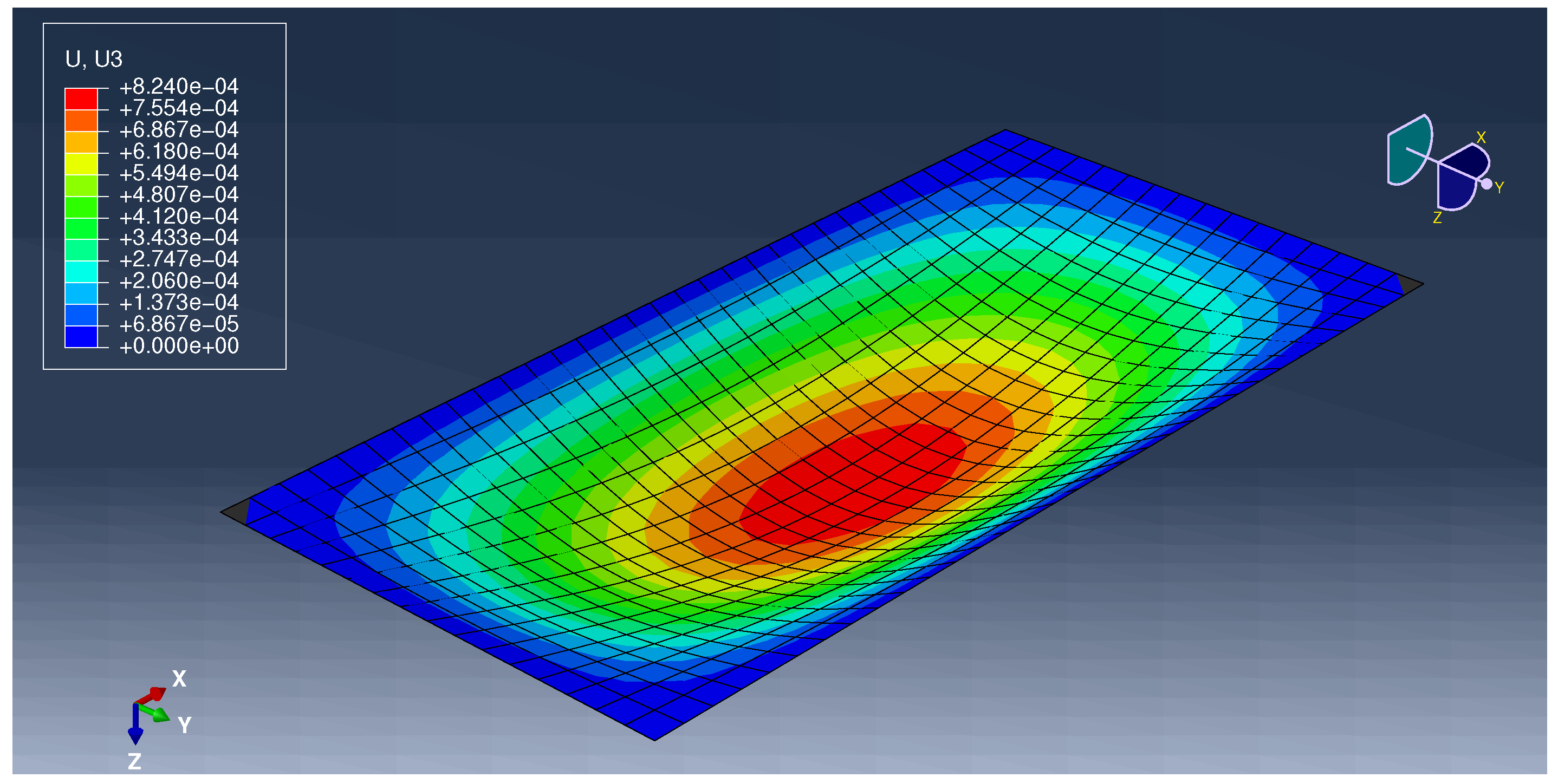
Appendix A. Results from ABAQUS
- 1
- Rectangular plate with two opposite edges simply supported and the other free,
- 2
- Rectangular plate simply supported at the contour,
- 3
- Rectangular plate clamped at the contour.
Appendix A.1. Example 1
Appendix A.2. Example 2
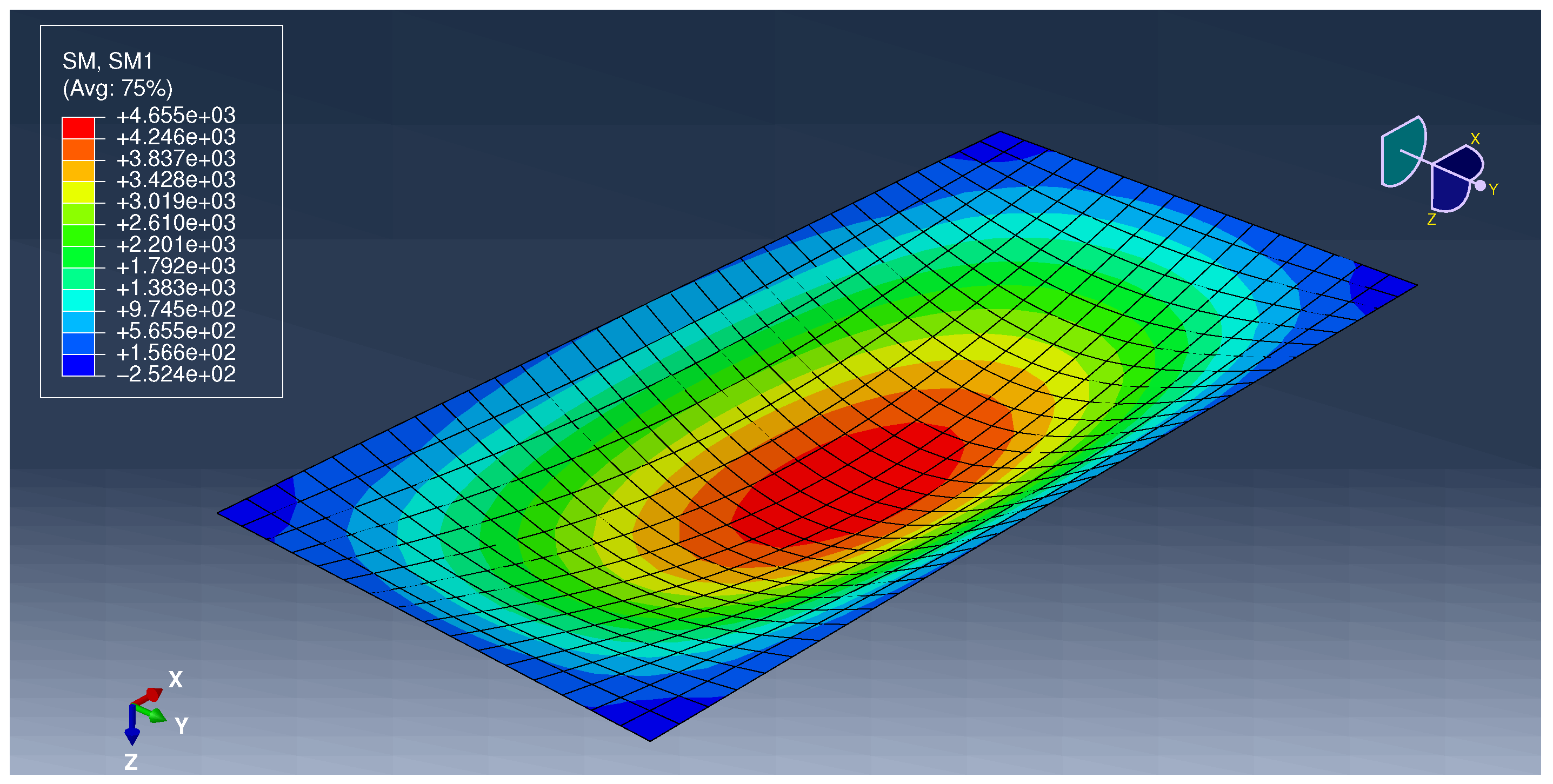
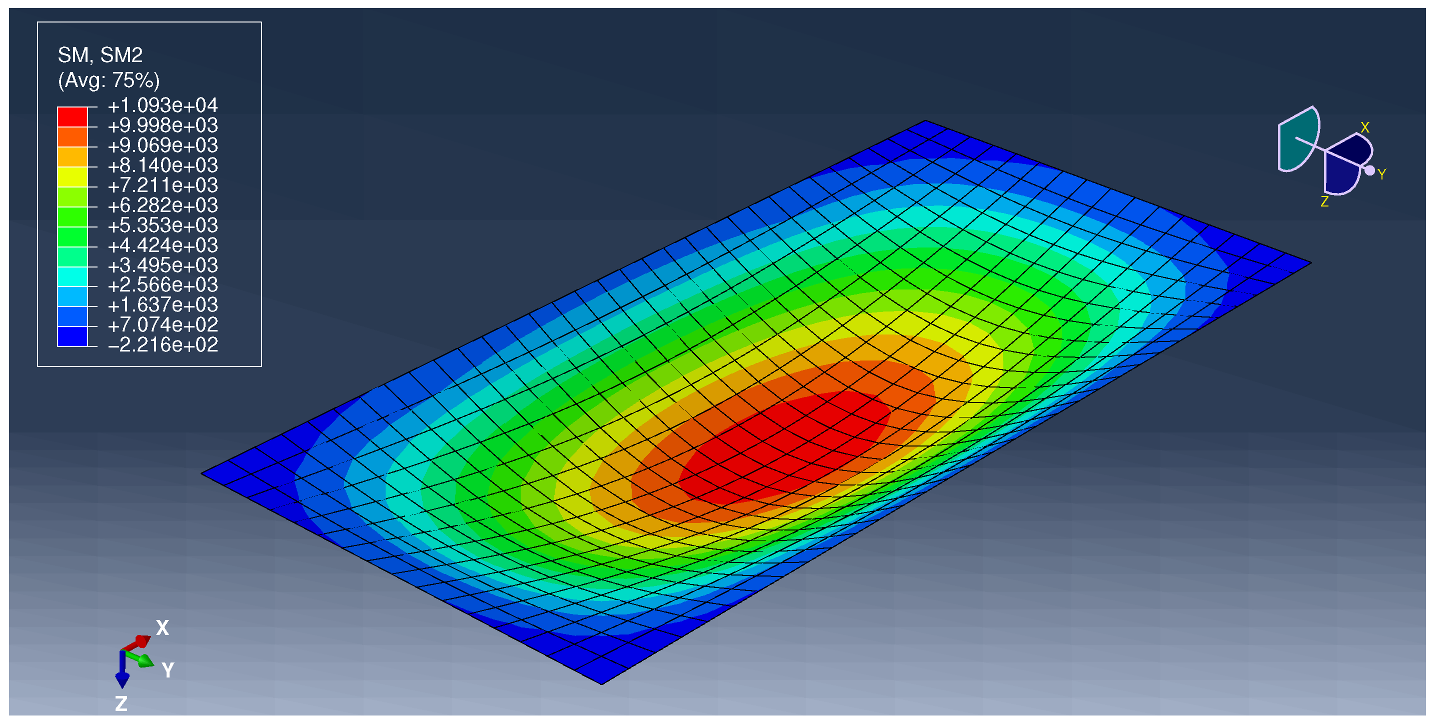
Appendix A.3. Example 3
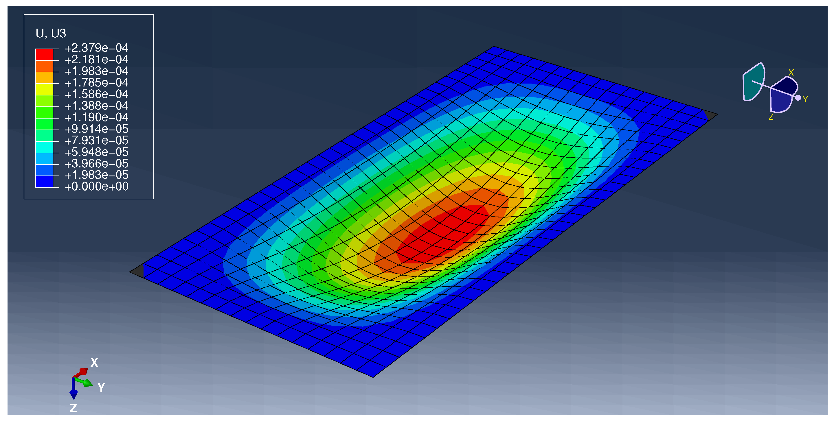

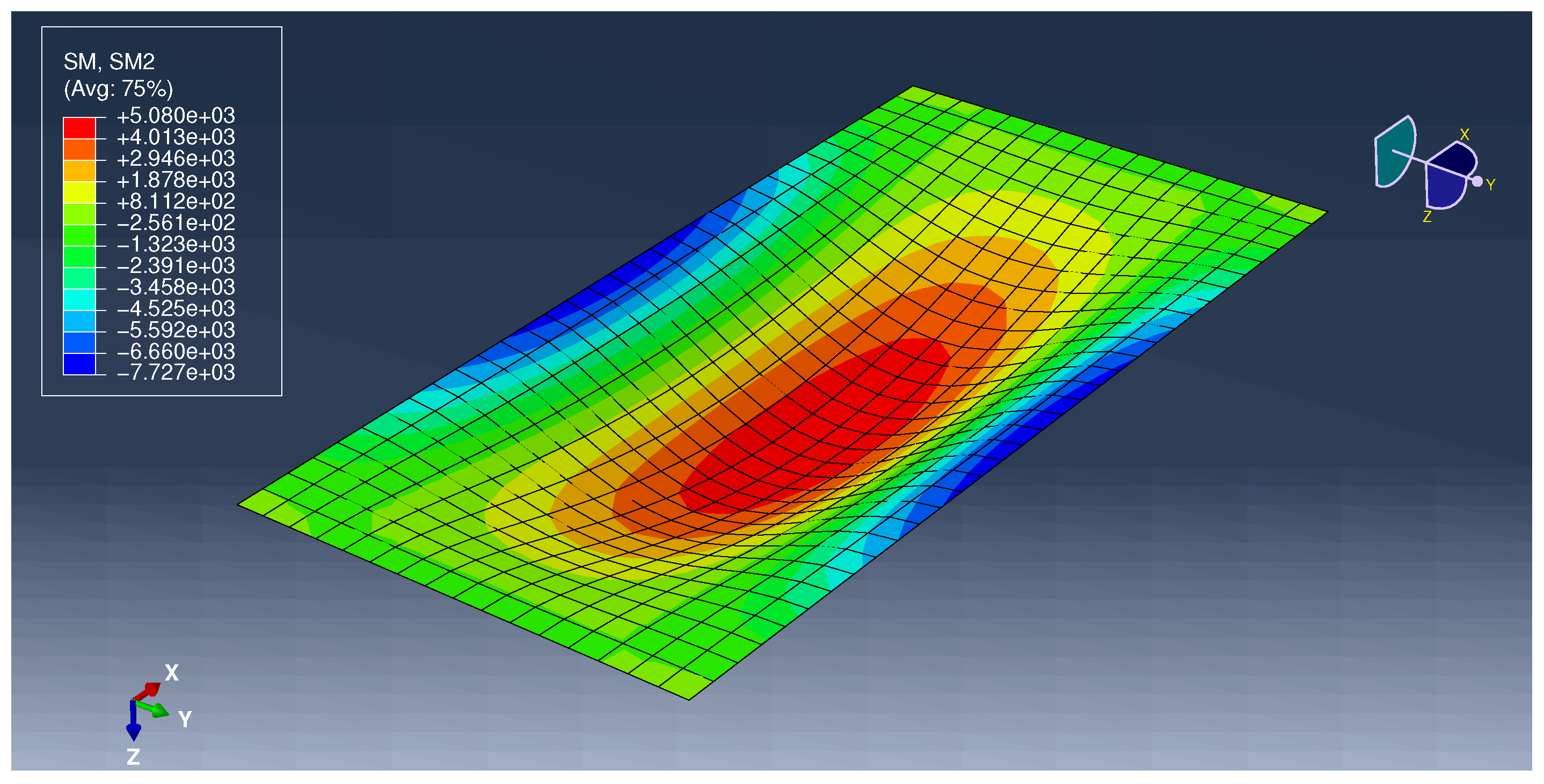
Appendix B. Listing from Author’S Program
import autograd.numpy as np
from autograd import elementwise_grad as grad
import matplotlib.pyplot as plt
from matplotlib import cm
from matplotlib.ticker import LinearLocator
from mpl_toolkits.mplot3d import Axes3D
# ==========
# Parameters
# ==========
# Number of approximations of the solution
_K = 5
# Dimensions
a_1 = 4.  # m
a_2 = 2.  # m
h = 0.2   # m
# Young’s modulus
E = 3e10  # Pa
# Poisson ratio
nu = 0.2
# Intensity of the load
q_0 = 10_000.00  # N
# Flexural rigidity of a plate
D = (E * h**3) / (12*(1-nu**2))
# ================
# Helper functions
# ================
def a(s):
    if s == 1:
        return a_1
    elif s == 2:
        return a_2
def x(s):
    def wrapper(x_1, x_2):
        if s == 1:
            return x_1
        elif s == 2:
            return x_2
    return wrapper
def gamma(k, s):
    return (k*np.pi) / a(s)
def delta(k, s):
    return ((2*k-1)*np.pi) / (2*a(s))
def kappa(k, p, s):
    if p == 1:
        return gamma(k, s)
    elif p == 2:
        return delta(k, s)
def T(k, p, s):
    def wrapper(x_1, x_2):
        return np.cos(kappa(k, p, s) * x(s)(x_1, x_2))
    return wrapper
def calculate(fs, solution, x_1, x_2):
    coeffs = np.array([f(x_1, x_2) for f in fs])
    return np.einsum(’ijk,i->jk’, coeffs, solution)
def particular_solution(C, f):
    def wrapper(x_1, x_2):
        return C * f(x_1, x_2)
    return wrapper
def final(general_solution, particular_solution):
    result = []
    for f in general_solution:
        result.append(f)
    result.append(particular_solution)
    return result
# ====================================================
# Relations known from theory of thin isotropic plates
# ====================================================
def phi_1(w):
    def wrapper(x_1, x_2):
        return grad(w, 0)(x_1, x_2)
    return wrapper
def phi_2(w):
    def wrapper(x_1, x_2):
        return grad(w, 1)(x_1, x_2)
    return wrapper
def M_11(w):
    def wrapper(x_1, x_2):
        return -D * (grad(grad(w, 0), 0)(x_1, x_2) +
               nu*grad(grad(w, 1), 1)(x_1, x_2))
    return wrapper
def M_22(w):
    def wrapper(x_1, x_2):
        return -D * (grad(grad(w, 1), 1)(x_1, x_2) +
                     nu*grad(grad(w, 0), 0)(x_1, x_2))
    return wrapper
def M_12(w):
    def wrapper(x_1, x_2):
        return -D * (1-nu) * grad(grad(w, 0), 1)(x_1, x_2)
    return wrapper
def Q_1(w):
    def wrapper(x_1, x_2):
        return -D * (grad(grad(grad(w, 0), 0), 0)(x_1, x_2) +
               grad(grad(grad(w, 0), 1), 1)(x_1, x_2))
    return wrapper
def Q_2(w):
    def wrapper(x_1, x_2):
        return -D * (grad(grad(grad(w, 0), 0), 1)(x_1, x_2) +
               grad(grad(grad(w, 1), 1), 1)(x_1, x_2))
    return wrapper
def V_1(w):
    def wrapper(x_1, x_2):
        return -D * (grad(grad(grad(w, 0), 0), 0)(x_1, x_2) +
               (2-nu)*grad(grad(grad(w, 0), 1), 1)(x_1, x_2))
    return wrapper
def V_2(w):
    def wrapper(x_1, x_2):
        return -D * (grad(grad(grad(w, 1), 1), 1)(x_1, x_2) +
               (2-nu)*grad(grad(grad(w, 0), 0), 1)(x_1, x_2))
    return wrapper
# ===============
# Force functions
# ===============
def force_functions(m, n, p, q):
    def wrapper(x_1, x_2):
        return T(m, p, 1)(x_1, x_2) * T(n, q, 2)(x_1, x_2)
    return wrapper
# ===============
# Shape functions
# ===============
# Base functions of the solution
def B(k, p, s, ni):
    def wrapper(x_1, x_2):
        if ni == 1:
            return (np.cosh(kappa(k, p, 3-s) * x(s)(x_1, x_2)))
        elif ni == 2:
            return ((x(s)(x_1, x_2) / a(s)) *
                 (np.sinh(kappa(k, p, 3-s) * x(s)(x_1, x_2))))
    return wrapper
# Shape functions
def W(k, p, s, ni):
    def wrapper(x_1, x_2):
        return B(k, p, s, ni)(x_1, x_2) * T(k, p, 3-s)(x_1, x_2)
    return wrapper
def shape_functions(K):
    result = []
    for k in range(1, K+1):
        for p in range(1, 3):
            for s in range(1, 3):
                for ni in range(1, 3):
                    result.append(W(k, p, s, ni))
    return result
# ===========
# Build model
# ===========
W_g = shape_functions(_K)
W_p = force_functions(1, 1, 2, 2)
# ================
# General solution
# ================
# Calculate derivatives of shape function
U_g = [phi_1(f) for f in W_g]
V_g = [phi_2(f) for f in W_g]
X_g = [M_11(f) for f in W_g]
Y_g = [M_22(f) for f in W_g]
Z_g = [M_12(f) for f in W_g]
H_g = [Q_1(f) for f in W_g]
G_g = [Q_2(f) for f in W_g]
K_g = [V_1(f) for f in W_g]
L_g = [V_2(f) for f in W_g]
# ===================
# Particular solution
# ===================
# Calculate derivatives of force function
U_p = phi_1(W_p)
V_p = phi_2(W_p)
X_p = M_11(W_p)
Y_p = M_22(W_p)
Z_p = M_12(W_p)
H_p = Q_1(W_p)
G_p = Q_2(W_p)
K_p = V_1(W_p)
L_p = V_2(W_p)
C = q_0 / (D*(delta(1, 1)**2 + delta(1, 2)**2)**2)
W_s = particular_solution(C, W_p)
U_s = particular_solution(C, U_p)
V_s = particular_solution(C, V_p)
X_s = particular_solution(C, X_p)
Y_s = particular_solution(C, Y_p)
Z_s = particular_solution(C, Z_p)
H_s = particular_solution(C, H_p)
G_s = particular_solution(C, G_p)
K_s = particular_solution(C, K_p)
L_s = particular_solution(C, L_p)
# ==============
# Final solution
# ==============
W = final(W_g, W_s)
U = final(U_g, U_s)
V = final(V_g, V_s)
X = final(X_g, X_s)
Y = final(Y_g, Y_s)
Z = final(Z_g, Z_s)
H = final(H_g, H_s)
G = final(G_g, G_s)
K = final(K_g, K_s)
L = final(L_g, L_s)
# ===================
# Boundary conditions
# ===================
# Initial points
p_1 = np.linspace(0, a_1, 2*_K)
p_2 = np.linspace(0, a_2, 2*_K)
# Boundary points
b_11 = np.full_like(p_2, a_1)
b_12 = p_2
b_21 = p_1
b_22 = np.full_like(p_1, a_2)
# Shape of blocks
m = len(W)
n = 2*_K
# Initialize matrix blocks
B_1 = np.zeros((m, n))
B_2 = np.zeros((m, n))
B_3 = np.zeros((m, n))
B_4 = np.zeros((m, n))
# Fill matrix blocks with values for boundary conditions
for i in range(m):
    B_1[i] = W[i](b_11, b_12)
    B_2[i] = U[i](b_11, b_12)
    B_3[i] = W[i](b_21, b_22)
    B_4[i] = V[i](b_21, b_22)
# ============
# Solve system
# ============
# Augmented matrix
M = np.hstack((B_1, B_2, B_3, B_4))
M = M.T
# Coefficient matrix
A = M[:, :-1]
# Column vector of constant terms
b = M[:, -1]
# Solve a linear matrix equation
R = np.linalg.solve(A, -b)
R = np.append(R, 1)
# ==========================
# Calculate and plot results
# ==========================
# Prepare points for calculating the values in them
x_1 = np.linspace(-a_1, a_1, num=51)
x_2 = np.linspace(-a_2, a_2, num=51)
X_1, X_2 = np.meshgrid(x_1, x_2)
for f in [W, U, V, X, Y, Z, H, G, K, L]:
    X_3 = calculate(f, R, X_1, X_2)
    fig = plt.figure()
    ax = fig.gca(projection=’3d’)
    ax.set_xlabel(’$x_1$’)
    ax.set_ylabel(’$x_2$’)
    ax.set_zlabel(’$x_3$’)
    surf = ax.plot_surface(X_1, X_2, X_3,
                      cmap=cm.coolwarm,
                      linewidth=0,
                      antialiased=True)
    ax.zaxis.set_major_locator(LinearLocator(10))
    ax.set_zlim(ax.get_zlim()[::-1])
    boundaries = np.linspace(np.min(X_3), np.max(X_3), 25)
    fig.colorbar(surf,
              shrink=0.75,
              aspect=5,
              boundaries=boundaries)
    plt.show()
--------------------------------------------------------------------------------
References
- Reddy, J. Theory of Elastic Plates and Shells, 2nd ed.; CRC Press Taylor & Francis Group: London, UK; New York, NY, USA, 2010. [Google Scholar]
- Szilard, R. Theories and Applications of Plate Analysis. Classical, Numerical and Engineering Methods. Appl. Mech. Rev. 2004, 57, B32–B33. [Google Scholar] [CrossRef]
- Dolbow, J.; Moës, N.; Belytschko, T. Modeling fracture in Mindlin–Reissner plates with the extended finite element method. Int. J. Solids Struct. 2000, 37, 7161–7183. [Google Scholar] [CrossRef]
- Reddy, J. Third-Order Theory of Laminated Composite Plates and Shells. In Mechanics of Laminated Composite Plates and Shells; CRC Press: Boca Raton, IL, USA, 2003; p. 671. [Google Scholar]
- Wang, C.; Reddy, J.; Lee, K. An Overview of Plate Theories. In Shear Deformable Beams and Plates: Relationships with Classical Solutions; Elsevier Science Ltd.: Amsterdam, The Netherlands, 2000; p. 3. [Google Scholar]
- Rakowski, G. Sprężystość. Problemy i RozwiąZania. Metody Analityczne i Numeryczne; Wydawnictwo Politechniki Świętokrzyskiej: Kielce, Poland, 2001. [Google Scholar]
- Timoshenko, S.; Woinowsky-Krieger, S. Simply supported rectangular plates. In Theory of pLates and Shells; McGraw-Hill Book Company, Inc.: New York, NY, USA, 1959; pp. 105–108. [Google Scholar]
- Timoshenko, S.P. Kurs Teorii Uprugosti; Naukova Dumka: Kiev, Ukraine, 1972; pp. 320–364. [Google Scholar]
- Grzymkowski, R.; Kapusta, A.; Nowak, I.; Słota, D. Metody Numeryczne. Zagadnienia Brzegowe; WPKJS: Gliwice, Poland, 2003. [Google Scholar]
- Skibicki, D.; Nowicki, K. Metody Numeryczne w Budowie Maszyn; Wydawnictwa Uczelniane Akademii Techniczno-Rolniczej w Bydgoszczy: Bydgoszcz, Poland, 2006. [Google Scholar]
- Wilson, E. Special numerical and computer techniques for the analysis of finite element systems. In U.S.–Germany Symposium on Finite Elements Methods; MIT: Cambridge, MA, USA, 1976. [Google Scholar]
- Kleiber, M. Mechanika Techniczna. Komputerowe Metody Mechaniki Ciał StałYch; PWN: Warszawa, Poland, 1995. [Google Scholar]
- Qin, Q. The Trefftz Finite and Boundary Element Method; WIT Press: Southampton, Boston, IL, USA, 2000. [Google Scholar]
- Zienkiewicz, O.; Taylor, R. The Finite Element Method, 5th ed.; Butterworth Heinemann: Oxford, UK, 2000; Volume 2. [Google Scholar]
- Sikora, J. Numeryczne Metody Rozwiązywania Zagadnień Brzegowych. Podstawy Metody Elementów Skończonych i Metody Elementów Brzegowych; Politechnika Lubelska: Lublin, Poland, 2011. [Google Scholar]
- Fadhil, S.; El-Zafrany, A. Boundary element analysis of thick Reissner plates on two-parameter foundation. Int. J. Solids Struct. 1994, 31, 2901–2917. [Google Scholar] [CrossRef]
- Brebbia, C. The Boundary Element Method for Engineers; Pentech Press: London, UK, 1978. [Google Scholar]
- Myślecki, K. Metoda Elementów Brzegowych w Statyce Dźwigarów Powierzchniowych; Oficyna Wydawnicza Politechniki Wrocławskiej: Wrocław, Poland, 2004. [Google Scholar]
- Baydin, A.G.; Pearlmutter, B.A.; Radul, A.A. Automatic differentiation in machine learning: A survey. J. Mach. Learn. Res. 2017, 18, 5595–5637. [Google Scholar]
- Bradbury, J.; Frostig, R.; Hawkins, P.; Johnson, M.J.; Leary, C.; Maclaurin, D.; Wanderman-Milne, S. JAX: Composable Transformations of Python+NumPy Programs. 2018. Available online: https://github.com/google/jax (accessed on 25 August 2020).
- Woźniak, C. Mechanika Sprężystych Płyt i Powłok; PWN: Warszawa, Poland, 2001. [Google Scholar]
- Nwoji, C.; Mama, B.; Ike, C.; Onah, H. Galerkin-Vlasov Method for the Flexural Analysis of Rectangular Kirchhoff Plates with Clamped and Simply Supported Edges. Iosr J. Mech. Civ. Eng. 2017, 14, 61–74. [Google Scholar] [CrossRef]
- Reddy, J. Energy Principles and Variational Methods in Applied Mechanics, 3rd ed.; John Wiley & Sons, Inc.: New York, NY, USA, 2017. [Google Scholar]
- Navier, C.L.M.H. Extrait des Recherches Sur La Flexion Des Plans Elastiques; Bulletin des Sciences, par la Société Philomatique: Paris, France, 1823; pp. 92–102. [Google Scholar]
- Lévy, M. Sur l’équilibre élastique d’une plaque rectangulaire. Comptes Rendus L’AcadéMie Des Sci. Paris 1899, 129, 535–539. [Google Scholar]
- Krjukov, N. Raschet kosougol’nyh i trapecoidal’nyh plastin s pomoshh’ju splajn funkcij. Prikl. Meh. 1998, 23, 77–81. [Google Scholar]
- Alberg, D.; Nilson, J.; Ullli, D. Teorija splajnov i ee prilozhenie. 1972. Available online: http://libarch.nmu.org.ua/handle/GenofondUA/81626 (accessed on 25 August 2020).
- Songbai, C.; Lasbeng, W. Collocation method for bending problem of cantilevered plates subjected to unsymmetrical loads. Hunan Univ. Natur. Sci. 1996, 23, 126–128. [Google Scholar]
- Dong, C.; Lo, S.; Cheung, Y.; Lee, K. Anisotropic thin plate bending problems by Trefftz boundary collocation method. Eng. Anal. Bound. Elem. 2004, 28, 1017–1024. [Google Scholar] [CrossRef]
- Reddy, J. An Introduction to the Finite Element Method, 3rd ed.; McGraw-Hill: New York, NY, USA, 2006. [Google Scholar]
- Rakowski, G.; Kasperczyk, Z. Metoda Elementów Skończonych w Mechanice Konstrukcji; Oficyna Wydawnicza Politechniki Warszawskiej: Warszawa, Poland, 2005. [Google Scholar]
- The Finite Element Method: Its Basis and Fundamentals, 7th ed.; Zienkiewicz, O., Taylor, R., Zhu, J., Eds.; Butterworth-Heinemann: Oxford, UK, 2013. [Google Scholar] [CrossRef]
- The Finite Element Method for Solid and Structural Mechanics, 7th ed.; Zienkiewicz, O., Taylor, R., Fox, D., Eds.; Butterworth-Heinemann: Oxford, UK, 2014. [Google Scholar] [CrossRef]
- Bathe, K.J.; Dvorkin, E.N. A four-node plate bending element based on Mindlin/Reissner plate theory and a mixed interpolation. Int. J. Numer. Methods Eng. 1985, 21, 367–383. [Google Scholar] [CrossRef]
- Podhorecki, A. Metoda elementów czasoprzestrzennych w zastosowaniu do rozwiązywania zagadnień początkowo-brzegowych. In Zeszyty Naukowe; Akademia Techniczno-Rolnicza: Bydgoszcz, Poland, 2004; Volume 54. [Google Scholar]
- Zhuang, M.; Miao, C. Analysis for Irregular Thin Plate Bending Problems on Winkler Foundation by Regular Domain Collocation Method. Math. Probl. Eng. 2018, 2018, 7476954. [Google Scholar] [CrossRef]
- Jiang, W.; Bao, G.; Robert, J. Finite element modeling of stiffened and unstiffened orthotropic plates. Comput. Struct. 1997, 63, 105–117. [Google Scholar] [CrossRef]
- Qu, Z.Q. Model Order Reduction Techniques with Applications in Finite Element Analysis; Springer: London, UK, 2004. [Google Scholar]
- Shen, P.; He, P. Bending analysis of rectangular moderately thick plates using spline finite element method. Comput. Struct. 1995, 54, 1023–1029. [Google Scholar] [CrossRef]
- Dieringer, R.; Hebel, J.; Becker, W. The scaled boundary finite element method for plate bending problems. In Proceedings of the 19th International Conference on Computer Methods in Mechanics 2011, Warsaw, Poland, 9–12 May 2011. [Google Scholar]
- Belyaev, V.; Shapeev, V. Solving the biharmonic equation in irregular domains by the least squares collocation method. AIP Conf. Proc. 2018, 2027, 030094. [Google Scholar] [CrossRef]
- Li, R.; Zhong, Y.; Tian, B. On new symplectic superposition method for exact bending solutions of rectangular cantilever thin plates. Mech. Res. Commun. Mech. Res. Commun. 2011, 38, 111–116. [Google Scholar] [CrossRef]
- Alansari, M.; Afzal, M. Regular and Irregular Plate Deflection Analysis using Matrix Method. IOSR J. Mech. Civ. Eng.-(IOSR-JMCE) 2019, 16, 24–40. [Google Scholar] [CrossRef]
- Armando Duarte, C.; Kim, D.J.; Babuška, I. A Global-Local Approach for the Construction of Enrichment Functions for the Generalized FEM and Its Application to Three-Dimensional Cracks. In Advances in Meshfree Techniques; Leitão, V.M.A., Alves, C.J.S., Armando Duarte, C., Eds.; Springer: Dordrecht, The Netherlands, 2007; pp. 1–26. [Google Scholar]
- Duarte, C.; Kim, D.J. Analysis and applications of a generalized finite element method with global–local enrichment functions. Comput. Methods Appl. Mech. Eng. 2008, 197, 487–504. [Google Scholar] [CrossRef]
- Kim, D.J.; Duarte, C.A.; Pereira, J.P. Analysis of Interacting Cracks Using the Generalized Finite Element Method With Global-Local Enrichment Functions. J. Appl. Mech. 2008, 75. [Google Scholar] [CrossRef]
- Gupta, V.; Kim, D.J.; Duarte, C.A. Analysis and improvements of global–local enrichments for the Generalized Finite Element Method. Comput. Methods Appl. Mech. Eng. 2012, 245–246, 47–62. [Google Scholar] [CrossRef]
- Malekan, M.; Barros, F.A.c.B.; Pitangueira, R.L.S.; Alves, P.D. An Object-Oriented Class Organization for Global-Local Generalized Finite Element Method. Lat. Am. J. Solids Struct. 2016, 13, 2529–2551. [Google Scholar] [CrossRef]
- Malekan, M.; Barros, F.; Pitangueira, R.; Alves, P.; Penna, S. A computational framework for a two-scale generalized/extended finite element method: Generic imposition of boundary conditions. Eng. Comput. 2016, 34. [Google Scholar] [CrossRef]
- Malekan, M.; Barros, F.B. Well-conditioning global–local analysis using stable generalized/extended finite element method for linear elastic fracture mechanics. Comput. Mech. 2016, 58, 819–831. [Google Scholar] [CrossRef]
- Malekan, M.; Barros, F.B.; Pitangueira, R.L. Fracture analysis in plane structures with the two-scale G/XFEM method. Int. J. Solids Struct. 2018, 155, 65–80. [Google Scholar] [CrossRef]
- Baiz, P.; Natarajan, S.; Bordas, S.; Kerfriden, P.; Rabczuk, T. Linear buckling analysis of cracked plates by SFEM and XFEM. J. Mech. Mater. Struct. 2011, 6, 1213–1238. [Google Scholar] [CrossRef][Green Version]
- Nasirmanesh, A.; Mohammadi, S. XFEM buckling analysis of cracked composite plates. Compos. Struct. 2015, 131, 333–343. [Google Scholar] [CrossRef]
- Perumal, L.; Tso, C.; Leng, L.T. Analysis of thin plates with holes by using exact geometrical representation within XFEM. J. Adv. Res. 2016, 7, 445–452. [Google Scholar] [CrossRef] [PubMed]
- Benvenuti, E. An effective XFEM with equivalent eigenstrain for stress intensity factors of homogeneous plates. Comput. Methods Appl. Mech. Eng. 2017, 321, 427–454. [Google Scholar] [CrossRef]
- Donning, B.M.; Liu, W.K. Meshless methods for shear-deformable beams and plates. Comput. Methods Appl. Mech. Eng. 1998, 152, 47–71. [Google Scholar] [CrossRef]
- Shao, W.; Wu, X. Chebyshev tau meshless method based on the highest derivative for solving a class of two-dimensional parabolic problems. Wit Trans. Model. Simul. 2013. [Google Scholar] [CrossRef]
- Liu, N.; Jeffers, A.E. A geometrically exact isogeometric Kirchhoff plate: Feature-preserving automatic meshing and C1 rational triangular Bézier spline discretizations. Int. J. Numer. Methods Eng. 2018, 115, 395–409. [Google Scholar] [CrossRef]
- Liu, N.; Ren, X.; Lua, J. An isogeometric continuum shell element for modeling the nonlinear response of functionally graded material structures. Compos. Struct. 2020, 237, 111893. [Google Scholar] [CrossRef]
- Batista, M. Uniformly Loaded Rectangular Thin Plates with Symmetrical Boundary Conditions. arXiv 2010, arXiv:1001.3016. [Google Scholar]
- Batista, M. New analytical solution for bending problem of uniformly loaded rectangular plate supported on corner points. IES J. Part Civ. Struct. Eng. 2010, 3, 75–84. [Google Scholar] [CrossRef]
- Li, R.; Zhong, Y.; Tian, B.; Du, J. Exact bending solutions of orthotropic rectangular cantilever thin plates subjected to arbitrary loads. Int. Appl. Mech. 2011, 47, 107–119. [Google Scholar] [CrossRef][Green Version]
- Ike, C.C. Flexural analysis of rectangular kirchhoff plate on winkler foundation using galerkin-vlasov variational method. Math. Model. Eng. Probl. 2018, 5, 83–92. [Google Scholar] [CrossRef]
- Hwu, C.; Huang, S.T.; Li, C.C. Boundary-based finite element method for two-dimensional anisotropic elastic solids with multiple holes and cracks. Eng. Anal. Bound. Elem. 2017, 79, 13–22. [Google Scholar] [CrossRef]
- Guminiak, M. Zastosowanie metody elementów brzegowych w analizie statyki płyt cienkich. Zesz. Nauk. Politech. Śląskiej 2002, 95, 223–232. [Google Scholar]
- Tanaka, M.; Bercin, A. A boundary element method applied to the elastic bending problem of stiffened plates. Bound. Elem. Method XIX 1997, 19, 203–212. [Google Scholar]
- Delyavskyy, M.; Opanasovych, V.; Bilash, O. Bending by Concentrated Force of a Cantilever Strip Having a Through-thickness Crack Perpendicular to Its Axis. Appl. Sci. 2020, 10, 2037. [Google Scholar] [CrossRef]
- Delyavskyy, M.; Rosiński, K. Analiza statyczna złożonych konstrukcji płytowych w ujęciu makroelementowym. Czas. Inżynierii Lądowej Środowiska i Archit. 2016. [Google Scholar] [CrossRef]
- Delyavskyy, M.; Rosiński, K. Solution of non-rectangular plates with macroelement method. AIP Conf. Proc. 2017, 1822, 020005. [Google Scholar] [CrossRef]
- Delyavs’kyi, M.; Zdolbits’ka, N.; Onyshko, L.; Zdolbits’kyi, A. Determination of the Stress-Strain State in Thin Orthotropic Plates on Winkler’s Elastic Foundations. Mater. Sci. 2015, 50. [Google Scholar] [CrossRef]
- Delyavskyy, M.; Rosiński, K.; Zdolbicka, N.; Bilash, O. Macroelement analysis of thin orthotropic polygonal plate resting on the elastic Winkler’s foundation. AIP Conf. Proc. 2019, 2077, 020014. [Google Scholar] [CrossRef]
- Delyavskyy, M.; Rosiński, K. Analysis of Thin Rectangular Plate Connected With Space Truss; MOSTY Tradycja i Nowoczesność; Wydawnictwa Uczelniane Uniwersytetu Technologiczno-Przyrodniczego w Bydgoszczy: Bydgoszcz, Poland, 2019. [Google Scholar]
- Delyavskyy, M.; Rosiński, K. Rozwiązanie Konstrukcji Inżynierskich w Ujęciu Makroelementowym; Wybrane zagadnienia konstrukcji i materiałów budowlanych oraz geotechniki. Wydawnictwa Uczelniane Uniwersytetu Technologiczno-Przyrodniczego w Bydgoszczy: Bydgoszcz, Poland, 2015. [Google Scholar]
- Barthelemy, J.F.M.; Hall, L.E. Automatic differentiation as a tool in engineering design. Struct. Optim. 1995, 9, 76–82. [Google Scholar] [CrossRef][Green Version]
- Lim, C.W.; Yao, W.A.; Cui, S. Benchmark symplectic solutions for bending of corner-supported rectangular thin plates. IES J. Part Civ. Struct. Eng. 2008, 1, 106–115. [Google Scholar] [CrossRef]
- Li, R.; Wang, B.; Li, G. Benchmark bending solutions of rectangular thin plates point-supported at two adjacent corners. Appl. Math. Lett. 2015, 40, 53–58. [Google Scholar] [CrossRef]
- An, C.; Gu, J.; Su, J. Exact solution of bending problem of clamped orthotropic rectangular thin plates. J. Braz. Soc. Mech. Sci. Eng. 2015, 38. [Google Scholar] [CrossRef]
- Pavlou, D. Main Disadvantages of Finite Element Method. In Essentials of the Finite Element Method For Mechanical and Structural Engineers; Elsevier Inc.: Amsterdam, The Netherlands, 2015. [Google Scholar]

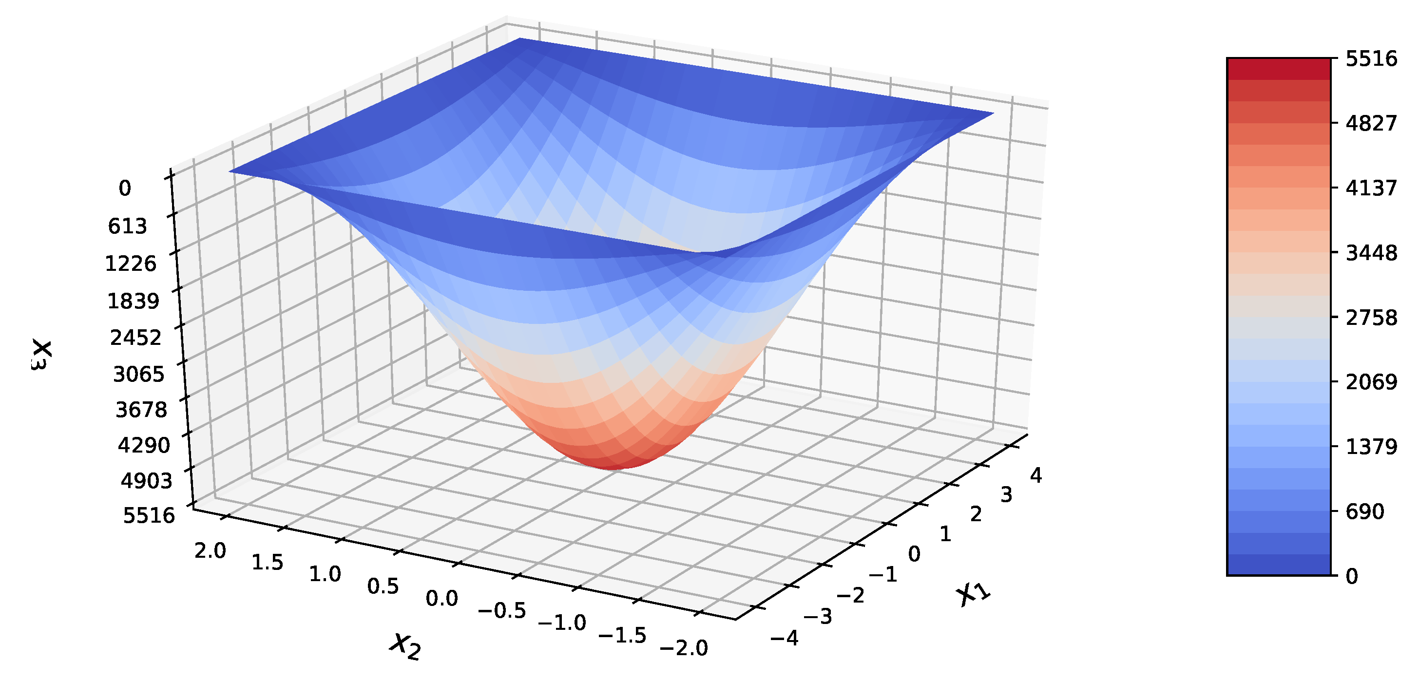
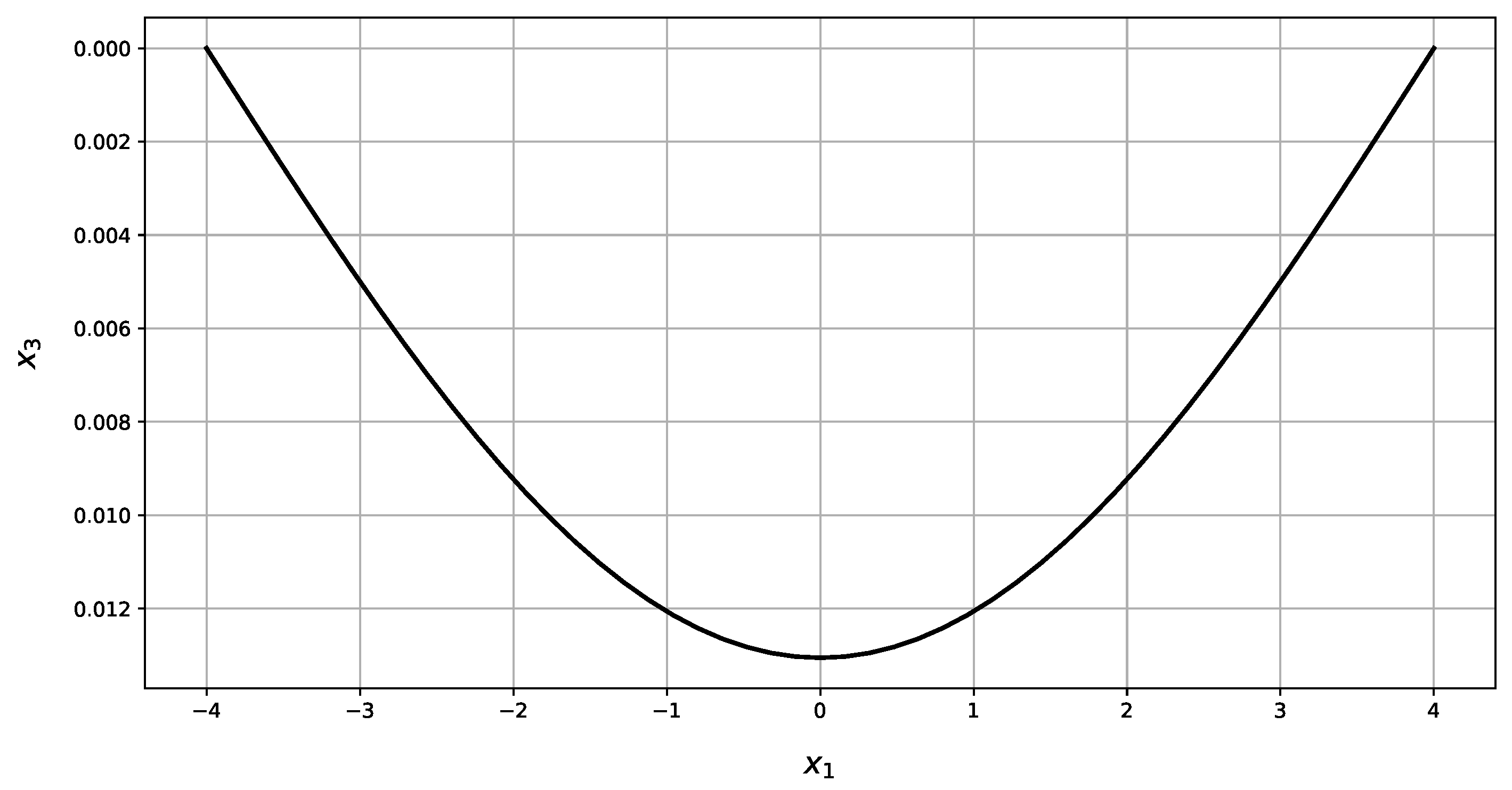
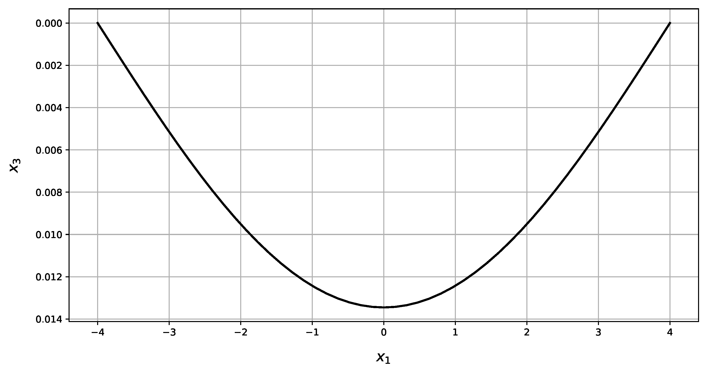
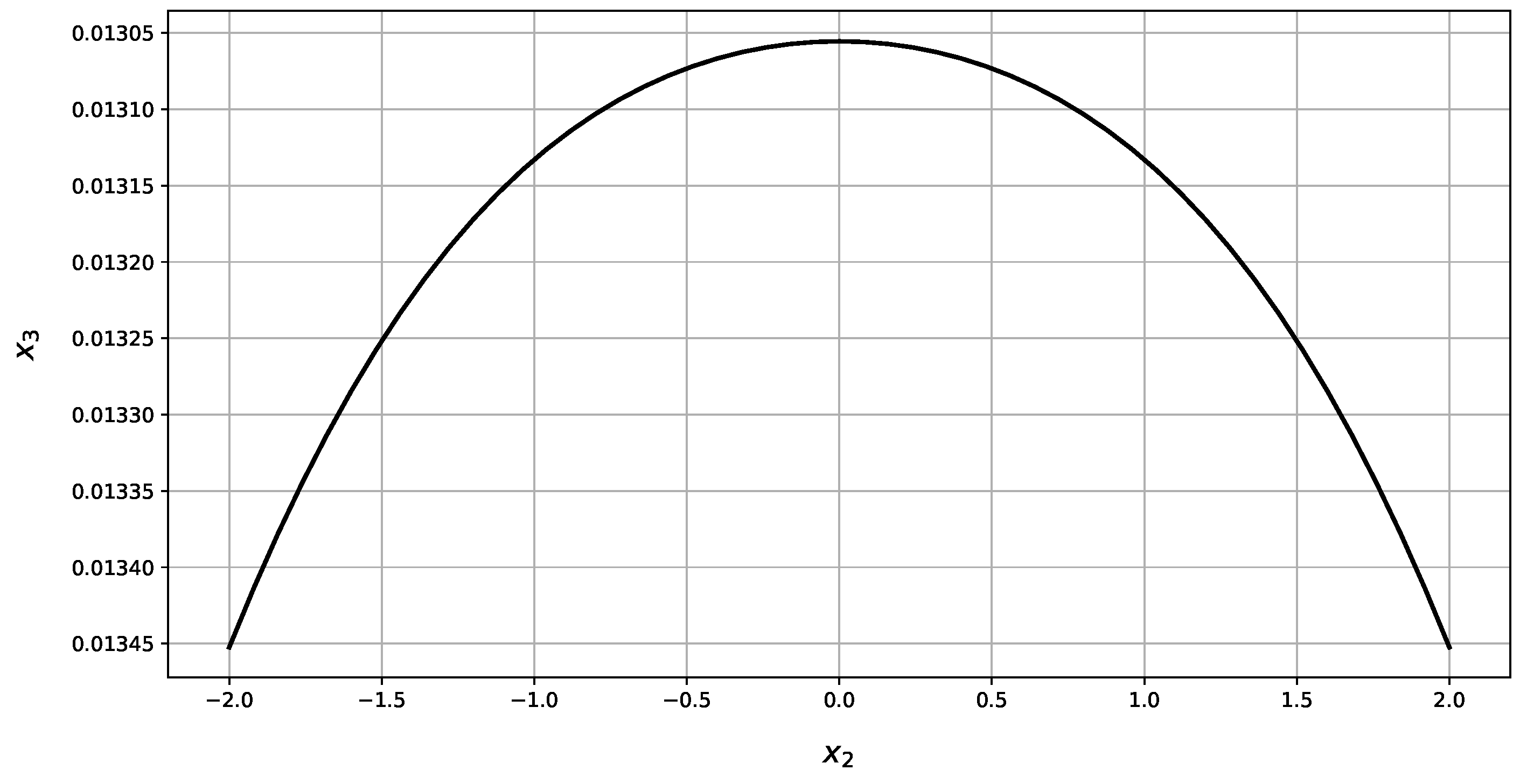
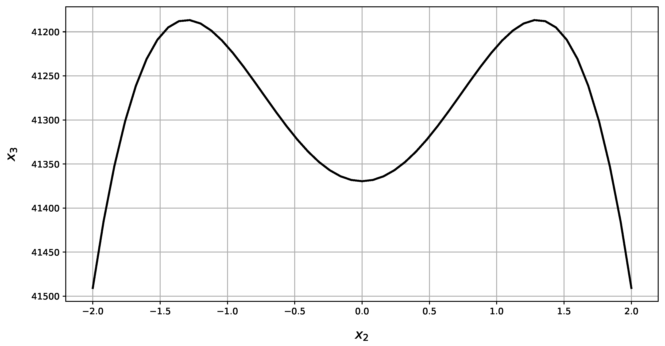
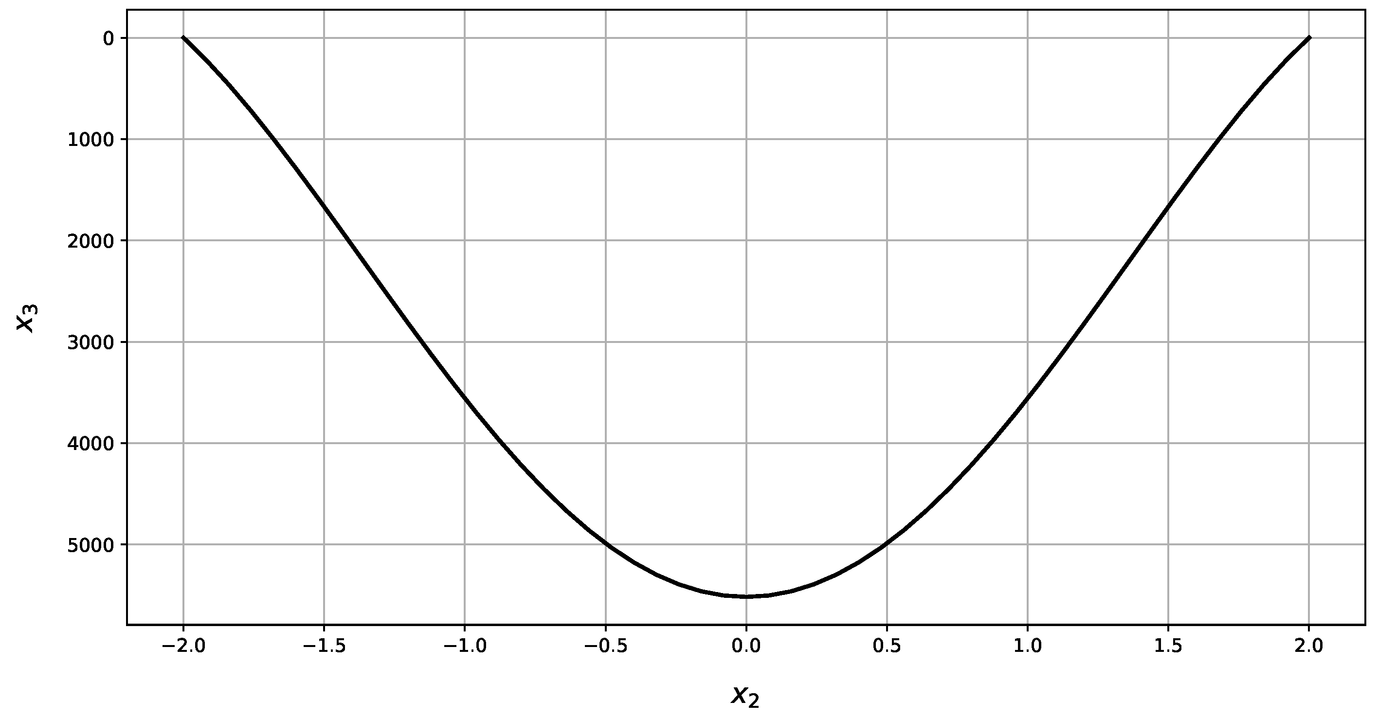
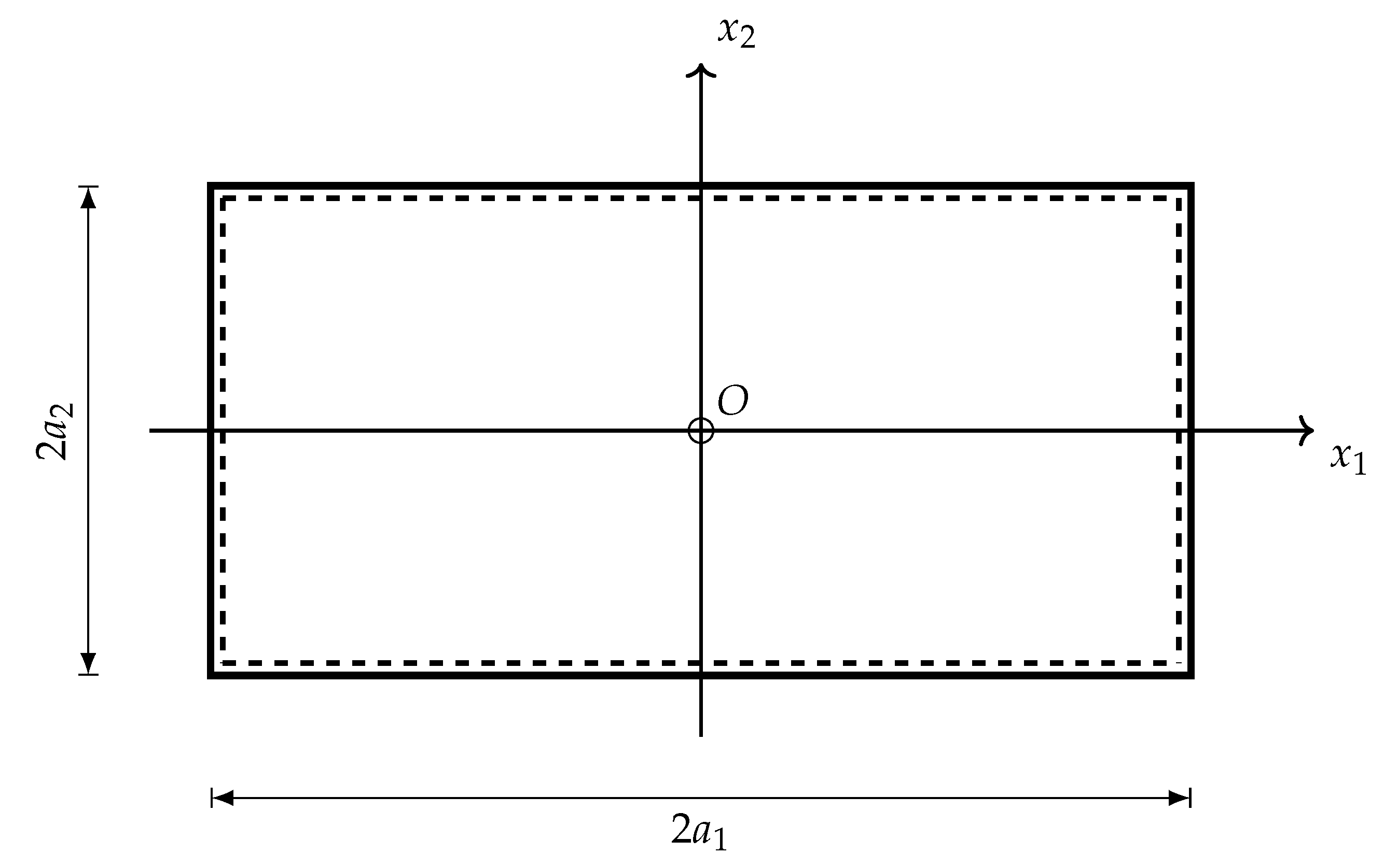
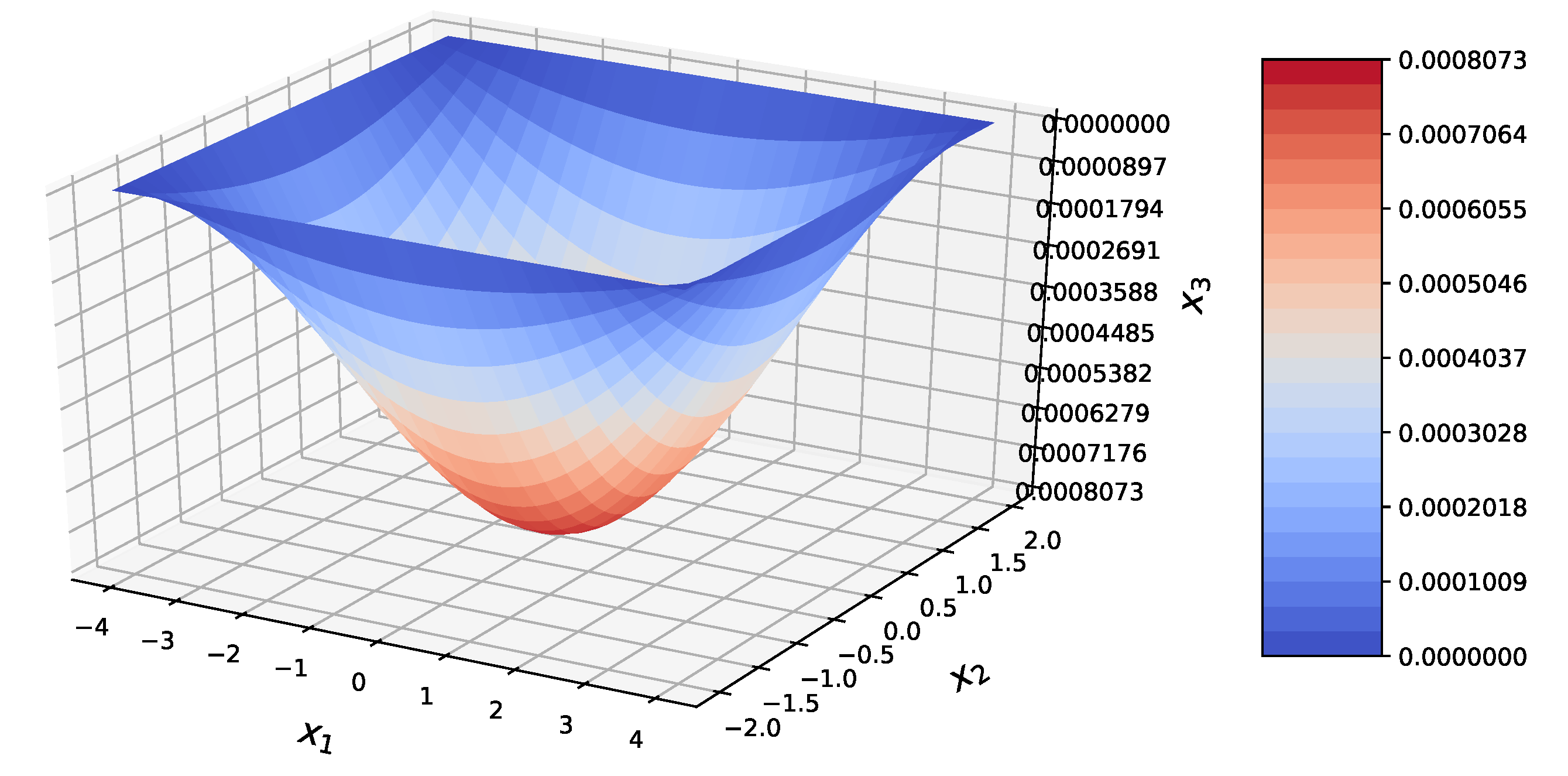
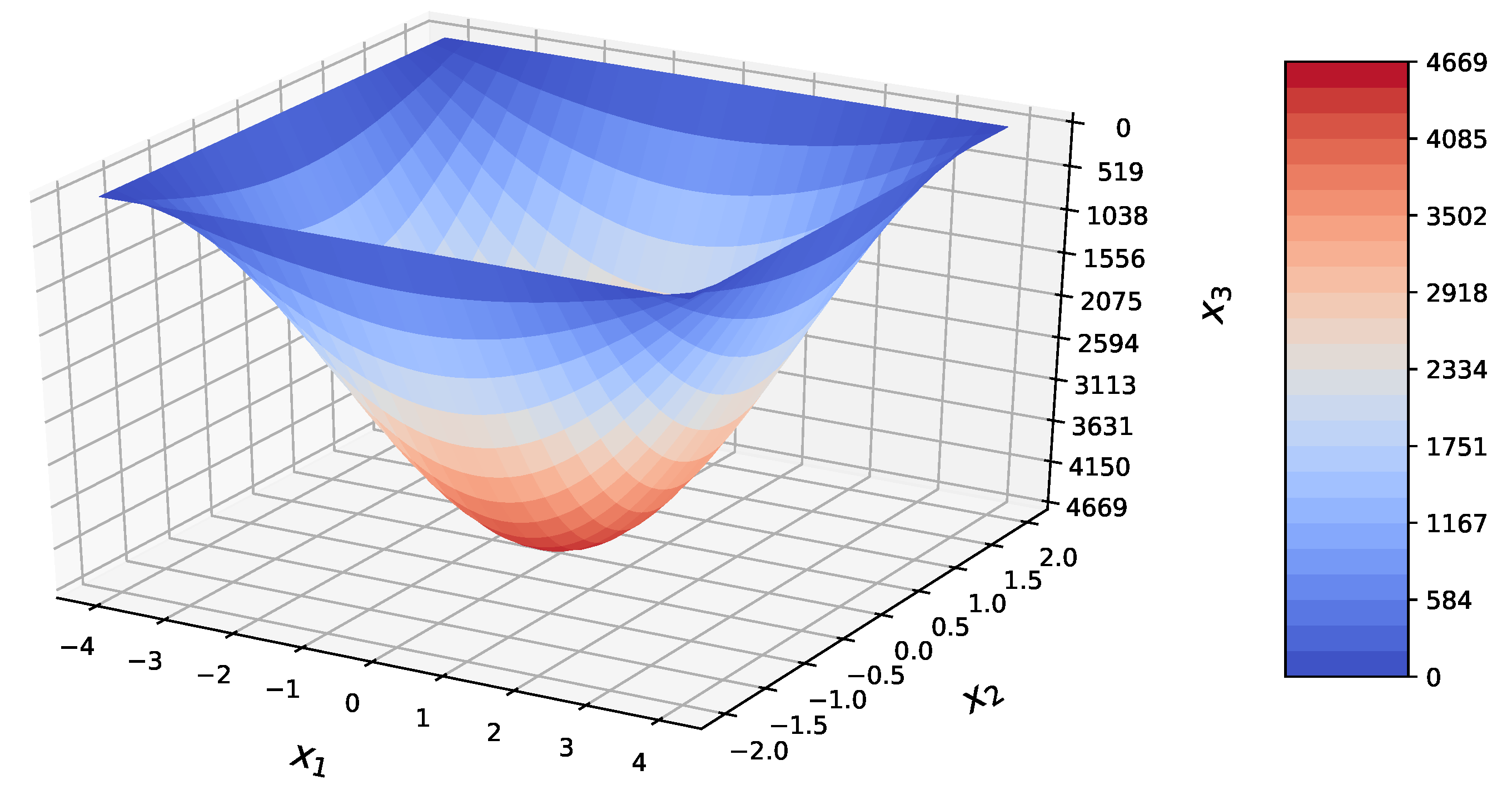
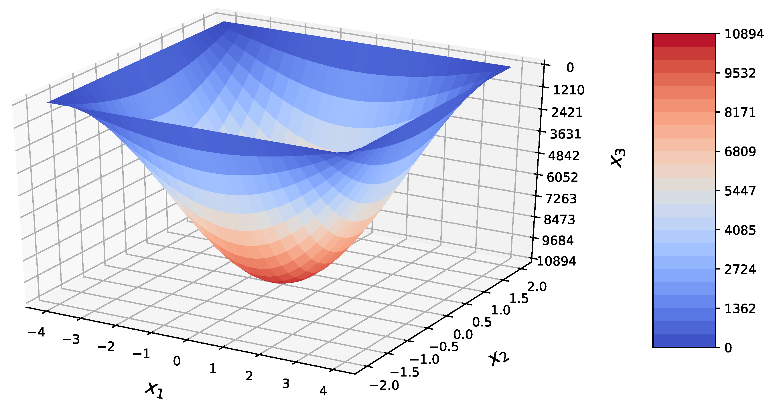
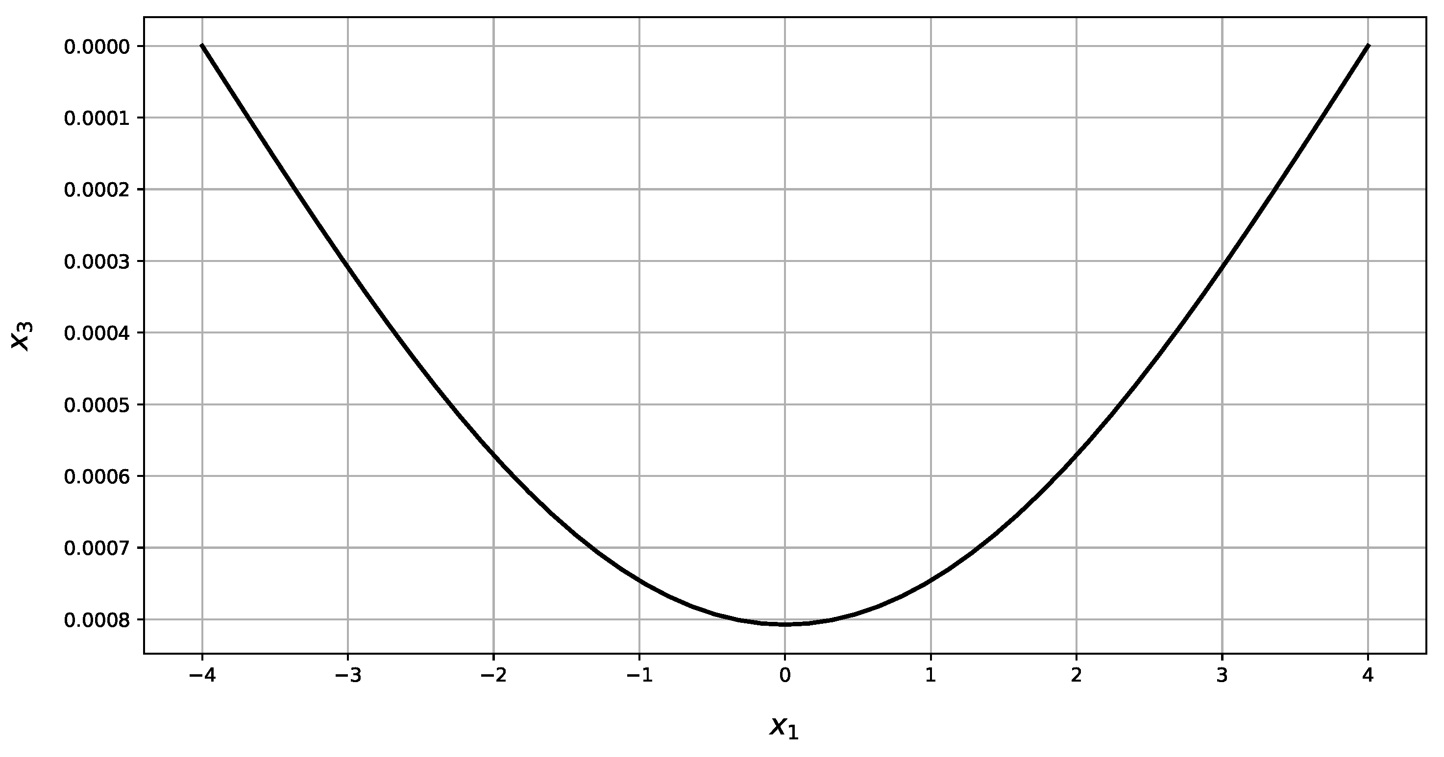
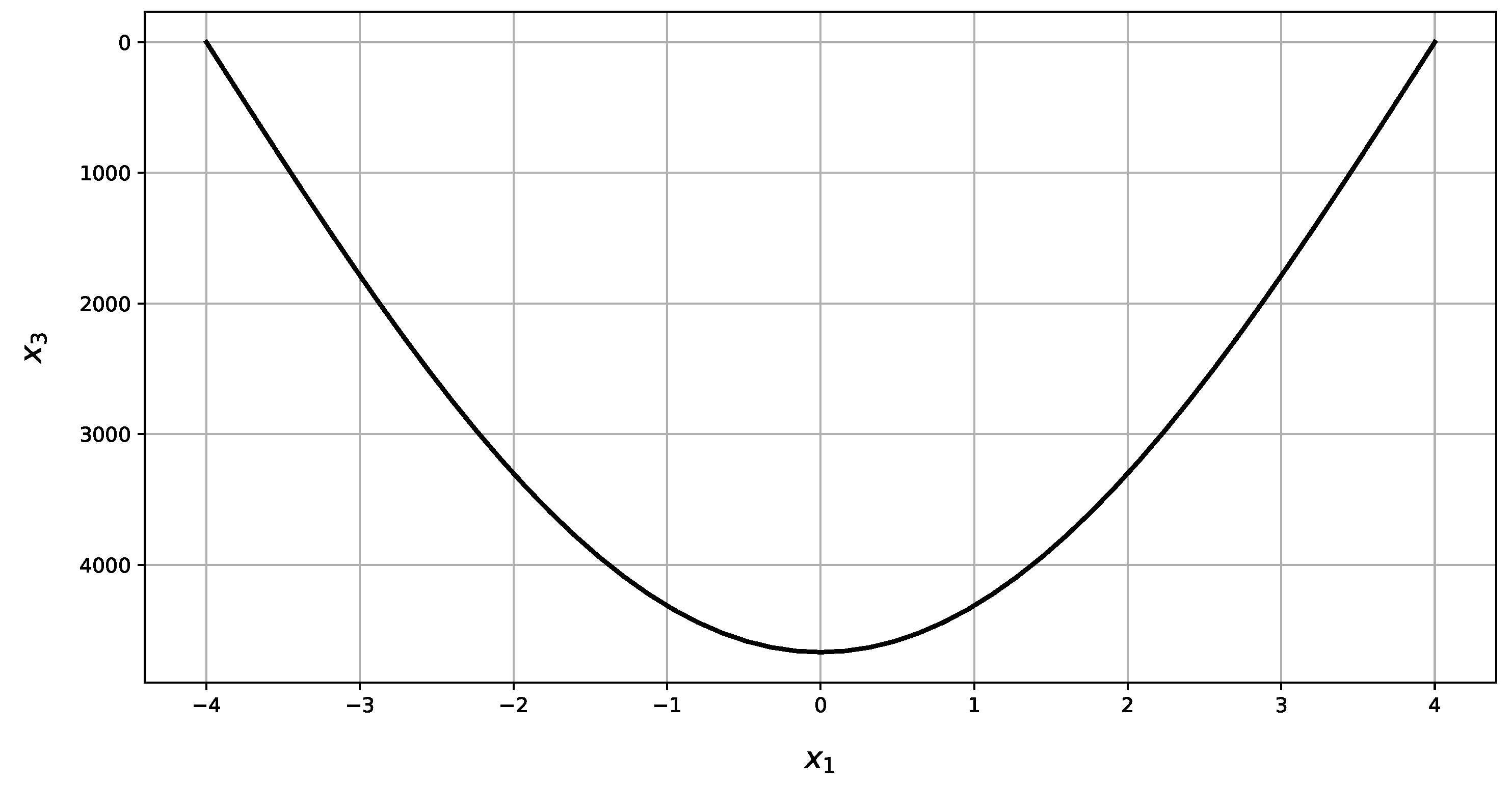



| Present Method | Abaqus | RE | |||||
|---|---|---|---|---|---|---|---|
| Magnitude | Unit | Min | Max | Min | Max | Min | Max |
| w | 0 | 0.013 | 0 | 0.013 | 0% | 0% | |
| 0 | 41,490.63 | 1944 | 41,310 | — | 0.44% | ||
| 0 | 5516.33 | −78.02 | 5311 | — | 3.87% | ||
| −3263.79 | 3263.79 | −2402 | 2402 | 35.88% | 35.88% | ||
| −15,343.36 | 15,343.36 | — | — | — | — | ||
| −3229.42 | 3229.42 | — | — | — | — | ||
| −14,440.95 | 14,440.95 | — | — | — | — | ||
| −2677.45 | 2677.45 | — | — | — | — | ||
| −0.005 | 0.005 | −0.005 | 0.005 | 0% | 0% | ||
| −0.0005 | 0.0005 | −0.0005 | 0.0005 | 0% | 0% | ||
| Magnitude | Edge | Unit | Present Method | Abaqus |
|---|---|---|---|---|
| w | Simply supported | 0 | 0 | |
| Simply supported | 0 | 1966.02 | ||
| Free | 0 | 288.97 | ||
| Free | 0 | — |
| Present Method | Timoshenko | Abaqus | RE | ||||||
|---|---|---|---|---|---|---|---|---|---|
| Magnitude | Unit | Min | Max | Min | Max | Min | Max | Min | Max |
| w | 0.00 | 0.0008 | 0.00 | 0.0008 | 0.00 | 0.0008 | 0% | 0% | |
| 0.00 | 4668.88 | 0.00 | 4668.88 | −252.4 | 4655 | — | 0.30% | ||
| 0.00 | 10,894.05 | 0.00 | 10,894.05 | −221.6 | 10,930 | — | −0.33% | ||
| −4150.12 | 4150.12 | −4150.12 | 4150.12 | −4041 | 4041 | — | 2.70% | ||
| −5092.96 | 5092.96 | −5092.96 | 5092.96 | — | — | — | — | ||
| −10,185.92 | 10,185.92 | −10,185.92 | 10,185.92 | — | — | — | — | ||
| −8352.45 | 8352.45 | −8352.45 | 8352.45 | — | — | — | — | ||
| −11,815.66 | 11,815.66 | −11,815.66 | 11,815.66 | — | — | — | — | ||
| −0.0003 | 0.0003 | −0.0003 | 0.0003 | −0.0003 | 0.0003 | 0% | 0% | ||
| −0.0006 | 0.0006 | −0.0006 | 0.0006 | −0.0006 | 0.0006 | 0% | 0% | ||
| Magnitude | Edge | Unit | Present Method | Timoshenko | Abaqus |
|---|---|---|---|---|---|
| w | Simply supported 1 | 0 | 0 | 0 | |
| Simply supported 1 | 0 | 0 | 416.46 | ||
| w | Simply supported 2 | 0 | 0 | 0 | |
| Simply supported 2 | 0 | 0 | 1170.5 |
| Present Method | Abaqus | RE | |||||
|---|---|---|---|---|---|---|---|
| Magnitude | Unit | Min | Max | Min | Max | Min | Max |
| w | 0.00 | 0.0002 | 0.00 | 0.0002 | 0% | 0% | |
| −4174.73 | 1909.82 | −3326 | 1877 | 25.52% | 1.75% | ||
| −9305.64 | 5180.73 | −7727 | 5080 | 20.43% | 1.98% | ||
| −1190.87 | 1190.87 | −1120 | 1120 | 6.33% | 6.33% | ||
| −6806.21 | 6806.21 | — | — | — | — | ||
| — | — | — | — | ||||
| −7268.18 | 7268.18 | — | — | — | — | ||
| — | — | — | — | ||||
| 0.00 | 0.00 | 0.00 | 0.00 | 0% | 0% | ||
| −0.0002 | 0.0002 | −0.0002 | 0.0002 | 0% | 0% | ||
| Magnitude | Edge | Unit | Present Method | Abaqus |
|---|---|---|---|---|
| w | Clamped 1 | 0 | 0 | |
| Clamped 1 | 0 | 0 | ||
| w | Clamped 2 | 0 | 0 | |
| Clamped 2 | 0 | 0 |
© 2020 by the authors. Licensee MDPI, Basel, Switzerland. This article is an open access article distributed under the terms and conditions of the Creative Commons Attribution (CC BY) license (http://creativecommons.org/licenses/by/4.0/).
Share and Cite
Delyavskyy, M.; Rosiński, K. The New Approach to Analysis of Thin Isotropic Symmetrical Plates. Appl. Sci. 2020, 10, 5931. https://doi.org/10.3390/app10175931
Delyavskyy M, Rosiński K. The New Approach to Analysis of Thin Isotropic Symmetrical Plates. Applied Sciences. 2020; 10(17):5931. https://doi.org/10.3390/app10175931
Chicago/Turabian StyleDelyavskyy, Mykhaylo, and Krystian Rosiński. 2020. "The New Approach to Analysis of Thin Isotropic Symmetrical Plates" Applied Sciences 10, no. 17: 5931. https://doi.org/10.3390/app10175931
APA StyleDelyavskyy, M., & Rosiński, K. (2020). The New Approach to Analysis of Thin Isotropic Symmetrical Plates. Applied Sciences, 10(17), 5931. https://doi.org/10.3390/app10175931


