Neighborhood Aggregation Collaborative Filtering Based on Knowledge Graph

Abstract

In recent years, the research of combining a knowledge graph with recommendation systems has caused widespread concern. By studying the interconnections in knowledge graphs, potential connections between users and items can be discovered, which provides abundant and complementary information for recommendation of items. However, most existing studies have not effectively established the relation between entities and users. Therefore, the recommendation results may be affected by some unrelated entities. In this paper, we propose a neighborhood aggregation collaborative filtering (NACF) based on knowledge graph. It uses the knowledge graph to spread and extract the user’s potential interest, and iteratively injects them into the user features with attentional deviation. We conducted a large number of experiments on three public datasets; we verifyied that NACF is ahead of the most advanced models in top-k recommendation and click-through rate (CTR) prediction.

1. Introduction

At present, many online recommendation services, such as e-commerce, advertising and social media, are based on historical interactions (purchases or clicks) to estimate the user’s interest in the items. Collaborative filtering (CF) personalizes recommendations by analyzing users with similar behaviors [1]. For example, Jamali et al. [2] proposed a random walk model combining the trust-based and collaborative filtering approach for recommendation. Liu et al. [3] developed a Bayesian framework for predicting users’ current news interests. Jamali et al. [4] proposed a social network recommendation method based on matrix decomposition. However, traditional collaborative filtering cannot solve the cold start problem effectively. Generally, researchers add some auxiliary information to solve such problems, such as social network [5], item’s attributes [6], images [7] and heterogeneous network [8]. Among the various auxiliary information, the knowledge graph (KG) usually contains more abundant attributes and relationships about items.

The KG is a multi-relational directed graph composed of a large number of entities and relationships [9]. In recent years, researchers have proposed a number of public KGs (such as Freebase, DBpedia) and commercial KGs (such as the Google Knowledge Graph and Microsoft Satori). These KGs have been successfully applied to KG completion [10], data mining [11], question answering [12], text categorization [13] and many other fields.

At the same time, the combined research of KG and recommendation systems has received more and more attention [14]. As shown in Figure 1, the KG for movie scenario contains more comprehensive ancillary data, such as the background knowledge of the item and the relations between them. This approach can connect the interactions between items in multiple ways and display their potential relationships. More importantly, with rich links of items in KG, we can explore the interests of users in depth to discover their potential interests and complement the interaction of users and items.

It is the key that effectively extracts the auxiliary information in the KG into the recommendation. Recently, some works applied the graph convolutional neural network (GCN) to the recommendation system [15,16,17,18]. However, most of them are designed for user-item interaction graphs or user-item similarities graphs. There are some combined with KG, such as KGCN [18]. However, KGCN only extracts the information of items in the knowledge graph for recommendation, while ignoring the user–item interactions and personalized preferences.

In this work, we proposed neighborhood aggregation collaborative filtering (NACF) based on knowledge graph. The NACF applies GCN to KG to capture the potential relations between users and items and the users’ personalized preferences. Specifically, we embed the user as a new entity type into KG. Their neighbors are items that the they have interacted with. The high-order neighborhood information of user is aggregated in a biased manner when evaluating the interest of a particular user-item pair. The advantages of this method are obvious. On the one hand, the users’ potential interests can be discovered through the proliferation of neighboring entities. On the other hand, we use the attention mechanism to obtain the biased score of the neighboring entities under different user-item pairs, which satisfies individuation in the aggregation.

In summary, the main contributions of this paper are as follows:

• We propose a new neighborhood aggregation collaborative filtering based on a knowledge graph, which iteratively encodes the potential information of the knowledge graph into user features.
• We propose an attention mechanism that is adapted to neighborhood aggregation of the knowledge graph. It takes into account the personalized preferences and multiple associations in the information aggregation.
• We conduct a lot of experiments on three public datasets. The results show that NACF is significantly better than the existing methods in top-k recommendation and click-through rate (CTR) prediction. We also verified that NACF can keep firm performance in cold-start scenarios.

2. Related Work

2.1. Recommendation Based on Knowledge Graph

The existing recommendation schemes based on KGs can be divided into three categories.

(1)

Embedding-based method [6,7,19]. It uses knowledge graph embedding (KGE) algorithm [9] to pre-process the recommended entity in the KG and input the embedding vector into a recommendation framework. For example, DKN [19] combines entity embedding and title embedding as different initial features for news recommendation. CKE [7] combines knowledge graph embedding, text and item images into collaborative filter for unified recommendation. SHINE [6] designed a deep auto-encoder for embedding emotional network, social network and personal data network. However, knowledge graph embedding is usually used to extract the language association of each entity in the knowledge graph, and is more suitable for applications such as link prediction rather than the recommendation system.

(2)

Path-based method [20,21,22]. In the knowledge graph of recommendation, various entities form complex connections, and multiple paths between them can be explored. These paths provide additional information for recommendation, especially on the interpretability. For example, PER [20] uses potential features of meta-path in the KG to represent the connectivity between users and items along different relationships. RKGE [21] and KPRN [22] introduce RNN to model multiple links of the user to items in the KG. The path-based approach makes it easy to take advantage of the connective features of KG. But these methods rely on manually set meta-paths and do not solve the cold-start problem very well. This is not conducive to practical application.

(3)

Graph-based method [18,23,24]. Both the graph-based and path-based method are modeled by knowledge graph structure. The difference is that the graph-based method is not limited to the specific connection between entities, but regards KG as a heterogeneous network centered on a specific user or item. This method propagates from the center entity to extract the characteristics of the corresponding entity. RippleNet [23] proposed the idea of user interest diffusion, which spreads the users’ interest characteristics by various entities of recorded interactions. KGCN [18] combines GCN with KG to extract embedded features of recommended item. Our method is also an example based on knowledge graph structure. But unlike the above algorithm, we embed the user into the KG and personalize the aggregation of user’s characteristics.

2.2. Graph Convolutional Network

The graph convolutional network (GCN) is a deep learning method used to extract spatial features of topological graphs [25], which includes the spectral method [26] and non-spectral method [27]. The spectroscopy method defines the convolution calculation in the Fourier domain by calculating the eigen decomposition of the graph Laplacian. But the learning of the convolution kernel depends on the eigen decomposition of graph laplace matrix, which has certain requirements for the structure of graph and cannot be migrated to the model with other structure. The non-spectral method directly defines the convolutional calculation on the graph and takes into account neighbor nodes of different sizes while maintaining local convolution invariance.

Many of the existing recommendation methods import graph convolution network. PinSage [16] is a recommendation framework for advertising and shopping recommendations in social network. This algorithm combines random walks and graph convolution to generate node embedding that encompasses graph structure and node features. NGCF [17] uses the users’ recorded interactions to generate graph and introduces the GCN to extract the potential features of user. KGCN [18] applies the GCN to the knowledge graph to generate the embedded features of the recommended entity.

In our work, we combine the user-item interactions with the corresponding KG, and introduce the idea of non-spectral GCN to dynamically extract the potential interests of the user.

2.3. Attention Mechanism

The brain receives a lot of external information all the time. When the brain receives the information, it will consciously or unconsciously use the attention mechanism to obtain more important information for itself. In recent years, the attention mechanism has been introduced into the fields of natural language processing, object detection, semantic segmentation, etc., and has achieved great effects.

The attention mechanism is also naturally applied to the recommendation system. DKN [19] builds a attention module to calculate the similarity between interactive items and recommended items. RippleNet [23] uses the similarity of the knowledge graph triples to calculate weights for different neighborhood entities. DIN [28] proposes a framework that uses the interest distribution to represent the diverse interest of user, and uses the attention mechanism to dynamically activate users’ interests in different recommended items.

Our work is obviously different from the above. We not only consider the degree of user interest in the propagation of knowledge graph, but also consider the similarity between each entity in user’s neighborhood and current recommended entity.

3. NACF Framework

3.1. Knowledge Graph Introduction

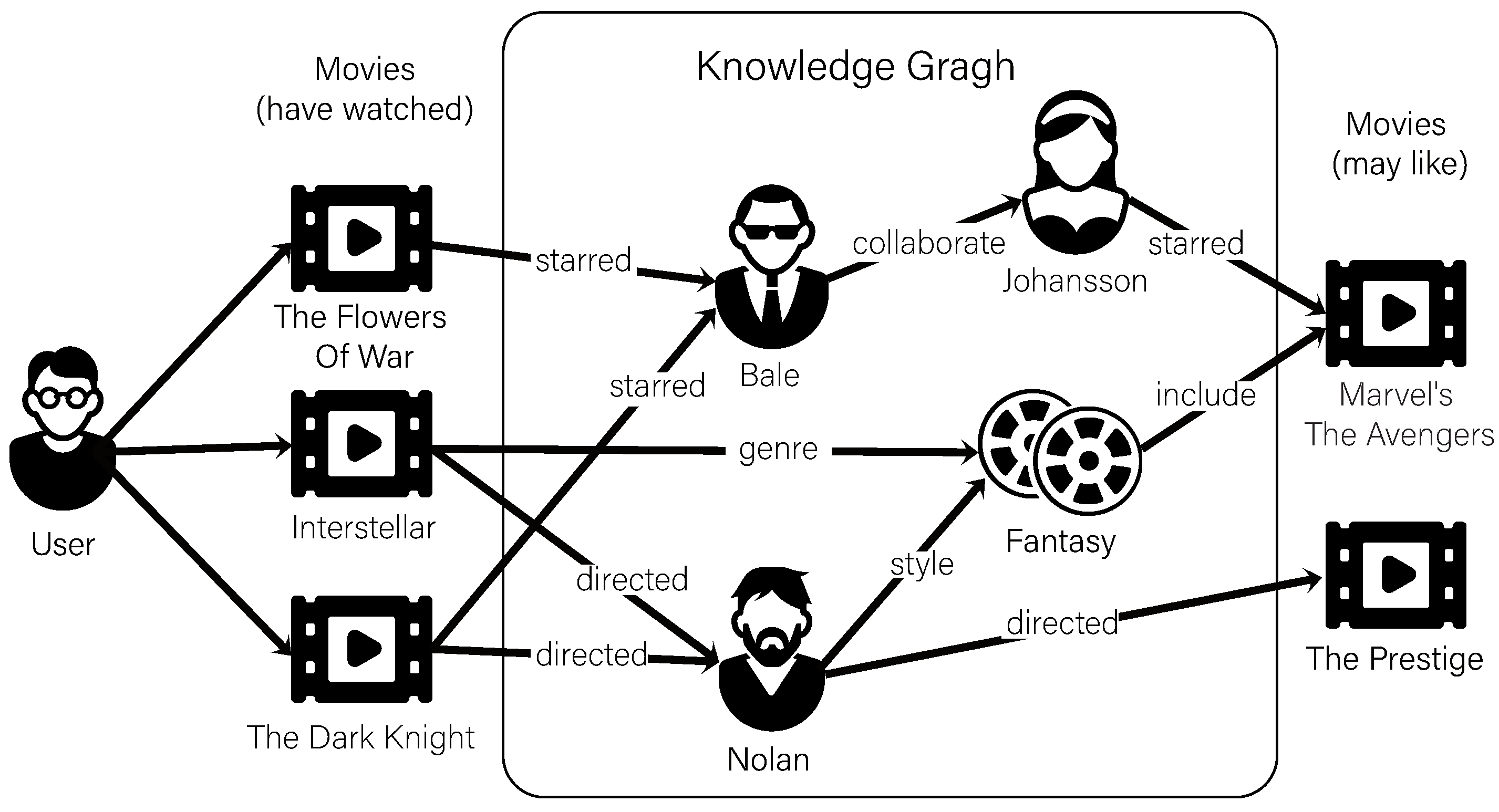
Our work is based on the knowledge graph for extraction of users’ interest and items’ recommendation. We define the KG for a particular recommendation scenario as G = (E,R) = (h<e>, r<r>, t<e>), where E and R are entities and relations in the knowledge graph respectively and h<e>, r<r> and t<e> represent the head, relation and tail of a knowledge triple. In the recommendation scenario, the KG consists of a set of items and their related entities (such as item’s attributes, external knowledge, etc.). For example, for the <<Titanic>> (Titanic, film.film), the KG has a knowledge triple (Titanic, film.film.star, Leonardo) indicating that Leonardo DiCaprio is the star of the <<Titanic>>.

It is worth mentioning that our model is based on user-centered extraction through the knowledge graph. But the original knowledge graph does not include the user’s entity. In this work, we embed the user as a new entity type into the knowledge graph and define a new relation type to connect the users to interacted item entity. For example, Mike has seen <<Dark Knight>>, so we added a new triple (Mike,film.film.watch, The Dark Knight) in the KG of movie. The following

Table 1. List of key symbols.

Symbol	Meaning
U={$u_1$,$u_2$...}	Set of users
I={$i_1$,$i_2$...}	Set of items
M	User-item interaction matrix
G={E,R}	Knowledge graph
E={$e_i$,$e_j$...}	Set of entities
R={$r_{(i,j)}$,$r_{(j,k)}$...}	Set of relations
$e_j^{\left[h\right]}$	Entity representation of $e_j$ after the h-th aggregation update
$N_{e_j}$	The direct neighbor set of $e_j$ in KG
$N_{e_j}^n$	the neighborhood of $e_j$ in n-hop
$W_k^{(u,i)}$	The aggregate weight of each neighbor entity $e_k$ under a given user-item pair

shows the key symbols and their meanings in this paper.

3.2. Model Framework Introduction

The NACF model has four parts of input: the user $u\in U$, the item $i\in I$, the user–item interaction matrix M and the corresponding knowledge graph G. Under the above conditions, NACF discovers the potential interest of users in KG and extracts hidden features between the various entities.

Specifically, given the user ID u, the item ID i and the neighbor set $N_e$ of each entity in the KG, NACF predicts whether u has potential interest in the i that u has not contacted. The user’s neighbors of KG is composed of item entities in user–item interaction record. The whole process is to learn the following prediction function:

$$y(u,i)=F(u,i|w,G_{<E,R>})$$

(1)

where $y(u,i)$ represents the probability that user u will participate in item i, F represents the recommendation function and w represents the trainable parameter of F.

For each particular user–item pair, the neighbor features of the user are iteratively aggregated onto the entity $e_u$. It includes three steps: neighborhood construction, neighborhood aggregation and prediction.

(1)

Neighborhood Construction

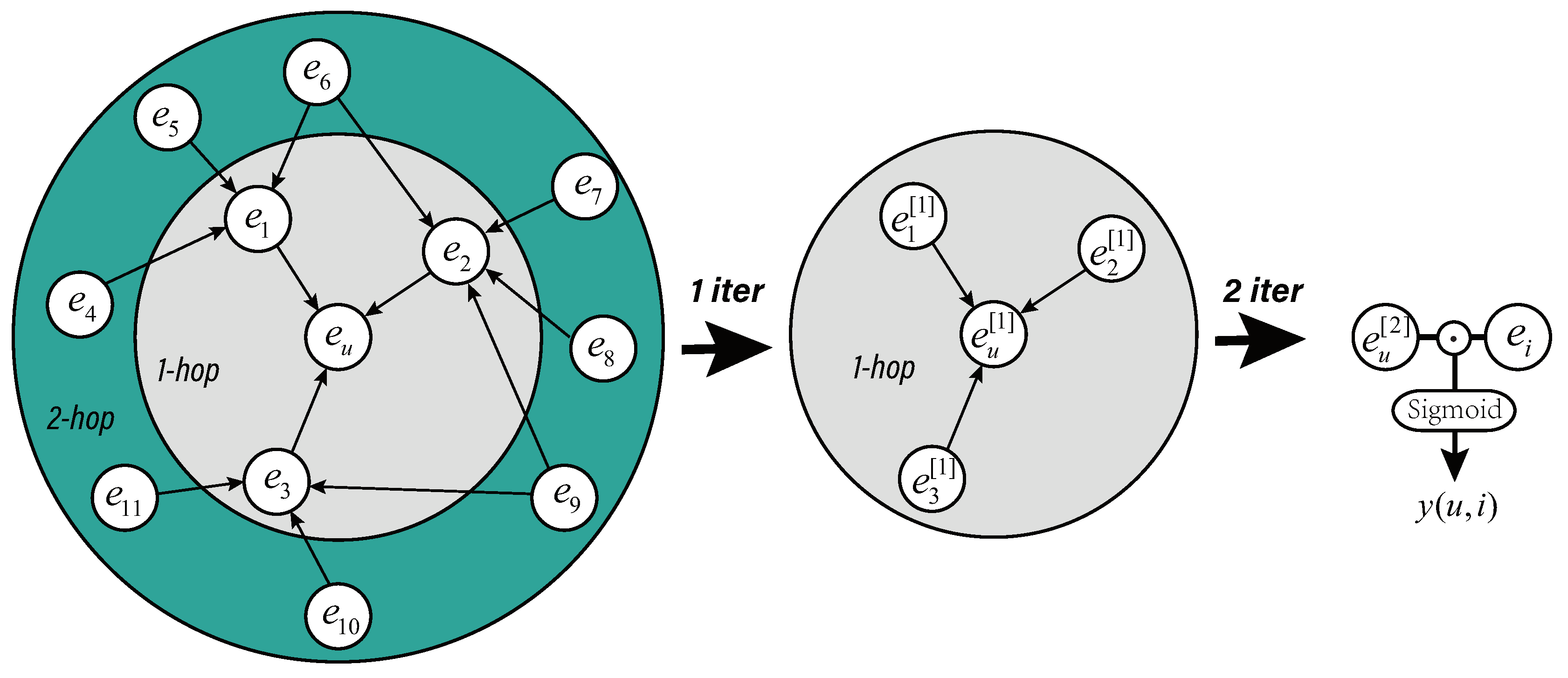
We take into account the entities in n-hop range of KG when extracting the users’ features. As shown in Figure 2 left sub-picture, the neighbors in the 1-hop range of $e_u$ ($N_{e_u}^1$) are composed of directly connected entities (items with interactive record), the neighbors in the 2-hop range ($N_{e_u}^2$) are composed of neighbors of directly connected entities in 1-hop and so on. Assuming the n-hop neighbor set of $e_u$ is $H_{e_u}^n$, neighborhood construction of $e_u$ is as follows:

$$N_{e_u}^n=\sum _{k=1}^n{H}_{e_u}^k$$

(2)

Such a construction method has the obvious advantage that the model expands the physical neighborhood through the KG and can explore the potential interests of the user more broadly and deeply. The range of neighborhood construction has a great impact on the final results of feature extraction. The goal of this step is to find the right range of neighborhood to fully exploit the potential knowledge without introducing too much noise.

(2)

Neighborhood Aggregation

Before neighborhood aggregation, NACF initializes all entities and relations as trainable and random vectors (d-dimensions). If the neighborhood of entity includes n-hop (n layers), the aggregation of the entity is iterated n times in total. In the h-th iteration, all entities in the n-h layer perform aggregation of neighboring information and update the embedding vector. After one aggregation operation is completed, the updated representation of entity comes from the fusion of itself and the neighboring entities. We call such an aggregation operation as sub-aggregation $Agg$. Until the model is iterated n times (the knowledge graph neighborhood converges to $e_u$), the neighborhood aggregation of user is complete.

In a n layer neighborhood, $e_u$ will update a total of n-1 times and the final representation of $e_u$ is $e_u^{\left[n\right]}$. For example, in a 2-hop aggregation scenario in Figure 2, the first iteration updates the $e_1$ to $e_1^{\left[1\right]}$, and the $e_u$ is updated to $e_u^{\left[1\right]}$, which we call the first-order representation of entity. In the second iteration, the $e_u^{\left[1\right]}$ is updated to $e_u^{\left[2\right]}$, which we call the second-order representation of entity. The specific sub-aggregation $Agg$ will be described in the Section 3.3.

(3)

Prediction

When the neighborhood aggregation of $e_u$ is completed, the user’s embedding entity $e_u^{\left[n\right]}$ and the item’s entity $e_i$ perform a point multiplication to generate a prediction score. Finally, this score will be normalized by the sigmoid function to the predicted click rate $y(u,i)$.

The NACF framework is shown in Algorithm 1:

Algorithm 1: NACF algorithm.

3.3. Aggregation Process

The aggregation of user-item pairs ($e_u$,$e_i$) includes the sub-aggregation of all entities in the current neighborhood $N_{e_u}^n$. Sub-aggregation is a single process of aggregating information from directly connected neighbors to entity. As shown in Algorithm 1, given user id u and item id i, we define the h-th sub-aggregation process Agg of $e_j$ as following:

$$e_j^{\left[h\right]}=Ag{g}_{(u,i)}\left(N_{e_j},e_j^{[h-1]}\right)$$

(3)

where $e_j\in N_{e_u}^{n-h}$ and $e_j^{\left[0\right]}$ is initial $e_j$.

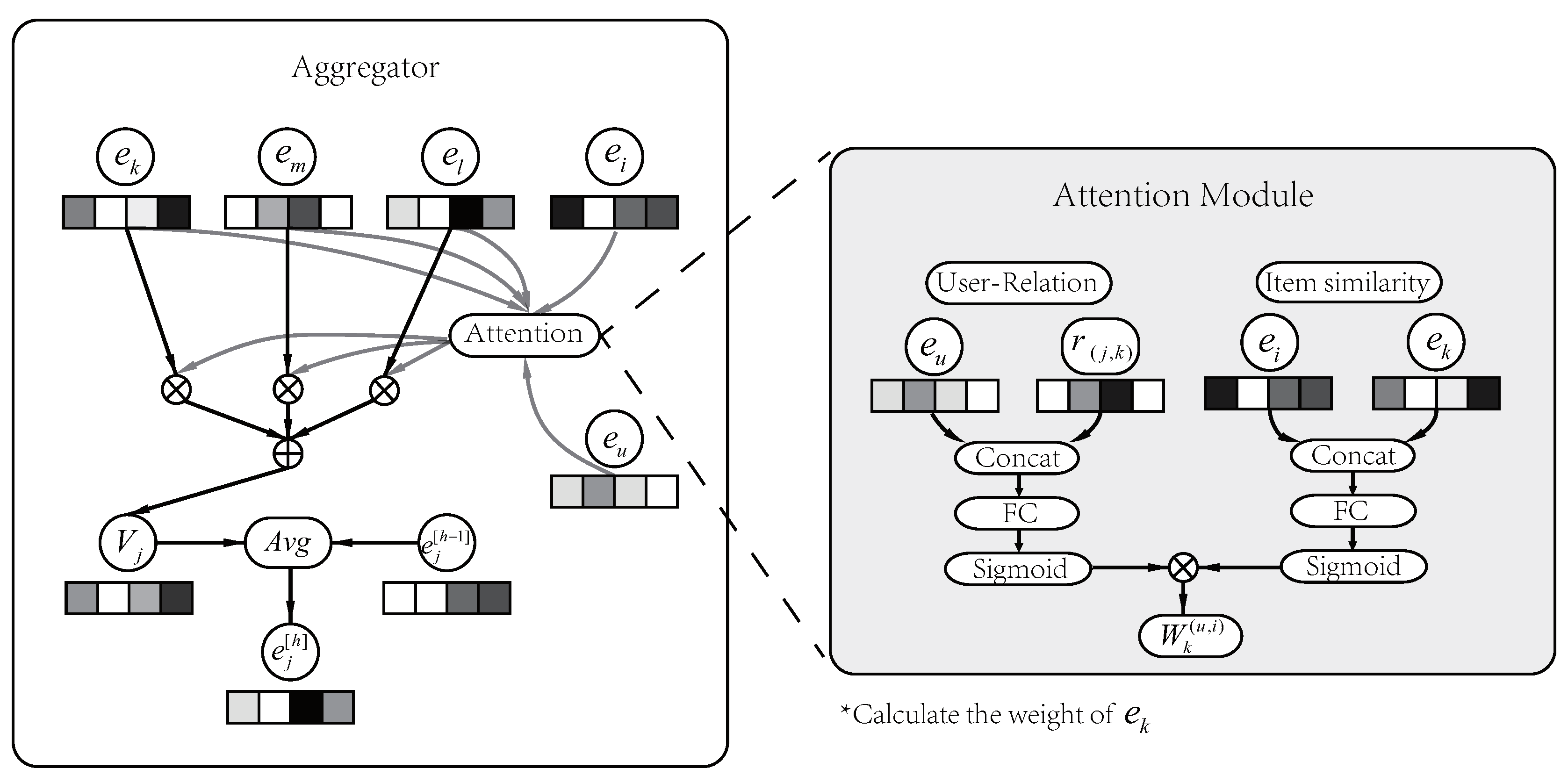
As shown in Figure 3, we use the neighboring sub-aggregation process of the $e_j$ as an example to illustrate the $Agg$ in NACF. We use $N_{e_j}$ to represent the collection of entities that are directly connected to $e_j$ and assume that $N_{e_j}=(e_k,e_m,e_l)$. $r_{(j,k)}$ represents the relation between $e_j$ and $e_k$. The corresponding link relations are $r_{(j,k)}$, $r_{(j,m)}$, $r_{(j,l)}$.

First we design a attention module to assign different weights to entities in the neighbor collection, since we believe that aggregation without distinction can introduce too much noise and is unreasonable. In NACF, we consider the degrees of users’ interest in different relations and the similarity between neighboring entities and recommended entity. In this way, the weights of different entities in the aggregation have been confirmed.

The attention module for calculating the weight is shown on the right sub-picture of Figure 3. For the weight calculation of the entity $e_k$, two parts of weight ($w_{(u,r)}$ and $w_{(e_i,e_k)}$) are calculated separately in the attention module. $w_{(u,r)}$ represents the user’s attention to $r_{(j,k)}$. For example, one user may be more inclined to choose a particular singer when listening to music; another may care more about the style of the music. $w_{(e_i,e_k)}$ is the similarity between the current neighbor $e_k$ and the recommended item $e_i$. We believe that entities with high similarity to recommended entity have a greater impact on user’s choice. Finally, the weight of neighboring entities $W_{e_k}^{(u,i)}$ is two-part ($w_{(u,r)}$ and $w_{(e_i,e_k)}$) multiplication result. The process is as follows:

$$w_{(u,r)}=Softmax\left(w_1·\left(concat\left(e_u,r_{(j,k)}\right)\right)+b_1\right)$$

(4)

$$w_{(e_i,e_k)}=Softmax\left(w_2·\left(concat\left(e_i,e_k\right)\right)+b_2\right)$$

(5)

$$W_k^{(u,i)}=w_{(u,r)}·w_{(e_i,e_k)}$$

(6)

where $w1$ and $w2$ are trainable vectors with $(2\times d)$-dimensions. $b_1$ and $b_2$ are one-dimensional trainable vectors.

In order to integrate the neighborhood information of $e_j$, we perform an cumulative operation on the weighted neighbors to generate an aggregated vector $V_j$. The final step of the sub-aggregation is to calculate the mean of the original entity representation $e_j^{[h-1]}$ and neighborhood representation $V_j$, and update the entity representation of $e_j$ to $e_j^{\left[h\right]}$. The update process of $e_j^{\left[h\right]}$ is as follows:

$$V_j=\sum _{e_k\in N_{e_j}}{W}_k^{(u,i)}·e_k$$

(7)

$$e_j^{\left[h\right]}=\left(V_j+e_j^{[h-1]}\right)/2$$

(8)

In the actual knowledge graph, there may be significant differences in the number of neighbors for each entity. To facilitate more efficient batch operation of the model, we extract a fixed-size neighbor set as a sample for each entity instead of its complete neighbor set. Specifically, the real neighborhood of the entity $e_j$ in the knowledge graph is $N\left(e_j\right)$. We set its calculation neighbor set to $S\left(e_j\right)$. $S\left(e_j\right)$ samples K neighbors from $N\left(e_j\right)$, and K is a hyper-parameter.

3.4. Complete Loss Function

In order to better learn the NACF parameters and knowledge graph embedding representation, we designed the following complete loss function:

$$Loss=\sum _{u,i}\phi \left(y(u,i),y{(u,i)}^{\prime }\right)+{\lambda }_1{\parallel w\parallel }_2^2+{\lambda }_2\left({\parallel E\parallel }_2^2+{\parallel R\parallel }_2^2\right)$$

(9)

The loss function is divided into three parts. The first part represents the model prediction loss, and $\phi$ is the cross entropy loss function. The second part is the $L2$ regularization of the trainable parameter w in the model. The third part is the $L2$ regularization of the knowledge graph embedding, where E and R are the embedding vectors of all entities and relations in KG respectively. ${\lambda }_1$ and ${\lambda }_2$ in $Loss$ are configurable hyper-parameters. Because the above optimization problem is complicated, we use Adam [29] to iteratively optimize the loss function. We will discuss the choice of hyper-parameters in the experimental section.

4. Experiments

4.1. Datasets Introduction

We used three datasets of movie (MovieLens-20M), music (Last.FM) and restaurant (Dianping-Food) in the experiment. The datasets is as follows:

• MovieLens-20M is a widely used dataset for movie recommendation and contains approximately 20 million clear ratings (from 1 to 5) on the MovieLens website. The corresponding KG contains 102,569 entities, 499,474 edges and 32 relation types.
• Last.FM contains listening records for 2000 users in the online music system. The corresponding KG contains 9366 entities, 15,518 edges and 60 relation types.
• Dianping-Food comes from Dianping.com, which contains more than 10 million user and restaurant interaction records (including clicks, purchases, etc.), with approximately 2 million users and 1362 restaurants participating. The corresponding KG contains 28,115 entities, 160,519 edges and seven relation types.

The knowledge graph corresponding to the datasets is derived from the pre-processing knowledge graph disclosed by KGCN [18] and KGNN-LS [30]. These works use Microsoft Satori to build KG for movie and music datasets. The knowledge graph of Dianping-Food comes from the brain of Meituan Brain which is the internal knowledge graph built by Meituan for dining and entertainment. In data preprocessing, we removed the items that are not in the knowledge graph. Before NACF starts training, we initialize all entities and relations as trainable and random vectors. They are constantly adjusted during training until convergence.

Since the MovieLens-20M and Last.FM are rating feedback, we convert them to click-through rate feedback. For movie, there are 6783276 records with 4–5 points and 6,718,346 records with 1–3 points. So we choose four as the click-through rate to achieve a better samples distribution. The ratings of the music are too sparse (from 1 to 352,698) to be used as a criterion for evaluating user interest. Thus, we set all the music that the user clicked as positive samples. To avoid a large gap between the number of positive and negative samples, we used negative sampling during training to randomly select negative samples from items that were not interacted by users in the datasets until the numbers of positive and negative samples were the same.

The statistics of these three data sets are shown in

Table 2. Statistics of the datasets.

	MovieLens-20M	Last.FM	Dianping-Food
#Users	138,159	1872	2,298,698
#Items	16,954	3846	1362
#Interaction	13,501,622	42,346	23,416,418
#Entities	102,569	9366	28,115
#Relations	32	60	7
#KG triples	499,474	15,518	160,519

.

4.2. Experimental Setup and Parameters

We selected two classical recommendation algorithms and three recommendation algorithms combined with KG as the baseline to compare the performance of NACF on the three datasets. The baselines are as follows:

• SVD [31] is a classic CF-based algorithm that uses inner product to model user-item interactions.
• LibFM [32] is a feature-based factorization model widely used for CTR prediction. In this experiment, TransR [33] was used to learn entity embedding for LibFM.
• CKE [7] combines collaborative filtering with knowledge embedding, text embedding, and item image embedding in a unified Bayesian framework. In this experiment, we represent each item only as an embedded vector learned by the TransR because the text descriptions and images in the datasets are not available.
• RippleNet [23] is a hybrid approach that uses KG information to assist recommendation, which spreads the user’s potential preferences on KG for CTR recommendations. In this work, we use the TransE algorithm [34] to learn entity embedding.
• KGCN [18] is a recommendation algorithm that uses GCN to convolve item features, which makes use of the knowledge graph to extract item potential associations.

The code of NACF is implemented under Python 3.7, tensorflow-gpu 1.12.0 and NumPy 1.15.4. Experimental hardware environment includes AMD R5 2600, GTX 1070 and 16G memory. We set the ratio of training, evaluation and testing sets to 6:2:2 and manually adjusted the hyper-parameters of the NACF according to area under curve (AUC). Both the ${\lambda }_1$ and ${\lambda }_2$ in the loss function were set to 0.001. The hyper-parameters of NACF are shown in

Table 3. Hyper-parameter settings.

	MovieLens-20M	Last.FM	Dianping-Food
#Neighbor	4	4	4
#Dimension	32	64	32
#hop	2	1	2
#Batch_size	1024	256	1024
#Epoch	10	10	10
#learning rate	$2\times {10}^{-2}$	$5\times {10}^{-4}$	$2\times {10}^{-2}$

.

4.3. Experimental Results

In order to verify the performance of NACF, we compared NACF with baselines in top-k recommendation and CTR prediction. In the top-k recommendation, the trained model selects K items with the highest click rate for each user of the testing set, and evaluates the selected items of the model with Recall@K Precision@K and NDCG@K (K∈ 1, 2, 5, 10, 50, 100). In CTR, we use area under curve (AUC), accuracy (ACC) and F1 score as metrics to evaluate the performances of all models. All experiments are conducted four times; the average values of the metrics are calculated.

The performances of all models in the top-k recommendation and CTR prediction are shown in Figure 4 and

Table 4. Performance in CTR.

	Movielens-20M			Last.FM			Dianping-Food
Method	AUC	ACC	F1	AUC	ACC	F1	AUC	ACC	F1
SVD	0.963	0.91	0.917	0.769	0.693	0.697	0.838	0.753	0.757
libFM	0.959	0.903	0.915	0.778	0.706	0.707	0.837	0.759	0.764
CKE	0.924	0.879	0.876	0.744	0.682	0.674	0.802	0.71	0.702
Ripple	0.968	0.921	0.914	0.78	0.702	0.709	0.833	0.751	0.758
KGCN	0.978	0.931	0.933	0.796	0.728	0.721	0.849	0.762	0.771
NACF	0.983	0.940	0.938	0.821	0.746	0.741	0.882	0.792	0.795
Improvement	0.51%	0.96%	0.53%	3.14%	2.47%	2.77%	3.87%	3.93%	3.11%

. We can observe:

(1)

As shown in Figure 4, NACF achieve optimal performance in the top-k recommendation of three datasets. Specifically, NACF outperforms the best of baselines by 16.48%, 10.62% and 24.88% in Recall@20 on the movie, music and restaurant sets, respectively. It also achieved 15.30%, 24.43% and 17.51% performance lead in Precision@10. In NDCG@10, NACF took the lead by 8.11%, 18.37% and 9.60% respectively. It shows that NACF can make good use of knowledge graph to assist recommendation in TOP-K scenarios.

(2)

In the CTR prediction, Table 4 shows that NACF achieved leading performance in AUC, ACC and F1. But the improvement is not very great, especially in movie. For music, the improvement of metrics is better than for movie. It shows that NACF can solve the sparsity problem to a certain extent, since Last.FM is much sparser than Movielens-20M and Dianping-Food.

(3)

The performances of NACF, KGCN and RippleNet are basically ahead of CKE, SVD and libFM. It is worth mentioning that KGCN and Ripple also use the multi-hop neighborhood of KG, which illustrates that extracting multi-hop information in KG is necessary for recommendation. The CKE model performed very poorly in our experiments. It proves that CKE cannot make full use of KG with KGE algorithm like transR.

4.4. Performance Analysis

(1)

Cold Start Problem

In this subsection, we verify that introducing KG into the recommendation can effectively alleviate the cold start problem. We gradually reduced the size of the MovieLens-20M training set from r = 100% to r = 20% (evaluation set and test set unchanged) to study the performances of models in cold start scenario. The results of AUC are shown in Figure 5. When r = 20%, the AUCs of the five baselines decreased by 7.5%, 5.9%, 2.8%, 4.8% and 1.9% respectively. The performance of NACF decreased by only 1.6%. This shows that NACF can achieve better result than baselines in a cold start scenario.

At the same time, we observe that the recommendation models based on KG performed better on the cold start problem than the classic models. This phenomenon verifies the effectiveness of KG information to alleviate the cold start problem.

(2)

Effect of attention mechanism

Next, we study the effectiveness of the proposed attention module. We have mentioned that the attention module calculates the weights of the two parts weights $w_{(u,r)}$ and $w_{(e_i,e_k)}$ respectively in Section 3. $w_{(u,r)}$ represents the user’s interest in the entities’ current relation. $w_{(e_i,e_k)}$ is the similarity between the current neighbor $e_k$ and the recommended item $e_i$. As shown in Figure 6, we observed the impact of different attention mechanisms on the Recall@20 in three datasets.

NACF-Mean means the NACF without attention module. In the sub-aggregation process, the calculation of $V_j$ is to average the representation vector of neighbors. NACF-Rel and NACF-Item only use $w_{(u,r)}$ or $w_{(e_i,e_k)}$ respectively. NACF-Att represents the model that uses the full attention module. We observed that all models using attention mechanisms performed better than NACF-Mean. Moreover, the Recall@20 performance of NACF-Item and NACF-Rel is lower than when them combined. We specifically observe the performance of the model in the MovieLens-20M. Compared with NACF-Mean, NACF-Item and NACF-Rel increased by 7.47% and 4.95% respectively, and NACF-Att had a performance improvement of 10.35%. These results validate the effectiveness of the proposed attention module. In neighborhood information aggregation of KG, it is helpful that consider the user’s interest in different relations and the similarity between entities.

(3)

Impacts of different embedded dimensions

We analyzed the effects of different embedding dimensions of entity on NACF performance. The performances in the three datasets are shown in

Table 5. Effects of different embedded dimensions on AUC.

Dim	8	16	32	64	128
Movielens-20M	0.98	0.981	0.983	0.981	0.978
Last.FM	0.818	0.821	0..827	0.829	0.825
Dianping-Food	0.878	0.88	0.882	0.879	0.876

. When other parameters unchanged, the AUC of NACF will gradually rise with the increasing of the dimension d and achieve the optimal performance in 32-dimension or 64-dimension. But as the dimension gets larger, the performance gradually declines. That indicates that too large an embedding dimension may lead to over-fitting of NACF.

(4)

Impact of Different Neighbor Samples

We study the performance of NACF in different neighbor size by changing the number of neighboring samples K. As shown in the following

Table 6. Impact of different neighbor samples on AUC.

Neighbors	2	4	8	16	32
Movielens-20M	0.98	0.983	0.982	0.981	0.978
Last.FM	0.825	0.829	0.827	0.823	0.819
Dianping-Food	0.878	0.882	0.88	0.879	0.876

, NACF gets the best performance in all three datasets when sampling four neighbors. It shows that too small a neighboring size K will make the model unable to extract enough knowledge information, while too large a K will introduce too much noise and cause a slight decline in performance.

(5)

Impact of different neighborhood layers

We also analyze the effects of different sampling layers on the performance of the model. According to the NACF framework, more neighborhood layers will result in a geometric increase in the number of entities participating in calculation. The run time of NACF will also increase significantly. But the performance of the model does not increase gradually. As shown in

Table 7. Effect of different sampling layers on AUC.

Layers	1	2	3	4
Movielens-20M	0.979	0.983	0.974	0.963
Last.FM	0.829	0.821	0.807	0.794
Dianping-Food	0.874	0.882	0.869	0.853

, both the movie and restaurant achieve optimal performance when sampling layers is 2, and the Last.FM performs best when sampling layers is 1. Thus, the NACF needs a certain neighborhood to aggregate information. However, the larger sampling layers will introduce too many weakly related entities to participate in the aggregation and reduce the performance of the model.

5. Conclusions

In this paper, we use neighborhood information of knowledge graph to aid the recommendation. We design a new recommendation framework NACF to incorporate the user’s neighborhood information into collaborative filtering. The innovation of NACF is biased aggregation of neighborhood. It makes full use of structure of knowledge graph to extract features of user’s interest, and introduces an attention mechanism to assign weights to different aggregate information. We conducted a large number of experiments on three public datasets and analyzed the rationality and effectiveness of using KG to assist the recommendation. It is verified that NACF has a performance level ahead of existing algorithms.

In future research, we will improve NACF and try to introduce other assistant information to understand users’ behavior. For instance, semantic analysis combined with user comments, social networks, etc. We need try more ways of learning in feature mapping based on the knowledge graph, such as spectral GCN, graph attention network, more subtle attention mechanisms, etc. We will also focus on user online behavior analysis to achieve more effective and interpretable recommendations.