A Hybrid Model to Simulate Test Cases of Electrical Power Systems

Abstract

The development of solution algorithms for power system problems is based on hypothetical test systems and test cases. These systems are very scarce, and the degree of variability is relatively low. The constant development of the economic analysis in electrical power systems denotes the need to obtain standardized systems and cases. In this study, the creation of standardized test cases based on a hybrid model using Lévy alpha stable distributions and generalized additive models is proposed. The objective of the work is to present a methodological proposal for the creation of test environments for optimization models based on general information about the operation of particular power systems. The simulation of random values based on Lévy alpha stable distributions lets capturing the series impulsivity and demand peaks, and the use of generalized additive models permits capturing non-linearity in the behavior of the demand for electrical energy. The hybrid model will tolerate simulating as many instances as necessary, with a coherent behavior attached to the reality of the operation of the analyzed electrical systems.

1. Introduction

The problem of economic dispatch has generated a wide development in the optimization algorithms for its solution as well as the adequate planning of the generation and expansion of the electrical networks. Its importance is such that in the literature, multiple approaches have been developed in this regard. However, there is a need to have available information from test systems for such algorithms; in most cases, the information available from real electrical networks is not public, so being able to have a robust method for generating test data efficiently represents a relevant contribution. This paper proposes a conceptual framework based on a hybrid model using Lévy alpha stable distributions and generalized additive models for the generation of test cases.

One of the essential inputs to test the optimization algorithms are the test cases for the behavior of the demand; without such input, it is impossible to test the efficiency of the implemented algorithms. This work contributes to having standardized test cases that can be used to benchmark the performance of many proposed optimization techniques. One of the main advantages of the proposed method to generate test instances is, once obtained, the model parameters can create as many instances as needed without losing robustness in the estimates. This would be equivalent to evaluating the optimization model in a variety of electrical systems. This represents a great advantage over other techniques. Being able to have unlimited test instances will let to analyze in greater detail the robustness of the optimization algorithms used as well as their stability in obtaining feasible solutions.

The study of the problem of economic dispatch has been an area in continuous development, integrating aspects such as renewable energy, distributed generation, and smart grids into the electricity grid. However, there has not been much attention in the generation of test systems for the evaluation of optimization algorithms. They are generally considered historical data, or random instances are generated assuming a Normal probability distribution. Both proposals have some disadvantages, the use of historical data limits the availability of information, especially in recently created systems or with innovative elements, as well as limiting the number of available instances. In the case of the generation of random instances through normal distribution, it implies some limitations, such as the presence of heavy tails in historical data. Additionally, when generating random numbers through the normal distribution, the seasonal behavior of the characteristic demand of electrical systems is lost. Therefore, it is difficult to replicate medium and long-term power generation planning periods. This avoids reflecting the response of the economic dispatch models to extreme values and seasonality, thus limiting the conclusions on the solutions found.

The proposed hybrid model of this work seeks to overcome these limitations in test cases by using the alpha stable distribution and using generalized additive models. The proposal is integrated in the following way, fitting of historical data to the stable alpha distribution seeks to identify the presence of impulsivity in the data series. With this, it is possible to simulate random instances that follow the alpha stable distribution. For the integration of the non-linear component, the simulated alpha stable data is integrated into a generalized additive model, which consents to segment the data into additive modules, each fitted to a particular non-linear function (such as the spline or kernel functions). Thus, the generated instances considering extreme scenarios as well as replicating the non-linear seasonal behavior of the electrical system analyzed.

The structure of the work is as follows: Section 2 presents a literature review of different aspects in the solution of the problem of economic dispatch as well as state of the art on the generation of test cases. Section 3 explains the proposed methodology that integrates a brief generic description of the economic dispatch problem, the definition of the alpha stable distribution, and the simulation of alpha stable random numbers. Further to addressing the theoretical foundations of generalized additive models. Section 4 describes the application of the model in three generic electrical systems for the simulation of test cases in an operational year of 52 weeks. Finally, Section 5 presents the conclusions.

2. Literature Review

The optimization problems for electrical power systems have been studied for more than five decades. A definition of economic dispatch is the operation of generation facilities to produce energy at the lowest cost to reliably serve consumers, recognizing any operational limits of generation and transmission facilities. In the typical unit commitment [1], the problem consists as determining the mix of generators and their estimated output level to meet the expected demand of electricity over a given time horizon (a day or a week) while satisfying the load demand, spinning reserve requirement and transmission network constraints. An electric network consists of many generation nodes with various generating capacities and cost functions, lines of transmission, and nodes of power demand [2].

The application of optimization models for electrical power systems is marked by constant development for new algorithms like exact methods, metaheuristics, and hybrid strategies [3]. Authors such as Montoya O. [4] show applications of a non-linear economic dispatch problem and its implementation in commercial software for operational and regulatory analyses in Colombia. Other works, such as Perez-Lechuca et al. [5], show the application of an optimization model for hydrothermal coordination and the emission of polluting particles. Recent research integrates various sources of fuel, such as natural gas, in the determination of the optimal generation at the lowest cost, considering wind generation, in addition to considering the model as a bi-level model [6]. Jin X. et al. [7] shows a dynamic version of the problem of economic dispatch, considering a hybrid energy micro-grid, and adding to the problem a virtual energy storage system.

The problem has approached from the perspective of the integration of renewable energies. As well as different methods of solving the optimization problem, such as the case of Qu B.Y. et al. [8], where the application of multi-objective evolutionary algorithms models is shown for the solution of an environmental-economic dispatch problem. In the same way, different versions of the problem of economic dispatch have been explored through the temporality of the solution. Depending on the demand period that is desired to be planned, in Jiang Y. et al. [9], a stochastic version of the problem of economic dispatch is shown, considering wind energy and demand response for scheduling of home energy management. Other authors include in the problem constraints related to the emission of pollutants as well as risk measures in the electrical system. Perez-Lechuga et al. [5] propose a multi-objective model of economic dispatch with restrictions on risks arising from the integration of wind energy into the system. Similarly, economic dispatch models with multiple energy carriers have proposed, in this case, works such as Derafshi-Beigvand S. et al. [10], which address the treatment of energy hubs in the operation of integrated systems using a particle-swarm optimization algorithm.

The approach to the problem of economic dispatch has multiple aspects, among which the solution method and the characteristics of the analyzed electrical system can highlight. Recent research shows the integration of clean energy as well as energy storage and multiple energy carriers. The problem of economic dispatch is and will continue to be a priority problem in the academic and industrial fields because electrical systems evolve under the availability of energy in the world and with technological development.

Along with the development of novel algorithms for solving the problem of economic dispatch in its multiple variants, it is necessary to have test systems to evaluate solution algorithms. The electricity network, as well as the characteristics of the operation of an electrical system, are reserved information. Generally, there are test versions of electrical systems as well as characteristics of the network’s demand behavior. To benchmark the performance and solution quality for any solution technique, it is necessary to have a variety of electrical test systems [11]. Nowadays, we still lack the existence of standardized test systems that can be used to benchmark the performance and solution quality of proposed techniques. Many papers consider different test systems, which make it very difficult to perform a proper comparison between methods that have proposed [12]. Zhang X.P. et al. [13] have referred that the existing IEEE test systems developed are used for reliability, power flows, and stability analyses but not for economic analysis. Recently, some panels focusing on the development of standard test systems of transmission and distribution systems for economic analysis have emerged. In 2007, the IEEE Working Group (WG) on Test Systems for Economic Analysis was created, sponsored by the IEEE System Economics subcommittee. As a result of this initiative, Peña I. et al. [14] proposed a version of the IEEE 18-bus test system, a database of an electrical network, with a reconfiguration of three regions of the US Western Interconnection, including renewable energies. A test system includes transmission, generation, load, wind, and solar data. Barrows C. et al. [15] proposed an update of the IEEE reliability test system, which includes the production of electricity, transmission, and consumption needs, but the last update of this test system was carried out in 1996. The modifications include the inclusion of geographic information of Southwestern United States to include temporal space information wind, solar, and load data with forecasts. Mahdavi M. et al. [16] presented a proposal for a test system based on real data, which has planning information for network expansion, operation, and reliability. This work integrates information on the expansion of the generation by providing detailed information on the architecture of the electricity grid. The presented load modeling includes hourly, daily, weekly, monthly, and seasonal patterns.

The existing test systems consider the architecture of an electrical system, in addition to the recent updates to have renewable energies, as well as information on generation and consumption planning. There are few cases where demand information is included; these systems are input for testing the different economic dispatch models to implement. A fundamental characteristic to test the different algorithms for solving the problem of economic dispatch lies in the treatment of the demand that determines the optimal allocation at the lowest cost. Several authors have documented the seasonal nature of the demand for electrical energy, as well as the availability of fuels and renewable energy in the planning of expansion [17,18,19,20,21]. For the forecast of the demand for electric energy, there are multiple methodologies. These methodologies are based generally on time series models, machine learning, wavelets theory, multi-agent, or hybrid models [22,23,24,25,26,27,28]. The objective of these models is to forecast as accurately as possible the demand for electric power for a period forward based on the available historical information. The drawback of using this forecasted data to test algorithms for solving the economic dispatch problem is that it is a particular data that considers a specific time horizon and is according to the available information. Therefore, the use of a demand simulation method based on the use of alpha stable distributions and generalized additive models is another option for testing and validating algorithms in a development phase.

It has been identified that electrical demand presents a greater degree of impulsivity due to the presence of peaks in the series during the hours of the day and seasons of high-energy demand in the year [24,25,26,27,28]. For this, we use the Chambers–Mallows–Stuck algorithm for simulating alpha stable random variables characterizing demand peaks and generalized additive models (GAMs) to model the non-linear behavior of real electrical systems. This proposal allows us to model the real behavior of the electrical demand and build possible extreme scenarios. Each scenario corresponds to a price-elastic demand curve. The simulations are based on real observations of demand for different reliability test systems. Electrical network data are taken from P.M. Subcommittee [29] and 118 bus IEEE test systems from Christie R. et al. [30], and a portion of the electric energy system of mainland Spain from Alguacil N. and Conejo J.A. [31].

According to the literature review, there are areas of opportunity for the generation of test cases, especially for the academic field, due to the scarcity of public information available on the architecture of electrical networks, as well as their operation. Therefore, having a method to simulate instances is of potential utility for the development of research in power systems. Most of the existing methods focus on forecasting electricity demand, but it is necessary to take into account the structure of the electrical system in the generation of test cases. That is the reason why the proposed hybrid model could provide additional information to the current state of the art.

3. Materials and Methods

This section briefly describes the different methodologies used to build the hybrid model by describing the problem of economic dispatch, simulation methodology with alpha stable distribution, and generalized additive models for the fitting of non-linear behaviors in the data series.

3.1. Short Version of Economic Dispatch Problem

The problem of economic dispatch of power plants is a classic problem in power systems. We have a network of electric power generators that are located in different nodes of an electric network. The objective of the problem is to determine, for a given period, the power that each generator has to produce to meet the required demand at the minimum cost, complying with a set of technical restrictions of the network and the generators. Each line in the network transmits power from the supply node to the receiving node. The power sent is proportional to the difference in the angles of these nodes (susceptance). The power transmitted from node $i$ to node $j$ through line $(i-j)$ is represented by Equation (1) [32]:

$$B_{ij}({\delta }_i-{\delta }_j)$$

(1)

where $B_{ij}$ is the susceptance of the line $(i-j)$, ${\delta }_i$ and ${\delta }_j$ are the angles of the nodes. The amount of power transmitted through a network line is limited by thermal or stability conditions. This is represented in Equation (2).

$$-P_{ij}^{max}\le B_{ij}({\delta }_i-{\delta }_j)\le P_{ij}^{max}$$

(2)

The power produced by a generator is a magnitude limited lower and higher. The lower level is due to stability conditions and the upper level to thermal conditions. Equation (3) shows this constraint

$$P_i^{min}\le P_i\le P_i^{max}$$

(3)

where $p_i$ is the power produced by generator $i$ and, $P_i^{min}$ and $P_i^{max}$ are the maximum and minimum power output that can be administered to generator $i$. In each node, the power must match the power that comes out of it according to the law of conservation of energy. This is represented in Equation (4).

$${\displaystyle \sum }_{j\in {\mathsf{\Omega }}_i}{B}_{ij}({\delta }_j-{\delta }_i)+p_i=D_i, \forall i$$

(4)

where ${\mathsf{\Omega }}_i$ is the set of nodes connected through the lines to node $i$ and $D_i$ the demand in node $i$, the transmitted power is bounded. Equation (5) show this constraint.

$$-P_{ij}^{max}\le B_{ij}({\delta }_i-{\delta }_j)\le P_{ij}^{max},\forall \mathrm{j}\in {\mathsf{\Omega }}_i,\forall i$$

(5)

Therefore, a generic version of the problem of economic dispatch can be formulated as follows. Equation (6) shows the objective function of the economic dispatch problem [32].

$$MinZ={\displaystyle \sum }_{i=1}^n{C}_i{p}_i$$

(6)

where $C_i$ is the production price of generator $i$ and $n$ number of generators. Subject to generic constraints represented by Equations (7)–(10)

$${\displaystyle \sum }_{j\in {\mathsf{\Omega }}_i}{B}_{ij}({\delta }_j-{\delta }_i)+p_i=D_i;i=1,2,\dots ,n$$

(7)

$$-P_{ij}^{max}\le B_{ij}({\delta }_i-{\delta }_j)\le P_{ij}^{max};\forall \mathrm{j}\in {\mathsf{\Omega }}_i,i=1,2,\dots ,n$$

(8)

$$P_i^{min}\le P_i\le P_i^{max};i=1,2,\dots ,n$$

(9)

$${\delta }_k=0;where k is an arbitrary node$$

(10)

where

$n:$ the number of generators

$P_i^{min}:$ the minimum power of generator $i$

$P_i^{max}:$ the maximum power of generator $i$

$B_{ij}:$ the susceptance of line $i-j$

$P_{ij}^{max}:$ the maximum transport capacity of line $i-j$

$C_i:$ the cost of producing power from generator $i$

${\mathsf{\Omega }}_i:$ the set of nodes connected to node $i$

$D_i:$ the demand at node $i$

$p_i:$ the power to be produced by generator $i$

${\delta }_i:$ the angle of node

As documented in the first section, the problem of economic dispatch has multiple aspects according to the elements that are to be integrated into the power grid to be modeled. The demand of each node in the network is a fundamental element for this optimization problem; this variable is generally determined based on historical data observed. However, when proposing new methods of solving the problem and assessing its efficiency and stability, it is necessary to have a large number of test cases that replicate in the best way the real behavior of the electrical network.

3.2. Stable Distributions

There are multiple applications of this family of distributions in many sectors. Lévy P. [33] was the first to develop a stable distribution theory. Later, Mandelbrot B. [34] proposed a theory based on this distribution to solve the problem of price fluctuations. There are some issues in operating these distributions as they lack an analytical form. A random variable $W$ has stable distribution $X~S(\alpha , \beta , \gamma , \delta ;1)$ with the characteristic function represented by Equation (11) [35].

$$\mathrm{E}\exp (itW)=\left\{\begin{array}{c}\exp \left\{-{\gamma }^{\alpha }{\left|t\right|}^{\alpha }\left[1-i(sgn(t))\beta (tan\frac{\pi \alpha }{2})\right]+i\delta t\right\},(\alpha \ne 1)\\ \exp \left\{-\gamma \left|t\right|\left[1+i(sgn(t))\beta \frac{2}{\pi }\ln (\left|t\right|)\right]+i\delta t\right\},(\alpha =1)\end{array}\right\}$$

(11)

where $sgn(x)=\left\{\begin{array}{c}1 if x>0\\ 0 if x=0\\ -1 if x<0\end{array}\right\}$ and $\alpha ϵ(0,2]$ represents the impulsiveness of the random variable. The parameter $\beta \in \left[-1,1\right]$ is the symmetry of the distribution. $\gamma >0$ is a scale parameter, and $\delta \in R$ is the position parameter. Alpha-stable distribution with different parameters defines known distribution functions, Gaussian distribution in Equation (12), Cauchy distribution in Equation (13), and Lévy distribution in Equation (14).

$f_{2,0}(.|\gamma ,\mu )$ is a Gaussian distribution with mean $\delta$ and variance $2{\gamma }^2$,

$$N(x,\mu 2{\gamma }^2)=\frac{1}{2\gamma \sqrt{\pi }}\exp \left\{\frac{{(x-\mu )}^2}{4{\gamma }^2}\right\}$$

(12)

$f_{1,0}(.|\gamma ,\mu )$ is a Cauchy distribution with density,

$$pCauchy(x|\mu ,\gamma )=p\frac{\gamma }{\pi ({(x-\mu )}^2+{\gamma }^2)}$$

(13)

$f_{1/2,1}(.|\gamma ,\mu )$ is a Lévy distribution with density,

$$pLévy(x|\mu ,\gamma )={(\frac{\gamma }{2\pi })}^{\frac{1}{2}}\frac{1}{{(x-\mu )}^{\frac{3}{2}}}exp\left\{-\frac{\gamma }{2(x-\mu )}\right\}$$

(14)

In this research, we use Nolan’s algorithm to estimate the alpha-stable distribution parameters. Nolan’s algorithm [36] is based on Zotolarev’s representation of the characteristic function [37]. The algorithm performs the numerical integration of a set of splits of the random variable domain. These splits are based on the sign change of the trigonometric functions (sine and cosine) that result from the transformation of Zoratev V.’s [37] representation into the complex plane. There are other methodologies for estimating the parameters of the stable distribution, like those presented by Belov I. [38], proposing a combination of Gaussian and Laguerre’s quadrature; or Mittnik S. et al. [39] presenting an algorithm that applies the fast Fourier transform. Finally, DuMouchel W.H. [40] used a Bergström series expansion on Zotolarev’s characteristic function representation for approximating a stable cumulative distribution. Nevertheless, Nolan’s algorithm [35,41] has proven to be an easy method to implement, with good performance with high-frequency data, as is the case with the demand for electrical energy.

3.3. Stable Random Variable Simulation

The Chambers–Mallows–Stuck method [42] generates a random variable $X$ with distribution $f_{\alpha ,\beta }(X|1,0)$ from a non-linear transformation of two random variables independently, one uniform $(V)$ and another exponential $(W),$ using the following theorem. Let (V) be a uniform random variable in the interval $(\frac{-\pi }{2}, \frac{\pi }{2}),$ and $(W),$ an exponential random variable with mean equal one, if $V$ and $W$ are independent. Equation (15) displays a random variable that follows an alpha stable distribution.

$$\mathrm{X}=S_{\alpha ,\beta }\frac{\sin (\alpha (V+B_{\alpha ,\beta }))}{{(cosV)}^{\frac{1}{\alpha }}}{(\frac{cos((1-\alpha )V+B_{\alpha ,\beta }\alpha }{W})}^{\frac{(1-\alpha )}{\alpha }},$$

(15)

follows a stable distribution with $f_{\alpha , \beta }(X|1,0)$, where $B_{\alpha ,\beta }$ and $S_{\alpha ,\beta }$ are defined by Equations (16)–(17).

$$B_{\alpha ,\beta }=\frac{\arctan (\beta \tan (\frac{\pi \alpha }{2}))}{\alpha }$$

(16)

$$S_{\alpha ,\beta }={(1+{\beta }^{2}ta{n}^2\frac{\pi \alpha }{2})}^{\frac{1}{2\alpha }}$$

(17)

Once the variable $(X)$, is estimated, a variable that follows stable distribution for any set of values of the parameters $S(\alpha ,\beta ,\gamma ,\delta and\mu )$ is generated by Equations (18)–(19).

$$f_{\alpha ,\beta }(\gamma ,\mu )~\gamma X+\mu si\alpha \ne 1,\mathrm{and}$$

(18)

$$f_{\alpha ,\beta }(\gamma ,\mu )~\gamma X+\frac{2}{\pi }\beta \gamma ln\gamma +\mu , if \alpha =1$$

(19)

Some examples of the application of Chambers–Mallows–Stuck are presented in [41,43,44], among other works.

3.4. Generalized Additive Models (GAMs)

The different methodologies for making predictions or forecasts using linear models have limitations when working with data that presents non-linear behavior. Recently the generalized additive models (GAMs) approach has been developed. These models are an extension of the regression models, with non-linear functions for the variables and maintaining the additivity of the model. GAMS models work with quantitative and qualitative response variables [45].

For the avobe, the regression model can be extended to capture non-linear relationships between independent variables and the dependent variable. For this, it is necessary to replace each linear component $({\beta }_j{x}_{ij})$ with a non-linear (smoothed) function $f_j(x_{ij})$. The model specification is presented by the Equations (20)–(21) [45].

$$y_i={\beta }_0+{\displaystyle \sum }_{j=1}^p{f}_j(x_{ij})+{\epsilon }_i$$

(20)

$$y_i={\beta }_0+f_1(x_{i1})+f_2(x_{i2})+\dots +f_p(x_{ip})+{\epsilon }_i.$$

(21)

where $f_j$ are smooth non-linear functions.

The type of functions that can be used includes natural splines, step functions, polynomial, smoothing splines, and basis functions. The use of different functions for non-linear treatment is so that each explanatory variable improves the efficiency of the estimates. Given the additive nature, it is feasible to analyze the effect of each independent variable separately, keeping the rest of the variables constants. This property is the one that will fit in a better measure of the seasonal behavior of the demand for electrical energy. The methods for estimating the parameters of the additive model are based on iterative algorithms, such as the back-fitting algorithm [45].

3.5. Proposed Hybrid Model

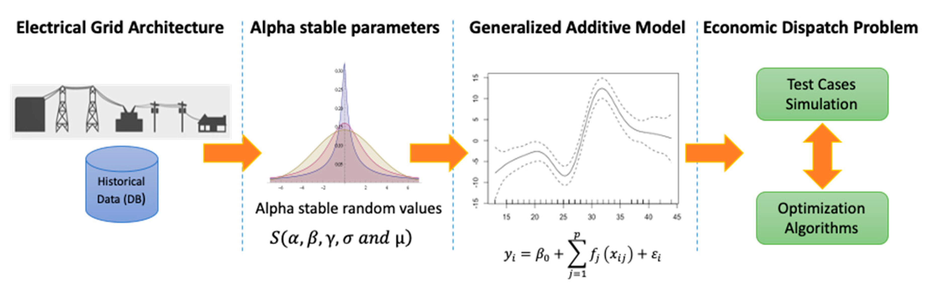
The proposed model considers the structure of a power grid, as well as historical demand data. Based on this information, the parameters of the alpha stable distribution are estimated. Subsequently, using the Chambers–Mallows–Stuck method [42], stable random values simulate as much data as necessary. Using the simulated information as a training base, a GAM model is fitted to estimate the demand for electricity in the desired time horizon. The conceptual proposal is presented in Figure 1.

The structure of the proposed model is based on the sequential estimation of a set of parameters for simulating the power system test cases. The first step is to fit the historical data from the reference power system to the stable alpha distribution using the regression method.

Let $(X_t)$ be a random variable that represents the demand for electrical energy for a period of time $(t)$. With these historical data, the parameters of the stable alpha distribution are estimated by the regression method using the following equations [35,36,46,47].

Estimation of parameters $\alpha and \gamma$, is presented in Equation (22).

$$y_k=m+{\alpha }_k+{\epsilon }_k, k=1, 2,\dots , K$$

(22)

where, $y_k=\log (-\log {(\phi (t_k))}^2$, $m=\log (2{\gamma }^{\alpha })$, $w_k=\log (t_k)$, ${\epsilon }_k$ is the random error, and $K$ of the historical data seats $t_k=\frac{\pi k}{25}$ $(k=1, 2, \dots , K)$. Whit estimations of $\alpha and \gamma$ is a possible estimate of the symmetric parameter $(\beta )$ and location parameter based on Equation (23).

$$Z_l={\mu }_{\mu l}-\beta {\gamma }^{\alpha }\tan (\frac{\pi \alpha }{2})sgn({\mu }_l){\left|{\mu }_l\right|}^{\alpha }+{\eta }_l, l=1, 2, \dots , L$$

(23)

where, $Z_l=g_n({\mu }_l)+\pi k_n({\mu }_l)$, $g_n(\mu )=\arctan \frac{(Im(\phi (\mu ))}{Re(\phi (\mu ))}$, ${\eta }_k$ is the random error, and $L$ of the real data sets ${\mu }_l=\frac{\pi l}{50}$ $(l=1, 2, \dots , L)$. The results of this stage are the parameters of the stable alpha distribution for the historical data series $X_t~S(\widehat{\alpha }, \widehat{\beta }, \widehat{\gamma }, \widehat{\delta })$. Using Equations (18) and (19) and the estimated stable alpha distribution parameters, stable alpha random numbers can be generated ${\widehat{X}}_n~S(\widehat{\alpha }, \widehat{\beta }, \widehat{\gamma }, \widehat{\delta })$. In order to estimate the GAM model, information on the operation of the power system is considered as the price of energy and the price of fuels for the time horizon to be modeled. In this case, fuel prices and the local marginal price will be used so have ${\widehat{PLM}}_i$ and ${\widehat{PCOMB}}_i$. The specification of the GAM model is presented in Equation (24) [45].

$${\widehat{X}}_i={\beta }_0+f_1({\widehat{PLM}}_{i2})+f_2({\widehat{PCOMB}}_{i3})+{\epsilon }_i$$

(24)

where $f_1$ and $f_2$ are smooth non-linear functions (could be natural splines, step functions, polynomial, smoothing splines, or basis functions).

The objective of the proposed model is to be able to have as many instances as possible, as close as possible to reality, in order to validate optimization algorithms for the solution of the economic dispatch problem. One of the advantages of the hybrid model is that long-term horizons can be simulated, such as a full year of operation of the power system.

4. Application

For the estimation of the proposed hybrid model, information from three systems will be used (IEEE-104, IEEE-24, and IEEE-118), in addition to information on fuel and electricity prices for a one-year operation period (52 weeks). The development of the application includes the estimation of parameters for stable alpha distribution based on historical data, simulating 1000 random instances with stable alpha distribution based on previously estimated parameters, and fitting a model GAM based on the information generated. The result of the hybrid model is the generation of test cases corresponding to an entire year of operation (weekly). It is possible to generate as many periods as desired, depending on the periodicity of the historical information.

4.1. Simulation of Alpha-Stable Random Variables

To generate new cases by the methodology proposed, it worked with three standardized test systems.

• System I: Based on the IEEE-104 bus electric energy system of Mainland Spain with 104 nodes, 62 thermal units, and 160 transmission lines [31].
• System II: Based on the IEEE-24 bus test system with 24 nodes, 24 thermal units, and 38 transmission lines [29].
• System III: Based on the IEEE-118 bus test system with 118 nodes, 54 thermal units, and 186 transmission lines [30].

All instances consider a 24-h planning horizon with one period per hour. We use alpha stable distribution to model the demand from the original systems analyzed. The parameterization one of alpha stable distribution is used, which is usually applied for modeling heavy tail and high-frequency data. This parameterization is represented in Equation (25) [46,47].

$$\varphi (\mathrm{k})=\mathrm{lnfc}(k)=\left\{\begin{array}{c}\mathrm{i}\delta \mathrm{k}-{\gamma }^{\alpha }{\left|k\right|}^{\alpha }\left\{1-\mathrm{i}\beta \mathrm{sgn}(k)\tan \frac{\mathsf{\Pi }\alpha }{2}\right\}, (\alpha \ne 1)\\ \mathrm{i}\delta \mathrm{k}-\gamma \left|k\right|\left\{1+\mathrm{i}\beta \mathrm{sgn}(k)\frac{2}{\mathsf{\Pi }}\right\}, (\alpha =1)\end{array}\right\},$$

(25)

The parameters that characterize the stable distribution were obtained through the three methods generally accepted: (1) maximum likelihood, (2) quantile, and (3) regression. For the simulation of the alpha stable random variables in this work, the parameters generated by the regression method will be used. Better fit has been documented by the regression method for heavy-tailed data [47,48].

Table 1. Alpha stable parameters.

IEE-104 bus system	α	β	γ	δ
Maximum likelihood	1.2000	1.0000	84.3954	423.414
Quantile	1.6132	1.0000	121.3540	291.3820
Regression	1.6938	1.0000	113.085	227.7650
IEEE-24 bus system	α	β	γ	δ
Maximum likelihood	1.4000	1.0000	35.4172	160.6370
Quantile	1.6045	1.0000	41.7026	151.6880
Regression	1.8430	1.0000	42.8166	121.925
IEE-118 bus system	α	β	γ	δ
Maximum likelihood	1.2000	1.0000	10.7543	54.0993
Quantile	1.7539	1.0000	15.1875	32.7828
Regression	1.5092	1.0000	13.3914	35.9108

shows the estimated parameters for the fitted alpha stable distribution for each system, with the three estimation methods (maximum likelihood, quantile, and regression).

The parameter alpha in three systems shows the presence of impulsivity in the series; all series are positive asymmetric and have high dispersion denoting the presence of heavy tails. That shows that demand in the 24 h of the day and the electricity consumption habits. The Chambers–Mallows–Stuck method [42] was used to simulate random variables that follow an alpha stable distribution. With the estimated parameters, 1000 alpha stable random numbers were simulated for each original test system according to the original energy demand ranges. To obtain the values in demand units of energy, the inverse transform method was applied.

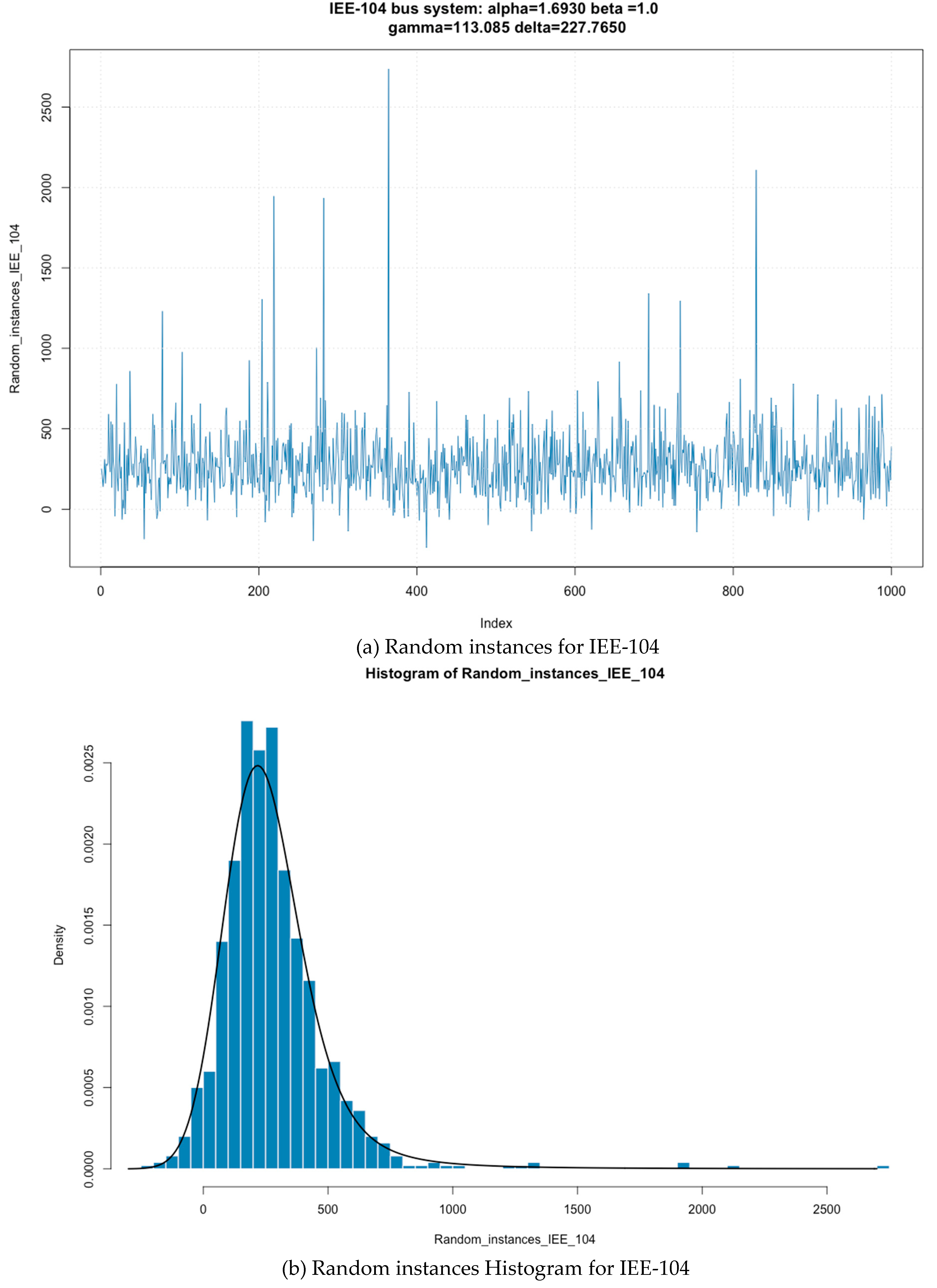
Figure 2 shows the simulation of random instances based on the IEEE-104 bus system with the alpha stable parameters $S(\alpha =1.6,\beta =1.0,\gamma =113.3,\delta =227.7)$ and the histogram of these instances. The presence of extreme values is observed as well as heavy tails in the distribution of the generated data. This system is the one with the greatest impulsiveness and dispersion in the data.

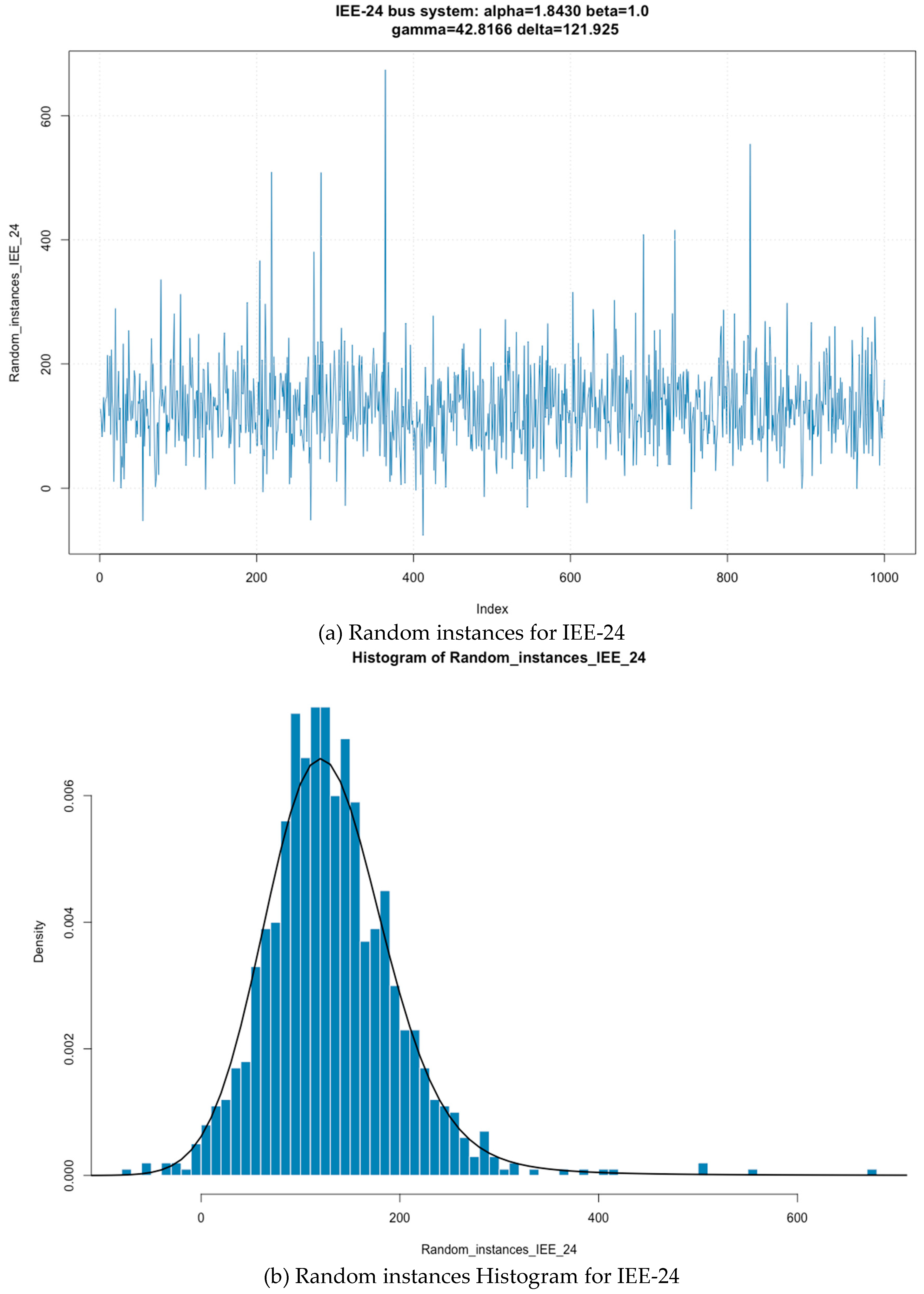
Figure 3 shows the simulation of instances based on the IEEE-24 bus system, with the alpha stable parameters $S(\alpha =1.8,\beta =1.0,\gamma =42.8,\delta =121.9)$ and the histogram of these instances. Given the characteristics of the system, the demand peaks are observed. The estimated distribution parameters show the dispersion in each system through the delta parameter and the impulsivity through the alpha parameter. This system, given the value of alpha, is the closest to a behavior of a Gaussian distribution $(\alpha =2)$.

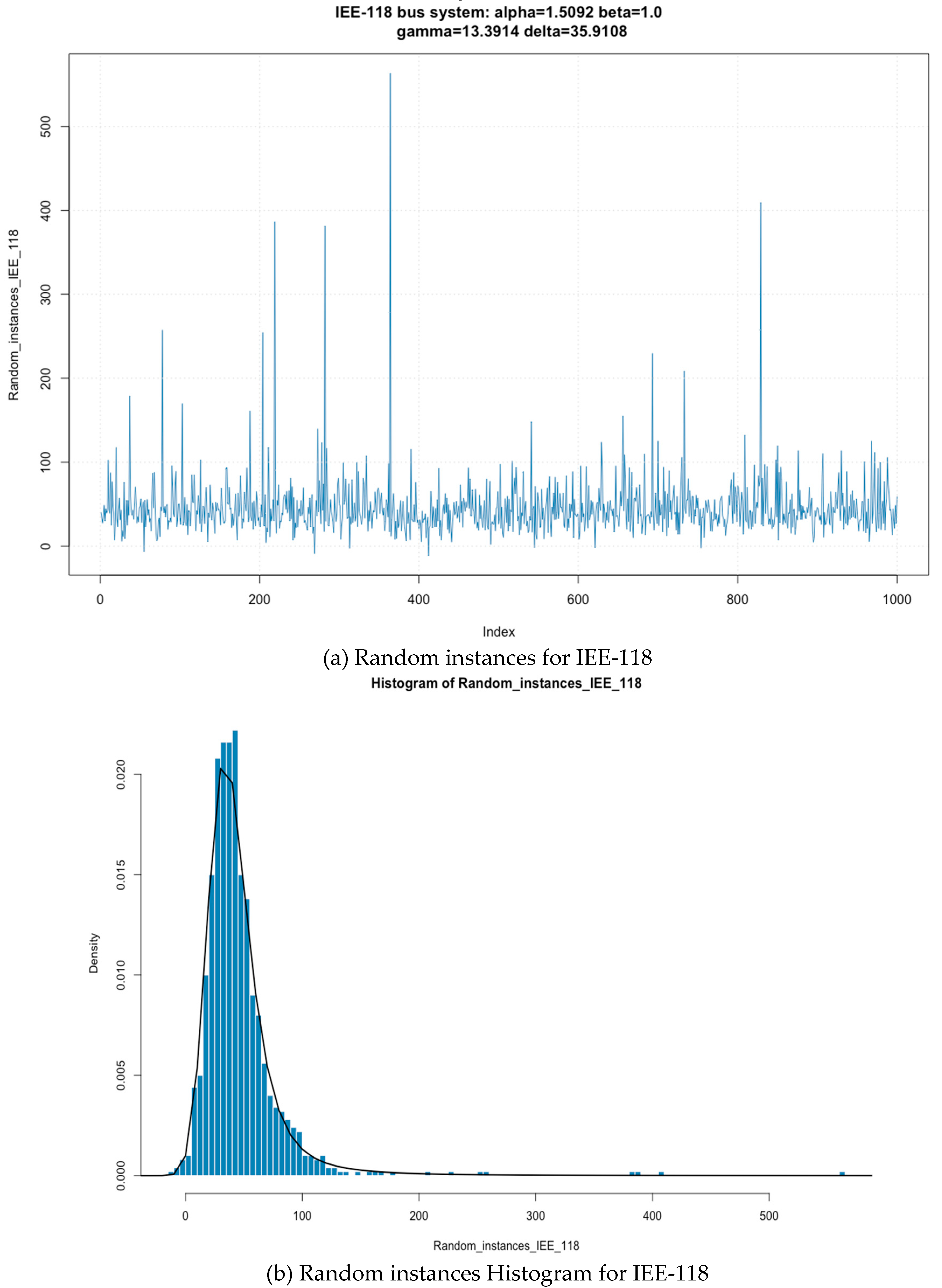
Figure 4 shows the simulation of instances based on the IEEE-118 bus system, with the alpha stable parameters $S(\alpha =1.5,\beta =1.0,\gamma =13.9,\delta =35.9)$ and the histogram of these instances. This system shows impulsiveness and significant dispersion.

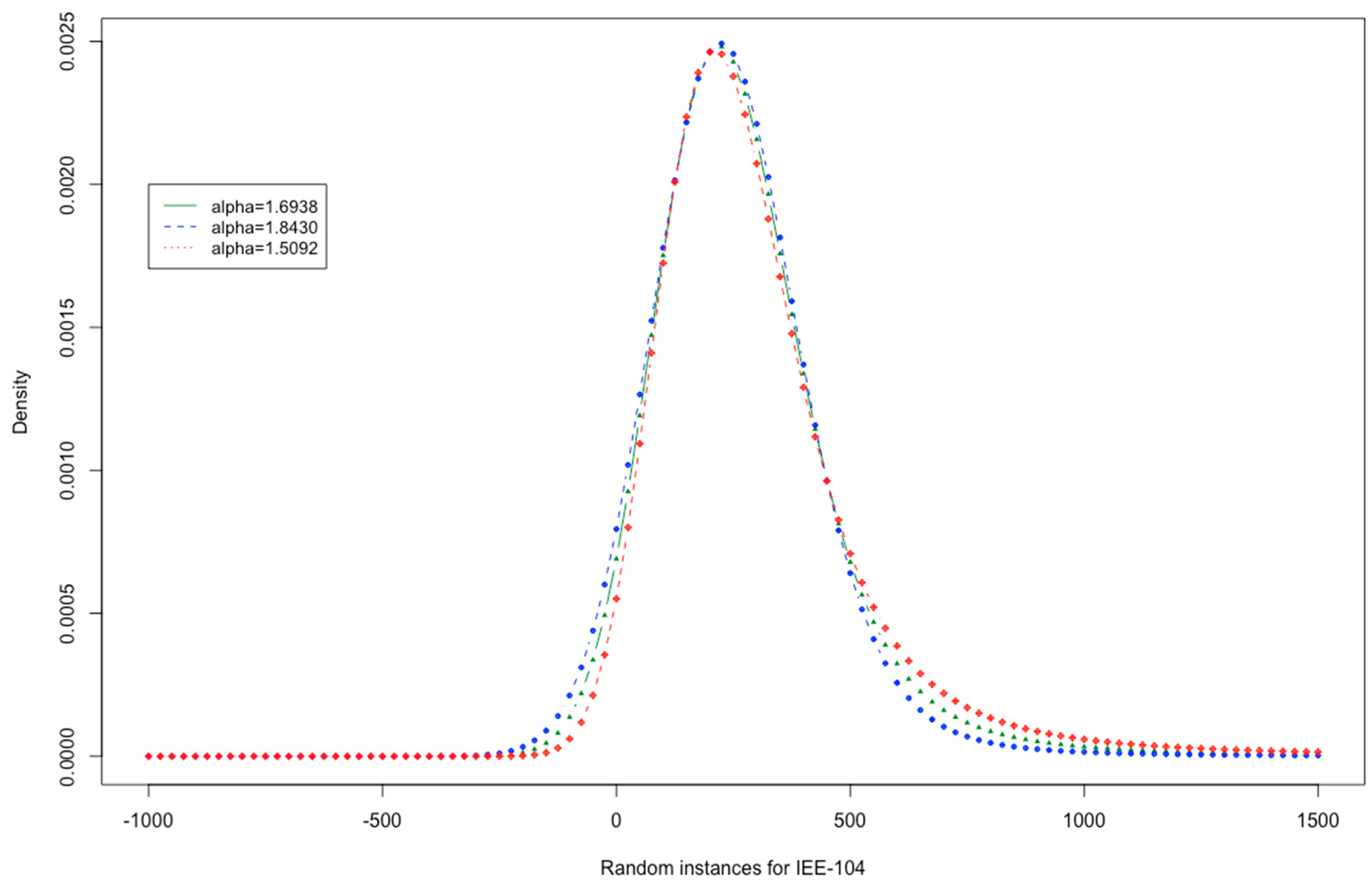
The fitting of the data to the stable distribution and the generation of instances, according to the parameters, show the presence of heavy tails and impulsivity in the generated data. The alpha parameter measures the impulsivity of the series and defines how heavy are the tails of the distribution of probability. Figure 5 shows different scenarios of impulsivity parameter generating differences in the tails of the distribution of the IEE-104 simulated system. The example of this system was used since it was the one with the most impulsiveness.

It is relevant to know the effect of the alpha parameter on the impulsivity of the series. The impulsivity of the series differs depending on the architecture of the system. Therefore, having parameters from different systems will allow us to generate extreme scenarios to evaluate in the optimization model used. Once the stable alpha random values for the energy demand per test system have been generated, it is necessary to consider the seasonal effect of the demand. For this, the estimation of a GAM will be carried out using spline functions. This will be made using the previously generated random demand data as inputs so that there will be enough data to make the right fit.

4.2. Generalized Additive Model (GAM)

Using the information of simulated data through the alpha stable distribution, the estimation of a generalized additive model was carried out, which will take as a dependent variable the demand for electric energy, and as explanatory variables, the price of energy (local marginal price) and fuel prices (fuel oil) for a sample of data is used with weekly data for 52 weeks [49]. The model estimated is presented in Equation (26):

$$X_i={\theta }_0+S_1(LM{P}_i)+S_2(PCOM{B}_i)+{\epsilon }_i,i=1,\dots ,$$

(26)

where

• $X_i$ is the demand for the period $i$.
• $LM{P}_i$ is the Local Marginal Price for the period $i$.
• $PCOM{B}_i$ is Fuel Oil Price for the period $i$.
• $S_j$ are smoothing splines functions for each parameter, $j=1, 2.$

The results of the GAM model show that smoothing splines are statistically significant for non-parametric estimates, so there are non-linear relationships between the variables associated with these functions and the dependent variable.

Table 2. Generalized additive model (GAM) parameter estimations.

ANOVA for Parametric Effects	Df	F-Value	Pr (>F)	Parameter
S(LMP)	1	57.4724	0.00000
S(PCOMB)	1	2.4594	0.12330
Residuals	49
ANOVA for Nonparametric Effects	NPar Df	Npar F	Pr (F)
Intercept				4320.1975
S(LMP)	3	3.6108	0.01958	0.3957
S(PCOMB)	3	9.3544	0.00005	2.9405

Null deviance: 13,492,752 on 57 degrees of freedom. Residual deviance: 3,607,220 on 49.0003 degrees of freedom. AIC: 824.8005.

shows the estimated parameters for the generalized additive model, which uses demand as a dependent variable, a variable that is constructed through the simulation of instances based on the three base systems used (IEEE-104, IEEE-24, and IEEE-18) and the sample of data on LMP and fuel prices (PCOMB) for 52 weeks.

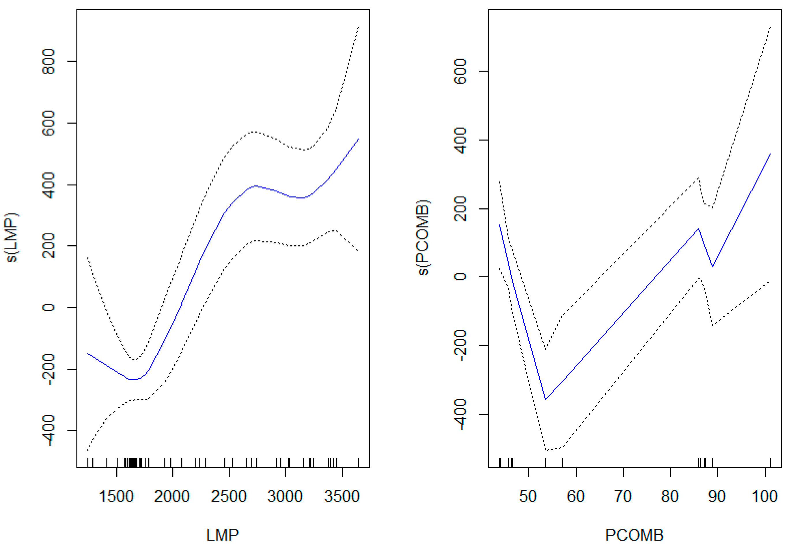
The benefit of using GAM models is that the non-linear effect of each independent variable can be modeled separately, keeping the rest constant and assessing the additive effect of all explanatory variables and can include as many explanatory variables as want to evaluate. Figure 6 shows the non-linear relationship fitted by the smoothing spline function in the estimated additive model for LMP and PCOMB variables.

The estimates with the proposed generalized additive model show an adequate fit to the observed behavior of the demand for electrical energy. To compare the results of the non-linear fit of the behavior of the demand for electrical energy, the coefficient of determination was estimated $(R^2=1-\frac{SSE}{SST})$. In addition, three non-linear models were compared: (a) GAM, (b) local regression, and (c) polynomial regression. 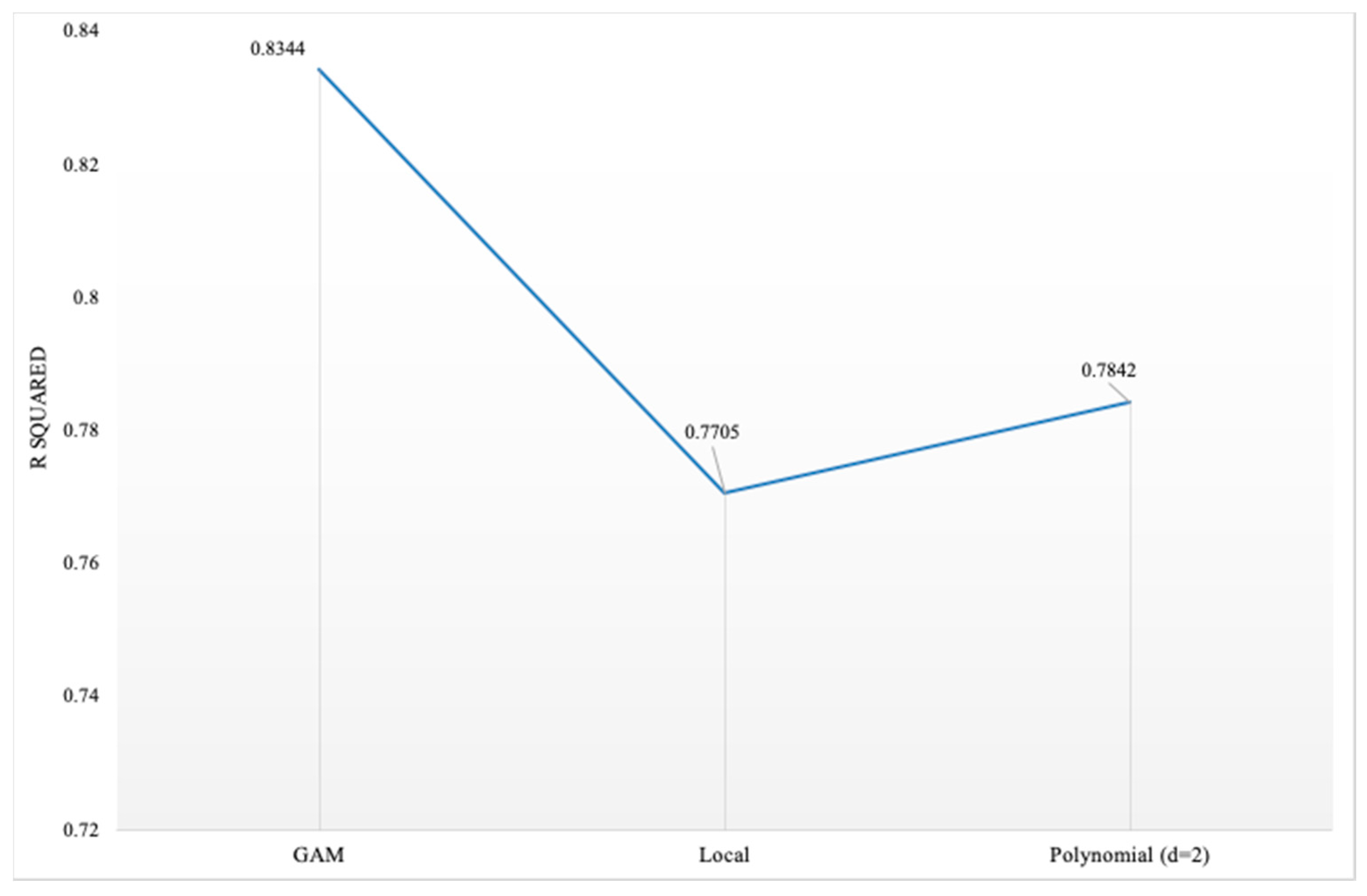Figure 7 shows the coefficient of determination $(R^2)$ for the three compared non-linear fitting methods.

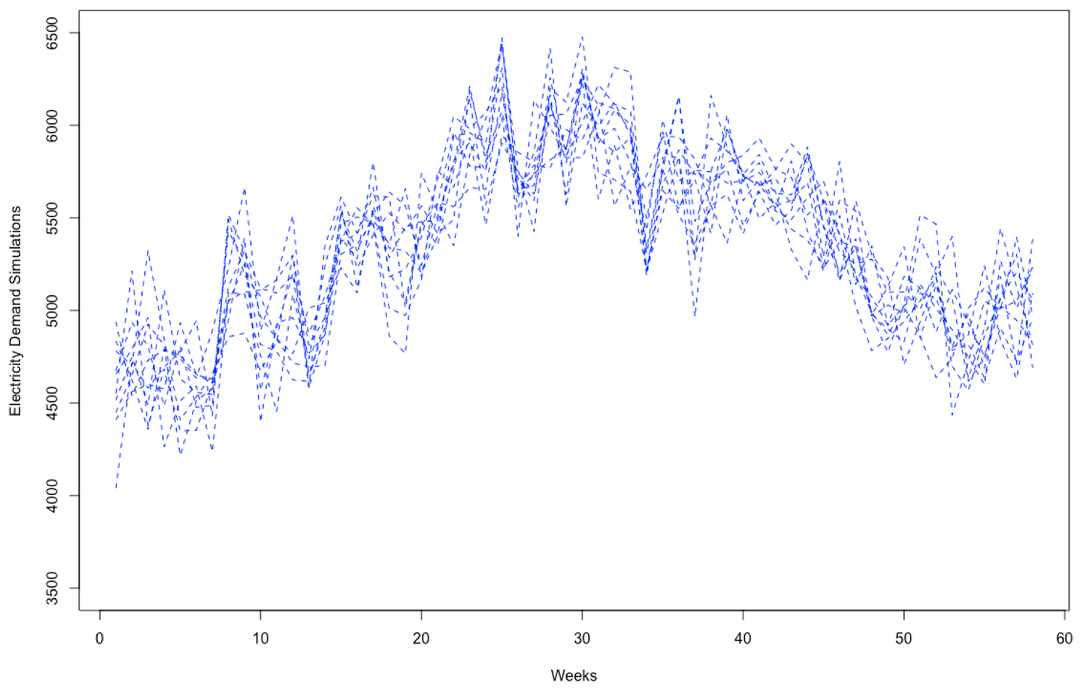
The results of the coefficient of determination show that while the local regression model and the polynomial model share a similar $R^2$, the GAM model shows the best result $(R^2=0.8344)$. With GAM fitted, it is possible to simulate complete periods of demand for the test cases. Figure 8 shows 10 simulations (only 10 for graphic reasons) of the cases. It can be seen that when simulating the data with the final GAM fitted, seasonal behavior is maintained as well as peaks in demand.

The methodological proposal shows that by combining the simulation of alpha stable variables and fitting a generalized additive model, it is possible to generate as many cases data as is required for an electrical system. This generation of unlimited test cases is an input of great importance for stress analysis for algorithms for solving the economic dispatch problem, further maintaining the presence of extreme values, as well as the seasonality of demand.

4.3. Comparison between the Hybrid Model and the Simulation of Normal Random Variables

The application of optimization algorithms to solve the economic dispatch problem requires test cases to evaluate the stability and quality of the solution found. An electrical reference system is used to test the algorithms, and the economic dispatch problem is solved based on historical information [12,13,14,15,16].

Given the requirement of enough test cases, information for the validation of optimization algorithms, a widely used option is the simulation of demand data generating random values assuming a normal probability distribution. One of the main limitations of this method is that generated values are limited to the parameters of a normal distribution, their mean, and standard deviation $N~(\mu , {\sigma }^2)$. Since it is documented that the demand for electrical energy presents heavy tails in its distribution, further seasonality related to the time of day, day of the week, and month of the year analyzed [22,23,24,25,26,27,28].

The proposed methodology addresses these aspects through the hybrid model that fitting of the electricity demand through the use of alpha stable distributions coupled with the modeling of seasonality and non-linear behavior through the use of GAM by integrating additive non-linear functions, such as spline functions or kernel functions, to variables such as the price of electrical energy, as well as the cost of the fuels, among others. 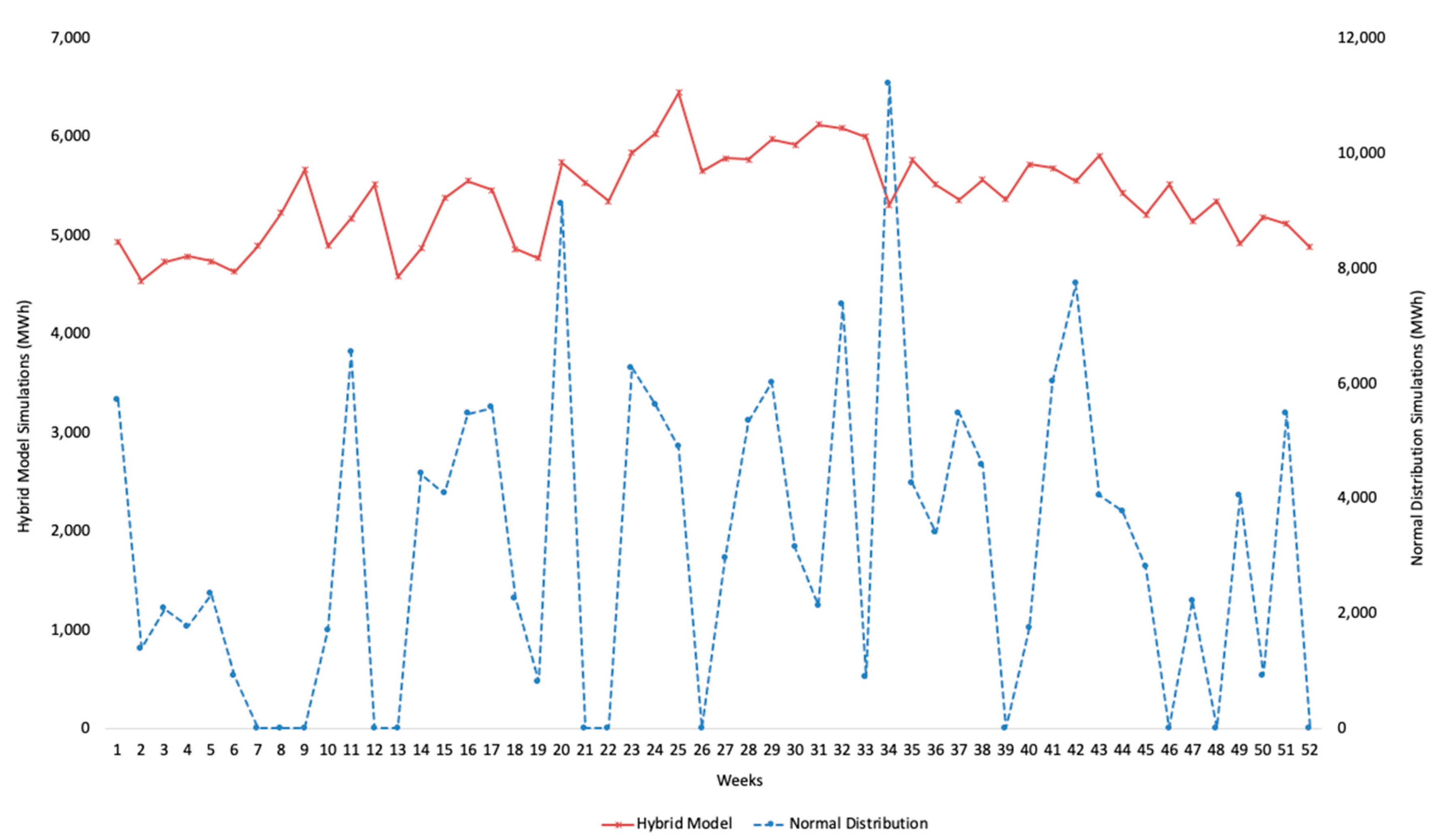Figure 9 shows the comparison between the simulation of normal random demands to simulated demands using the proposed hybrid model for a period of 52 weeks.

It is observed that the generation of instances only using normal random numbers generates demands without any seasonal pattern besides presenting abrupt variations in demand, which are just random. Also, it is necessary to limit the generated values to only positive values, so that when the negative values of the distribution are generated, they take the value of zero. On the other hand, in the case of the hybrid model, the presence of peaks in demand, as well as seasonality, is observed. This lets generating instances more attached to reality and therefore subjecting the optimization models to more realistic demands. Thus, contributing to generate more stable and higher quality models, tested in real-life scenarios.

5. Discussion and Conclusions

The problem of economic dispatch is a classic problem in the planning of the generation and expansion of electricity networks. There are multiple representations of the problem according to its objectives, including the inclusion of renewable energy, the emissions generated as well as restrictions on fuel availability, among many other nuances. Similarly, the method of solving the problem has had various approaches to achieve more efficient solutions. To be able to test the algorithms for solving the problem of economic dispatch, it is necessary to have a large amount of test data information, which reflects the real behavior of the electricity grid and permits the consideration of stress scenarios. There are some approaches in this regard in the literature; however, the proposals are limited to the representation of reference architectures and the availability of historical data for specific networks.

It has been documented that the demand for electricity has a particular behavior, with peak demand and seasonal effects during the day and during the year. The objective of the hybrid model using alpha stable distribution is to admit the simulation of demand peaks and seasonality. This lets us simulate demand data in specific time intervals according to the objective of planning or solution required for the problem of economic dispatch.

This work covers a conceptual framework that includes the use of predefined architectures and historical data, consolidating the unlimited generation of test data and stress scenarios through the application of alpha stable distributions and generalized additive models. The proposal contemplates the generation of as many test cases as necessary for the validation of the optimization algorithms, as well as consenting exposure to stress scenarios. The results of the application of the model show the generation of test cases for long periods that maintain the seasonality and impulsivity of demand. The combination of heavy tail distributions and generalized additive models presents a better fit, as well as unlimited test case generation.

The proposed model integrates three stages of analysis: (1) collection of historical information of specific network architecture, (2) fitting of the alpha stable distribution to be able to simulate as much data as necessary, and (3) estimation of a generalized additive model to fit test data required, according to a specific time interval capturing the seasonality and non-linearity. These generated data will be the input used to test the optimization algorithms for the economic dispatch problem posed.

According to the data used in the case study, it is shown that the demand data for electrical energy show impulsivity and heavy tails that are consistent with the presence of demand peaks. Similarly, the fitting of the GAM model shows that the energy demand has a non-linear behavior, so the use of an additive model is a good alternative to have a better fit to the data. The use of smoothing splines functions showed a good fit to the data.

One of the main advantages of the proposal is that it is possible to use information from different available electrical networks and thereby check the efficiency of the optimization algorithms for different scenarios and not only for a particular case. This will strengthen the proposed solutions and contemplate real-life cases.