Implementing AutoML in Educational Data Mining for Prediction Tasks


Abstract
1. Introduction
2. Related Work
2.1. Related Work on Predicting Student Academic Performance
2.2. Related Work on Predicting Student Grade
2.3. Related Work on Predicting Student Dropout
3. Introduction to Bayesian Optimization for Hyperparameter Optimization
3.1. Definitions
3.2. Bayesian Optimization
| Algorithm 1: The sequential model-based optimization algorithm |
| Input: , Output: from with minimal
|
3.3. Use Cases
4. Method
4.1. Research Goal
4.2. Procedure
4.3. Data Collection
4.4. Data Analysis
4.5. Feature Importance
4.6. Evaluation Measures
4.7. Environment
4.8. ML Algorithms
- Bayes classifiers: Based on the Bayes theorem, the Bayes classifiers constitute a simple approach that often achieves impressive results. Naïve Bayes is a well-known probabilistic induction method [72].
- Rule-based classifiers: In general, rule-based classifiers classify records by using a collection of “if … then …” rules. PART uses separate-and-conquer. In each iteration the algorithm builds a partial C4.5 decision tree and makes the “best” leaf into a rule [73]. M5Rules is a rule learning algorithm for regression problems. It builds a model tree using M5 and makes the “best” leaf into a rule [74].
- Tree-based classifiers: Tree-based classifiers is another approach to the problem of learning. An example is Random Forest classifier that generates a large number of random trees (i.e., forest) and uses the majority voting to classify a new instance [75].
- Lazy classifiers: Lazy learners do not train a specific model. At the prediction time, they evaluate an unknown instance based on the most related instances stored as training data. IBk is the k-nearest neighbor’s classifier that is able to analyze the closest k number of training instances (nearest neighbors) and returns the most common class or the mean of k nearest neighbors for the classification and regression task respectively [81].
- Meta classifiers: Meta classifiers either enhance a single classifier or combine several classifiers. Bagging predictors is a method for generating multiple versions of a predictor and using them in order to get an aggregated predictor [82].
5. Results
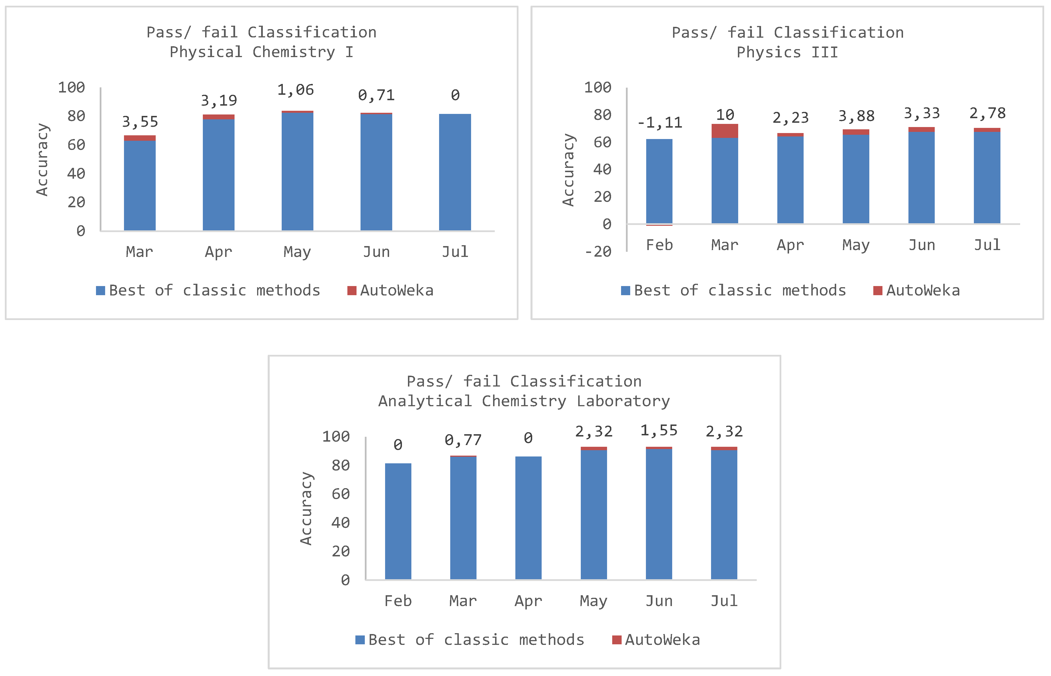
5.1. Predicting Pass/Fail Students
5.2. Predicting Students’ Academic Performance
5.3. Predicting Dropout Students
6. Discussion
7. Conclusions and Future Research Directions
Author Contributions
Funding
Conflicts of Interest
References
- Romero, C.; Ventura, S. Data mining in education. Wiley Interdiscip. Rev. Data Min. Knowl. Discov. 2013, 3, 12–27. [Google Scholar] [CrossRef]
- Bakhshinategh, B.; Zaiane, O.R.; ElAtia, S.; Ipperciel, D. Educational data mining applications and tasks: A survey of the last 10 years. Educ. Inf. Technol. 2018, 23, 537–553. [Google Scholar] [CrossRef]
- Romero, C.; Ventura, S. Educational data mining: A review of the state of the art. IEEE Trans. Syst. Man Cybern. Part C Appl. Rev. 2010, 40, 601–618. [Google Scholar] [CrossRef]
- Bousbia, N.; Belamri, I. Which Contribution Does EDM Provide to Computer-Based Learning Environments? In Educational Data Mining; Springer: Basel, Switzerland, 2014; pp. 3–28. [Google Scholar]
- Romero, C.; Ventura, S. Educational data science in massive open online courses. Wiley Interdiscip. Rev. Data Min. Knowl. Discov. 2017, 7, e1187. [Google Scholar] [CrossRef]
- Wolff, A.; Zdrahal, Z.; Herrmannova, D.; Knoth, P. Predicting student performance from combined data sources. In Educational Data Mining; Springer: Basel, Switzerland, 2014; pp. 175–202. [Google Scholar]
- Campbell, J.P.; DeBlois, P.B.; Oblinger, D.G. Academic analytics: A new tool for a new era. Educ. Rev. 2007, 42, 40–57. [Google Scholar]
- Romero, C.; Ventura, S. Educational data mining: A survey from 1995 to 2005. Expert Syst. Appl. 2007, 33, 135–146. [Google Scholar] [CrossRef]
- Daniel, B. Big Data and analytics in higher education: Opportunities and challenges. Br. J. Educ. Technol. 2015, 46, 904–920. [Google Scholar] [CrossRef]
- Bergstra, J.S.; Bardenet, R.; Bengio, Y.; Kégl, B. Algorithms for hyper-parameter optimization. In Advances in Neural Information Processing Systems; Curran Associates Inc.: New York, NY, USA, 2011. [Google Scholar]
- Snoek, J.; Larochelle, H.; Adams, R.P. Practical bayesian optimization of machine learning algorithms. In NIPS’12 Proceedings of the 25th International Conference on Neural Information Processing Systems; Curran Associates Inc.: New York, NY, USA, 2012. [Google Scholar]
- Thornton, C.; Hutter, F.; Hoos, H.H.; Leyton-Brown, K. Auto-WEKA: Combined selection and hyperparameter optimization of classification algorithms. In Proceedings of the 19th ACM SIGKDD International Conference on Knowledge Discovery and Data Mining, Chicago, IL, USA, 11–14 August 2013. [Google Scholar]
- Bergstra, J.; Yamins, D.; Cox, D.D. Hyperopt: A python library for optimizing the hyperparameters of machine learning algorithms. In Proceedings of the 12th Python in Science Conference, Brussels, Belgium, 21–25 August 2013. [Google Scholar]
- Galitsky, B. Customers’ Retention Requires an Explainability Feature in Machine Learning Systems They Use. In Proceedings of the 2018 AAAI Spring Symposium Series, Palo Alto, CA, USA, 26–28 March 2018. [Google Scholar]
- Martens, D.; Vanthienen, J.; Verbeke, W.; Baesens, B. Performance of classification models from a user perspective. Decis. Support Syst. 2011, 51, 782–793. [Google Scholar] [CrossRef]
- Došilović, F.K.; Brčić, M.; Hlupić, N. Explainable artificial intelligence: A survey. In 2018 41st International Convention on Information and Communication Technology, Electronics and Microelectronics (MIPRO); IEEE: Opatija, Croatia, 2018. [Google Scholar]
- Hämäläinen, W.; Vinni, M. Classifiers for educational data mining. In Handbook of Educational Data Mining; CRC Press: Boca Raton, FL, USA, 2010; pp. 57–74. [Google Scholar]
- Conijn, R.; Snijders, C.; Kleingeld, A.; Matzat, U. Predicting student performance from LMS data: A comparison of 17 blended courses using Moodle LMS. IEEE Trans. Learn. Technol. 2016, 10, 17–29. [Google Scholar] [CrossRef]
- Márquez-Vera, C.; Cano, A.; Romero, C.; Ventura, S. Predicting student failure at school using genetic programming and different data mining approaches with high dimensional and imbalanced data. Appl. Intell. 2013, 38, 315–330. [Google Scholar] [CrossRef]
- Moreno-Marcos, P.M.; Alario-Hoyos, C.; Muñoz-Merino, P.J.; Kloos, C.D. Prediction in MOOCs: A review and future research directions. IEEE Trans. Learn. Technol. 2018, 12. [Google Scholar] [CrossRef]
- Mueen, A.; Zafar, B.; Manzoor, U. Modeling and predicting students’ academic performance using data mining techniques. Int. J. Mod. Educ. Comput. Sci. 2016, 8, 36–42. [Google Scholar] [CrossRef]
- Amrieh, E.A.; Hamtini, T.; Aljarah, I. Mining educational data to predict student’s academic performance using ensemble methods. Int. J. Database Theory Appl. 2016, 9, 119–136. [Google Scholar] [CrossRef]
- Kaur, P.; Singh, M.; Josan, G.S. Classification and prediction based data mining algorithms to predict slow learners in education sector. Procedia Comput. Sci. 2015, 57, 500–508. [Google Scholar] [CrossRef]
- Guo, B.; Zhang, R.; Xu, G.; Shi, C.; Yang, L. Predicting students performance in educational data mining. In Proceedings of the 2015 International Symposium on Educational Technology (ISET), Wuhan, China, 27–29 July 2015. [Google Scholar]
- Saa, A.A. Educational data mining & students’ performance prediction. Int. J. Adv. Comput. Sci. Appl. 2016, 7, 212–220. [Google Scholar]
- Costa, E.B.; Fonseca, B.; Santana, M.A.; de Araújo, F.F.; Rego, J. Evaluating the effectiveness of educational data mining techniques for early prediction of students’ academic failure in introductory programming courses. Comput. Hum. Behav. 2017, 73, 247–256. [Google Scholar] [CrossRef]
- Asif, R.; Merceron, A.; Ali, S.A.; Haider, N.G. Analyzing undergraduate students’ performance using educational data mining. Comput. Educ. 2017, 113, 177–194. [Google Scholar] [CrossRef]
- Kostopoulos, G.; Kotsiantis, S.; Pintelas, P. Predicting student performance in distance higher education using semi-supervised techniques. In Model and Data Engineering; Springer: New York, NY, USA, 2015; pp. 259–270. [Google Scholar]
- Elbadrawy, A.; Polyzou, A.; Ren, Z.; Sweeney, M.; Karypis, G.; Rangwala, H. Predicting student performance using personalized analytics. Computer 2016, 49, 61–69. [Google Scholar] [CrossRef]
- Xu, J.; Moon, K.H.; van der Schaar, M. A machine learning approach for tracking and predicting student performance in degree programs. IEEE J. Sel. Top. Signal Process. 2017, 11, 742–753. [Google Scholar] [CrossRef]
- Strecht, P.; Cruz, L.; Soares, C.; Mendes-Moreira, J.; Abreu, R. A Comparative Study of Classification and Regression Algorithms for Modelling Students’ Academic Performance. In Proceedings of the 8th International Conference on Educational Data Mining, Madrid, Spain, 26–29 June 2015. [Google Scholar]
- Meier, Y.; Xu, J.; Atan, O.; van der Schaar, M. Personalized grade prediction: A data mining approach. In Proceedings of the 2015 IEEE International Conference on Data Mining, Atlantic City, NJ, USA, 14–17 November 2015. [Google Scholar]
- Sweeney, M.; Rangwala, H.; Lester, J.; Johri, A. Next-term student performance prediction: A recommender systems approach. arXiv 2016, arXiv:1604.01840. [Google Scholar]
- Kostopoulos, G.; Kotsiantis, S.; Fazakis, N.; Koutsonikos, G.; Pierrakeas, C. A Semi-Supervised Regression Algorithm for Grade Prediction of Students in Distance Learning Courses. Int. J. Artif. Intell. Tools 2019, 28, 1940001. [Google Scholar] [CrossRef]
- Tsiakmaki, M.; Kostopoulos, G.; Koutsonikos, G.; Pierrakeas, C.; Kotsiantis, S.; Ragos, O. Predicting University Students’ Grades Based on Previous Academic Achievements. In Proceedings of the 2018 9th International Conference on Information, Intelligence, Systems and Applications (IISA), Zakynthos, Greece, 23–25 July 2018. [Google Scholar]
- Márquez-Vera, C.; Cano, A.; Romero, C.; Noaman, A.Y.M.; Fardoun, H.M.; Ventura, S. Early dropout prediction using data mining: A case study with high school students. Expert Syst. 2016, 33, 107–124. [Google Scholar] [CrossRef]
- Zhang, Y.; Oussena, S.; Clark, T.; Kim, H. Use Data Mining to Improve Student Retention in Higher Education-A Case Study. In Proceedings of the 12th International Conference on Enterprise Information Systems, Volume 1, DISI, Funchal, Madeira, Portugal, 8–12 June 2010. [Google Scholar]
- Delen, D. A comparative analysis of machine learning techniques for student retention management. Decis. Support Syst. 2010, 49, 498–506. [Google Scholar] [CrossRef]
- Lykourentzou, I.; Giannoukos, I.; Nikolopoulos, V.; Mpardis, G.; Loumos, V. Dropout prediction in e-learning courses through the combination of machine learning techniques. Comput. Educ. 2009, 53, 950–965. [Google Scholar] [CrossRef]
- Superby, J.-F.; Vandamme, J.P.; Meskens, N. Determination of factors influencing the achievement of the first-year university students using data mining methods. In Proceedings of the Workshop on Educational Data Mining, Jhongli, Taiwan, 26–30 June 2006. [Google Scholar]
- Herzog, S. Estimating student retention and degree-completion time: Decision trees and neural networks vis-à-vis regression. New Dir. Inst. Res. 2006, 2006, 17–33. [Google Scholar] [CrossRef]
- Kostopoulos, G.; Kotsiantis, S.; Pintelas, P. Estimating student dropout in distance higher education using semi-supervised techniques. In Proceedings of the 19th Panhellenic Conference on Informatics, Athens, Greece, 1–3 October 2015. [Google Scholar]
- Rao, S.S. Engineering Optimization: Theory and Practice; John Wiley & Sons: Toronto, ON, Canada, 2009. [Google Scholar]
- Brochu, E. Interactive Bayesian Optimization: Learning User Preferences for Graphics and Animation; University of British Columbia: Vancouver, BC, Canada, 2010. [Google Scholar]
- Feurer, M.; Hutter, F. Hyperparameter Optimization. In Automated Machine Learning: Methods, Systems, Challenges; Springer: New York, NY, USA, 2019; pp. 3–33. [Google Scholar]
- Brochu, E.; Cora, V.M.; de Freitas, N. A tutorial on Bayesian optimization of expensive cost functions, with application to active user modeling and hierarchical reinforcement learning. arXiv 2010, arXiv:1012.2599. [Google Scholar]
- Hutter, F.; Kotthoff, L.; Vanschoren, J. Automated Machine Learning-Methods, Systems, Challenges; Springer: New York, NY, USA, 2019. [Google Scholar]
- Bergstra, J.; Bengio, Y. Random search for hyper-parameter optimization. J. Mach. Learn. Res. 2012, 13, 281–305. [Google Scholar]
- Bengio, Y. Gradient-based optimization of hyperparameters. Neural Comput. 2000, 12, 1889–1900. [Google Scholar] [CrossRef]
- Maron, O.; Moore, A.W. The racing algorithm: Model selection for lazy learners. Artif. Intell. Rev. 1997, 11, 193–225. [Google Scholar] [CrossRef]
- Simon, D. Evolutionary Optimization Algorithms; Wiley: Hoboken, NJ, USA, 2013. [Google Scholar]
- Guo, X.C.; Yang, J.H.; Wu, C.G.; Wang, C.Y.; Liang, Y.C. A novel LS-SVMs hyper-parameter selection based on particle swarm optimization. Neurocomputing 2008, 71, 3211–3215. [Google Scholar] [CrossRef]
- Dewancker, I.; McCourt, M.; Clark, S. Bayesian Optimization Primer; SigOpt. 2015. Available online: https://app.sigopt.com/static/pdf/SigOpt_Bayesian_Optimization_Primer.pdf (accessed on 12 June 2019).
- Hutter, F.; Lücke, J.; Schmidt-Thieme, L. Beyond manual tuning of hyperparameters. Künstliche Intell. 2015, 29, 329–337. [Google Scholar] [CrossRef]
- Shahriari, B.; Swersky, K.; Wang, Z.; Adams, R.P.; de Freitas, N. Taking the human out of the loop: A review of bayesian optimization. Proc. IEEE 2016, 104, 148–175. [Google Scholar] [CrossRef]
- Williams, C.K.I.; Rasmussen, C.E. Gaussian Processes for Machine Learning; MIT Press: Cambridge, MA, USA, 2006; Volume 2. [Google Scholar]
- Bergstra, J.; Yamins, D.; Cox, D.D. Making a Science of Model Search: Hyperparameter Optimization in Hundreds of Dimensions for Vision Architectures. In Proceedings of the 30th International Conference on International Conference on Machine Learning, Atlanta, GA, USA, 16–21 June 2013. [Google Scholar]
- Breiman, L.; Friedman, J.; Olshen, R.; Stone, C. Classification and Regression Trees; Wadsworth Int. Group: Belmont, CA, USA, 1984; Volume 37, pp. 237–251. [Google Scholar]
- Hutter, F.; Hoos, H.H.; Leyton-Brown, K. Sequential model-based optimization for general algorithm configuration. In Proceedings of the International Conference on Learning and Intelligent Optimization, Rome, Italy, 17–21 January 2011. [Google Scholar]
- Eggensperger, K.; Feurer, M.; Hutter, F.; Bergstra, J.; Snoek, J.; Hoos, H.; Leyton-Brown, K. Towards an empirical foundation for assessing bayesian optimization of hyperparameters. In Proceedings of the NIPS Workshop on Bayesian Optimization in Theory and Practice, Lake Tahoe, NV, USA, 10 December 2013. [Google Scholar]
- Jones, D.R.; Schonlau, M.; Welch, W.J. Efficient global optimization of expensive black-box functions. J. Glob. Optim. 1998, 13, 455–492. [Google Scholar] [CrossRef]
- Kushner, H.J. A new method of locating the maximum point of an arbitrary multipeak curve in the presence of noise. J. Basic Eng. 1964, 86, 97–106. [Google Scholar] [CrossRef]
- Srinivas, N.; Krause, A.; Kakade, S.M.; Seeger, M. Gaussian process optimization in the bandit setting: No regret and experimental design. arXiv 2009, arXiv:0912.3995. [Google Scholar]
- Clark, S.; Liu, E.; Frazier, P.; Wang, J.; Oktay, D.; Vesdapunt, N. MOE: A Global, Black Box Optimization Engine for Real World Metric Optimization. 2014. Available online: https://github.com/Yelp/MOE (accessed on 12 June 2019).
- Geurts, P.; Ernst, D.; Wehenkel, L. Extremely randomized trees. Mach. Learn. 2006, 63, 3–42. [Google Scholar] [CrossRef]
- Jeni, L.A.; Cohn, J.F.; de la Torre, F. Facing imbalanced data–recommendations for the use of performance metrics. In Proceedings of the 2013 Humaine Association Conference on Affective Computing and Intelligent Interaction, Geneva, Switzerland, 2–5 September 2013. [Google Scholar]
- Ling, C.X.; Huang, J.; Zhang, H. AUC: A better measure than accuracy in comparing learning algorithms. In Proceedings of the Conference of the Canadian Society for Computational Studies of Intelligence, Halifax, NS, Canada, 11–13 June 2003. [Google Scholar]
- Provost, F.; Fawcett, T. Analysis and Visualization of Classifier Performance: Comparison under Imprecise Class and Cost Distributions. In Proceedings of the Third International Conference on Knowledge Discovery and Data Mining, Newport Beach, CA, USA, 14–17 August 1997. [Google Scholar]
- Frank, E.; Hall, M.A.; Witten, I.H. The WEKA Workbench. Online Appendix for Data Mining: Practical Machine Learning Tools and Techniques, 4th ed.; Morgan Kaufmann: Massachusetts, MA, USA, 2016. [Google Scholar]
- Kotthoff, L.; Thornton, C.; Hoos, H.H.; Hutter, F.; Leyton-Brown, K. Auto-WEKA 2.0: Automatic model selection and hyperparameter optimization in WEKA. J. Mach. Learn. Res. 2017, 18, 826–830. [Google Scholar]
- Witten, I.H.; Frank, E.; Hall, M.A.; Pal, C.J. Data Mining: Practical machine learning tools and techniques; Morgan Kaufmann: Massachusetts, MA, USA, 2016. [Google Scholar]
- John, G.H.; Langley, P. Estimating continuous distributions in Bayesian classifiers. In Proceedings of the Eleventh Conference on Uncertainty in Artificial Intelligence, Montreal, QC, Canada, 18–20 August 1995. [Google Scholar]
- Eibe, F.; Witten, I.H. Generating Accurate Rule Sets without Global Optimization; University of Waikato, Department of Computer Science: Hamilton, New Zealand, 1998. [Google Scholar]
- Holmes, G.; Hall, M.; Prank, E. Generating rule sets from model trees. In Proceedings of the Australasian Joint Conference on Artificial Intelligence, Sydney, Australia, 6–10 December 1999. [Google Scholar]
- Breiman, L. Random forests. Mach. Learn. 2001, 45, 5–32. [Google Scholar] [CrossRef]
- Platt, J. Fast Training of Support Vector Machines using Sequential Minimal Optimization. In Advances in Kernel Methods—Support Vector Learning; Schoelkopf, B., Burges, C., Smola, A., Eds.; MIT Press: Massachusetts, MA, USA, 1998. [Google Scholar]
- Keerthi, S.S.; Shevade, S.K.; Bhattacharyya, C.; Murthy, K.R.K. Improvements to Platt’s SMO Algorithm for SVM Classifier Design. Neural Comput. 2001, 13, 637–649. [Google Scholar] [CrossRef]
- Hastie, T.; Tibshirani, R. Classification by Pairwise Coupling. In Advances in Neural Information Processing Systems; MIT Press: Massachusetts, MA, USA, 1998. [Google Scholar]
- Shevade, S.K.; Keerthi, S.S.; Bhattacharyya, C.; Murthy, K.R.K. Improvements to the SMO Algorithm for SVM Regression. IEEE Transactions on Neural Netw. 2000, 11. [Google Scholar] [CrossRef]
- Smola, A.J.; Schoelkopf, B. A Tutorial on Support Vector Regression; Kluwer Academic Publishers: Dordrecht, The Netherlands, 1998. [Google Scholar]
- Aha, D.; Kibler, D. Instance-based learning algorithms. Mach. Learn. 1991, 6, 37–66. [Google Scholar] [CrossRef]
- Breiman, L. Bagging predictors. Mach. Learn. 1996, 24, 123–140. [Google Scholar] [CrossRef]
- Kim, B.-H.; Vizitei, E.; Ganapathi, V. GritNet: Student performance prediction with deep learning. arXiv 2018, arXiv:1804.07405. [Google Scholar]
- Caruana, R.; Niculescu-Mizil, A. An empirical comparison of supervised learning algorithms. In Proceedings of the 23rd International Conference on Machine Learning, Pittsburgh, PA, USA, 25–29 June 2006. [Google Scholar]
- Wolpert, D.H.; Macready, W.G. No free lunch theorems for optimization. IEEE Trans. Evol. Comput. 1997, 1, 67–82. [Google Scholar] [CrossRef]


| Paper | Prediction Task | Metrics | Methods Compared | Outperformers |
|---|---|---|---|---|
| Related work on predicting student academic performance | ||||
| [21] | Binary Classification | Accuracy, Precision, Recall, Specificity | NB, NNs, DTs | NB |
| [22] | Binary Classification | Accuracy, Precision, Recall, F-measure | ANN, NB, DTs, RF, Bagging, Boosting | ANN and Boosting |
| [23] | Binary Classification | Accuracy, Precision, Recall, F-measure, ROC Area | NB, MLPs, SMO, J48, REPTree | MLP |
| [24] | Multiclass Classification | Accuracy | NB, MLPs, SVM | Deep Neural Network |
| [25] | Multiclass Classification | Accuracy, Precision, Recall | C4.5, NB, ID3, CART, CHAID | CART |
| [26] | Binary Classification | F-measure | NNs, J48, SVM, NB | SVM fine-tuned |
| [27] | Multiclass Classification | Accuracy, Kappa | DTs, NB, NNs, Rule Induction, 1-NN, RF | NB |
| [28] | Binary Classification | Accuracy, Specificity | De-Tri-Training, Self-Training, Democratic, Tri-Training, Co-Training, RASCO, Rel-RASCO, C4.5 | Tri-Training (C4.5 as base learner) |
| Related work on predicting student grade | ||||
| [29] | Regression course grades | RMSE, MAE | Regression-based methods, Matrix factorization–based methods | Factorization machine |
| Assessments Grades | Depending on the records | |||
| [30] | Regression GPA | MAE | LR, LogR, RF, kNN | Proposed architecture |
| [31] | Regression course grades | RMSE | SVM, RF, AB.R2, kNN, OLS, CART | SVM |
| [32] | Regression course grades | Average absolute prediction error | Single performance assessment proposed architecture and Past Assessments, Weights, LR, 7-NN | Proposed architecture |
| [33] | Regression course grades | RMSE, MAE | Simple baselines, MF-based methods, regression models {RF, SGD, kNN, personalized LR} | Authors’ proposed hybrid model (FM-RF) |
| [34] | Regression course grades | MAE, RAE, RMSE, PCC | IBk, M5Rules, M5 Model Tree, LR, SMOreg, k-NN, RF, MSSRA | Proposed method (MSSRA) |
| [35] | Regression course grades | MAE | LR, RF, 5NN, M5 Rules, M5, SMOreg, GP, Bagging | RF, Bagging, SMOreg |
| Related work on predicting student dropout | ||||
| [36] | Classification (dropout) | Accuracy, TP rate, TN rate, GM | NB, SMO, IBk, JRip, J48, ICRM2 | Proposed architecture (ICRM2) |
| [37] | Classification (dropout) | Accuracy | NB, SVM, DTs | NB |
| [38] | Classification (dropout) | Accuracy | ANN, SVM DTS, LR, Information fusion, Bagging, Boosting | Information fusion |
| [39] | Classification (dropout) | Accuracy, Sensitivity, Precision | 3 decision schemes based on NN, SVM, and ARTMAP | Decision scheme 1 |
| [40] | Classification (dropout) | Accuracy | NNs, DTs, RF, Discriminant Analysis | NNs |
| [41] | Classification (dropout) | Accuracy | NNs, DTs, LR | DTs |
| [42] | Classification (dropout) | Accuracy, Sensitivity | Self-Training, Co-Training, Democratic Co-Training, Tri-Training, RASCO, Rel-RASCO, C4.5 | Tri-Training (C4.5) |
| Course | Female | Male | Total | Course Modules in Moodle |
|---|---|---|---|---|
| Physical Chemistry I | 122 | 160 | 282 | forum, resource, page, assign, folder |
| Physics III | 90 | 90 | 180 | forum, resource, page, assign |
| Analytical Chemistry Lab | 57 | 72 | 129 | forum, resource, page, assign, folder, URL |
| Total | 269 | 322 | 591 |
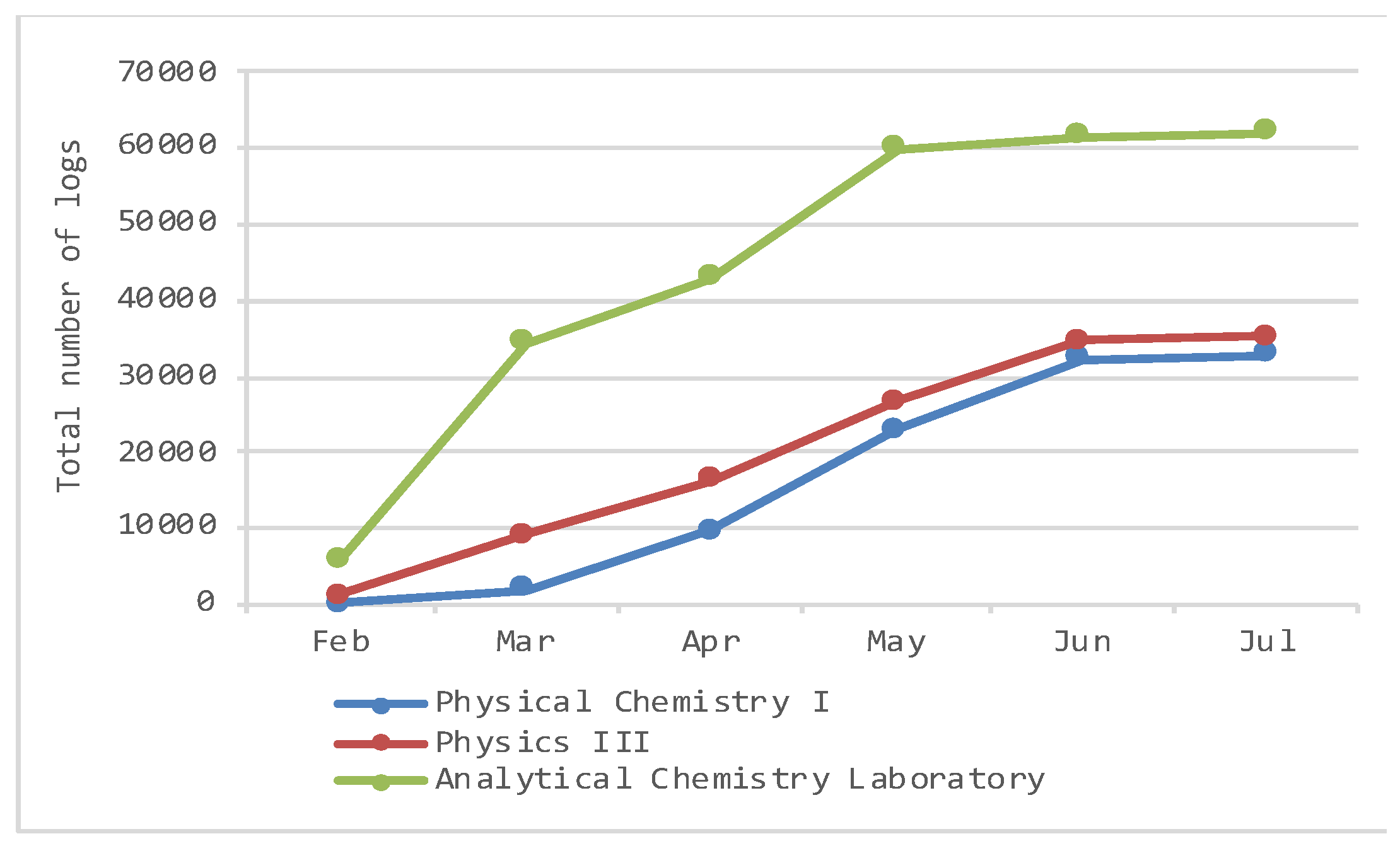
| February 2018 | March 2018 | April 2018 | May 2018 | June 2018 | July 2018 | |
|---|---|---|---|---|---|---|
| Physical Chemistry I | 0 | 2075 | 7617 | 13,175 | 9298 | 787 |
| 0 | 2075 | 9692 | 22,867 | 32,165 | 32,952 | |
| Physics III | 1156 | 8007 | 7259 | 10,369 | 7760 | 617 |
| 1156 | 9163 | 16,422 | 26,791 | 34,551 | 35,168 | |
| Analytical Chemistry Lab | 5800 | 28,564 | 8499 | 17,054 | 1623 | 416 |
| 5800 | 34,364 | 42,863 | 59,917 | 61,540 | 61,956 |
| Physical Chemistry I | Physics III | Analytical Chemistry Lab | Description | Possible Values |
|---|---|---|---|---|
| gender | gender | gender | Student’s gender | {female, male} |
| 1 forum 7 pages 17 resources 2 folders 8 assign views | 1 forum 6 pages 15 resources 9 assign views | 1 forum 2 pages 4 resources 17 folders 1 URL 8 assign views | Total number of times a student accessed the resource | 0 or positive integer |
| 3 assigns | 9 assigns | 8 assigns | Student grade | [0,10] |
| course total views | course total views | course total views | The total number of course views for an individual student | 0 or positive integer |
| course total activity | course total activity | course total activity | The total number of every kind of log written for an individual student | 0 or positive integer |
| 42 attributes | 44 attributes | 45 attributes |
| Regression | Classification | Classification | ||||||
|---|---|---|---|---|---|---|---|---|
| Min | Max | Mean | Std | Pass | Fail | Dropout | No Dropout | |
| Physical Chemistry I | 0 | 10 | 3.98 | 2.92 | 134 | 148 | 78 | 204 |
| Physics III | 0 | 10 | 3.62 | 3.17 | 74 | 106 | 44 | 136 |
| Analytical Chemistry Lab | 0 | 10 | 6.27 | 2.73 | 105 | 24 | 8 | 121 |
| Physical Chemistry I | Physics III | Analytical Chemistry Lab | |
|---|---|---|---|
| Classification (Pass/Fail) | 14 total views, 3 assign views, total activity, 4 resources, 3 assigns, 1 folder, forums | 13 2 assign, 4 assign views, 4 resources, total views, total activity, gender | 10 8 assigns, 1 resources, 1 assign views |
| Regression | 9 total views, 2 assign views, total activity, 2 resources, 3 assigns | 14 3 assign, 5 assign views, 3 resource, total views, total activity, gender | 7 7 assigns |
| Classification (Dropout/No Dropout) | 17 total views, 3 assign views, total activity, 5 resources, 3 assigns, 1 folder, 1 forum, 2 pages | 10 1 assign, 5 assign views, 2 resources, total views, total activity | 15 7 assign, 5 folder, 3 assign views, total views |
| Common Important Features | 9 total views, total activity, 2 assign views, 2 resources, 2 assigns | 8 total views, total activity, 1 resource, 4 assign views, 1 assign | 6 6 assigns |
| Predicted Class | |||
|---|---|---|---|
| Fail/Dropout | Pass/No Dropout | ||
| Actual class | Fail/Dropout | TP | FN |
| Pass/No Dropout | FP | TN | |
| February 2018 | March 2018 | April 2018 | May 2018 | June 2018 | July 2018 | |
|---|---|---|---|---|---|---|
| Naïve Bayes | - | 59.22 | 68.09 | 75.18 | 75.18 | 75.18 |
| Random Forest | - | 62.06 | 78.01 * | 82.62 * | 81.56 * | 81.56 * |
| Bagging | - | 62.4 | 74.47 | 81.21 | 81.21 | 81.20 |
| PART | 63.12 * | 73.76 | 72.70 | 75.89 | 74.11 | |
| SMO | - | 58.16 | 74.82 | 79.43 | 80.85 | 80.14 |
| IBk-5NN | - | 59.93 | 70.92 | 78.01 | 79.43 | 79.08 |
| Auto-WEKA | - | 66.67 Random Tree | 81.20 LMT | 83.68 LMT | 82.27 REPTree | 81.56 PART |
| February 2018 | March 2018 | April 2018 | May 2018 | June 2018 | July 2018 | |
|---|---|---|---|---|---|---|
| Naïve Bayes | 53.33 | 61.67 | 61.67 | 63.33 | 67.78 * | 67.78 * |
| Random Forest | 52.78 | 54.44 | 60.56 | 60.00 | 61.67 | 60.56 |
| Bagging | 57.22 | 57.78 | 60.56 | 61.11 | 66.67 | 62.22 |
| PART | 62.22 * | 63.33 * | 58.89 | 62.22 | 55.00 | 52.22 |
| SMO | 56.11 | 61.67 | 64.44 * | 65.56 * | 64.44 | 63.89 |
| IBk-5NN | 56.67 | 58.89 | 60.56 | 60.56 | 60.56 | 60.00 |
| Auto-WEKA | 61.11 PART | 73.33 J48 | 66.67 OneR | 69.44 LMT | 71.11 J48 | 70.56 JRip |
| February 2018 | March 2018 | April 2018 | May 2018 | June 2018 | July 2018 | |
|---|---|---|---|---|---|---|
| Naïve Bayes | 61.24 | 63.57 | 66.67 | 83.72 | 84.50 | 84.50 |
| Random Forest | 78.29 | 85.27 * | 86.05 * | 90.70 * | 90.70 | 89.92 |
| Bagging | 79.84 | 85.27 * | 84.50 | 88.37 | 88.37 | 88.37 |
| PART | 72.09 | 76.74 | 75.97 | 86.04 | 86.82 | 86.82 |
| SMO | 81.40 | 86.05 | 86.05 * | 89.92 | 91.47 * | 90.70 * |
| IBk-5NN | 75.19 | 85.27 * | 84.50 | 89.92 | 89.92 | 89.92 |
| Auto-WEKA | 81.40 LMT | 86.82 JRip | 86.05 LMT | 93.02 LMT | 93.02 LMT | 93.02 LMT |
| February 2018 | March 2018 | April 2018 | May 2018 | June 2018 | July 2018 | |
|---|---|---|---|---|---|---|
| Random Forest | - | 2.4264 | 1.9346 | 1.7334 * | 1.5784 * | 1.5731 * |
| M5Rules | - | 2.4504 | 2.0541 | 1.8244 | 1.8169 | 1.782 |
| Bagging | - | 2.3903 * | 1.901 * | 1.7495 | 1.6081 | 1.6136 |
| SMOreg | - | 2.4604 | 2.1352 | 1.9962 | 1.8998 | 1.9037 |
| IBk-5NN | - | 2.4433 | 2.1556 | 1.9011 | 1.7521 | 1.774 |
| Auto-WEKA | - | 1.9848 REPTree | 1.8822 Random Tree | 1.6715 M5P | 1.4017 Random Tree | 1.4255 Random Tree |
| February 2018 | March 2018 | April 2018 | May 2018 | June 2018 | July 2018 | |
|---|---|---|---|---|---|---|
| Random Forest | 2.944 | 2.676 | 2.6011 | 2.507 | 2.4429 | 2.4946 |
| M5Rules | 2.8632 * | 2.6879 | 2.6901 | 2.5311 | 2.5291 | 2.5235 |
| Bagging | 2.8638 | 2.6932 | 2.5707 | 2.5179 | 2.4094 * | 2.3855 * |
| SMOreg | 3.1291 | 2.6246 | 2.5372 * | 2.3305 * | 2.4123 | 2.4305 |
| IBk-5NN | 2.8962 | 2.5815 * | 2.5832 | 2.5777 | 2.5059 | 2.5448 |
| Auto-WEKA | 2.8194 M5P | 2.0091 M5Rules | 2.2386 Random Tree | 2.1743 REPTree | 2.2015 M5P | 2.1276 M5Rules |
| February 2018 | March 2018 | April 2018 | May 2018 | June 2018 | July 2018 | |
|---|---|---|---|---|---|---|
| Random Forest | 2.1137 | 1.7123 * | 1.62 * | 1.381 * | 1.3825 * | 1.3864 * |
| M5Rules | 2.1347 | 1.9989 | 1.6982 | 1.4233 | 1.5202 | 1.5492 |
| Bagging | 2.0715 * | 1.795 | 1.7555 | 1.4894 | 1.4902 | 1.4864 |
| SMOreg | 2.1972 | 1.9377 | 1.7385 | 1.5705 | 1.5401 | 1.5303 |
| IBk-5NN | 2.3073 | 1.8891 | 1.7302 | 1.4574 | 1.4434 | 1.4426 |
| Auto-WEKA | 1.7935 REPTree | 1.6067 REPTree | 1.4947 M5P | 1.2135 M5Rules | 1.0402 M5P | 1.2135 M5Rules |
| February 2018 | March 2018 | April 2018 | May 2018 | June 2018 | July 2018 | |
|---|---|---|---|---|---|---|
| Naïve Bayes | - | 0.520 | 0.731 | 0.793 * | 0.817 | 0.817 |
| Random Forest | - | 0.569 | 0.763 | 0.777 | 0.871 * | 0.869 * |
| Bagging | - | 0.512 | 0.774 * | 0.791 | 0.860 | 0.854 |
| PART | - | 0.599 * | 0.710 | 0.740 | 0.796 | 0.787 |
| SMO | - | 0.500 | 0.500 | 0.688 | 0.820 | 0.818 |
| IBk-5NN | - | 0.594 | 0.700 | 0.758 | 0.804 | 0.811 |
| Auto-WEKA | - | 0.801 J48 | 0.863 LMT | 0.828 LMT | 0.928 LMT | 0.896 LMT |
| February 2018 | March 2018 | April 2018 | May 2018 | June 2018 | July 2018 | |
|---|---|---|---|---|---|---|
| Naïve Bayes | 0.463 | 0.680 | 0.710 * | 0.699 | 0.743 | 0.744 |
| Random Forest | 0.487 | 0.697 | 0.704 | 0.689 | 0.708 | 0.716 |
| Bagging | 0.495 | 0.723 * | 0.690 | 0.702 | 0.747 * | 0.760 * |
| PART | 0.477 | 0.590 | 0.660 | 0.722 * | 0.651 | 0.742 |
| SMO | 0.500 * | 0.500 | 0.500 | 0.500 | 0.496 | 0.496 |
| IBk-5NN | 0.486 | 0.649 | 0.632 | 0.655 | 0.740 | 0.737 |
| Auto-WEKA | 0.545 Decision Stump | 0.883 Random Tree | 0.778 Random Tree | 0.801 J48 | 0.842 LMT | 0.784 LMT |
| Pass/Fail | Regression | Dropout | ||||
|---|---|---|---|---|---|---|
| Best of Classic Methods | Auto-WEKA | Best of Classic Methods | Auto-WEKA | Best of Classic Methods | Auto-WEKA | |
| bayes | 5% | - | Not applicable | Not applicable | 12% | - |
| functions | 27% | - | 19% | - | 4% | - |
| lazy | 9% | - | 7% | - | 8% | - |
| meta | 21% | - | 37% | - | 32% | - |
| rules | 9% | 29% | 4% | 18% | 12% | 0% |
| tree | 27% | 71% | 33% | 82% | 32% | 100% |
| functions/trees | trees | meta | trees | meta/trees | trees | |
© 2019 by the authors. Licensee MDPI, Basel, Switzerland. This article is an open access article distributed under the terms and conditions of the Creative Commons Attribution (CC BY) license (http://creativecommons.org/licenses/by/4.0/).
Share and Cite
Tsiakmaki, M.; Kostopoulos, G.; Kotsiantis, S.; Ragos, O. Implementing AutoML in Educational Data Mining for Prediction Tasks. Appl. Sci. 2020, 10, 90. https://doi.org/10.3390/app10010090
Tsiakmaki M, Kostopoulos G, Kotsiantis S, Ragos O. Implementing AutoML in Educational Data Mining for Prediction Tasks. Applied Sciences. 2020; 10(1):90. https://doi.org/10.3390/app10010090
Chicago/Turabian StyleTsiakmaki, Maria, Georgios Kostopoulos, Sotiris Kotsiantis, and Omiros Ragos. 2020. "Implementing AutoML in Educational Data Mining for Prediction Tasks" Applied Sciences 10, no. 1: 90. https://doi.org/10.3390/app10010090
APA StyleTsiakmaki, M., Kostopoulos, G., Kotsiantis, S., & Ragos, O. (2020). Implementing AutoML in Educational Data Mining for Prediction Tasks. Applied Sciences, 10(1), 90. https://doi.org/10.3390/app10010090