Aerial Imagery and Surface Water and Ocean Topography for High-Resolution Mapping for Water Availability Assessments of Small Waterbodies on the Coast

Abstract

Surface water is the primary freshwater supply for Earth. Small lakes and ponds provide important ecological and economic services to society but are often left undocumented, or their documentation is outdated, due to their small sizes and temporal dynamics. This study tested the feasibility of the new Surface Water and Ocean Topography (SWOT) mission regarding the 3D documentation of small waterbodies in a coastal area of South Carolina, USA. Via deep learning using a recent 15 cm aerial image, small waterbodies (>0.02 ha) were extracted at an average precision score of 0.81. The water surface elevation (WSE) of each waterbody was extracted using the SWOT Level-2 Water Mask Pixel Cloud (PIXC) product, with the data collected on 1 June 2023. Using a statistical noise-removal approach, the average WSE values of small waterbodies revealed a significant correlation (Pearson’s r = 0.64) with their bottom elevations. Via spatial interpolation, the water levels of small waterbodies across the study area were generally aligned with the state-reported Cone of Depression of ground water surfaces in underlying aquifers. While the WSE measurements of SWOT pixel points are noisy due to the land–water interactions in small waterbodies, this study indicates that the SWOT PIXC product could provide a valuable resource for assessing freshwater availability to assist in water-use decision-making.

1. Introduction

Small lakes and ponds, hereafter referred to as small waterbodies, are among the most biodiverse freshwater habitats. They provide important ecological services, such as water purification, drought mitigation, flood alleviation, irrigation, watering livestock, fishing, and recreation [1]. Large waterbodies such as lakes and reservoirs are often regularly monitored, with international, national, and state-level efforts. Numerous small waterbodies, however, have not been well studied concerning the availability and variability of their water storage capabilities. Moreover, small waterbodies experience stronger seasonal stratification from climate change and anthropogenic activities. The changing water storage capabilities of these waterbodies and the societal consequences of these changes call for effective monitoring and measurements on which regulators can rely to protect this unique water environment [2].

In the United States, the U.S. Geological Survey (USGS) National Hydrographic Dataset (NHD) and NHDPlus products provide the most up-to-date and comprehensive hydrography geodatabase for the nation, containing a rich set of value-added attributes of surface water features, including waterbodies [3]. The airborne LiDAR-based NHD Digital Elevation Model (DEM) datasets are released at 1:24,000. At this scale, smaller waterbodies are often excluded or misinterpreted. Its water surface topography may also be outdated, depending on the time of the LiDAR flights. In the state of South Carolina, for example, the USGS LiDAR missions in some counties were undertaken back in 2006 [4]. The state has made great efforts in surface water monitoring at larger reservoirs, lakes, and rivers. However, the most recent statewide efforts for small waterbodies occurred in 1991 [5], in which the U.S. Army Corps of Engineers and the SC Water Resources Center published an Inventory of 1617 waterbodies with a surface area larger than 10 acres (about 4 ha) across the state. The effective management of the state’s water supply requires up-to-date information on the geographic locations and water quantities of these small waterbodies.

Recent advancement in remote sensing allows for cost-effective, high-resolution waterbody surveys. Convolutional neural networks (CNN) technologies take multi-level spatial contextual information into consideration; these technologies outperform traditional statistical classifiers utilizing the reflectance of individual pixels for waterbody mapping [6,7,8]. In 2020, the South Carolina Geographic Information Council established a standardized Aerial Imagery Program to collect statewide imagery [9]. The first multispectral imagery was collected in 2020, which provided a birds-eye view of the entire state at a 15 cm resolution. The deep learning of high-resolution imagery enables the improved classification of small waterbodies. Due to the distinctively dark tone and smooth surface of water on the multispectral image, small waterbodies can be counted as objects. Object detection algorithms, for example, the Region-based Convolutional Neural Networks [10], detect a waterbody as an object class and return its bounding box with class labeling.

Surface water level is an important parameter for 3D inventories of small waterbodies. In December 2022, the Surface Water and Ocean Topography (SWOT) satellite was launched to measure the first-ever global water surface topography at a centimetric vertical accuracy, equipped with a Ka-band Radar Interferometer (KaRIn) and nadir altimeter [11,12]. The SWOT Level-2 high-rate products of water levels, widths, and slopes were released at unprecedented resolutions of 100 m and 250 m on terrestrial lands. Maubant et al. [13] conducted a comparative analysis of SWOT water heights using the in situ measurements for rivers, lakes and reservoirs in Australia. The study found that the SWOT-extracted water level heights had a weighted root mean-square error (RMSE) of about 5 cm in large waterbodies. Using ICESat-2 and other reference datasets as validation sources, Yao et al. [14] reported an accuracy up to 18 cm for the SWOT raster layers of inland water level heights. At these accuracies, the SWOT products provide important information for surface water dynamics, which are crucial in a wide variety of studies, such as studies focusing on climate change, disaster mitigation, and water-use management.

The SWOT raster datasets cannot be used for studying small waterbodies due to their small surface areas. Instead of storing data in regular sampling grids, the SWOT mission also released the Level-2 high-rate river single-pass vector (RiverSP) and lake single-pass vector (LakeSP). Yu et al. [15] explored the use of LakeSP and RiverSP products in selected large lakes and rivers across the globe. Relying on Hydroweb and G-REALM as validation sources, they found SWOT vector products had a RMSE of 1.5 m in the selected regions. Zhao et al. [16] found their accuracy varied geographically. In some areas, the RMSE against in situ water levels could be higher than 1 m.

The SWOT water mask pixel cloud (PIXC) product provides a unique means of water-level observation on a reloadable water mask layer to reduce calculation uncertainties. This is a collection of point clouds at pre-masked water pixels: the so-called pixel points [17]. Containing the 3D geolocated information at each pixel point, the PIXC data can be analyzed in a similar way to LiDAR point cloud data to measure inland water features such as small waterbodies. After the self-designed noise removal, Zhao et al. [16] found that the root–mean–square errors of the PIXC product could be less than 50 cm on large rivers.

This study presents the first efforts to explore the possible use of the SWOT PIXC product for 3D inventory of small waterbodies. A coastal zone in Georgetown County, South Carolina, USA was selected as the experimental site. Small waterbodies were extracted via deep learning of the 15 cm aerial imagery. A noise removal approach was proposed to clean the SWOT PIXC data for the water-level extraction of small waterbodies. The time-varying, 3D documentation of small waterbodies could provide useful information for states’ water-use policies.

2. Study Area and Methods

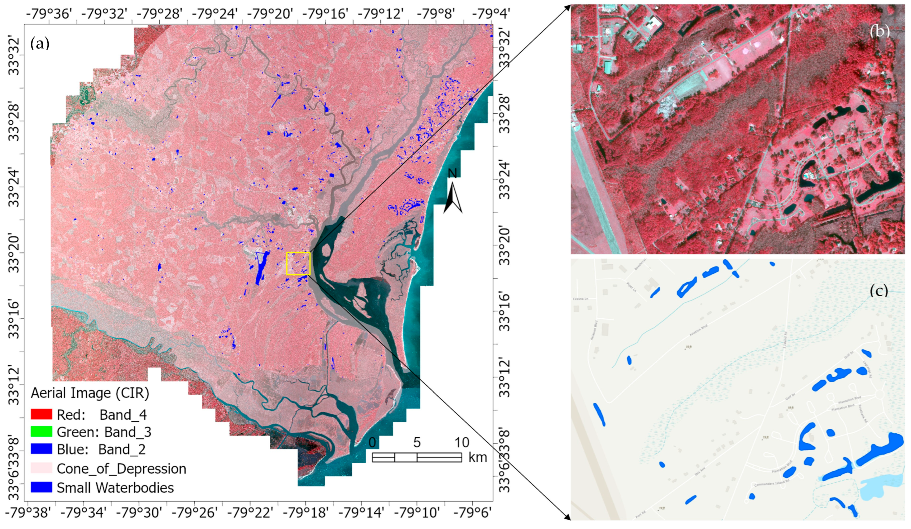
2.1. Study Area and Datasets

Georgetown County at South Carolina is located in the coastal plain, characterized by coastal terraces with low relief ranging from 0 to 47 m above mean sea level [18]. The Pee Dee River gently flows into Winyah Bay, presenting numerous near-pristine river bottomlands, swamps, and estuaries across the floodplain. Geological features include extensive deposits of off-shore limestone from sea rise and fall, as well as sandy sediments eroded from upper lands of the state, comprising a rich set of aquifers and confining layers underground. There are 46 state-permitted wells in this county for which about 80% of the groundwater demand is for water supply [19]. In the potentiometric map of the wells monitored by the SC Department of Natural Resources (SCDNR), substantially lower groundwater levels in confined coastal aquifers were observed in southern Georgetown County, the so-called ‘Cone of Depression’, as revealed by the concentrated iso-water level contours in Figure 1a. Some studies indicated that this spatially extensive pattern was likely due to high-capacity public water supply withdrawals [19,20]. In this study, the subset area in Figure 1a was selected to investigate surface water availability at this Cone of Depression.

In January–March 2020, the statewide aerial imagery was collected with a digital frame camera at 15 cm resolution with four spectral bands (blue, green, red, and near-infrared). The imagery was orthorectified with ground mean errors of georeferencing < 1.5 ft [9]. As shown in the false-color composite (Figure 1b), the study area does not have large lakes or reservoirs but contains numerous small waterbodies.

This study is part of a statewide research project in which 15 cm aerial imagery in Charleston County, with a geographic area of 627 km², was used to train a deep learning model. The training data of small waterbodies were obtained from a recently released 1 m water layer of the NOAA Coastal Change Analysis Program (C-CAP) High-Resolution Land Cover Product [21]. Although smaller waterbodies are often missing in the NOAA C-CAP product, it provides essential training data for deep learning of the 15 cm aerial imagery. After cleaning, a total of 1452 C-CAP waterbodies served as the training set.

Given the interest in small waterbodies, this study utilized the SWOT Level-2 KaRIn High Rate Pixel Cloud product (L2_HR_PIXC), which is primarily intended for terrestrial hydrology. The data product contains the point cloud of pixels within a reloadable water mask. In the pixel cloud, the geolocated water surface heights and complementary attributes are recorded [17]. The L2_HR_PIXC product is available in 64 km × 64 km tile-sized granules. The granules in the study area were downloaded from the NASA Data Platform—EarthData [12].

As a supportive dataset, a 1/9 arc-second (3 m) USGS DEM layer in the study area was downloaded [22]. Since this study was only interested in small, closed waterbodies, rivers and oceanfront open waterbodies like Winyah Bay and numerous tidal channels were not examined. To simplify the process, these open water surfaces were masked from the 2021 NOAA C-CAP water layer product. The mask layer is displayed in Figure 1b.

2.2. Approaches

2.2.1. Deep Learning of the 15 cm Aerial Imagery for Waterbody Classification

As shown in Figure 1b, small waterbodies have distinct boundaries on the false color composite of the 15 cm aerial image. This study takes advantage of the rapidly evolving deep learning technologies to extract small waterbodies from high-resolution imagery. The Mask R-CNN model [10] (He et al. 2017) was adopted after considering the available object-based segmentation networks because it integrates object detection and semantic segmentation to precisely classify the boundary mask for each waterbody.

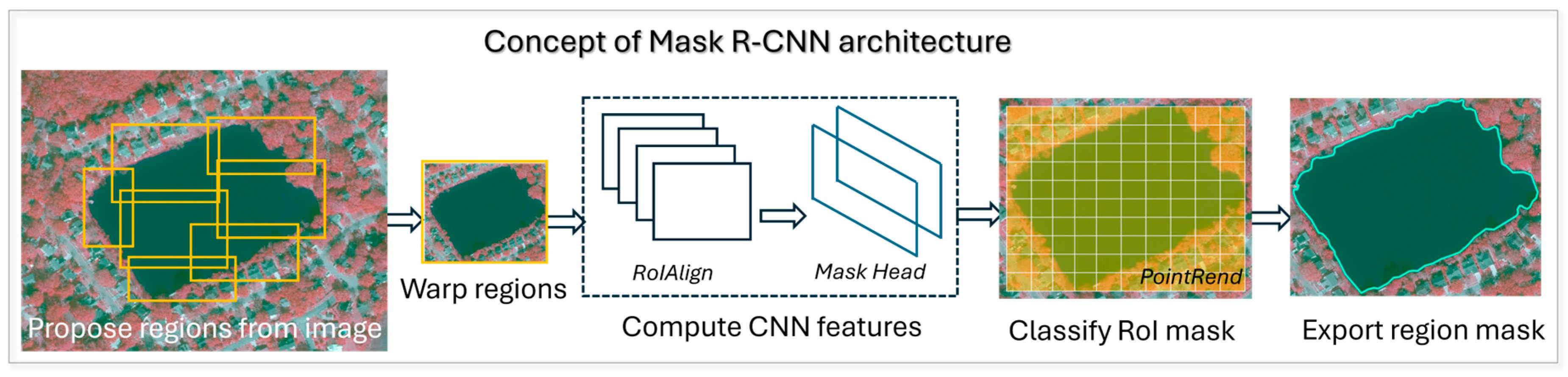
2.2.2. Mask R-CNN Framework

Extended from the Faster R-CNN [10], the Mask R-CNN is processed in three stages (Figure 2). First, the entire image is processed with a backbone network (e.g., ResNet-34 in this study) and a region proposal network to propose a set of regions containing the waterbodies (objects). A proposed region may vary in size depending on the size of the associated waterbody. The second stage contains two convolutional steps. A Region-of-Interest (RoI) pooling method, the RoIAlign pool, splits each proposed region into fixed-size RoIs. At each RoI, the binary prediction is fed into a convolutional neural network to create a feature map (water or no-water). The output then undergoes a two-layer Mask Head convolution to generate each RoI’s water mask in a pixel-to-pixel manner. In the third stage, a point-based rendering neural network module, PointRend Enhancement [23], is added to achieve the precise segmentation of the classified water mask. In this way, the whole image is segmented and the masked RoIs are fully connected to a complete set of waterbody objects.

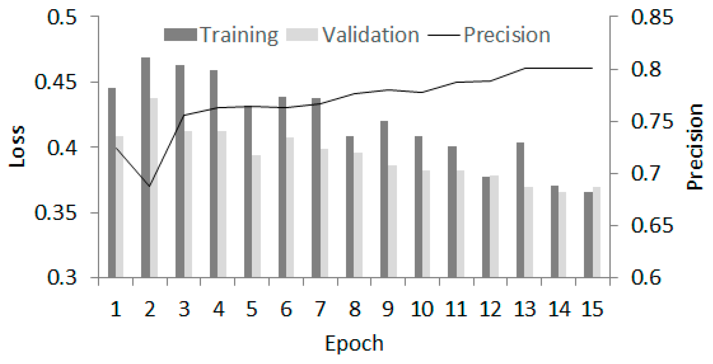
2.2.3. Model Training and Evaluation

As described above, the training set of 1452 waterbodies was collected in earlier efforts on the aerial image at Charleston County. The sizes of these waterbodies range from 205 to 178,515 m², with an average of 4428 m² and median of 1569 m², holding a highly right-skewed histogram. This is reasonable as waterbodies on the U.S. southeast coast are predominantly small. In the labeling process, a tile size of 512 × 512 pixels (around 6000 m²) was chosen to match the average waterbody size in the study area. In the training process, the chip size was selected to be the same as tile size. A total of 90% of the training set was used for model training while 10% was used for validation.

The Mask R-CNN model performance was evaluated using the loss function and precision–recall metrics. For each epoch, the loss function calculates the binary cross-entropy loss. A smaller $Loss$ value represents a better deep learning performance. As an object detection algorithm, the Mask R-CNN model in this study only deals with one object class—waterbody. It exports the conditional probability that an object belongs to waterbody at a user-defined confidence (0.9 in this study). A $True Positive \left(TP\right)$ indicates the waterbody is correctly predicted; a $False Positive \left(FP\right)$ means a non-waterbody is incorrectly predicted as waterbody; and a $False Negative \left(FN\right)$ indicates a waterbody is not predicted. Two metrics were thus calculated:

$$Precision={\displaystyle \frac{TP}{TP+FP}}$$

(1)

$$Recall={\displaystyle \frac{TP}{TP+FN}}$$

$Precision$ measures the proportion of correct predictions among the total predictions, i.e., a measure of commission. $Recall$ is the proportion of correct predictions among the total ground truth, i.e., a measure of omission. Inevitably, the two scores vary with the user-defined confidence thresholds. A smaller threshold reduces $False Negatives$, and hence leads to a higher $Recall$, while a larger threshold reduces $False Positives$ and leads to a higher $Precision$. Therefore, it is tedious and sometimes misleading to solely examine the two scores.

The $Average Precision \left(AP\right)$ is designed to break down the tradeoff between the two metrics. When running the model with a set of threshold values, a $Precision–Recall$ curve (PR curve) can be built by drawing the scatterplot with $Recall$ as the x-axis and $Precision$ as the y-axis. The $AP$ is calculated as the area under the PR curve:

$$AP={\int }_r^{1}Precision\left(r\right)dr$$

(2)

where $r$ is the $Recall$ score along the x-axis of the PR curve, and $Precision\left(r\right)$ is the paired $Precision$ score of the corresponding model prediction.

The $AP$ score ranges from 0 to 1. A high $AP$ score represents both $Precision$ and $Recall$ are high, indicating a good model. A low score means that either metric is low. With this single score, the Mask R-CNN can be evaluated regarding its performance in the extraction of small waterbodies.

2.2.4. SWOT Data Process to Extract the Water Surface Elevation

The SWOT KaRIn instrument measures water surface elevation (WSE). The SWOT PIXC data utilized in this study are a point cloud product in a NetCDF-4 format.

2.2.5. Extracting WSE from SWOT PIXC

The SWOT PIXC product is a point cloud containing 61 attributes of signal observations, Earth surface characteristics, and quality flags [17]. Among the height-related attributes, Height is the measured water surface height above the WGS84 reference ellipsoid. The Geoid records the geoid height, determined from spherical-harmonic Figure models (e.g., EGM2008) of the Earth’s gravity field [24]. In coastal regions, several tidal attributes are recorded in the SWOT PIXC product. In this study area, Solid_earth_tide ($SET$) compensates the subtle deformation of the Earth’s solid surface caused by the gravitational pull of the moon and sun; Load_tide_height ($LT$) deals with the vertical displacement due to tidal loading effect on sea surface height; and Pole_tide_height ($PT$) refers to the vertical displacement from the geocentric pole tide.

We usually refer to a waterbody’s surface height as the height above mean sea level. The abovementioned tidal effects are subtle for terrestrial waterbodies but cannot be neglected in coastal areas. After removing these tidal effects, the WSE above mean sea level is extracted [15,17]:

$${WSE}_i=H_i-{{Geoid}_i-SET}_i-{LT}_i-{PT}_i$$

(3)

where i refers to the pixel point in the SWOT PIXC product.

2.2.6. WSE Noise Reduction

The pixel points in small waterbodies need to be finetuned to reduce noise in WSE measurements. The L2 HR PIXC product contains flag attributes to quantify the KaRIn uncertainties [12]. Two types of uncertainties are evaluated in this study. First, the attribute Classification has seven class types within the pre-defined water mask: land, land near water, water near land, open water, dark water, low-coherence water near land, and open low-coherence water. This study keeps the pixel points in the first four classes. The dark water class refers to pixels lacking detectable radar signals. The low-coherence water classes indicate radar signals with a low level of coherence and, therefore, low measurement quality. Pixel points in these classes are removed. Secondly, the uncertainty in the positioning of the pixel points is evaluated. All pixel points in the PIXC product contain a geolocation_qual flag about the geolocation (height, latitude, and longitude) quality. A higher flag value indicates either suspect, degraded, or bad data quality. In the JPL D-56411 report [17], pixel points with geolocation_qual values higher than 33,554,432 (Bit# 25) are flagged as having bad data quality, and those higher than 65,536 (Bit# 16) are flagged as degraded. These points are also flagged as noise.

After the initial noise removal, the pixel points that fell within the image-classified waterbody polygons were extracted. The WSE value at each point was calculated with Equation (3). Depending on the waterbody size, the number of points at each waterbody could range from 0 to more than one thousand points in the study area.

We assume the water surface of a small waterbody is relatively flat. The WSE values of the pixel points, however, still contain noises that are not systematically flagged, such as the impacts of tall objects (e.g., trees and buildings) on the bank of waterbodies. Here, a simple statistical method is proposed to further smooth the pixel points. For a waterbody polygon with three or more pixel points, set the mean ± standard deviation of WSE values as the confidence envelope and remove all points with WSE beyond the envelope. Repeat the process until the largest deviation between the lowest and highest WSEs in a waterbody is less than 1 m. Using the remaining points, the WSE values are averaged and used as the waterbody’s WSE. Extremely small waterbodies, for example, those only containing 1–2 SWOT pixel points, are excluded.

2.2.7. Exploring WSE Spatial Patterns Indicating Freshwater Availability

The SWOT-extracted WSE on each small waterbody defines the height of surface water above mean sea level. Via spatial interpolation, the WSE layer provides a geostatistical approximation of the upper limit of surface water (without considering flowing water in rivers and open water) across the study area. As shown in Figure 1a, previous SCDNR hydrogeological studies that took place at the monitoring wells reported a Cone of Depression of groundwater in confined aquifers. Although they are from different systems (surface water vs. groundwater), on the oceanfront, like in this study area, the surface of waterbodies could be close to the water table, i.e., the upper surface of unconfined surficial aquifers. Therefore, the WSE layer in this study may provide indirect, supportive information about the Cone of Depression phenomenon.

An Empirical Bayesian Kriging (EBK) approach [25] was adopted to perform a geostatistical interpolation of the WSE of small waterbodies. An exponential semivariogram model was applied in kriging. Additionally, empirical regression with terrain variations was involved in the kriging prediction to examine environmental dependency. Understandably, the elevation of the waterbodies was higher in the upland than the lowlands on the coast. Elevation thus served as the explanatory variable in the EBK regression. Finally, the resulting WSE layer was visually compared with the SCDNR-published Cone of Depression contour map to indicate the feasibility of using SWOT data in water availability assessments.

3. Results and Discussion

3.1. Waterbody Classification Via Deep Learning

Small waterbodies were identified from the aerial image using the Mask R-CNN model. As shown in Figure 3, within 15 epochs, the loss scores of both the training and validation sets gradually decreased to 0.37. The Precision scores at each epoch increased and became stable at 0.8. The $Average Precision \left(AP\right)$ score reached 0.807. Given a confidence threshold of 0.9, this model was capable of detecting small waterbodies in the study area but contained more false positive (commission) errors. By visually exploring the extracted polygon layer, the false positives were primarily found to derive from swamps in riverine and coastal ecosystems. At the 15 Cm resolution, these swamps were easily identified and removed via visual interpretation.

Located on the oceanfront, the study area embraces numerous waterbodies in small sizes. A total of 1112 small waterbodies were extracted from the aerial image (Figure 4a). Their sizes ranged from 167 to 178,367 m² (0.02–17.8 ha) except for the largest lake, Wraggs Bay located at (79°21′ W and 33°19′ N), which has an area of 1,517,160 m² (152 ha). A small subset in a coastal neighborhood was randomly selected to showcase the deep leaning model performance. On the subset image in color infrared composite (Figure 4b), small waterbodies in black are clearly distinctive. As shown in Figure 4c, their polygons are accurately extracted even for the smallest waterbodies in 0.03–0.05 ha in the subset.

3.2. WSE Extraction from SWOT Pixel Cloud

The WSE measurements of the SWOT PIXC product are extremely noisy. Among all pixel points within the image-extracted waterbodies, 56% of them were removed (5524 out of 9856 pixel points) to satisfy the condition of a <1 m difference between the lowest and highest points. To provide a visual demonstration, Figure 5 demonstrates the pixel points within Wraggs Bay. Given the assumption that the water surface of a small waterbody is flat, the water levels should be relatively stable. According to the raw pixel points in Figure 5a, the original WSE values vary dramatically in Wraggs Bay, ranging from 0.11 m at the lowest to 20.58 m at the highest. This wide spam is not reasonable and should be cleaned before application. After noise removal in Figure 5b, the WSE values of the lake fell within a narrower range of 5.23–6.20 m, indicating reasonable water height measurement from the SWOT satellite. A few small waterbodies were observed close to Wraggs Bay. Their WSEs also became more stable after noise removal. Figure 5 also demonstrates the temporal change in small waterbodies. Some waterbodies on the world topography map have dried up or been converted to built-up land on the 2020 aerial image.

The waterbody size determines the number of valid SWOT pixel points it may contain. After noise removal, only 483 out of 1112 image-extracted waterbodies contained valid SWOT pixel points (Figure 6a). The black-bar histogram in the figure reveals these waterbodies have predominantly small sizes (<1 ha). There are only seven waterbodies with an acreage greater than 10 ha. The smallest waterbody is 0.02 ha, containing two valid SWOT pixel points. Contrarily, the exceptionally large waterbody, Wragges Bay, contains 1096 points. The white-bar histogram in the figure presents the average number of SWOT pixel points per waterbody. Apparently, the number of valid SWOT pixel points in a waterbody increases with the size of the waterbody. It ranges from 2 points per waterbody in small-size ones to 193.6 points per waterbody for those greater than 10 ha.

The average WSE of a waterbody was calculated using all valid SWOT pixel points on its water surface. At each pixel point, the USGS DEM was extracted in a 3 × 3 window. The average DEM at all pixel points in a waterbody approximated its bottom elevation. The average WSE and DEM values of the 483 waterbodies presented a positive, linear relationship with Pearson’s r = 0.62. At a freedom of 481, the relationship was statistically significant (p = 0.00). In the WSE-DEM scatterplot heatmap (Figure 6b), the linear relationship is visually clear although it contains large deviations. Using a kernel density approach, the points with higher densities in the scatterplot were colored in a yellowish tone and those in lower densities (sparse points in the scatterplot) were colored in a dark bluish tone. The high deviations were mostly from sparse points, which may be jointly attributed to the uncertainties in the remaining WSE noises and the bottom elevation. For waterbodies in which LiDAR returns are not available, the USGS DEM product is hydro-flattened to calculate their bottom elevations at a 1/9 arcsecond grid size.

3.3. WSE Spatial Patterns at Cone of Depression

The water levels of small waterbodies reveal reasonable geographic patterns across the study area (Figure 7a). In alignment with terrain variations, waterbodies close to the shoreline and tidal rivers have low WSE values of 0–3 m above mean sea level. For inland waterbodies in the west, the WSE values are mostly higher than 12 m. Along the Great Pee Dee River in the northeast end, there are four waterbodies with abnormally high WSE values above 20 m (red dots in Figure 7a) at a relatively low elevation of 2 m (red circle in Figure 6b). These WSE values are unreasonably high and should be counted as errors. However, the pixel points in the four waterbodies were not flagged in the PIXC product or recognized as noises in the proposed noise removal approach in this study.

To better visualize the spatial pattern of surface water levels, a WSE raster layer was extracted from the EBK interpolation (Figure 7b). At 50% transparency, the WSE layer was overlaid on the SCDNR groundwater contour map. The SWOT-extracted WSE represents the upper level of the surface water while the SCDNR contour map shows the groundwater in underlying aquifers. Therefore, their absolute values do not match and are not comparable. Rather, the two map layers reveal similar spatial patterns. For example, the lowest groundwater contour was located at the center of the study area, which also has the lowest WSE range along the tidal channel flowing into Winyah Bay in the southeast. The center of depression on the contour map is reflected by a number of small waterbodies with the lowest SWOT pixel points on the WSE map. The contour lines from the center of depression to the west show a graduate increase in groundwater level, which is also reflected on the WSE map. Interestingly, the abnormally high WSE values in the northeast are supported by the contour map, which reveals a high groundwater level. The discrepancies were observed close to the shoreline. The contour lines still indicate a gradual increase in groundwater level from the center of the depression to the shoreline. However, the WSE map indicates apparently low surface water levels close to Winyah Bay and ocean. The locally high WSE values are supported at the monitoring wells (e.g., GEO-282), in between open waters.

Previous studies indicated that the Cone of Depression phenomenon may be related to the increased groundwater use on the southeast U.S. coast [18]. In conjunction with the growing population of Georgetown County, the higher demand for freshwater requires higher-capacity pumping from the underlying aquifers, which lowers the pressure surface and causes land surfaces to sink and saltwater to intrude on freshwater zones. While the spatial patterns of the WSE layer in this study roughly agree with the Cone of Depression, satellite observations depict the surface water system while the groundwater contours show the groundwater system. However, the two systems can be interrelated in certain ways. One good example is the large number of small wildlife ponds commonly observed on the southeastern U.S. coast [26]. In dry seasons, when precipitation is limited, groundwater is pumped from wells to fill these ponds for wildlife water use. Advanced hydrologic modeling is needed to explore the complex relationships between the two systems and to gain a better understanding of this phenomenon.

3.4. SWOT Point Cloud—Limitations and Research Advances

Previous validation efforts have proven the applicability of SWOT raster and vector data products to measure surface water elevation in large lakes and rivers. For small waterbodies, water-level height measurements are noisy in nature. The Level-2 SWOT PIXC product smoothed the rare interferogram with a medium-level multilooking (~40 looks) procedure in order to optimize the noise-versus-resolution tradeoff of pixel points. This additional spatial averaging achieves approximately 20 m in the along-track and 10–70 m in the cross-track directions [17,27]. Although it has a finer spacing than the Level-2 100 m or 250 m raster products, the interferometric radar signals in a slant view are inevitably affected by water–land interactions on small waterbodies. Their geolocated 3D attributes (latitudes, longitudes, and heights) are thus noisier than those on large waterbodies in terrestrial lands. However, a visual examination of the noise-cleaned pixel points in Wraggs Bay (see Figure 5) did not reveal a clear WSE transition of pixel points from the lake center to the bank, indicating that significant system noise remained after noise removal. To compensate, a threshold of 1 m was used in the proposed noise removal approach, i.e., the WSE difference between the lowest and highest pixel points in a waterbody could not be greater than one meter. Future investigations with intensive real-time field experiments are needed to clarify the sources of this noise (systematic vs. environmental) and to perform a solid WSE validation using SWOT pixel points.

The availability of high-resolution imagery, advancements in deep learning, and the recent SWOT satellite observations have enabled unprecedented measurements of terrestrial water levels. Geographically, small waterbodies are often ignored in water studies because they are heavily contaminated with mixed pixels on satellite imagery. Sub-meter aerial imagery was operationally adopted in federal/state agencies and private sectors. The 15 cm aerial imagery used in this study is a statewide effort from the South Carolina legislature to support a wide range of public services. For water-level measurements, SWOT data products are available in an 11-day revisit cycle. Past studies [28] have indicated the feasibility of extracting volumes of in-land waterbodies utilizing satellite altimetry and high-resolution surface areas, as well as bathymetric data, in hydrological modeling. Taking advantage of SWOT surface water-level layers and groundwater records at established stations, the approaches presented in this study may lead to a precise way of identifying hydrological basins and defining the surface boundary conditions of small waterbodies for hydro-models to simulate water storage and the temporal dynamics of small waterbodies.

Integrating these remotely sensed datasets with the in situ monitoring records and groundwater modeling framework, the 3D documentation of small waterbodies provides useful information on freshwater availability and spatiotemporal variations. Due to the accelerated pressure from climate change and urbanization on the coast, such information is critical to assist in the sustainable water-use planning of small waterbodies.

4. Conclusions

This study demonstrates the usefulness of high-resolution imagery and the new SWOT PIXC product in the 3D measurements of small waterbodies. In a case study of coastal areas in South Carolina, USA, small waterbodies were extracted via deep learning of a 15 cm aerial image, and their water surface elevations (WSE) are calculated from the SWOT PIXC pixel cloud. Major findings include the following:

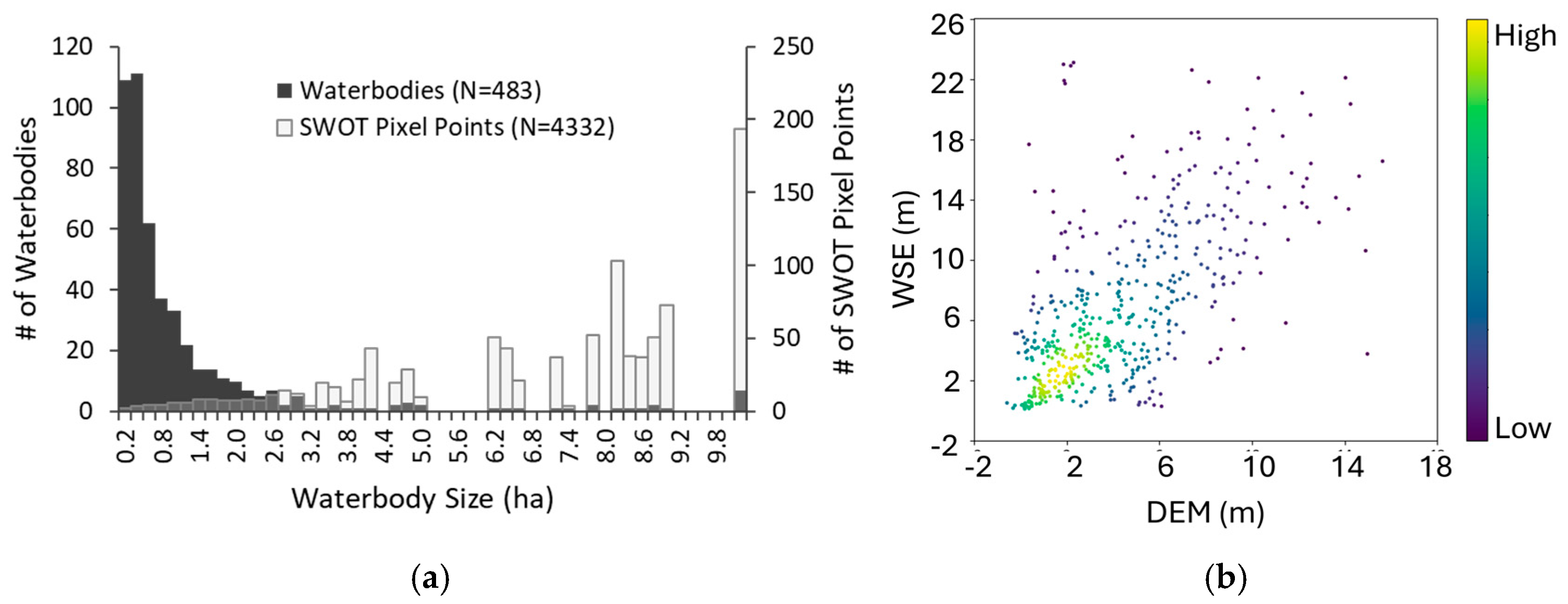
• A total of 1112 small waterbodies were detected using the Mask R-CNN model, with an average precision of 0.81. The smallest waterbody had a size of 0.02 ha.
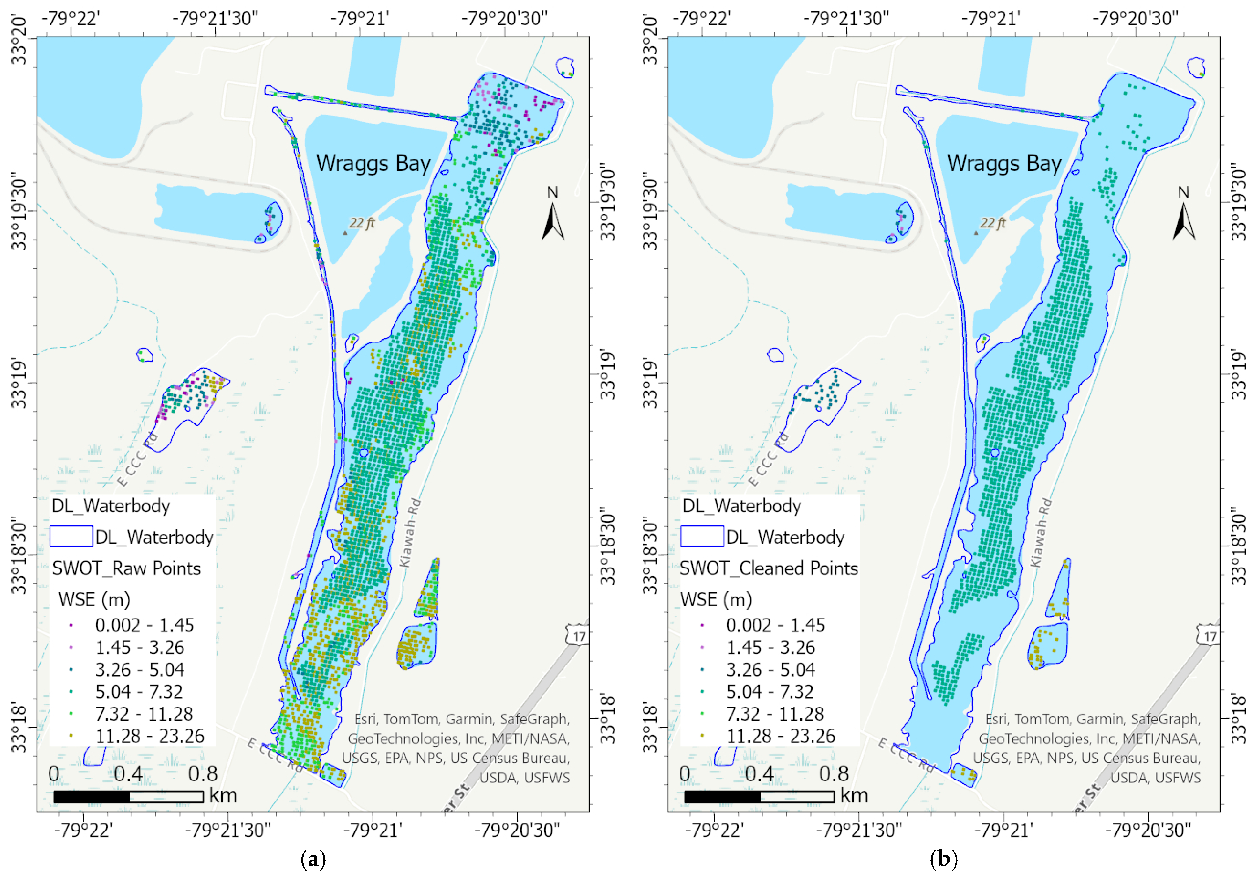
• The SWOT PIXC pixel points in small waterbodies are noisy in nature. After noise removal, only 483 of the 1112 waterbodies contained valid pixel points, varying from 2 points per waterbody in the smallest sizes and 193.6 points per waterbody in sizes > 10 ha.
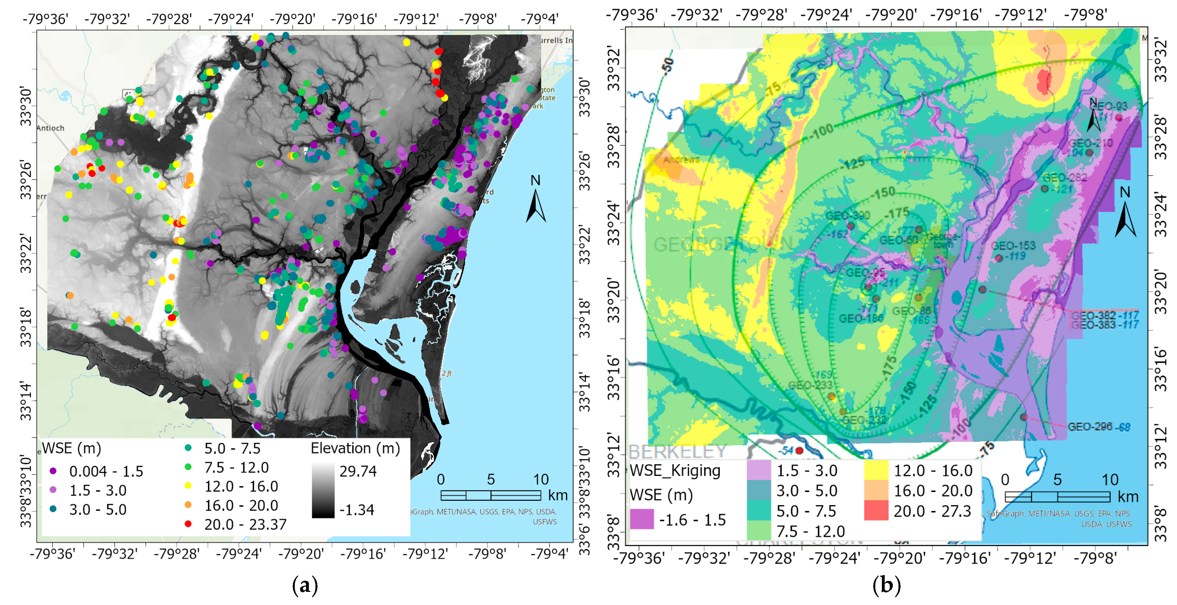
• The surface water levels of small waterbodies are significantly related to elevations across the study area (Pearson’s r = 0.62). The spatially interpolated WSE patterns generally agree with the groundwater contours in the central Cone of Depression but not along the oceanfront, increasing hydro-modeling interest in better understanding this phenomenon.

This study serves as a first attempt to evaluate the feasibility of using the SWOT PIXC product to document the water levels of terrestrial small waterbodies. With further validation from real-time field experiments, the SWOT water-level measurements of small waterbodies will provide valuable information for water storage assessments, supporting the state’s resilient water use.

References

1. Hill, M.J.; Greaves, H.M.; Sayer, C.D.; Hassall, C.; Milin, M.; Milner, V.S.; Marazzi, L.; Hall, R.; Harper, L.R.; Thornhill, I.; et al. Pond ecology and conservation: Research priorities and knowledge gaps. Ecosphere 2021, 12, e03853. [Google Scholar] [CrossRef]
2. Biggs, J.; von Fumetti, S.; Kelly-Quinn, M. The Importance of Small Waterbodies for Biodiversity and Ecosystem Services: Implications for Policy Makers. Hydrobiologia 2017, 709, 3–19. [Google Scholar] [CrossRef]
3. Moore, R.B.; McKay, L.D.; Rea, A.H.; Bondelid, T.R.; Price, C.V.; Dewald, T.G.; Johnston, C.M. User’s Guide for the National Hydrography Dataset Plus (NHDPlus) High Resolution; U.S. Geological Survey Open-File Report 2019–1096; USGS: Reston, VA, USA, 2019; 66p. [CrossRef]
4. South Carolina Department of Natural Resources (SCDNR). South Carolina LiDAR Data. 2024. Available online: https://www.dnr.sc.gov/GIS/lidar.html (accessed on 29 December 2024).
5. SC Water Resources Center (SCWRC). Inventory of Lakes in South Carolina: Ten Acres or More in Surface Area; SCWRC Report 171; U.S. Army Corps of Engineers: Columbia, SC, USA, 1991.
6. Qayyum, N.; Ghuffar, S.; Ahmad, H.; Yousaf, A.; Shahid, I. Glacial lakes mapping using multi satellite PlanetScope imagery and deep learning. ISPRS Int. J. Geo-Inf. 2020, 9, 560. [Google Scholar] [CrossRef]
7. Mullen, A.L.; Watts, J.D.; Rogers, B.M.; Carroll, M.L.; Elder, C.D.; Noomah, J.; Williams, Z.; Caraballo-Vega, J.A.; Bredder, A.; Rickenbaugh, E. Using high-resolution satellite imagery and deep learning to track dynamic seasonality in small water bodies. Geophys. Res. Lett. 2023, 50, e2022GL102327. [Google Scholar] [CrossRef]
8. Sun, D.; Gao, G.; Huang, L.; Liu, Y. Extraction of Water Bodies from High-resolution Remote Sensing Imagery Based on a Deep Semantic Segmentation Network. Sci. Rep. 2024, 14, 14604. [Google Scholar] [CrossRef] [PubMed]
9. SC Revenue and Fiscal Affairs Office (SCRFA). SC Aerial Imagery Program. 2024. Available online: https://rfa.sc.gov/programs-services/geodetic/statewide-aerial-imagery (accessed on 29 December 2024).
10. Ren, S.; He, K.; Girshick, R.; Sun, J. Faster R-CNN: Towards Real-Time Object Detection with Region Proposal Networks. IEEE Trans. Pattern Anal. Mach. Intell. 2017, 39, 1137–1149. [Google Scholar] [CrossRef] [PubMed]
11. Fu, L.L.; Pavelsky, T.; Cretaux, J.F.; Morrow, R.; Farrar, J.T.; Vaze, P.; Sengenes, P.; Vinogradova-Shiffer, N.; Sylvestre-Baron, A.; Picot, N.; et al. The surface water and ocean topography Mission: A breakthrough in radar remote sensing of the ocean and land surface water. Geophys. Res. Lett. 2024, 51, e2023GL107652. [Google Scholar] [CrossRef]
12. Surface Water Ocean Topography (SWOT). SWOT Science Data Products User Handbook (JPL D-109532); NASA Jet Propulsion Laboratory (JPL): Pasadena, CA, USA, 2024. Available online: https://podaac.jpl.nasa.gov (accessed on 29 December 2024).
13. Maubant, L.; Dodd, L.; Tregoning, P. Assessing the accuracy of SWOT measurements of water bodies in Australia. Geophys. Res. Lett. 2025, 52, e2024GL114084. [Google Scholar] [CrossRef]
14. Yao, J.; Xu, N.; Wang, M.; Liu, T.; Lu, H.; Cao, Y.; Tang, X.; Mo, F.; Chang, H.; Gong, H.; et al. SWOT satellite for global hydrological applications: Accuracy assessment and insights into surface water dynamics. Int. J. Digit. Earth 2025, 18, 2472924. [Google Scholar] [CrossRef]
15. Yu, L.; Zhang, H.; Gong, W.; Ma, X. Validation of Mainland Water Level Elevation Products from SWOT Satellite. IEEE J. Sel. Top. Appl. Earth Obs. Remote Sens. 2024, 17, 13494–13505. [Google Scholar] [CrossRef]
16. Zhao, Y.; Fu, J.; Pang, Z.; Jiang, W.; Zhang, P.; Qi, Z. Validation of Inland Water Surface Elevation from SWOT Satellite Products: A Case Study in the Middle and Lower Reaches of the Yangtze River. Remote Sens. 2025, 17, 1330. [Google Scholar] [CrossRef]
17. Surface Water Ocean Topography (SWOT). SWOT Product Description—Level 2 KaRIn High Rate Water Mask Pixel Cloud Product, REVISION C (JPL D-56411); NASA Jet Propulsion Laboratory (JPL): Pasadena, CA, USA, 2024. Available online: https://podaac.jpl.nasa.gov/dataset/SWOT_L2_HR_PIXC_2.0 (accessed on 29 December 2024).
18. Campbell, B.G.; Fine, J.M.; Petkewich, M.D.; Coes, A.L.; Terziotti, S. Chapter A: Groundwater Availability in the Atlantic Coastal Plain of North and South Carolina. In Groundwater Availability in the Atlantic Coastal Plain of North and South Carolina; Campbell, B.G., Coes, A.L., Eds.; Professional Paper 1773; USGS: Reston, VA, USA, 2010; p. 2. [Google Scholar]
19. Kemmer, C.; Wyant, P.; Hughes, J.; Koon, J.M.; Monroe, L.A. Waccamaw Capacity Use Area Groundwater Evaluation Report, Permitting Year 2024; Technical report Number 006-2023; South Carolina Department of Health and Environmental Control (DHEC): Columbia, SC, USA, 2023.
20. Gellici, J.A.; Lautier, J.C. Chapter B: Hydrogeologic Framework of the Atlantic Coastal Plain, North and South Carolina. In Groundwater Availability in the Atlantic Coastal Plain of North and South Carolina; Campbell, B.G., Coes, A.L., Eds.; Professional Paper 1773; USGS: Reston, VA, USA, 2010; p. 241. [Google Scholar]
21. National Oceanic and Atmospheric Administration (NOAA). Coastal Change Analysis Program (C-CAP) High-Resolution Land Cover; NOAA Office for Coastal Management: Charleston, SC, USA, 2021. Available online: https://coast.noaa.gov/digitalcoast/data/ccaphighres.html (accessed on 29 December 2024).
22. U.S. Geological Survey (USGS). USGS 3D Elevation Program Digital Elevation Model. 2019. Available online: https://apps.nationalmap.gov/downloader/ (accessed on 29 December 2024).
23. Kirillov, A.; Wu, Y.; He, K.; Girshick, R. PointRend: Image Segmentation as Rendering. arXiv 2019, arXiv:1912.08193. [Google Scholar]
24. Pavlis, N.K.; Holmes, S.A.; Kenyon, S.C.; Factor, J.K. The development and evaluation of the Earth Gravity Model 2008 (EGM2008). J. Geophys. Res. Solid Earth 2022, 117, 1978–2012. [Google Scholar]
25. Krivoruchko, K.; Gribov, A. Evaluation of empirical Bayesian kriging. Spat. Stat. 2019, 32, 100368. [Google Scholar] [CrossRef]
26. White, S.A.; Beecher, L.; Davis, R.H.; Nix, H.B.; Sahoo, D.; Scaroni, A.E.; Wallover, C.G. Ponds in South Carolina. Land-Grant Press by Clemson Extension. 2021. Available online: https://lgpress.clemson.edu/publication/ponds-in-south-carolina/ (accessed on 31 March 2025).
27. Salameh, E.; Desroches, D.; Deloffre, J.; Fjørtoft, R.; Mendoza, E.T.; Turki, I.; Froideval, L.; Levaillant, R.; Déchampt, S.; Picot, N.; et al. Evaluating SWOT’s interferometric capabilities for mapping intertidal topography. Remote Sens. Environ. 2024, 314, 114401. [Google Scholar] [CrossRef]
28. Schwatke, C.; Dettmering, D.; Seitz, F. Volume Variations of Small Inland Waterbodies from a Combination of Satellite Altimetry and Optical Imagery. Remote Sens. 2020, 12, 1606. [Google Scholar] [CrossRef]
Figure 1. The study area: (a) the Cone of Depression in Southern Georgetown County, SC (Gellici, J.A. and Lautier, J.C. 2010, in Campbell, B.G. & Coes, A.L. (Eds.), USGS Professional Paper 1773 [20]); (b) the 2020 aerial image, shown in color infrared composite.
Environments 12 00168 g001
Figure 2. The Mask R-CNN architecture for small waterbody extraction.
Environments 12 00168 g002
Figure 3. The training performance of the Mask R-CNN model.
Environments 12 00168 g003
Figure 4. The Deep Learning-classified waterbody polygons overlaid on the aerial image (a). A subset image (b) is displayed for better visualization of the extracted small waterbodies (c).
Environments 12 00168 g004
Figure 5. The WSE measurements of SWOT pixel points in the area of Wraggs Bay before (a) and after (b) noise removal.
Environments 12 00168 g005
Figure 6. The histograms of waterbodies and valid SWOT pixel points for waterbody size (a) and the colored WSE-DEM scatterplot heatmap (b).
Environments 12 00168 g006
Figure 7. The SWOT-extracted WSE values of small waterbodies overlaid on DEM (a). The EBK-interpolated WSE map (50% transparency) overlaid on the SCDNR groundwater contours (b).
Environments 12 00168 g007
Disclaimer/Publisher’s Note: The statements, opinions and data contained in all publications are solely those of the individual author(s) and contributor(s) and not of MDPI and/or the editor(s). MDPI and/or the editor(s) disclaim responsibility for any injury to people or property resulting from any ideas, methods, instructions or products referred to in the content.