Assessing the Impacts of Climate Change on Hydrological Processes in a German Low Mountain Range Basin: Modelling Future Water Availability, Low Flows and Water Temperatures Using SWAT+

Abstract

This study assesses the projected impacts of climate change on hydrological processes in the Gersprenz catchment, a representative low mountain range basin in central Germany, under the RCP8.5 scenario. Using the SWAT+ model and a bias-corrected climate projection ensemble, it simulates the temporal and spatial dynamics of water availability, discharge and water temperature through 2100. The results indicate a substantial reduction in seasonal discharge, with summer minima decreasing by 85% and autumn minima decreasing by 38% compared to the baseline. Rising air temperatures drive substantial warming, with maximum summer water temperatures projected to exceed 28 °C, increasing thermal stress on aquatic ecosystems. Spatial analysis reveals strong variability: Southern subcatchments, located in the upstream part of the catchment, face severe water deficits, while groundwater-fed springs provide localized thermal refuges but with limited buffering capacity. Northern regions generally show higher resilience, with exceptions. The findings highlight the fine-scale sensitivity of hydrological processes to climate change, shaped by catchment characteristics and amplified by natural seasonal variations. This study presents a framework for identifying spatio-temporal hotspots of water scarcity at the subcatchment scale, providing a basis for spatially targeted adaptation strategies to mitigate the impacts of climate change on regional water resources and ecosystems.

1. Introduction

Climate change is increasingly impacting hydrological systems worldwide, altering water availability, streamflow dynamics and ecological health [1,2,3,4,5]. Rising temperatures increase evaporation rates and reduce soil moisture, while shifts in precipitation patterns significantly affect the timing, intensity and volume of stream discharge. Together, these changes destabilize hydrological systems, leading to a growing frequency of extreme hydrological events [5,6].

The impacts of climate change on hydrological processes exhibit significant spatial and temporal variability. Regional and seasonal disparities drive heterogeneous hydrological responses, governed by local climatic conditions and catchment-specific characteristics [7]. Across diverse hydroclimatic regions, catchments exhibit distinct sensitivities to climate change, even at the subcatchment scale.

In Germany, rising temperatures and changing precipitation patterns have intensified water scarcity, extreme low flows and elevated water temperatures [8,9]. The exceptional drought and heat year of 2018 was a standout example of these impacts, with nine of Germany’s fifteen major rivers experiencing extreme low flow conditions for more than 100 days [9]. Such low flow conditions have profound ecological and socioeconomic consequences, including warming water bodies, oxygen depletion, ecosystem disruption and escalating conflicts over resource use [9]. With temperatures in Germany projected to rise by up to 4.2 °C on average in the far future [10], the likelihood of prolonged periods of water scarcity, extreme low flows and elevated water temperatures is expected to increase further [11,12].

The occurrence and severity of water scarcity and low flow in Germany exhibit significant variability, driven by regional and seasonal differences in climate, as well as catchment-specific factors such as topography and land use, which influence sensitivities to climate change [12]. These factors modulate hydrological responses, influencing the timing of water availability and the emergence of localized scarcity hotspots. Assessing the impacts of shifting climate variables on hydrological processes at fine scales is therefore critical for accurately predicting water availability and developing targeted management strategies to mitigate water scarcity and drought risks [11]. In this context, hydrological modelling serves as a powerful tool for quantifying these interactions, particularly when integrating high-resolution climate projections with process-based approaches that account for seasonal and spatial heterogeneity, ensuring a more reliable assessment of future hydrological conditions.

The Gersprenz catchment serves as a representative case for studying the impacts of climate change on low mountain range catchments in central Germany. Spanning over 500 km² in southern Hesse, this research catchment was established in 2016 as a field laboratory by the Chair of Engineering Hydrology and Water Management at the Technical University of Darmstadt. Since then, numerous scientific studies have been conducted to comprehensively investigate catchment processes and development dynamics on various scales. These studies aim to provide an integrated understanding of the catchment’s hydrological and environmental system [13,14,15,16,17,18,19,20,21,22,23,24].

In this context, research by Grosser and Schmalz (2023) revealed that the Gersprenz region is projected to experience above-average warming compared to the rest of Germany, with significant increases in dry periods during summer and autumn [17]. Despite wetter winters, prolonged droughts are expected to intensify water stress. A historical analysis of hydrological dynamics in the Gersprenz basin (1980–2018) by Grosser and Schmalz (2021) documented a marked rise in both the frequency and severity of low flow and drought events, with notable subcatchment scale variations that underscore the critical influence of local catchment characteristics [16]. Furthermore, minimal land use changes during this period suggest that these hydrological shifts are predominantly driven by climate variability rather than anthropogenic alterations.

While past trends in low flow conditions and droughts have been examined and climatic trends projected, a comprehensive assessment of how these changes will impact future hydrological processes in the Gersprenz catchment remains lacking. Existing studies indicate historical increases in low flow events alongside anticipated rises in air temperatures and shifts in precipitation patterns. However, key uncertainties persist regarding whether these trends will continue in the intermediate and long term, how rising air temperatures will influence water temperatures and whether the months experiencing the most extreme meteorological changes will align with those of the lowest seasonal discharges. The interplay between reduced discharge and elevated water temperatures—and the potential feedback mechanisms that could exacerbate water scarcity and ecological stress—has yet to be fully explored. Moreover, a significant gap remains in understanding climate change impacts at the subcatchment scale, limiting the ability to assess how distinct hydrological responses may emerge across varying catchment characteristics. To address these shortcomings, this study focuses on investigating the following questions:

• How will projected climate change alter the seasonal dynamics and long-term trends of discharge and low flow events in the low mountain range catchment through 2100?
• How will rising air temperatures influence water temperatures, affecting thermal stress in aquatic ecosystems?
• What spatial differences in hydrological responses exist at the subcatchment level, and how can they be linked to catchment characteristics to identify vulnerable and resilient subcatchments?

To answer these questions, this study employs the Soil and Water Assessment Tool Plus (SWAT+), a widely used hydrological model applicable across diverse catchments [25]. Calibrated with data from 1988 to 2017 and optimized using performance criteria (KGE, PBIAS and low flow accuracy), the model simulates current conditions to provide robust future hydrological projections. Projections are based on the Representative Concentration Pathway 8.5 (RCP8.5) scenario, offering critical insights into the maximum potential impacts of climate change for effective preparedness planning [26,27].

These findings provide a robust framework for understanding the spatial and temporal variability of hydrological changes in a low mountain range catchment under climate change. By identifying areas most vulnerable to water scarcity, prolonged droughts and thermal stress, this study provides a valuable basis for future research on adaptation strategies. The detailed subcatchment-level analysis of low flows and water temperatures enhances the understanding of climate-driven hydrological responses within the catchment, offering valuable insights for water resource management and climate adaptation planning in similar regions. Furthermore, this study highlights the value of process-based hydrological modelling and spatial analysis in assessing water stress within river basins. By examining discharge and water temperature trends alongside low flow metrics across multiple temporal and spatial scales, it establishes a methodology for identifying spatio-temporal hotspots of water scarcity at the subcatchment scale.

2. Methods and Methodology

To address the challenges posed by climate change in the Gersprenz catchment, this study utilizes the SWAT+ hydrological model, a process-based tool widely recognized for its ability to simulate key hydrological processes under varying climatic conditions. This study focuses on projecting future hydrological dynamics, emphasizing water availability, discharge and the behaviour of low flows and water temperatures.

The methodological framework includes a description of the catchment, model setup, calibration and validation, followed by the application of climate scenarios and analysis of temporal and spatial hydrological trends.

Section 2.1 introduces the physical and climatic characteristics of the study area. Section 2.2 details model configuration and calibration processes. Section 2.3 outlines the analytical approaches used to assess seasonal and spatial variability.

Figure 1 presents the workflow, summarizing the steps from model setup and calibration to scenario modelling under RCP8.5. Detailed descriptions of all inputs, adjustments and analysis methods are provided in the following sub-sections.

2.1. Study Area

The Gersprenz catchment is located in the federal state of Hesse in southern Germany and forms part of the Rhine River basin district (Figure 2). It spans approximately 500 km² up to the state border with Bavaria and includes a network of tributaries. The main river originates in the crystalline Odenwald low mountain range and flows northward for 62 km before discharging into the Main River near Stockstadt.Elevations in the catchment range from approximately 600 to 100 m above sea level. The basin exhibits typical characteristics of a German low mountain range catchment, with a mix of silicate-rich crystalline and tertiary deposits. The southern part is characterized by steeper slopes, shallow soils and silicate-rich bedrock, resulting in lower infiltration and higher surface runoff. In contrast, the northern areas transition into more level terrain with loess and clay-rich sediments, supporting deeper infiltration and greater subsurface water retention [28].

Land use is predominantly agricultural (48%), followed by forest (36%) and urban settlements (13%) [22]. Climatic conditions are temperate, with a mean annual temperature of 10.2 °C and average annual precipitation of 642 mm [16,29]. Due to its physiographic and climatic setting, the region is considered particularly vulnerable to hydrological extremes, including drought and low flow events. It is therefore well suited for studying the regional impacts of climate change on water availability.

2.2. Model Setup

This section provides an overview of the input data, model adjustments, sensitivity analysis, calibration and validation steps for setting up the SWAT+ model for the Gersprenz catchment. The modelling period was determined based on the availability of necessary input data such as observed streamflow and meteorological records. This resulted in a model period spanning from 1988 to 2017. How this period was partitioned for calibration and validation is shown in

Table 1. Modelling period.

Modelling Period	01.01.1988 – 31.12.2017	30 Years
Warm-up	1988–1990	3 years
Calibration	1991–2008	18 years
Validation	2009–2017	9 years

.

2.2.1. Data Sources and Model Inputs

Process-oriented models such as SWAT+ rely on extensive spatial and temporal datasets to accurately represent the factors influencing hydrological processes in a catchment. The key data used in this study is summarized in

Table 2. Overview of data sources and model inputs.

	Application	Resolution	Source
Digital Elevation Model (DEM)	Watershed Delineation	5 m	Hessian Administration for Land Management and Geoinformation [30]
Stream Network		-	Official Topographic–Cartographic Information System [31]
Land Cover	Hydrologic Response Units	5 ha	CLC5_2018 [32]
Soil		1:50,000	Soil surface data Hesse [33]
Observed Discharge	Calibration and Validation	Daily	Discharge data of the Gauge Harreshausen [34]
Observed Climate Data		Daily	German Weather Service [29]

.

A 5-m resolution DEM was utilized for watershed delineation and slope determination [30]. To improve the accuracy of the stream network in the Lower Main Valley, a portion of the stream network was burned into the DEM. The catchment boundary was defined by the gauging station Harreshausen. Daily discharge data for this station was provided by HLNUG (2019) and were employed in both the calibration and validation phases of the model [34]. SWAT+ uses land cover, soil data and slope information to define Hydrologic Response Units (HRUs), which represent areas of homogeneous land surface characteristics and hydrological response within a watershed.

Land cover information was derived from the CLC5_2018 dataset at a resolution of 5 ha [32]. The dataset was clipped to the study area, and features were reclassified according to SWAT+ land use categories. Soil data was obtained from the BFD50 database, which provides standardized soil information at a scale of 1:50,000 [33]. Initially, 218 soil classes were identified within the catchment; these were manually generalized to 22 classes based on land use, horizon sequence and relevant hydrological properties to ensure computational efficiency while retaining meaningful representation.

HRUs in this study were generated by identifying unique combinations of land use, soil type and slope class within each subbasin. To limit fragmentation and improve model performance, only combinations covering more than 10% of the subbasin area for land use, 15% for soil and 20% for slope were retained. This thresholding approach filtered out minor combinations while preserving dominant hydrological characteristics. The final model set-up includes 9 subbasins, 39 channels and 572 HRUs across the Gersprenz catchment.

Daily climate data, including precipitation, temperature, wind speed, relative humidity and global radiation, were obtained from the Climate Data Centre of the German Weather Service [29]. Weather stations were selected based on their proximity to subcatchments and data availability, as outlined in

Table 3. Climate data [29].

Station	ID	Latitude	Longitude	Elevation 1	Climate Parameters
Lautertal/ Odenwald-Reichenbach	2900	49.7090	8.6908	208	Precipitation
Michelstadt	3284	49.6691	9.0085	240	Precipitation, rel. humidity, temperature
Michelstadt-Vielbrunn	3287	49.7176	9.0997	453	Precipitation, temperature, wind speed
Roedermark/ Ober-Roden	4230	49.9832	8.8395	137	Precipitation
Schaafheim-Schlierbach	4411	49.9195	8.9671	155	Precipitation, temperature
Wuerzburg	5705	49.7703	9.9577	268	Global radiation
Dieburg	955	49.8975	8.8486	145	Precipitation

¹ Elevation in meters above sea level (m.a.s.l.).

.

2.2.2. Model Adjustments

In SWAT+, various options are available beyond direct parameter adjustments during calibration to fine-tune the model. One key adjustment involved changing the potential evapotranspiration method from the default Penman–Monteith to the Hargreaves method. The Hargreaves method requires less input data, thereby reducing potential uncertainties associated with potential evapotranspiration estimation under climate change projection. All other settings were kept at their defaults, including the variable storage routing for flexible channel flow representation and the Soil Conservation Service (SCS) curve number (CN) method for estimating surface runoff.

In addition, SWAT+ allows for the integration of management practices to simulate specific land use scenarios. For the model of the Gersprenz catchment, land and forest management practices were incorporated to improve the representation of vegetation growth and land use dynamics. These adjustments were designed to enhance the model’s accuracy in simulating key water balance components, including evapotranspiration, infiltration and runoff, providing a more realistic depiction of the catchment’s hydrological processes.

With agricultural land comprising approximately 50% and forestry covering about 35% of the catchment, management practices in these areas play a critical role in shaping the water cycle. Given the focus on the projection of quantitative stream flow hydrology in this study, a simplified management schedule was tailored for the agricultural area, combining the three most prominent crops in Hesse—rapeseed, winter wheat and winter barley (CANA-WWHT-WBAR) [35]. This schedule, which includes planting dates, fertilization, tillage and harvest timing, was based on data provided by the Curatorium for Technology and Engineering in Agriculture [36].

For pasture, automated decision tables were introduced to model hay cutting, fertilization and grazing during both summer and winter seasons, addressing an overestimation of pasture biomass under default settings. The resulting biomass levels aligned with expected values of approximately 4 t/ha [37].

Initial SWAT+ model runs with default settings in the plant database showed a declining trend in biomass over time (Figure 3). Further analysis identified misrepresentation of forest biomass as the primary cause of this discrepancy. Forests account for a significant proportion of the total biomass in the study area. The model failed to reproduce the biomass levels reported by the Federal Forest Inventory [38,39].

The model includes three forest types: deciduous forest (FRSD), mixed forest (FRST) and evergreen forest (FRSE). To improve the accuracy of the biomass modelling, adjustments were made to the plant database based on an extensive literature review of the dominant tree species within these forest types [40,41,42,43]. These adjustments, detailed in

Table 4. Adaptation in plant database for deciduous forest (FRSD), mixed forest (FRST) and evergreen forest (FRSE) [40,41,42].

	FRSD	FRST	FRSE
bm_max [t/ha] (Maximum Biomass)	275	250	200
Years to Maturity	100	95	80
Maximum Canopy Height [m]	30	50	50
Maximum Root Depth [m]	1.6	2	1.2
Optimal Temperature for growth [°C]	20	17	13
Minimum T [°C]	0	0	0
Bio_e (Biomass Energy Ratio)	20	20	15

, corrected biomass estimates and prevented unrealistic declines.

Additionally, management plans for forest harvesting were integrated into the model [42,44]. Model runs with the adapted settings ensured expected biomass levels. The resulting biomass for each forest type and the corresponding leaf area indices (LAI) are shown in Figure 4.

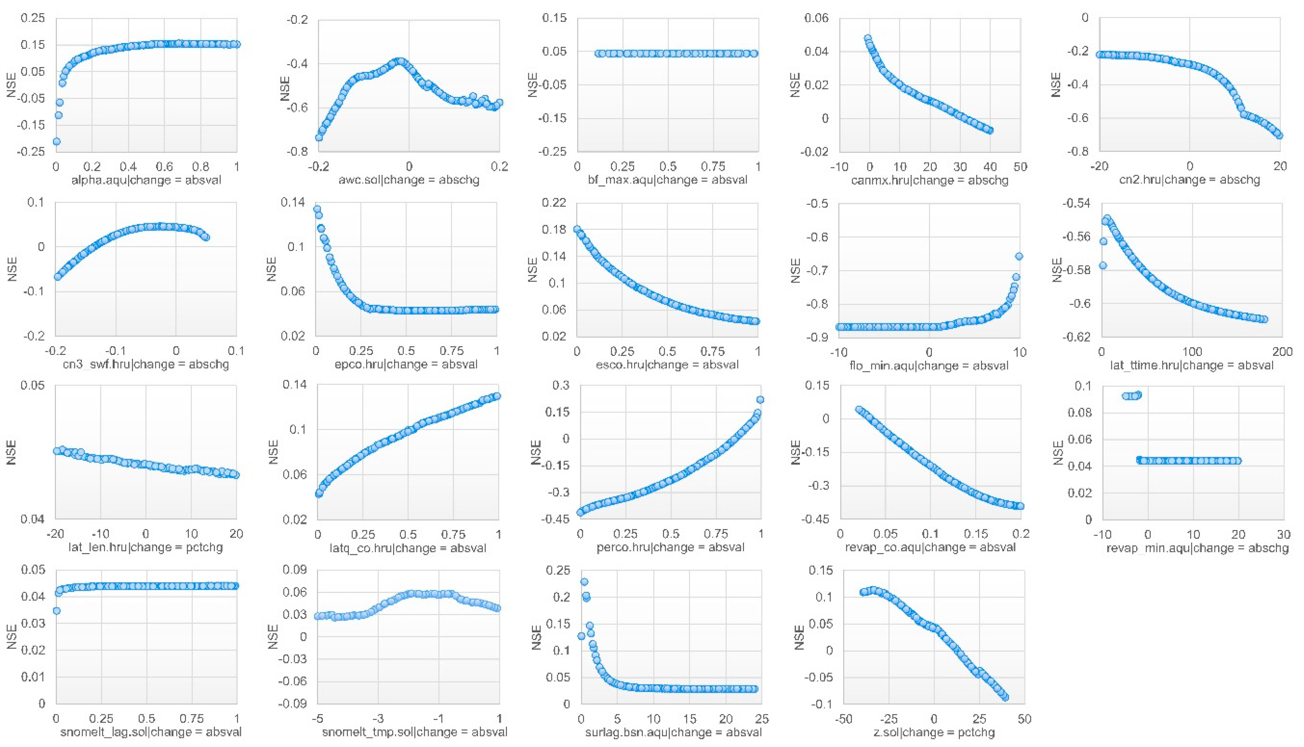
2.2.3. Sensitivity Analysis

After configuring and refining the model to achieve an adequate representation of watershed dynamics, including vegetation growth and water balance components, a sensitivity analysis was conducted to identify the parameters most influential on the modelled discharge output. This step is essential in understanding the model’s behaviour and for prioritizing key parameters for calibration.

In total, 19 parameters were tested for sensitivity in the SWAT+ hydrological model using a Latin Hypercube-One-At-a-Time (LH-OAT) method, following the framework of Morris’ Screening Method [45,46]. In this approach, Latin Hypercube (LH) sampling was used to efficiently explore the parameter space, while the One-At-a-Time (OAT) technique was applied to evaluate the influence of individual parameter changes on model performance. An R script from the SWATplusR framework was used to facilitate the sensitivity analysis [47]. Figure 5 illustrates how model performance (NSE) responds to changes in each parameter across its defined range.

Following the identification of sensitive parameters, a manual sensitivity analysis was performed using the SWAT+ toolbox to precisely evaluate the influence of each parameter on the water balance components [48]. This analysis ensured that parameter selection did not result in unrealistic or disproportionate relationships among the components of the water balance, thereby maintaining the model’s hydrological plausibility.

2.2.4. Calibration and Validation

Calibration was performed using the SWATplusR framework for the period 1991–2008 [47]. A total of 7000 parameter combinations were sampled using Latin Hypercube (LH) sampling within ranges defined by hydrological plausibility and insights gained from the sensitivity analysis. The number of runs was the result of an explorative, iterative process balancing model performance and computational feasibility.

Given this study’s focus on climate change impacts on overall water availability and low flow dynamics, the following goodness-of-fit metrics were prioritized during calibration: Percent Bias (PBIAS), Kling–Gupta Efficiency (KGE) and very low flow.

PBIAS quantifies whether the modelled data tend to overestimate or underestimate observed values, ranging from –∞ to ∞, where 0 indicates optimal agreement. Positive values indicate underestimation, while negative values indicate overestimation [49]. In agreement with Moriasi et al. (2007), a PBIAS ≤ ±25% is considered satisfactory [50].

KGE evaluates the agreement between simulated and observed discharge by incorporating correlation, bias and variability, with values ranging from –∞ to 1. A KGE >–0.41 indicates performance better than the mean predictor [51], and higher values signify improved performance [52].

Very low flow assesses the accuracy of the model in simulating the lowest 5% of observed discharge, focusing on the model’s ability to capture extreme low flow conditions. It is determined using a normalized error metric, which quantifies the deviation between observed and simulated flows within this percentile range. Lower values indicate improved performance, with values approaching 0 reflecting minimal deviation.

The 7000 runs were filtered based on the following thresholds for monthly discharge performance: PBIAS ≤ ±5%, KGE > 0.86 and very low flow < 1.3. To select the best-performing run, a weighted composite index was developed using normalized values for the three metrics. This approach allowed for the integration of multiple model performance objectives into a single criterion. The weights reflect their relative importance to the study objectives, with greater emphasis placed on low flow performance, followed by overall hydrograph shape and volumetric accuracy:

$$\begin{array}{c}\mathrm{Composite}\mathrm{Index}=\\ \left(\mathrm{KGE}\text{\_}\mathrm{normalized}\times 0.33\right)+\left(\mathrm{PBIAS}\text{\_}\mathrm{normalized}\times 0.3\right)+\left(\mathrm{Very}\text{\_}\mathrm{Low}\text{\_}\mathrm{normalized}\times 0.37\right)\end{array}$$

(1)

The parameter set for the best-performing run is presented in

Table 5. Best parameter set.

Parameter	Description	Change	Value
alpha.aqu	Baseflow alpha factor (days)—controls recession of groundwater flow.	absval	0.68
awc.sol	Available water capacity of the soil layer (mm H2O/mm soil)—affects soil moisture storage.	abschg	−0.15
cn2.hru	SCS runoff curve number—influences surface runoff generation.	pctchg	−18.77
epco.hru	Plant uptake compensation factor—regulates plant water use under water stress.	absval	0.02
esco.hru	Soil evaporation compensation factor—affects soil water evaporation efficiency.	absval	0.25
flo_min.aqu	Minimum aquifer flow (mm)—sets threshold for groundwater contribution to streamflow.	absval	7.29
lat_ttime.hru	Lateral flow travel time (days)—determines time delay for lateral flow movement.	absval	1.23
latq_co.hru	Lateral flow partition coefficient—controls proportion of water directed to lateral flow.	absval	1.00
perco.hru	Percolation coefficient—influences percolation rate from the soil profile to the aquifer.	absval	0.16
snomelt_tmp.sol	Snowmelt base temperature (°C)—affects snowmelt timing and rate.	absval	−1.01

, where absval refers to an absolute value, abschg denotes an absolute change from the initial parameter value, and pctchg indicates a percentage change from the initial parameter value. The model’s performance was evaluated at both monthly and daily time scales.

The validation period spanned from 2009 to 2017. A summary of the performance metrics is presented in

Table 6. Calibration and validation results on a monthly and daily level.

Monthly		KGE	KGE_Alpha	KGE_R	KGE_Beta	PBIAS	Low	Very_Low
	CAL.	0.87	0.9	0.93	1.05	4.8	0.72	0.74
	VAL.	0.8	0.82	0.91	1	−0.4	0.47	5.01
Daily	CAL.	0.69	0.84	0.75	1.05	5	0.82	0.57
	VAL.	0.55	0.69	0.67	1	−0.2	0.6	1.5

. In addition to the KGE, its components—KGE_alpha, KGE_r and KGE_beta—are included to provide a more detailed assessment of model performance. KGE_alpha represents the variability ratio, evaluating the relative variability between simulated and observed discharge. KGE_r measures the linear correlation coefficient, reflecting the strength of the relationship between simulated and observed values. KGE_beta quantifies bias, capturing the ratio of mean simulated discharge to mean observed discharge [52]. In addition to evaluating the goodness of fit for the very low flow fraction, the low flow fraction (5th to 30th percentile) was included to further assess the model’s ability to accurately depict low flow conditions. The model’s performance demonstrates strong calibration and validation results for the prioritized metrics. On the monthly scale, the calibration achieved a KGE of 0.87 with a PBIAS of 4.8%. The very low flow metric was 0.74, indicating very good performance in simulating low flows. During validation, the KGE remained robust at 0.80, with a near-zero PBIAS of −0.4%, reflecting minimal bias, and a very low flow value of 5.01.

Figure 6 provides an overview of the flow duration curves for both the monthly and daily time scales during the calibration and validation periods. The flow duration curves show a good visual agreement between observed and simulated discharge across the entire flow range, with a good alignment in low flow conditions. Overall, the model performed very well on the monthly scale. On the daily scale, model performance was good, with a very low bias and a strong representation of low flows, as confirmed by both the numerical metrics and the visual evaluation from the flow duration curves.

2.2.5. Climate Projections and Scenario Selection

To evaluate potential future hydrological changes in the Gersprenz catchment, projected climate data was incorporated into the calibrated model.

Climate projections for the study area were processed and analysed in a prior study by Grosser and Schmalz (2023) [17]. The projections were provided by the German Weather Service and were bias-corrected and downscaled to a high spatial resolution of 5 km [10,53,54]. To ensure robustness and regional relevance, a core ensemble of global and regional climate model (GCM-RCM) combinations was selected by the German Weather Service using established criteria (

Table 7. Ensemble for RCP8.5 adapted from the German Weather Service [56].

GCM	RCM	Abbreviation
ICHEC-EC-EARTH (r1)	KNMI-RACMO22E	ECE-RAC
CCCma-CanESM2 (r1)	CLMcom-CCLM4-8-17	CA2-CLM
MOHC-HadGEM-ES (r1)	CLMcom-CCLM4-8-17	HG2-CLM
MIROC-MIROC5(r1)	GERICS-REMO2015	MI5-REM
MPI-M-MPI-ESM-LR (r1)	UHOH-WRF361H	MPI-WRF
MPI-M-MPI-ESM-LR (r2)	MPI-CSC-REMO2009	MPI-REM

). This ensemble excludes highly similar projections while maintaining the full possible range of outcomes, thereby supporting a comprehensive and representative basis for regional climate impact analysis [55]. The use of this core ensemble ensures methodological consistency and comparability with other regional climate impact studies.

The study by Grosser and Schmalz (2023) pre-evaluated the projected climate data for RCP8.5, representing a high-emission scenario, and RCP2.6, reflecting a climate protection scenario with significant mitigation efforts [17]. Significant changes in meteorological variables that are likely to influence streamflow hydrology were observed under RCP8.5, whereas under RCP2.6, these changes were minimal and not statistically significant. Against this background and in light of recent studies indicating that the likelihood of limiting warming to 1.5 °C—a key assumption of the RCP2.6 scenario—has significantly diminished [57], this study focuses on the hydrological impacts under the RCP8.5 scenario. This approach provides insights for water resources management and preparedness in addressing the potential consequences of more severe climate outcomes.

2.3. Methods of Data Analysis

The following section outlines the methods used to analyse modelled outputs and process results at both temporal and spatial scales for the projected conditions in the Gersprenz catchment. Hydrological outputs were generated using the calibrated SWAT+ model and projected climate data under the RCP8.5 scenario for the period 1991–2100.

The analysis focused on evaluating temporal trends in discharge, with particular emphasis on low flow conditions and water temperature at the catchment outlet. Additionally, the spatial variability of hydrological projections across the research catchment was assessed to provide insights into localized differences within the watershed.

Building on the methodology of Grosser and Schmalz (2023), hydrological variables and processes were analysed both as continuous time series over the entire study period and within specific future time frames: the intermediate future (2041–2070) and the far future (2071–2100) [17]. This segmentation allows for a detailed assessment of long-term trends while reducing the impact of short-term climate variability by concentrating on clearly defined time intervals [58,59]. The baseline period (1991–2017), corresponding to the model’s calibration and validation phase, serves as the reference for comparing future projections.

To further capture intra-annual variability, seasonal analyses were performed for spring (March–May), summer (June–August), autumn (September–November) and winter (December–February).

Given the inherent variability in ensemble climate projections, accounting for uncertainty is a fundamental aspect of the analysis. To capture the full range of possible outcomes, statistical metrics were applied to represent both central tendencies and extreme values across all projected variables.

For trend analysis, the median of ensemble projections was used to provide a robust representation of typical conditions while minimizing the influence of extreme outliers. To ensure a comprehensive depiction of potential variability over time, uncertainty bounds were defined using the absolute minimum and maximum values from all ensemble members, effectively illustrating the full spread of possible future conditions.

For comparisons between the baseline, intermediate future and far future time slices, the minimum, maximum and mean values were calculated within each period to provide a representative long-term average, where the mean captures overall trends, while the minimum and maximum values account for potential extremes, ensuring both typical conditions and worst-case scenarios are considered. This approach enables the evaluation of projected changes based on both overall trends and extreme scenarios, offering a balanced assessment of future hydrological conditions while incorporating extreme conditions.

In spatial analyses, uncertainty was incorporated by displaying the lowest of the minima, the highest of the maxima and the mean of the projected median values aggregated at the channel segment or subbasin level. This method ensured a comprehensive evaluation of spatial patterns in hydrological changes, capturing both localized variability and broader catchment-wide trends.

Data processing was carried out using R for statistical analysis, the derivation of low flow indicators and ensemble calculations, with additional summaries in Excel. Maps were produced using QGIS to visualise the spatial variability of discharge, water yield and water temperature across subcatchments and river reaches.

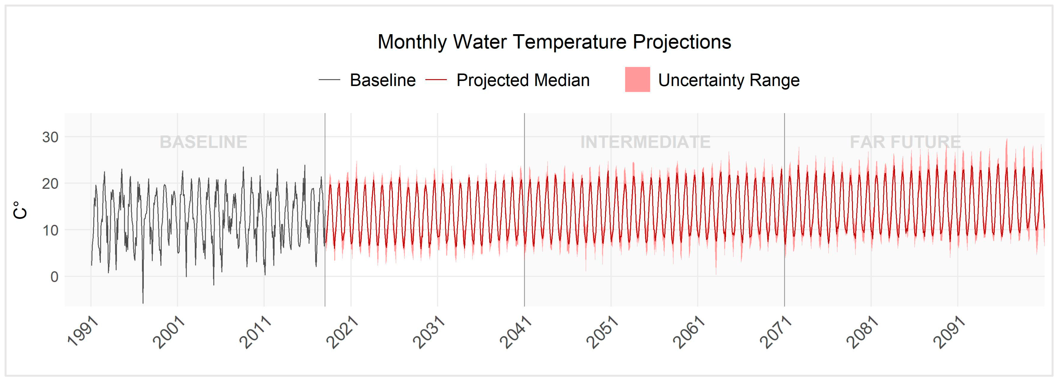
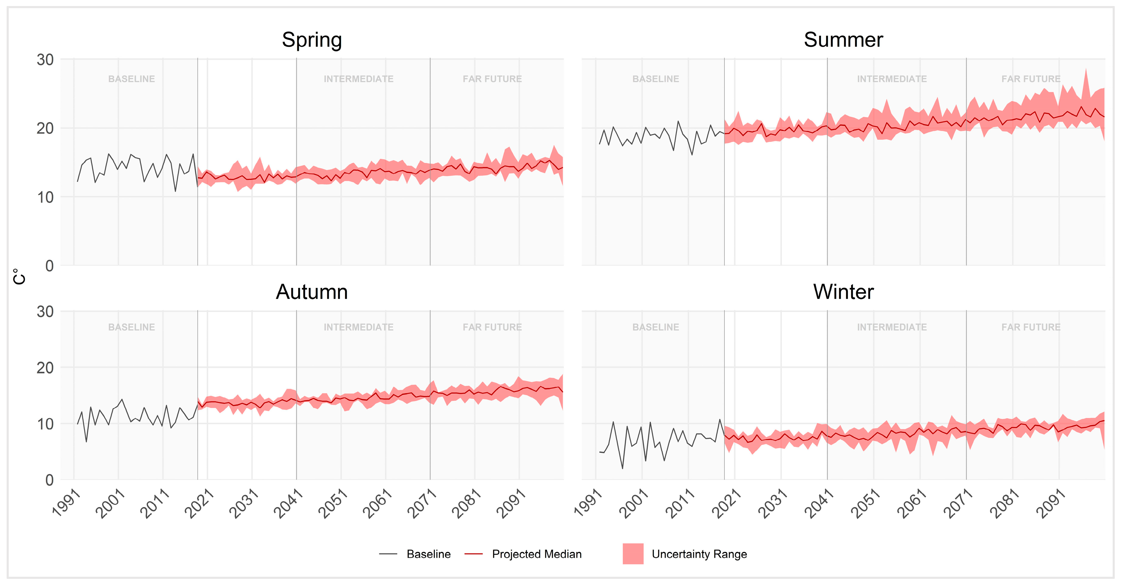
2.3.1. Temporal Analysis of Discharge and Water Temperature

The temporal analysis aimed to evaluate discharge and water temperature trends at the catchment outlet over the modelling period (1991–2100). Discharge was analysed at both daily and monthly scales to assess variability, while water temperature trends were examined using monthly outputs following the SWAT+ default approach [60].

To assess seasonal variability, discharge and water temperature were computed for each year, and seasonal averages were generated. Ensemble-wide statistics were then derived, including the median of the seasonal means, as well as the absolute minimum and maximum values, capturing the full range of potential variability. The median was used for trend analysis to minimize sensitivity to outliers, while the minimum and maximum values represented the upper and lower bounds of projections.

For each time slice, the mean of the median, the minimum of the minima and the maximum of the maxima were calculated, providing a comprehensive assessment of long-term trends and period-based shifts while accounting for uncertainty. By integrating these metrics, the analysis effectively captures gradual climatic trends, seasonal variability and potential extremes in discharge and water temperature dynamics across the Gersprenz catchment.

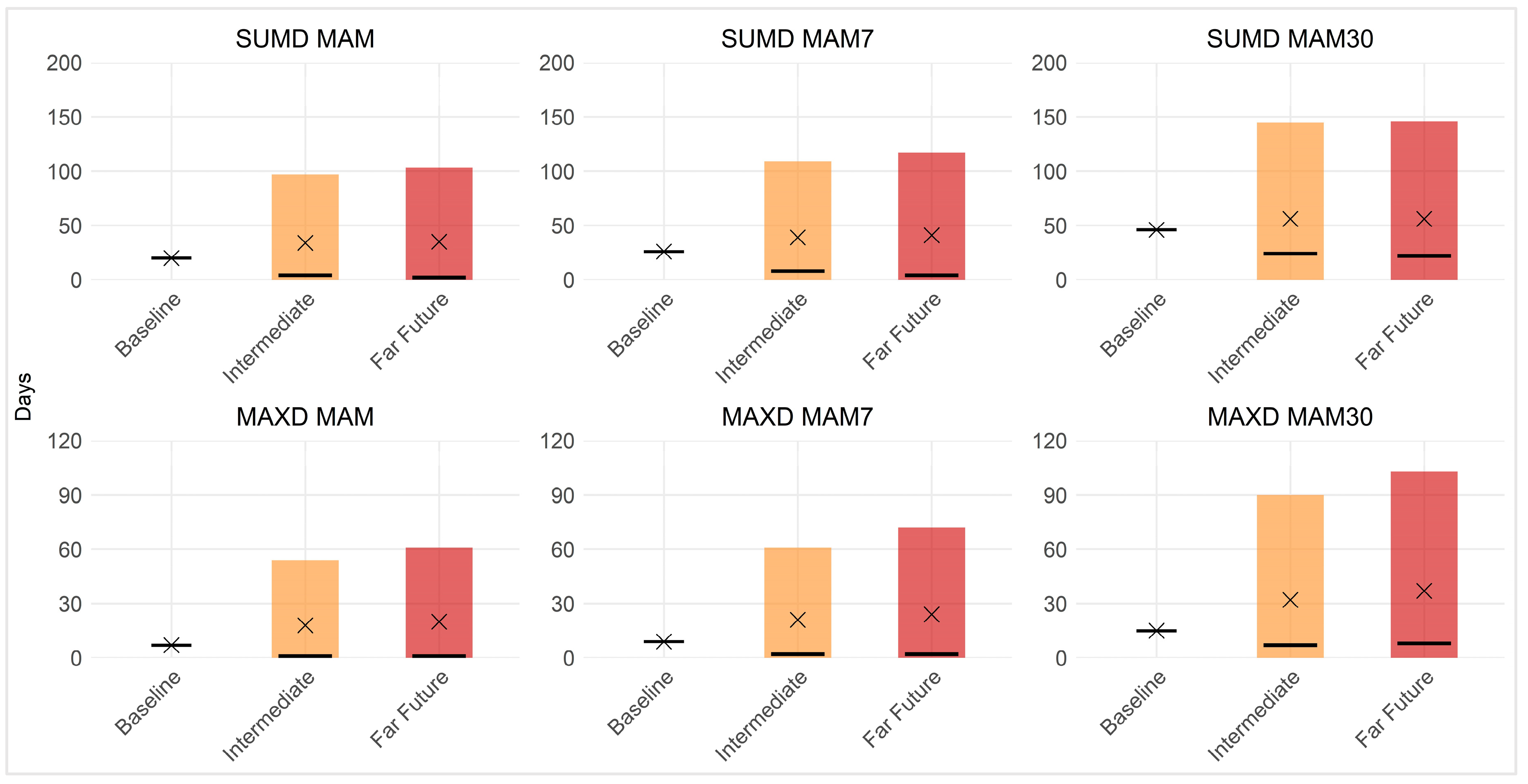
2.3.2. Low Flow Analysis

Low flow conditions were analysed following the methodology outlined by Grosser and Schmalz (2021) evaluating temporal changes in low flow frequency, duration and intensity at the catchment outlet [16].

The lowest daily discharge of each year (AMIN), the lowest weekly discharge of each year (AMIN7) and the lowest monthly discharge of each year (AMIN30) were determined for the entire study period. These metrics provided a detailed assessment of annual low flow behaviour and its progression over time.

To observe projected changes in low flow characteristics, low flow indicators were derived by calculating the mean of the annual minimum time series for the baseline, intermediate and far future. These indicators included mean annual minimum daily discharge (MAM), mean annual minimum weekly discharge (MAM7Q) and mean annual minimum monthly discharge (MAM30Q). In addition, absolute minimum daily flow (AM) and mean annual flow (MQ) were obtained to monitor absolute minimum flow and overall flow trends.

The MAMxQ indicators also serve as thresholds for evaluating the frequency and duration of low flow events. To ensure consistency across time periods, baseline thresholds were uniformly applied to both the intermediate and far future periods. The resulting SUMD represents the total number of days per year with discharge falling below the specified threshold, while MAXD captures the maximum number of consecutive days per year with discharge below that threshold. The annual means of SUMD and MAXD were computed for each time frame and compared to the baseline to assess the evolution of low flow conditions. The full range of ensemble projections was analysed to account for variability and uncertainty, ensuring that both central tendencies and extremes are captured.

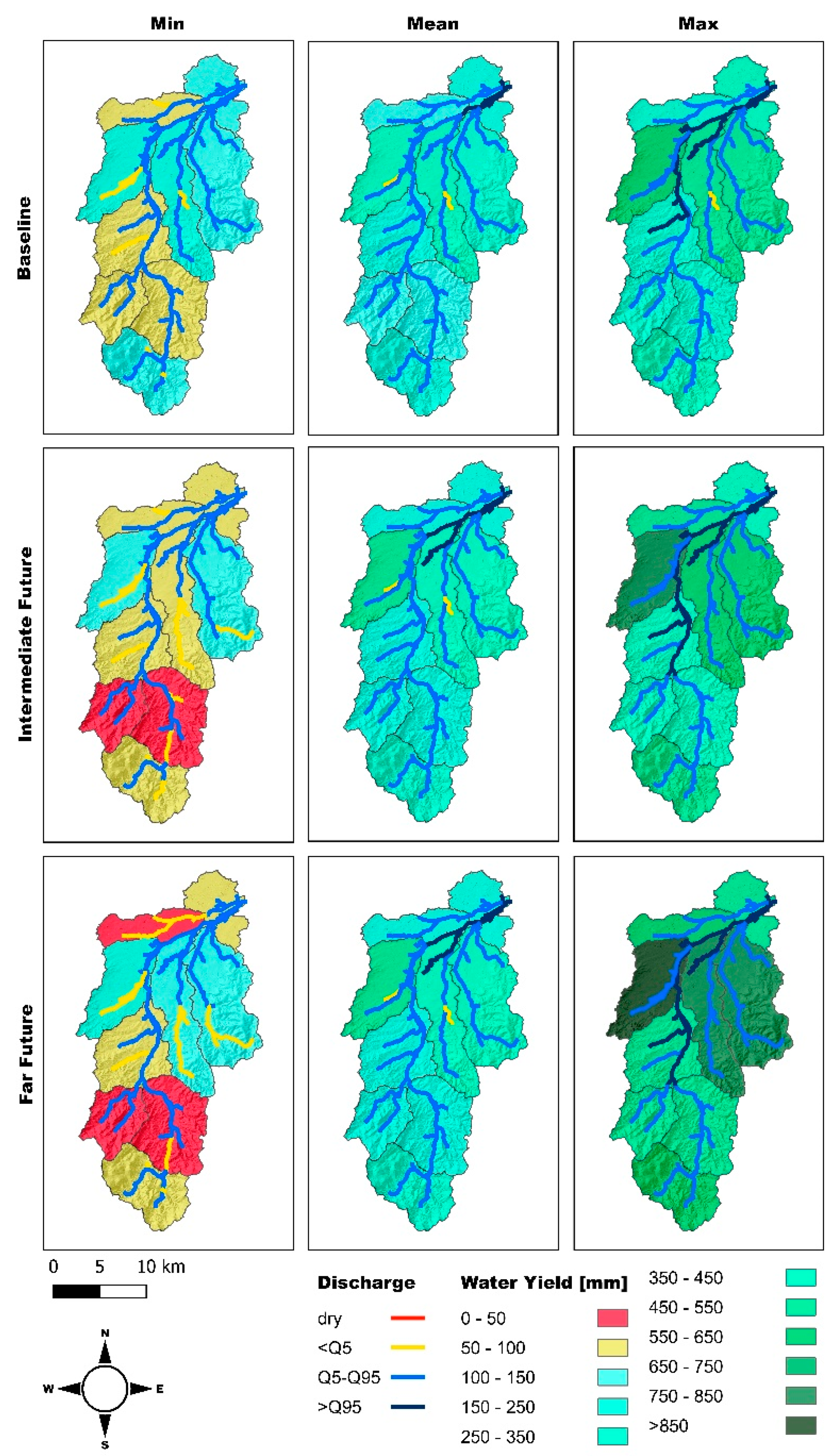
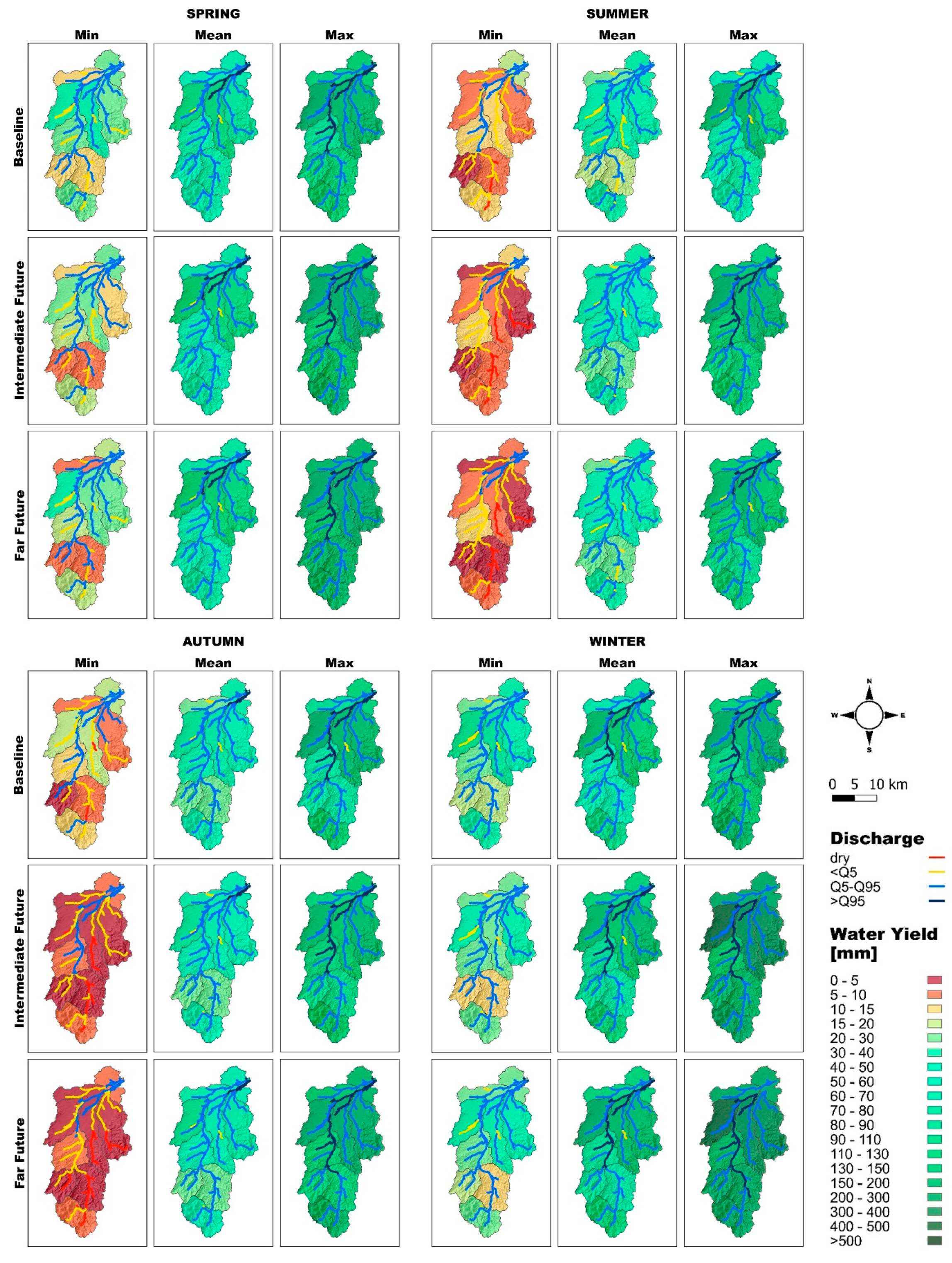
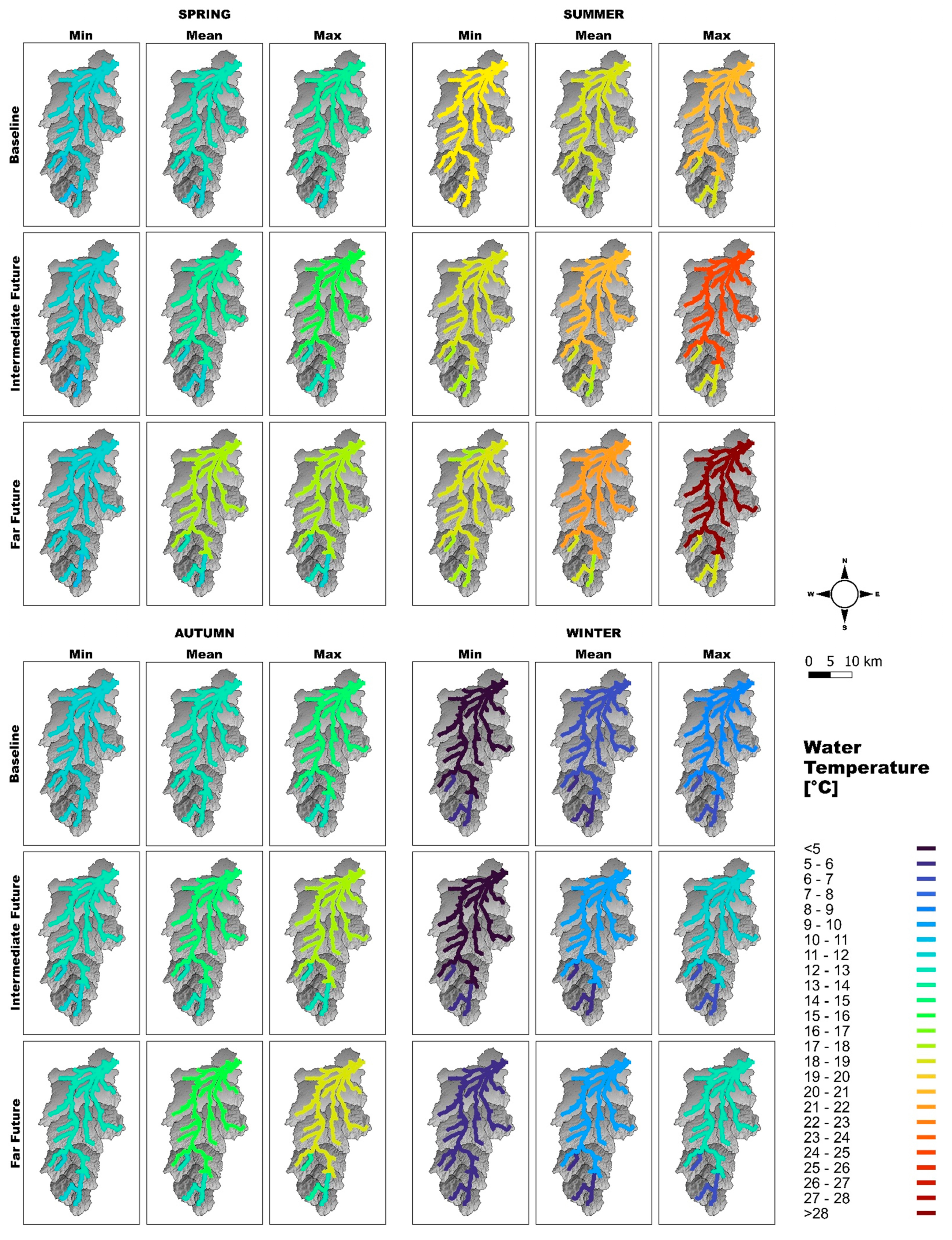
2.3.3. Spatial Analysis of Discharge, Water Yield and Water Temperature

To analyse spatial differences in the development of hydrological variables within the catchment, discharge, water yield and water temperature were assessed at the subcatchment and channel segment levels. The spatial analysis utilized projections from 74 river segments for discharge and in-stream water temperature, while water yield projections were derived by aggregating HRU outputs at the subcatchment level for nine defined subcatchments.

Water yield, a key SWAT+ output variable, represents the total water leaving a sub-basin and contributing to streamflow. It is calculated as the sum of multiple hydrological components [61].

WYLD = SURQ + LATQ + GWQ − TLOSS − pond abstractions

(2)

where:

• SURQ = surface runoff;
• LATQ = lateral flow;
• GWQ = baseflow;
• TLOSS = transmission losses.

The water yield reflects the overall availability of water within a catchment and was utilized in this study as an indicator of water availability.

For the baseline, intermediate and far future periods, absolute minimum, mean and maximum values were determined. An overview of the annual discharge and water yield values was created to capture their temporal development. Seasonal projections for discharge, water yield and water temperature were generated to examine intra-annual variability across the three timeframes.

Spatial maps were generated by integrating SWAT+ text file outputs with geospatial data in QGIS, enabling detailed visualization of regional disparities in hydrological variables. These maps highlight subcatchments and river segments most vulnerable to low flow, water scarcity and extreme thermal conditions. By offering a spatial perspective, the analysis provided critical insights into localized climate change impacts within the Gersprenz catchment.

3. Results

The following results provide a comprehensive analysis of hydrological changes in the Gersprenz catchment under projected future climate conditions for RCP8.5. Temporal trends at the catchment outlet capture overall discharge patterns across monthly, daily and seasonal scales, alongside changes in water temperature. The evolution of low flow conditions is explored using low flow indicators, offering insights into the progression of drought characteristics over time. Finally, a spatial analysis of the discharge, water yield and water temperature highlights regional disparities, identifying subcatchments most vulnerable to low flow conditions and revealing seasonal variations across the basin.

3.1. Temporal Analysis of Discharge and Water Temperature

This section examines the temporal evolution of discharge and water temperature patterns over the entire modelling period, with a focus on monthly and seasonal trends, as well as projected uncertainties under future climate scenarios.

Figure 7 provides an overview of monthly discharges at the outlet of the Gersprenz catchment. While the median monthly discharge remains relatively stable throughout the study period, the widening uncertainty bounds indicate increasing variability and heightened risks of extreme flow conditions, including low flow events.

Daily discharge projections for the intermediate and far future were shown to reinforce this trend, with a growing range of extremes over time. These patterns become more pronounced in the far future, underscoring the potential for more intense and frequent extreme events.

Figure 8 illustrates seasonal discharge projections, highlighting distinct patterns in both discharge levels and variability across seasons. Summer flows are the lowest, while winter discharges are over three times higher on average. Winter also shows the broadest uncertainty range, reflecting a higher potential for extreme high-flow events, whereas summer is characterized by narrower bounds but an elevated risk of low flow extremes. Autumn stands out as a critical season for low flow development, with a marked decline in discharge and minimum discharge values over time. Spring serves as a transitional period with moderate and relatively stable discharge levels.

The seasonal changes become more evident when comparing the development of mean, minimum and maximum discharge values across the baseline, intermediate and far future periods (

Table 8. Seasonal discharge statistics.

	Spring			Summer			Autumn			Winter
	Min	Mean	Max	Min	Mean	Max	Min	Mean	Max	Min	Mean	Max
Baseline	1.54	3.12	6.04	0.70	1.70	3.10	0.93	2.37	6.19	2.14	4.64	8.11
Intermediate	1.35	3.96	7.70	0.36	1.84	7.35	0.44	2.58	6.25	1.97	5.77	11.94
Far Future	1.06	4.19	9.80	0.11	1.64	5.44	0.58	2.66	9.19	2.29	6.39	16.07

). As indicated, mean values change only marginally, whereas the min and max values present more pronounced changes. In summer, the minimum discharge decreases dramatically, dropping from a baseline of 0.70 m³/s to 0.36 m³/s in the intermediate future and further to just 0.11 m³/s in the far future—a decline of about 85% from baseline levels. Similarly, autumn’s minimum discharge falls from 0.93 m³/s to 0.44 m³/s in the intermediate future and 0.58 m³/s in the far future. Minimum discharges in spring decrease from 1.54 m³/s in the baseline to 1.06 m³/s in the far future. Meanwhile, minimum discharges in winter remain more stable and even increase from the baseline to the far future.

Figure 9 presents the temporal evolution of monthly average water temperatures at the catchment outlet. The graph highlights a significant trend of increasing water temperatures over the study period. Seasonal oscillations are evident, the seasonal pattern remaining consistent across the study period, while the amplitude of variation increases as water temperatures rise. This warming trend becomes more pronounced with proceeding time, accompanied by a widening uncertainty range. Towards the end of the century, water temperatures rise by more than 4 °C compared to the baseline, with some ensemble members projecting summer maxima exceeding 28 °C.

Seasonal trends of water temperatures (Figure 10 and

Table 9. Seasonal water temperature statistics.

	Spring			Summer			Autumn			Winter
	Min	Mean	Max	Min	Mean	Max	Min	Mean	Max	Min	Mean	Max
Baseline	10.79	14.30	16.22	16.06	18.70	20.99	6.74	11.17	14.29	2.00	6.94	10.71
Intermediate	11.67	13.43	15.53	18.04	20.30	24.55	12.17	14.51	17.05	4.17	8.18	11.52
Far Future	11.50	14.26	17.53	18.05	21.65	28.75	12.22	15.80	18.87	5.30	9.29	12.13

) reveal that summer and autumn experience the steepest increases in water temperatures. Summer maxima rise by nearly 8 °C in the far future compared to the baseline. Overall increases in mean, minimum and maximum water temperatures are most pronounced in autumn, with mean values rising by 4.63 °C and maximum values by 4.58 °C. Minimum autumn temperatures rise even more steeply, by 5.48 °C, indicating a pronounced warming trend during this season. Winter also shows significant warming, particularly in minimum temperatures, which are projected to increase by 3.3 °C in the far future compared to the baseline. In contrast, changes in spring water temperatures are minimal, with mean temperatures even showing a slight decreasing trend. The minimum and maximum spring temperatures rise modestly by 0.71 °C and 1.31 °C, respectively, in the far future. Overall, the seasonal analysis highlights substantial warming trends, especially in summer and autumn. The widening uncertainty ranges, particularly in summer, underscore the heightened risk of extreme water temperatures under the RCP8.5 scenario.

3.2. Low Flow Analysis

A decline in minimum daily, weekly and monthly discharges was observed with increasing uncertainty over time (Figure 11). While the median remains relatively stable, the lower bound continuously decreases, particularly in the far future, suggesting a growing risk of low flow conditions under extreme conditions.

As shown in

Table 10. Baseline and projected low flow indicators with uncertainty bounds.

		AM	MQ	MAM	MAM7Q	MAM30Q
Baseline		0.279	2.950	0.678	0.748	0.951
Intermediate Future	Min	0.022	1.566	0.294	0.372	0.432
	Mean	0.608	3.670	0.955	1.108	1.337
	Max	0.992	7.420	1.529	1.957	2.708
Far Future	Min	0.097	1.623	0.339	0.388	0.432
	Mean	0.683	3.870	0.964	1.086	1.287
	Max	0.985	7.770	1.495	1.906	2.537

, low flow thresholds themselves shift under climate change. Therefore, to maintain comparability, the baseline thresholds MAM, MAM7Q and MAM30Q were applied also to future periods, allowing for a consistent assessment of low flow characteristics across baseline, intermediate- and far future conditions.

Figure 12 shows the development of the annual total of low flow days (SUMD) and the annual maximum of consecutive low flow days (MAXD) across three thresholds for the baseline, intermediate and far future periods. While the median values of both SUMD and MAXD decrease slightly in both future periods, the mean and maximum values increase significantly, highlighting the intensification of low flow occurrence and duration. Under the threshold MAM30, the annual average of SUMD in the far future peaks at approx. 150 low flow days, while a maximum of approx. 100 consecutive low flow days are projected on average by the ensemble. The ranges, and thus the uncertainty, increase over time and with higher thresholds, with maximum values showing a pronounced upward trend, particularly in the far future.

3.3. Spatial Analysis of Discharge, Water Yield and Water Temperature

Building on the temporal trends observed for the entire catchment, this section examines how projected changes vary spatially across subcatchments and river segments, with a focus on identifying areas most vulnerable to low flow, water scarcity and high stream temperatures.

Figure 13 presents the results of the spatial analysis of annual discharge and water yield across the baseline, intermediate and far future periods. The results indicate that, while the mean annual discharge and water yield remain relatively stable across the Gersprenz River Basin, extreme values intensify over time.

In the baseline period, water yield is relatively homogeneous across subcatchments. However, in the intermediate and far future periods, spatial differences become more pronounced, highlighting subcatchments that are increasingly vulnerable to dry conditions.

Specifically, the upper Gersprenz and the Fischbach subcatchments exhibit annual minimum water yields dropping below 50 mm in the intermediate future, with the Lache subcatchment also falling below this threshold in the far future, indicating an increased vulnerability to hydrological drought in the southern catchments. In contrast, other subcatchments further north appear less impacted by these drying trends. Even in the far future, the minimum annual water yield in these northern subcatchments does not fall below 100 mm. On the contrary, the maximum annual water yield in these areas shows significant increases, with yields exceeding 750 mm in the northeastern subcatchments and peaking over 850 mm in the northwestern subcatchment.

In terms of discharge patterns, the highest discharges occur along the main channel of the Gersprenz, where maximum values often exceed the Q95 threshold. On the other hand, the minimum annual flows are often below the Q5 threshold, especially in the tributaries. This contrast between high and low flows highlights the increasing hydrological variability of the catchment under future climate scenarios. Despite these intensifying extremes, the results indicate that all river reaches will continue to maintain flow throughout the year, with none projected to dry out completely in any given year under future scenarios.

However, while the mean annual flow remains above zero, this does not guarantee continuous flow across all seasons. To better understand both seasonal and spatial variability, seasonal mean flows and water yields were calculated. The mean, minimum and maximum seasonal values were determined for each of the three study periods, incorporating the full range of ensemble data to capture uncertainty. The results are given in Figure 14. The seasonal analysis, based on three-month averages for each season, highlights the varied temporal and spatial impacts of a changing climate on water yield in the Gersprenz catchment. The most pronounced seasonal changes occur in autumn, where minimum water yields show a consistent decline across the entire catchment. In the far future, autumn water yield drops to roughly half of the baseline levels, indicating a significant drying trend. All subcatchments fall below 10 mm in minimum water yield, with seven out of nine subcatchments dropping below 5 mm. In summer, minimum water yields also decline, though with more spatial variability among subcatchments. In the far future, four out of nine subcatchments fall below 5 mm in minimum water yield. As prior in the annual analysis, the subcatchments most affected include the upper Gersprenz, Fischbach and Lache. Even in spring, these three subcatchments remain notably drier than the rest.

Winter shows a slightly different pattern, with a minor increase in overall water yield compared to the baseline period, especially in the northern subcatchments. In particular, the northwestern subcatchment exhibits notably high-water yields, contrasting with the southern subcatchments that continue to experience lower yields.

Several river segments are projected to fall completely dry during the summer and autumn months in future climate scenarios. In the reference period, approximately 3.6% of the river network experiences dry conditions in autumn. However, in the far future, this percentage will increase substantially, with around 25.8% of the river network expected to dry out in autumn. During the summer months, up to 5% of the watercourse can fall dry in the reference period, with this figure rising to 20.3% in the far future, slightly less than in autumn.

The river segments affected by these dry conditions are largely the same in both summer and autumn, suggesting that some sections may experience complete dryness for half of the year in the far future. The affected streams include the Osterbach, Kainsbach, Crumbach, Eberbach, Semme, Taubensemd and Wiebelsbach (Figure 15). Notably, the Fischbach and the Ohlebach are projected to dry out only in autumn but not in summer in the far future. For segments that do not fall completely dry in autumn and summer, seasonal discharge minima nonetheless fall mostly below the Q5 threshold. Only some sections of the main channel maintain flows in the mid-range, highlighting the contrast between tributaries and the main stream. In contrast, spring and winter show more stable discharge patterns, with streams maintaining discharges above zero throughout. Notably, winter projections indicate an increase in high-flow events, with discharge values exceeding the Q95 threshold more frequently, particularly in the main river channels.

As shown in Figure 16, water temperatures show a consistent increase from the baseline to the far future, with maximum temperatures exhibiting the most pronounced warming across all seasons. Summer displays the most pronounced increases, where mean temperatures in the far future rise by 5–8 °C, with maximum temperatures exceeding 28 °C in the central and northern parts of the catchment. In contrast, the southern river segments near the Odenwald springs—including the Fischbach and the Osterbach—remain substantially cooler than the rest of the catchment. On average, these southern segments are 3–4 °C cooler across all seasons compared to the central and northern segments in the far future.

Winter exhibits the smallest temperature increases, with mean water temperatures remaining below 10 °C in the far future, compared to 5–8 °C in the baseline. Mean winter temperatures across the catchment rise by approximately 1–3 °C, with southern regions slightly warmer than northern ones. In spring, mean water temperatures increase to 15–20 °C in the far future, compared to 10–15 °C in the baseline. Maximum spring temperatures approach 25 °C, representing an average increase of 5–6 °C compared to baseline values. Autumn mean temperatures are slightly higher than in spring, rising to 18–22 °C in the far future, compared to 12–16 °C in the baseline. Maximum autumn temperatures increase to 25–28 °C, making autumn the second warmest season after summer. On average, autumn temperatures rise by 6–8 °C, exceeding the increase observed in spring.

4. Discussion

4.1. Discharge and Low Flow

This study projects significant changes in hydrological processes under the RCP8.5 scenario in a representative low mountain range catchment in Germany. The results indicate a strengthening of discharge extremes by the end of the 21st century, with increasingly pronounced low flows, consistent with the trends observed across Hesse [62,63]. The lowest discharge values are projected for the summer months, followed by autumn. In particular, minimum seasonal discharge in summer is expected to decline by 85% compared to the baseline, while autumn sees a 38% decline. Although spring also shows decreased discharge, winter discharges remain stable with even increasing tendencies. These findings align with previous research by Grosser and Schmalz (2023), who reported more frequent and severe droughts in the study region, especially during summer and autumn under RCP8.5 [17]. Their work also observed a tendency toward wetter winters, consistent with both the trends found in this study and observations for Hesse, where summer discharge shifts to winter [64].

In a preceding study, Grosser and Schmalz (2023) analysed far future changes in climate indices relative to the baseline [17]. They documented a fourfold increase in summer hot days (≥30 °C, DWD, 2021) and an eighteenfold increase in autumn [65]. Heat spell durations were projected to rise by a factor of 3 in summer and 22 in autumn, while dry periods without rainfall increased by 31% in summer and 68% in autumn.

While the prior study emphasized more pronounced meteorological changes in autumn, this study finds the lowest discharges during summer with the most significant declines. This underscores the critical role of seasonality, where even minor climatic shifts drastically affect water availability in systems already prone to low flows due to seasonal variations. This vulnerability is particularly evident in rivers and streams that experience minimal discharge in summer as a result of increased evaporation [64]. Additionally, projected hydrological shifts indicate that up to 25.8% of the stream network could experience complete drying during summer and autumn, with smaller tributaries particularly vulnerable. Although summer sees the most severe discharge reductions overall, autumn is projected to have more extensive drying of smaller tributaries, with two additional tributaries ceasing to flow in the long term. This highlights distinct seasonal patterns in low flow dynamics, where summer is marked by the lowest discharge levels, while autumn exhibits a more prolonged and widespread loss of smaller streams, further endangering habitat connectivity and aquatic ecosystems.

The historical trend of decreasing low flow levels in the Gersprenz River identified by Grosser and Schmalz (2021) for 1980–2018 is projected to persist [16]. Projections indicate continued declines in minimum daily, weekly and monthly discharges, with reductions of 48–57% in the intermediate and far future. Severe low flow events are expected to intensify, with absolute minimum daily discharges falling by over 90% and 65% from the baseline. The projected total low flow days (SUMD) may peak at 150 annually, including 100 consecutive days (MAXD), compared to historical averages of 54 and 17 days, respectively. In comparison, in 2018, SUMD was nearly 150 days and MAXD 47 days. The year 2018 was characterized by record-breaking warmth and dryness, with an average temperature of 10.4—2.2 °C above the 1961–1990 reference period [56].

Finally, the projected changes in discharge and low flow indicate substantial alterations in the hydrological regime in the future, with an intensification of low flow conditions, particularly in summer. While greater meteorological changes were projected for autumn [16], the already lower discharge values in summer are expected to decline even further, aligning with investigations by HLNUG that predict a climate-induced intensification of summer low flows [64]. The findings underscore the critical role of seasonality in shaping hydrological processes and provide new insights into the persistent and severe nature of future low flow events in this region.

4.2. Water Temperature

Analysis of future climate conditions in the Gersprenz catchment [17] identified a significant rise in air temperature as the most prominent change, with maximum warming up to 0.8 °C above the German mean. Given the close link between air and water temperatures, this study expanded its focus to include water temperature projections alongside discharge. As air warms, water bodies are affected by heat exchange processes, and low flow conditions worsen these effects by reducing the system’s buffering capacity. This creates a feedback loop: Lower water levels amplify warming, which in turn accelerates evaporation and further reduces discharge [66,67].

The findings reveal a steady increase in water temperatures throughout the 21st century, with all seasons affected, consistent with projections by KLIWA, which highlight a long-term warming trend in river water temperatures in Hesse due to global warming [68]. Autumn shows the highest average increase at 4.63 °C, followed by summer (2.95 °C) and winter (2.35 °C), while spring experiences a modest rise of 0.71 °C. Although autumn has the largest change in seasonal averages, summer is projected to have the greatest increase in maximum seasonal water temperatures. In the far future, summer’s maximum water temperature is expected to exceed 28 °C—nearly 8 °C higher than baseline values. These projections refer specifically to seasonal average water temperatures, providing insight into long-term trends over the 30-year far future period. However, daily maximum water temperatures are expected to increase by a much greater range due to an increase in short-term climatic extremes.

Stream temperature in this study is simulated with SWAT+ using a linear relationship from Stefan and Preud’homme (1993), which calculates water temperature based on air temperature [60]. This method captures the direct influence of air temperature on water temperature—a relationship that becomes increasingly significant under long-term climate change scenarios. Research shows that air temperature is the primary driver of stream temperature changes, accounting for a larger share of increases than other factors [69,70].

Nonetheless, additional factors influence stream temperature, including the mixing of different flow components (e.g., groundwater and surface runoff), heat exchange at the air–water interface and shading by riparian vegetation. Incorporating these processes, as suggested by Peters et al. (2024), could enhance the accuracy of temperature projections [71]. However, given the focus on long-term, climate-induced changes where air temperature is dominant, the decision to use SWAT+’s default approach is justified.

The observed trends raise serious concerns for aquatic ecosystems. Prolonged low flows and rising water temperatures intensify thermal stress, threatening sensitive species and disrupting ecological balance. Elevated temperatures lower oxygen solubility, impairing metabolic functions and compounding low flow effects [72,73,74]. These synergistic stressors highlight the urgent need to understand and mitigate the combined impacts of hydrological and thermal changes on aquatic environments.

4.3. Spatial Analysis

This study examined the spatial patterns of discharge, water yield and water temperature over time to analyse subcatchment dynamics under climate change. The results reveal areas that are vulnerable to low flow, water scarcity and high water temperatures, as well as regions that exhibit greater resilience.

4.3.1. Southern Subcatchments

Subcatchments in the southern part of the basin, including the upper Gersprenz and Fischbach, consistently show the lowest projected water yields. In both the intermediate and far future, these areas are expected to face severe water deficits, with annual minimum water yields falling below 50 mm. Seasonally, autumn is the most critical period, with water yields dropping to half of baseline levels across the catchment. Similarly, summer experiences significant declines, with over half of the subcatchments falling below 5 mm in minimum water yield by the far future. The most severe drying trends occur in these southern areas, increasing hydrological stress.

Uniform Q5 and Q95 thresholds, applied across the entire basin and determined at the catchment outlet, mean that smaller headwater streams in the south are more likely to fall below the Q5 threshold due to their lower baseline discharges. However, the prolonged drying of tributaries reflects genuine hydrological shifts rather than just methodological constraints. River segments projected to dry out during summer and autumn could represent up to 25.8% of the stream network by the far future. Smaller tributaries are especially at risk, with some segments expected to remain dry for extended periods, posing serious threats to habitat connectivity and aquatic ecosystems.

In terms of water temperature, summer maximums exceeding 28 °C are projected for central and northern river segments, which poses risks to temperature-sensitive species. Interestingly, despite the lower water yields in the southern subcatchments, areas near the Odenwald springs maintain water temperatures that are on average 3–4 °C cooler than those in central and northern segments throughout all seasons in the far future. This cooling effect is attributed to the influence of groundwater-fed springs, which offer a consistent, cooler water supply. However, while these areas act as thermal refuges, their low water volumes restrict habitat capacity.

4.3.2. Northern Subcatchments

In contrast, most northern subcatchments in the downstream region exhibit greater resilience, maintaining water yields above 100 mm, with some areas even experiencing increases. However, despite generally higher water availability, smaller tributaries like the Wiebelsbach are still projected to dry out during summer and autumn. This is likely due to localized hydrological constraints, such as shallow groundwater reserves, low baseflow contributions and increased seasonal evapotranspiration, making them particularly vulnerable to extended dry periods.

An exception to the general high water yields of the northern subcatchments is the northern Lache catchment, where minimum annual water yields are projected to fall below 50 mm in the far future, indicating significant water stress and potential hydrological instability.

The differences in water yield between the southern and northern parts of the catchment can be attributed to geological and hydrological sub-basin characteristics. The southern region is dominated by coarse-grained substrates with low water retention capacity—consisting of granite, diorite and other silicate-rich crystalline rocks [75]—leading to quick runoff and reduced long-term retention. In contrast, the northern catchment transitions into the Reinheimer Hill Country and the Lower Main Plain, where sand, gravel and clay create softer rock soils that enhance infiltration and storage [22]. A larger porous aquifer system in the north provides greater groundwater storage and sustained baseflow [76,77].

Seasonally, winter offers a modest increase in overall water yield and more frequent high-flow events (exceeding the Q95 threshold), particularly in main river channels. However, this seasonal compensation does not fully compensate for the significant deficits observed during summer and autumn.

Key findings reveal significant spatial and seasonal variability in the Gersprenz catchment’s climate change response. Southern subcatchments show persistent low yields and vulnerability in summer and autumn, while northern areas, though having higher yields, face elevated temperatures. Southern thermal refuges underscore the need for targeted water management and conservation measures. This variability highlights the need for targeted water management strategies to address distinct challenges across the catchment.

4.4. Uncertainties and Limitations

As with any climate change impact assessment, this study is subject to inherent uncertainties arising from climate scenario selection, model simplifications and assumptions regarding future conditions. These uncertainties must be considered when interpreting the results and their implications for hydrological planning and management.

A key limitation of this study is the reliance on a single climate scenario (RCP8.5). This choice was based, among other factors, on prior findings by Grosser and Schmalz (2023), which indicated that climatic changes under RCP2.6 were largely marginal for the study region [17]. Additionally, RCP8.5 serves as an upper-bound scenario, providing a worst-case framework for preparedness and adaptive management strategies. While Shared Socioeconomic Pathways offer a broader range of potential future trajectories, this study opted for bias-adjusted and regionalized climate data from the German Weather Service (DWD) to ensure sufficient spatial resolution, accuracy and comparability with previous research. Furthermore, with global temperatures already surpassing the 1.5 °C threshold, the feasibility of achieving RCP2.6’s low-emission pathway is becoming increasingly unlikely [57,78].

This approach aligns with recommendations from KLIWA, which emphasize that observed temperature trends already exceed the projections of many climate models. Given this trend, the necessity of considering the full range of climate projections in impact assessments, with a particular emphasis on worst-case scenarios for risk evaluation is highlighted [79].

The range of possible future outcomes under RCP8.5 was accounted for by analysing the full spectrum of projection results, including upper and lower bounds, rather than focusing solely on mean and median values, which primarily represent central tendencies and may not fully capture the extent of variability or extreme events. This approach ensures a more comprehensive assessment of extreme conditions, which is essential for preparedness planning.

Additionally, hydrological models, including SWAT+, are simplifications of real-world processes and can only partially capture the complex and escalating effects of climate change. Despite SWAT+ being a detailed process-based model, certain simplifications were necessary within this study. For instance, groundwater processes are represented conceptually, and although key aquifer parameters were calibrated, the model does not simulate spatial groundwater table dynamics or lateral aquifer interactions. This may limit the accuracy of baseflow representation in areas with complex hydrogeology. Similarly, land use management was simplified to a basic crop rotation to maintain focus on climate-driven hydrological changes. Moreover, only temperature and precipitation projections were incorporated, while other potentially relevant climate variables (e.g., solar radiation, humidity and wind speed) were excluded to isolate the effects of the primary drivers of low flow and drought conditions.

Furthermore, land use change was not considered in the scenario modelling process. While an analysis of CORINE land cover data by Grosser and Schmalz (2021) indicated that sealed areas increased by only ~2% between 1990 and 2018, the extent of future land-use transformations remains uncertain [16]. Changes such as increased urbanization, afforestation or agricultural intensification can substantially influence key hydrological processes, including runoff generation, infiltration capacity and ultimately low flow behaviour. While this study was designed to isolate the effects of climatic drivers, incorporating land use change scenarios in future research would allow for a more comprehensive assessment of potential hydrological responses by accounting for an additional important driver of change.

In addition, changes in atmospheric CO₂ concentrations were not accounted for directly within the SWAT+ model. While CO₂ is inherently reflected in the climate projections used under RCP8.5, potential physiological feedback of elevated CO₂ on plant growth and evapotranspiration were not considered. Incorporating CO₂-related vegetation responses in future studies could further improve process representation, particularly in assessments where dynamic vegetation feedback may play a significant role under changing climate conditions.

Despite inherent uncertainties, this study provides a baseline for future hydrological developments, offering insights into climate change impacts on water availability across spatial and temporal scales. While projection uncertainty increases over time due to interacting global drivers, the resulting outcome range itself serves as a valuable basis for adaptive planning. The scenario-based approach enables a structured assessment of climate-induced risks under a defined forcing pathway and remains transferable to similar contexts. By isolating climate as the primary driver, the simulated changes are primarily attributable to climatic forcing, while acknowledging that future hydrological conditions may also be affected by socioeconomic developments not considered in this study.

5. Summary and Conclusions

This study provides a comprehensive assessment of future hydrological dynamics in the German Gersprenz catchment under the RCP8.5 scenario, including projections of streamflow with an emphasis on low flow conditions, water yield and water temperature, analysed across multiple spatial and temporal scales, addressing three key research questions.

Firstly, with respect to seasonal streamflow dynamics and long-term trends, projections indicate a substantial intensification of discharge extremes by the late 21st century. Minimum seasonal discharges are expected to decline by up to 85% in summer and 38% in autumn relative to baseline conditions (1991–2017), while winter flows may remain stable or potentially increase. Although overall low flow conditions are most pronounced in summer, driven by the greatest reductions in discharge, the long-term desiccation of smaller tributaries is more evident in autumn. Enhanced evapotranspiration during summer intensifies water loss and depletes soil moisture, thereby reinforcing a feedback mechanism that prolongs low flow events and may extend their duration to up to 150 days annually. In contrast, in autumn, persistent hydrological deficits contribute to the progressive drying of smaller tributaries, emphasizing seasonal variations in low flow responses. These findings highlight the critical role of seasonality, demonstrating that even minor climatic shifts can significantly alter water availability in already water-stressed systems.

Second, rising air temperatures will have a direct impact on water temperatures, with a consistent warming trend projected across all seasons. Summer maximum water temperatures are expected to exceed 28 °C—an increase of nearly 8 °C compared to baseline values—posing significant thermal stress on aquatic ecosystems. Elevated water temperatures reduce oxygen solubility, disrupt physiological processes and impair metabolic functions in temperature-sensitive species, thereby intensifying ecological stress and potentially altering ecosystem stability.

Third, spatial analysis reveals substantial subcatchment scale variability in hydrological responses and thermal dynamics. In the southern catchment, where coarse-grained crystalline substrates with low water retention dominate, persistent low water yields and severe drying trends are projected for summer and autumn. Despite these conditions, groundwater-fed springs provide critical thermal refuges, maintaining water temperatures 3–4 °C lower than in central and northern areas, though their limited water volumes constrain their buffering capacity. In contrast, northern subcatchments, characterized by higher infiltration capacities and a more extensive aquifer system, generally sustain greater water yields, though localized stress still occurs.

These findings highlight the pronounced spatial and seasonal heterogeneity in the catchment’s climate response, emphasizing emerging hotspots of water stress across different subcatchments and time periods. While groundwater-fed springs provide localized cooling, their limited discharge restricts habitat availability. Northern subcatchments, despite higher water yields, remain vulnerable to rising temperatures and seasonal local low flow extremes, particularly in summer and autumn. The findings emphasize that even regions with sufficient annual water yields may develop acute seasonal and spatial water stress, in response to rising temperatures and changing precipitation patterns. Furthermore, they highlight how seasonality and catchment characteristics drive hydrological responses, underscoring the need for subcatchment scale management to address localized vulnerabilities and seasonal water deficits.

Finally, this study offers insights applicable to catchments experiencing spatially or temporally localized water stress, presenting a scalable methodology that informs climate adaptation strategies and sustainable water management. By integrating a process-based hydrological model with bias-corrected climate projections under RCP8.5 as an upper-range scenario for preparedness, it captures long-term hydrological trends, intra-annual seasonal variability and spatial heterogeneity, enabling an assessment of climate-induced hydrological stress at the subcatchment level. Additionally, by incorporating the full range of ensemble projections, this study ensures a comprehensive evaluation of potential hydrological changes, supporting robust adaptation planning. The incorporation of extreme low flow metrics and spatially resolved projections of water yield, temperature and discharge enhances this analysis, providing a transferable framework for identifying spatio-temporal hotspots of water stress in river basins. This approach delivers actionable data for targeted adaptation strategies, enabling decision-makers to implement measures where they are most needed.

References

1. Abbas, M.; Zhao, L.; Wang, Y. Perspective Impact on Water Environment and Hydrological Regime Owing to Climate Change: A Review. Hydrology 2022, 9, 203. [Google Scholar] [CrossRef]
2. Cao, Z.; Wang, S.; Luo, P.; Xie, D.; Zhu, W. Watershed Ecohydrological Processes in a Changing Environment: Opportunities and Challenges. Water 2022, 14, 1502. [Google Scholar] [CrossRef]
3. Chaturvedi, A.; Pandey, B.; Yadav, A.K.; Saroj, S. An Overview of the Potential Impacts of Global Climate Change on Water Resources. In Water Conservation in the Era of Global Climate Change; Elsevier: Amsterdam, The Netherlands, 2021; pp. 99–120. ISBN 978-0-12-820200-5. [Google Scholar]
4. Sohoulande Djebou, D.C.; Singh, V.P. Impact of Climate Change on the Hydrologic Cycle and Implications for Society. Environ. Soc. Psychol. 2016, 1, 36–49. [Google Scholar] [CrossRef]
5. Schneider, C.; Laizé, C.L.R.; Acreman, M.C.; Flörke, M. How Will Climate Change Modify River Flow Regimes in Europe? Hydrol. Earth Syst. Sci. 2013, 17, 325–339. [Google Scholar] [CrossRef]
6. Christensen, J.H.; Hewitson, B.; Busuioc, A.; Chen, A.; Gao, X.; Held, I.; Jones, R.; Kolli, R.; Kwon, W.; Laprise, R.; et al. Regional Climate Projections. In Climate Change 2007: The Physical Science Basis. Contribution of Working Group I to the Fourth Assessment Report of the Intergovernmental Panel on Climate Change; 2007; Available online: https://www.ipcc.ch/report/ar4/wg1/ (accessed on 4 March 2025).
7. Alcamo, J.; Flörke, M.; Märker, M. Future Long-Term Changes in Global Water Resources Driven by Socio-Economic and Climatic Changes. Hydrol. Sci. J. 2007, 52, 247–275. [Google Scholar] [CrossRef]
8. Riedel, T.; Nolte, C.; aus der Beek, T.; Liedtke, J.; Sures, B.; Grabner, D. Niedrigwasser, Dürre und Grundwasserneubildung—Bestandsaufnahme zur gegenwärtigen Situation in Deutschland, den Klimaprojektionen und den existierenden Maßnahmen und Strategien; German Environment Agency: Dessau-Roßlau, Germany, 2021. [Google Scholar]
9. BUND Auswirkungen des Klimawandels auf den Wasserhaushalt. Ein Hintergrunddossier zu den Auswirkungen des Klimawandels auf den Zustand und die Gefährdung der Gewässer in Deutschland und die Folgen für die Nutzungen. BUND-Gewässerpapier 2020. Available online: https://digital.zlb.de/viewer/metadata/34758580/1/ (accessed on 4 March 2025).
10. Brienen, S.; Walter, A.; Brendel, C.; Fleischer, C.; Ganske, A.; Haller, M.; Helms, M.; Höpp, S.; Jensen, C.; Jochumsen, K.; et al. Klimawandelbedingte Änderungen in Atmosphäre Und Hydrosphäre: Schlussbericht Des Schwerpunktthemas Szenarienbildung (SP-101) Im Themenfeld 1 Des BMVI-Expertennetzwerks. 2020, p. 157. Available online: https://www.bmdv-expertennetzwerk.bund.de/DE/Publikationen/TFSPTBerichte/SPT101.html (accessed on 4 March 2025).
11. Flörke, M.; Uschan, T.; Stein, U.; Tröltzsch, J.; Vidaurre, R.; Schritt, H.; Bueb, B.; Reineke, J.; Herrmann, F.; Kollet, S.; et al. Auswirkung des Klimawandels auf die Wasserverfügbarkeit. Anpassung an Trockenheit und Dürre in Deutschland (WAD-Klim). 2024. Available online: https://www.umweltbundesamt.de/publikationen/auswirkung-des-klimawandels-auf-die (accessed on 4 March 2025).
12. German Environment Agency. Interministerial Working Group on Adaptation to Climate Change 2023 Monitoring Report on the German Strategy for Adaptation to Climate Change; German Environment Agency: Dessau-Roßlau, Germany, 2023. [Google Scholar]
13. David, A.; Schmalz, B. Flood Hazard Analysis in Small Catchments: Comparison of Hydrological and Hydrodynamic Approaches by the Use of Direct Rainfall. J. Flood Risk Manag. 2020, 13, e12639. [Google Scholar] [CrossRef]
14. David, A.; Schmalz, B. A Systematic Analysis of the Interaction Between Rain-on-Grid-Simulations and Spatial Resolution in 2D Hydrodynamic Modeling. Water 2021, 13, 2346. [Google Scholar] [CrossRef]
15. David, A.; Rodriguez, E.R.; Schmalz, B. Importance of Catchment Hydrological Processes and Calibration of Hydrological-hydrodynamic Rainfall-runoff Models in Small Rural Catchments. J. Flood Risk Manag. 2023, 16, e12901. [Google Scholar] [CrossRef]
16. Grosser, P.F.; Schmalz, B. Low Flow and Drought in a German Low Mountain Range Basin. Water 2021, 13, 316. [Google Scholar] [CrossRef]
17. Grosser, P.F.; Schmalz, B. Projecting Hydroclimatic Extremes: Climate Change Impacts on Drought in a German Low Mountain Range Catchment. Atmosphere 2023, 14, 1203. [Google Scholar] [CrossRef]
18. Grosser, P.F.; Xia, Z.; Alt, J.; Rüppel, U.; Schmalz, B. Virtual Field Trips in Hydrological Field Laboratories: The Potential of Virtual Reality for Conveying Hydrological Engineering Content. Educ. Inf. Technol. 2023, 28, 6977–7003. [Google Scholar] [CrossRef]
19. Kissel, M.; Schmalz, B. Comparison of Baseflow Separation Methods in the German Low Mountain Range. Water 2020, 12, 1740. [Google Scholar] [CrossRef]
20. Kissel, M.; Bach, M.; Schmalz, B. Evaluation of Baseflow Modeling with BlueM.Sim for Long-Term Hydrological Studies in the German Low Mountain Range of Hesse, Germany. Hydrology 2023, 10, 222. [Google Scholar] [CrossRef]
21. Kissel, M.; Bach, M.; Schmalz, B. Impact of the Model Structure and Calibration Strategy on Baseflow Modeling in the German Low Mountain Range. J. Hydroinform. 2024, 26, 1692–1714. [Google Scholar] [CrossRef]
22. Schmalz, B.; Kruse, M. Impact of Land Use on Stream Water Quality in the German Low Mountain Range Basin Gersprenz. Landsc. Online 2019, 72, 1–17. [Google Scholar] [CrossRef]
23. Scholand, D.; Schmalz, B. Deriving the Main Cultivation Direction from Open Remote Sensing Data to Determine the Support Practice Measure Contouring. Land 2021, 10, 1279. [Google Scholar] [CrossRef]
24. Scholand, D.; Schmalz, B. Automated Quantification of Contouring as Support Practice for Improved Soil Erosion Estimation Considering Ridges. Int. Soil Water Conserv. Res. 2024, 12, 761–774. [Google Scholar] [CrossRef]
25. Bieger, K.; Arnold, J.G.; Rathjens, H.; White, M.J.; Bosch, D.D.; Allen, P.M.; Volk, M.; Srinivasan, R. Introduction to SWAT+, A Completely Restructured Version of the Soil and Water Assessment Tool. JAWRA J. Am. Water Resour. Assoc. 2017, 53, 115–130. [Google Scholar] [CrossRef]
26. Riahi, K.; Rao, S.; Krey, V.; Cho, C.; Chirkov, V.; Fischer, G.; Kindermann, G.; Nakicenovic, N.; Rafaj, P. RCP 8.5—A Scenario of Comparatively High Greenhouse Gas Emissions. Clim. Change. 2011, 109, 33–57. [Google Scholar] [CrossRef]
27. IPCC 5th Assessment Synthesis Report: Summary for Policymakers. Available online: http://ar5-syr.ipcc.ch/topic_summary.php (accessed on 4 March 2025).
28. Ihwb Feldlabor. Available online: https://www.ihwb.tu-darmstadt.de/forschung_ihwb/feldlabor_ihwb/index.de.jsp (accessed on 25 April 2025).
29. CDC Climate Data Center. Available online: https://www.dwd.de/EN/climate_environment/cdc/cdc_node_en.html (accessed on 3 March 2025).
30. HVBG Geodaten Online—Downloadcenter. Available online: https://gds.hessen.de/INTERSHOP/web/WFS/HLBG-Geodaten-Site/de_DE/-/EUR/ViewDownloadcenter-Start (accessed on 3 March 2025).
31. AdV (Arbeitsgemeinschaft der Vermessungsverwaltungen der Länder der Bundesrepublik Deutschland) Amtliches Topographisch-Kartographisches Informationssystem (ATKIS). Available online: https://www.adv-online.de/AdV-Produkte/Geotopographie/ATKIS/ (accessed on 4 March 2025).
32. BKG Bundesamt Für Kartographie Und Geodäsie. Available online: https://gdz.bkg.bund.de/index.php/default/open-data/corine-land-cover-5-ha-stand-2018-clc5-2018.html (accessed on 3 March 2025).
33. HLNUG INSPIRE ATOM Feed Client. Available online: https://www.geoportal.hessen.de/mapbender/plugins/mb_downloadFeedClient.php?url=https%3A%2F%2Fwww.geoportal.hessen.de%2Fmapbender%2F%2Fphp%2Fmod_inspireDownloadFeed.php%3Fid%3De4e7e5a4-d53a-91b4-b68f-4086986d483e%26type%3DSERVICE%26generateFrom%3Dmetadata (accessed on 3 March 2025).
34. HLNUG: Hessisches Landesamt für Naturschutz, Umwelt und Geologie. Discharge Data of the Gauges Harreshausen (ID: 24762653) and Groß Bieberau 2 (ID: 24761005); HLNUG: Wiesbaden, Germany, 2019. [Google Scholar]
35. Destatis Land-Und Forstwirtschaft, Fischerei. Wachstum Und Ernte–Feldfrüchte–Fachserie 3 Reihe 3.2. Destatis Land-Und Forstwirtschaft, Fischerei: 2022. Available online: https://www.destatis.de/DE/Themen/Branchen-Unternehmen/Landwirtschaft-Forstwirtschaft-Fischerei/_inhalt.html (accessed on 4 March 2025).
36. Achilles, W.; Anter, J.; Belau, T.; Blankenburg, J. Faustzahlen für die Landwirtschaft; 15. Auflage.; Kuratorium für Technik und Bauwesen in der Landwirtschaft e.V. (KTBL): Darmstadt, Germany, 2018; ISBN 978-3-945088-59-3. [Google Scholar]
37. Clementini, C.; Pomente, A.; Latini, D.; Kanamaru, H.; Vuolo, M.R.; Heureux, A.; Fujisawa, M.; Schiavon, G.; Del Frate, F. Long-Term Grass Biomass Estimation of Pastures from Satellite Data. Remote Sens. 2020, 12, 2160. [Google Scholar] [CrossRef]
38. BMEL Dritte Bundeswaldinventur. Available online: https://www.bundeswaldinventur.de/ (accessed on 3 March 2025).
39. Encyclopædia Britannica Understanding Biomass in Forests. Available online: https://www.britannica.com/video/152193/biomass-forests (accessed on 3 March 2025).
40. HessenForst Hesse–A Forest State. Available online: https://www.hessen-forst.de/ueber-den-landesbetrieb-hessenforst/hessenforst-sustainable-forest-management-engl (accessed on 3 March 2025).
41. Katzenmaier D, Fritsch U, Bronstert A. 2001. Quantifizierung des Einflusses von Landnutzung und dezentraler Versickerung auf die Hochwasserentstehung. In Hochwasserschutz heute–Nachhaltiges Management; Heiden, S., Erb, R., Sieker, F., Eds.; Erich Schmidt Verlag: Berlin, Germany, 2001; pp. 327–357. [Google Scholar]
42. Forst Erklärt Unsere Bäume—Die Rotbuche (Fagus Sylvatica). 2020. Available online: https://forsterklaert.de/die-rotbuche (accessed on 4 March 2025).
43. Fleck, S.; Ahrends, B.; Meesenburg, H. Trockenstressrisiko Im Harz. AFZ-DerWald. 2022. Available online: https://www.digitalmagazin.de/marken/afz-derwald/hauptheft/2022-15/waldokologie/021_trockenstressrisiko-im-harz (accessed on 4 March 2025).
44. Deutsche Welle Natur Und Umwelt, Wiederauferstehung Einer Waldlandschaft. Available online: https://www.dw.com/de/wiederauferstehung-einer-waldlandschaft/a-37104507 (accessed on 3 March 2025).
45. Morris, M.D. Factorial Sampling Plans for Preliminary Computational Experiments. Technometrics 1991, 33, 161–174. [Google Scholar] [CrossRef]
46. Van Griensven, A.; Meixner, T.; Grunwald, S.; Bishop, T.; Diluzio, M.; Srinivasan, R. A Global Sensitivity Analysis Tool for the Parameters of Multi-Variable Catchment Models. J. Hydrol. 2006, 324, 10–23. [Google Scholar] [CrossRef]
47. Schuerz, C. SWATplusR. 2022. Available online: https://scholar.google.com/scholar?q=Schuerz%2C%20C.%20(2022).%20Getting%20started%20with%20SWATplusR%20%E2%80%A2%20SWATplusR (accessed on 4 March 2025).
48. Chawanda, C. SWAT+ Toolbox; 2022. Available online: http://openwater.network/assets/downloads/SWATPlusToolboxv0.5.0Installer.exe (accessed on 4 March 2025).
49. Gupta, H.V.; Sorooshian, S.; Yapo, P.O. Status of Automatic Calibration for Hydrologic Models: Comparison with Multilevel Expert Calibration. J. Hydrol. Eng. 1999, 4, 135–143. [Google Scholar] [CrossRef]
50. Moriasi, D.N.; Arnold, J.G.; Liew, M.W.V.; Bingner, R.L.; Harmel, R.D.; Veith, T.L. Model Evaluation Guidelines for Systematic Quantification of Accuracy in Watershed Simulations. Trans. ASABE 2007, 50, 885–900. [Google Scholar] [CrossRef]
51. Knoben, W.J.M.; Freer, J.E.; Woods, R.A. Technical Note: Inherent Benchmark or Not? Comparing Nash–Sutcliffe and Kling–Gupta Efficiency Scores. Hydrol. Earth Syst. Sci. 2019, 23, 4323–4331. [Google Scholar] [CrossRef]
52. Gupta, H.V.; Kling, H.; Yilmaz, K.K.; Martinez, G.F. Decomposition of the Mean Squared Error and NSE Performance Criteria: Implications for Improving Hydrological Modelling. J. Hydrol. 2009, 377, 80–91. [Google Scholar] [CrossRef]
53. Krähenmann, S.; Walter, A.; Klippel, L.; Statistische Aufbereitung Von Klimaprojektionen: Downscaling Und Multivariate Bias-Adjustierung—Im Rahmen Des BMVI-Expertennetzwerkes Entwickelte Verfahren Zum Postprocessing Von Klimamodelldaten. Berichte Des Deutschen Wetterdienstes 254. Available online: https://refubium.fu-berlin.de/handle/fub188/33572 (accessed on 4 March 2025).
54. Krähenmann, S.; Haller, M.; Walter, A. A New Combined Statistical Method for Bias Adjustment and Downscaling Making Use of Multi-Variate Bias Adjustment and PCA-Driven Rescaling. Meteorol. Z. 2021, 30, 391–411. [Google Scholar] [CrossRef]
55. Dalelane, C.; Früh, B.; Steger, C.; Walter, A. A Pragmatic Approach to Build a Reduced Regional Climate Projection Ensemble for Germany Using the EURO-CORDEX 8.5 Ensemble. J. Appl. Meteorol. Clim. 2018, 57, 477–491. [Google Scholar] [CrossRef]
56. DWD Deutscher Wetterdienst. Available online: https://www.dwd.de/ref-ensemble (accessed on 4 March 2025).
57. Shukla, P.R.; Skea, J.; Slade, R.; Al Khourdajie, A.; van Diemen, R.; McCollum, D.; Pathak, M.; Some, S.; Vyas, P.; Fradera, R.; et al. (Eds.) Climate Change 2022: Impacts, Adaptation and Vulnerability. Contribution of Working Group III to the Sixth Assessment Report of the Intergovernmental Panel on Climate Change; 2022; ISBN 978-92-9169-160-9. Available online: https://www.ipcc.ch/report/ar6/wg2/ (accessed on 4 March 2025).
58. Kreienkamp, F.; Huebener, H.; Linke, C.; Spekat, A. Good Practice for the Usage of Climate Model Simulation Results–a Discussion Paper. Environ. Syst. Res. 2012, 1, 9. [Google Scholar] [CrossRef]
59. WMO Guide to Climatological Practices. In Technical Report, World Meteorological Organization, (WMO-No. 100), 3rd ed.; World Meteorological Organization: Geneva, Switzerland, 2010.
60. Stefan, H.G.; Preud’homme, E.B. Stream Temperature Estimation from Air Temperature. JAWRA J. Am. Water Resour. Assoc. 1993, 29, 27–45. [Google Scholar] [CrossRef]
61. Neitsch, S.L.; Arnold, J.G.; Kiniry, J.R.; Williams, J.R. Soil and Water Assessment Tool Theoretical Documentation Version 2009. 2011. Available online: https://oaktrust.library.tamu.edu/items/ee261b66-c392-40d9-8c03-e455f5a8347e (accessed on 4 March 2025).
62. KLIWA 7. In KLIWA Symposium. Zu Wenig|Zu Viel—Wasserwirtschaft Zwischen Trockenheit Und Starkregen; 2023; Available online: https://zentrum-klimaanpassung.de/vernetzung-veranstaltungen/termine/zu-wenig-zu-viel-wasserwirtschaft-zwischen-trockenheit-und-starkregen (accessed on 4 March 2025).
63. Brahmer, G.; Wrede, S. Auswirkungen Des Klimawandels Auf Die Abflussver Hältnisse an Hessischen Flüssen Auf Basis Hochaufgelöster Klima- Und Wasserhaushaltsmodelle; Hessisches Landesamt für Umwelt und Geologie: Wiesbaden, Germany, 2014. [Google Scholar]
64. Hergesell, M.; Hübener, D.H.; Gründel, A.; Lockwald, N.M.; Zarda, C. Reihe: Klimawandel in Hessen. 2014. Available online: https://www.hlnug.de/fileadmin/dokumente/klima/klimawandel_wasser.pdf (accessed on 4 March 2025).
65. DWD Wetter Und Klima–Deutscher Wetterdienst–Glossar–H–Heißer Tag. Available online: https://www.dwd.de/DE/service/lexikon/Functions/glossar.html?nn=103346&lv2=101094&lv3=101162 (accessed on 6 March 2025).
66. White, J.C.; Khamis, K.; Dugdale, S.; Jackson, F.L.; Malcolm, I.A.; Krause, S.; Hannah, D.M. Drought Impacts on River Water Temperature: A Process-based Understanding from Temperate Climates. Hydrol. Process. 2023, 37, e14958. [Google Scholar] [CrossRef]
67. Graf, R. A Multifaceted Analysis of the Relationship between Daily Temperature of River Water and Air. Acta Geophys. 2019, 67, 905–920. [Google Scholar] [CrossRef]
68. KLIWA KLIWA-Kurzbericht. 2-Grad-Ziel Für Unsere Bäche–Wassertemperatur Und Beschattung. Available online: https://www.kliwa.de/_download/KLIWA_Kurzbericht_Wassertemperatur_und_Beschattung.pdf (accessed on 6 March 2025).
69. Holsinger, L.; Keane, R.E.; Isaak, D.J.; Eby, L.; Young, M.K. Relative Effects of Climate Change and Wildfires on Stream Temperatures: A Simulation Modeling Approach in a Rocky Mountain Watershed. Clim. Chang. 2014, 124, 191–206. [Google Scholar] [CrossRef]
70. Ducharne, A. Importance of Stream Temperature to Climate Change Impact on Water Quality. Hydrol. Earth Syst. Sci. 2008, 12, 797–810. [Google Scholar] [CrossRef]
71. Peters, K.; Kiesel, J.; Oswald, I.; Guse, B.; Noa-Yarasca, E.; Arnold, J.; Osorio Leyton, J.; Bieger, K.; Fohrer, N. The Integration of Hydrological and Heat Exchange Processes Improves Stream Temperature Simulations for SWAT+. 2024. Available online: https://swat.tamu.edu/media/534oc13b/03-2024-07-10_swat_streamtemp.pdf (accessed on 4 March 2025).
72. Larance, S.; Wang, J.; Delavar, M.A.; Fahs, M. Assessing Water Temperature and Dissolved Oxygen and Their Potential Effects on Aquatic Ecosystem Using a SARIMA Model. Environments 2025, 12, 25. [Google Scholar] [CrossRef]
73. Itua, E.; Uwadiae, R.E.; Victor-Lan, O. Thermal Pollution and the Aggravating Effects of Climate Change: Impact of Thermal Stress on Aquatic Ecosystems. Asian J. Sci. Res. 2024, 17, 1–12. [Google Scholar] [CrossRef]
74. Watercenter Water Temperature Effects on Fish and Aquatic Life. Available online: http://www.watercenter.org/physical-water-quality-parameters/water-temperature/water-temperature-effects-on-fish-and-aquatic-life/ (accessed on 6 March 2025).
75. Becht, A.; Diehl, M.; Friedrich, R.; Fritsche, J.-G.; Hergesell, M.; Hoselmann, C. Hydrogeologie von Hessen–Odenwald und Sprendlinger Horst; Kämmerer, D., Prein, A., Senner, R., Eds.; Grundwasser in Hessen; Hessisches Landesamt für Naturschutz, Umwelt und Geologie: Wiesbaden, Germany, 2017; ISBN 978-3-89026-961-0. [Google Scholar]
76. Bundesanstalt für Gewässerkunde Hydrologischer Atlsa Deutschland. Available online: https://geoportal.bafg.de/mapapps/resources/apps/HAD/index.html?lang=de&vm=2D&s=3000000&r=0&c=563594.9039036152%2C5676998.40659268 (accessed on 3 March 2025).
77. Schraft, A.; Fritsche, J.-G.; Hemfler, M.; Mittelbach, G.; Tangermann, H. Die hydrogeologischen Einheiten Nordhessens, ihre Grund- wasserneubildung und ihr nutzbares Grundwasserdargebot (Ldkrs. Waldeck-Frankenberg, Kassel, Schwalm-Eder, Werra- Meißner, Hersfeld-Rotenburg, Fulda und Stadt Kassel). Geol. Jb. Hess. 2002, 457, 27–53. [Google Scholar]
78. Matthieu Goar Climate: Greenhouse Gas Emissions Are Too High, Pushing Planet Toward +3.1 °C Warming. Available online: https://www.lemonde.fr/en/environment/article/2024/10/24/climate-greenhouse-gas-emissions-are-too-high-pushing-planet-toward-3-1-c-warming_6730363_114.html (accessed on 3 March 2025).
79. Nied, M.D. (LUBW) Einordnung der Ergebnisse des KLIWA-Ensembles in die aktuelle klimatische Entwicklung. 2023. Available online: https://www.kliwa.de/_download/KLIWA-Positionspapier-2023_Einordnung_Klimaprojektionen_aktuelle_Entwicklung.pdf (accessed on 4 March 2025).
Figure 1. Workflow.
Environments 12 00151 g001
Figure 2. Location of the Gersprenz catchment (blue) in the federal state of Hesse, Germany.
Environments 12 00151 g002
Figure 3. Total biomass default settings.
Environments 12 00151 g003
Figure 4. Modelled forest biomass (a) and LAI (b) with adapted settings.
Environments 12 00151 g004
Figure 5. Sensitivity analysis results using the LH-OAT approach, illustrating the variation in model performance, measured by the Nash–Sutcliffe Efficiency (NSE), for 19 parameters.
Environments 12 00151 g005
Figure 6. Flow duration curves of monthly and daily discharge for the calibration and validation.
Environments 12 00151 g006
Figure 7. Monthly discharge projections (1990–2100) at the Gersprenz catchment outlet, showing baseline, projected median and uncertainty range under RCP8.5.
Environments 12 00151 g007
Figure 8. Projected seasonal discharge patterns with uncertainty ranges (1990–2100).
Environments 12 00151 g008
Figure 9. Monthly water temperature projections (1990–2100) at the Gersprenz catchment outlet, showing baseline (solid line), projected median (dotted line) and uncertainty range (shaded) under RCP8.5.
Environments 12 00151 g009
Figure 10. Projected seasonal water temperature patterns with uncertainty ranges (1990–2100).
Environments 12 00151 g010
Figure 11. Projected annual low flow metrics: AMIN (lowest daily discharge), AMIN7 (lowest weekly discharge) and AMIN30 (lowest monthly discharge) with uncertainty ranges.
Environments 12 00151 g011
Figure 12. Ranges of annual total low flow days (SUMD) and annual maximum flow periods (MAXD) across three thresholds for the baseline, intermediate and far future periods: X indicates the mean; line represents the median.
Environments 12 00151 g012
Figure 13. Spatial distribution of minimum, mean and maximum annual water yield and discharge for baseline, intermediate future and far future periods.
Environments 12 00151 g013
Figure 14. Seasonal and spatial distribution of minimum, mean and maximum water yield and discharge for baseline, intermediate future and far future periods.
Environments 12 00151 g014
Figure 15. Stream Network.
Environments 12 00151 g015
Figure 16. Seasonal and spatial distribution of minimum, mean and maximum water temperatures for baseline, intermediate future and far future periods.
Environments 12 00151 g016