High Precision Hybrid Torque Control for 4-DOF Redundant Parallel Robots under Variable Load

Abstract

As regards the impact and chattering of 4-DOF redundant parallel robots that occur under high-speed variable load operating conditions, this study proposed a novel control algorithm based on torque feedforward and fuzzy computational torque feedback hybrid control, which considered both the joint friction torque and the disturbance torque caused by the variable load. First of all, a modified dynamic model under variable load was established as follows: converting terminal load change to terminal centroid coordinate change, then mapping to the calculation of terminal energy, and lastly, establishing a dynamic model for each branch chain under variable load based on the Lagrange equation. Subsequently, torque feedforward was used to compensate for the friction torque and the disturbance torque caused by the variable load. Feedforward torques include friction torque and nonlinear disturbance torque under variable load. The friction torque is obtained by parameter identification based on the Stribeck friction model, while the nonlinear disturbance torque is obtained by real-time calculation based on the modified dynamic model under variable load. Finally, dynamic control of the robot under variable load was realized in combination with the fuzzy computational torque feedback control. The experimental and simulation results show that the motion accuracy of the fuzzy calculation torque feedback and torque feedforward control of the three drive joints of the robot under variable loads is 49.87%, 70.48%, and 50.37% lower than that of the fuzzy calculation torque feedback. Compared with pure torque feedback control, the speed stability of the three driving joints under fuzzy calculation torque feedback and torque feedforward control is 23.35%, 17.66%, and 25.04% higher, respectively.

1. Instruction

Parallel robots are widely used in industrial production lines due to their high stiffness, speed, motion accuracy, and compact structure, making them particularly suitable for handling, sorting, and packing light objects at high speeds. However, when the parallel robot grasps and carries objects of different shapes and masses, the load mass becomes unknown and time-varying. This not only causes significant variation in the force and inertia matrix of each component of the robot arm but also results in chattering and impact when the robot runs at high speeds. These issues can trigger dynamic coupling between the robot mechanisms and affect the motion control accuracy of the robot.

As parallel robots are often used to handle objects of varying shapes and masses, researchers have conducted a series of studies on the motion control of robots under variable loads. For instance, Ref. [1] proposed an improved PSO algorithm for the parameter identification of SCARA robots, taking into account the influence of loads below 1.2 kg on the inertial matrix, while ignoring friction. The approach effectively improves the identification accuracy. Ref. [2] proposed a control scheme for a 3-DOF parallel robot to deal with uncertain disturbances while ignoring friction torque. For real-time control of redundant parallel robots facing unknown loads, Ref. [3] adopted a control algorithm with a high gain observer to automatically adjust the robot’s load parameters and achieve motion control under variable load conditions. Ref. [4] proposed an improved scheme combining a variable structure compensator and calculated torque control for Delta robots with an uncertain load. Although the independent control scheme based on the joint friction torque and the variable load can reduce the harm to control stability, it is difficult to identify dynamic load parameters in practical applications, and the change of load will lead to the synchronous change of friction torque of each joint, making it difficult to meet high precision control requirements using independent control methods that rely solely on individual parameters.

Therefore, some research focuses on the design of force control algorithms, such as adaptive control, model reference adaptive control, fuzzy control, etc., to achieve the stable movement of robot end-effectors under external load changes. Ref. [5] presents our research on the adaptive finite-time neural network control scheme for redundant parallel manipulators. The proposed controller is based on a fully-tuned radial basis function neural network (RBFN), non-singular fast terminal sliding mode control (NFTSMC), and nonlinearity in the output feedback. The RBFN, with fully online updating of output weights and Gaussian function center and variance, is used to estimate system uncertainties and disturbances. The proposed method has several advantages over other existing methods, such as robustness, fast response, no singularity, higher accuracy, finite-time convergence, and better tracking control performance. Finally, the stability of the parallel manipulator is guaranteed by the Lyapunov theory. Ref. [6] proposes a controller design method based on fuzzy sliding mode control. The controller uses adaptive algorithms to estimate the uncertainty of the mechanism’s parameters and uses fuzzy logic to control the motion trajectory of the mechanism. At the same time, sliding mode control is used to suppress external disturbances and uncertainties in the system. It is important to find suitable sliding surfaces and sliding modes, as the sliding mode controller is prone to chattering and its parameter tuning can be complex. The control effect is also affected by parameter changes.

Some researchers have focused on neural network control for robot motion control under unknown and varying loads. In [7], an adaptive control method based on neural dynamic surface control was proposed to address this problem. This method learns the unknown load dynamics model using a neural network to achieve the adaptive adjustment of robot motion. The method has the advantages of being real-time and having strong adaptability, making it suitable for various robot systems. Another approach proposed in [8] is a robot motion control method based on robust adaptive neural network control, which can handle unknown loads and disturbances at the end effector of the robot. This method has good robustness and adaptivity and can improve the control accuracy of the robot under varying loads. However, achieving effective robot motion control under varying loads is a complex and important problem that requires comprehensive consideration of the dynamic characteristics of the robot system, the design of control algorithms, and real-time feedback control factors. Currently, research in related fields is still ongoing and developing.

This paper proposes a hybrid torque control approach that combines feedforward compensation and feedback control to achieve improved control accuracy. By using feedforward compensation, dynamic response time is reduced, while fuzzy control helps handle uncertainty. Additionally, the approach incorporates calculating torque based on the dynamic model to better describe the motion characteristics of the robot. It takes 4-DOF redundant parallel robots as the research object, takes 0–5 kg varying load as the excitation, and proposes a novel hybrid control algorithm that considers both the joint friction torque and the disturbance force feedforward and fuzzy computational torque feedback under the action of the variable load. Firstly, the improved dynamic model was constructed under variable loads. Then, according to the pose and velocity of the system, the joint torques, friction torques, and disturbance torques were obtained by using the Lagrange equation and the Stribeck model. Finally, the fuzzy calculated torque was used to adjust the torque feedback, and the time-varying characteristics of friction torque and disturbance torque of each joint were converted into the current change control of each joint drive motor by the torque feedforward control algorithm, to realize the stability control of the drive motor control system.

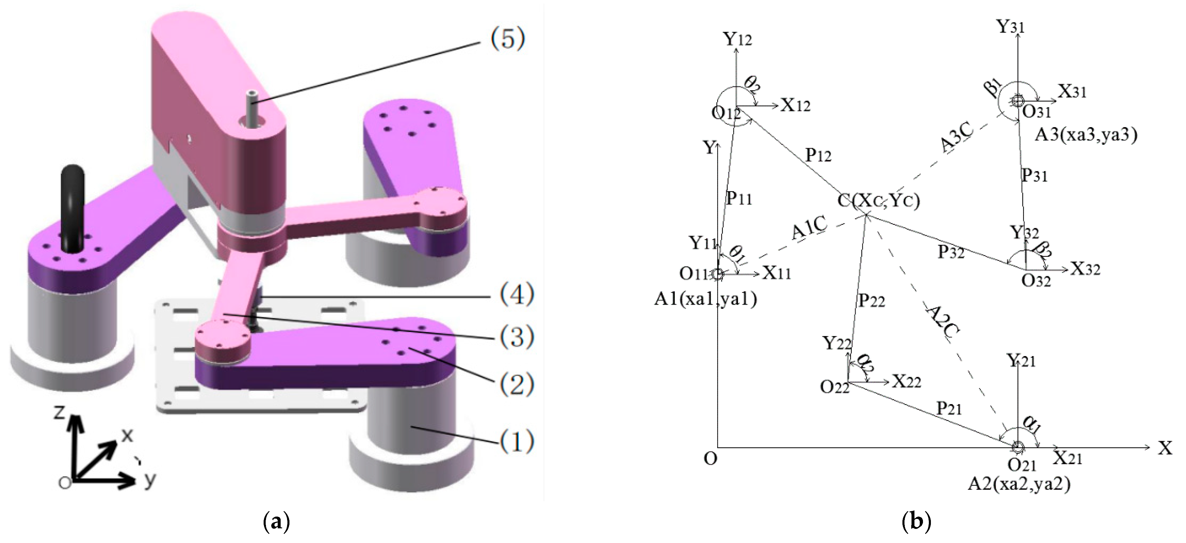
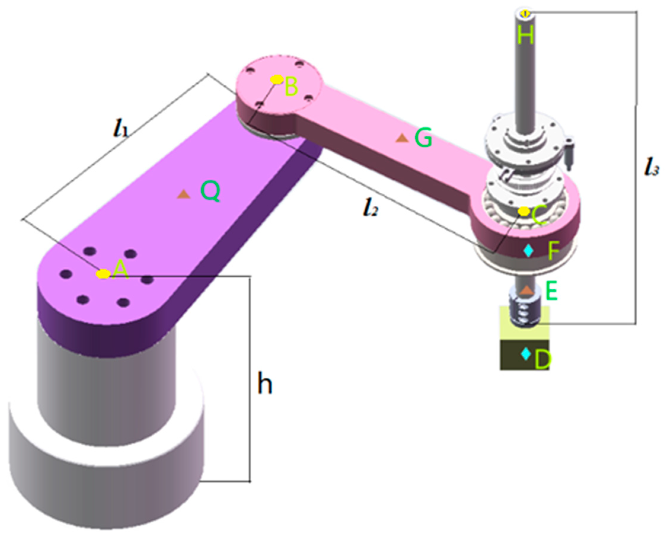
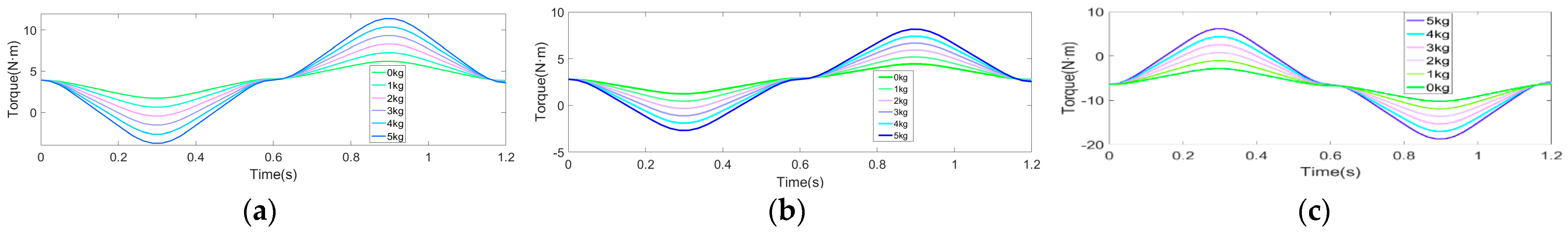
2. Construction of Time-Varying Dynamics Model of 4-DOF Redundant Parallel Robots under Variable Load

Figure 1 shows the structural model of the 4-DOF redundant parallel robot and the coordinate relationship of each joint at any time.

To facilitate the analysis of the forces on each joint, any branched chain in Figure 1a was separated from the redundant mechanism that generated over-constraint, and the separated structure was shown in Figure 2.

As shown in Figure 2, in the process of the robot extracting goods, the change of load will be reflected in its mass and volume, thus leading to the change of the position of the system’s centroid. When applying the Lagrange equation to calculate the torque of each joint, the position and posture of each joint and the coordinate position of the system’s centroid should be determined first. Suppose the three branch chains of the 4-DOF redundant parallel robot subscripts i are 1, 2, and 3, respectively. For a single chain, its base center at point $\mathrm{A}\left({\mathrm{x}}_{{\mathrm{a}}_{\mathrm{i}}},{\mathrm{y}}_{{\mathrm{a}}_{\mathrm{i}}},\mathrm{h}\right)$, driving shaft AB and driven shaft BC joint points for $\mathrm{B}\left({\mathrm{x}}_{{\mathrm{b}}_{\mathrm{i}}},{\mathrm{y}}_{{\mathrm{b}}_{\mathrm{i}}},\mathrm{h}\right)$, driven shaft, BC, and end-effector HE joint points for $\mathrm{C}\left({\mathrm{x}}_{c_{\mathrm{i}}},{\mathrm{y}}_{{\mathrm{c}}_{\mathrm{i}}},\mathrm{h}\right)$. The AB rod length, centroid, centroid distance AQ, and mass are $l_1$, $\mathrm{Q}\left({\mathrm{x}}_{\mathrm{qi}},{\mathrm{y}}_{\mathrm{qi}},{\mathrm{z}}_{\mathrm{qi}}\right)$, ${\mathrm{P}}_{\mathrm{i}1}$, and ${\mathrm{m}}_{\mathrm{i}1}$, respectively. The BC rod length, centroid, centroid distance BG, and mass are $l_2$, $\mathrm{G}\left({\mathrm{x}}_{\mathrm{gi}},{\mathrm{y}}_{\mathrm{gi}},{\mathrm{z}}_{\mathrm{gi}}\right)$, and ${\mathrm{m}}_{\mathrm{i}2}$, respectively. The AB axis and BC axis are in the same plane of xoy. End-effector HE is a member of the yoz plane with rod length $l_3$, centroid $\mathrm{F}\left({\mathrm{x}}_{\mathrm{fi}},{\mathrm{y}}_{\mathrm{fi}},{\mathrm{z}}_{\mathrm{fi}}\right)$, centroid distance HF ${\mathrm{P}}_{\mathrm{F}}$, and mass $\frac{1}{3}{\mathrm{m}}_{\mathrm{F}}$, which can move up and down in the yoz plane. D $\left({\mathrm{x}}_{\mathrm{di}},{\mathrm{y}}_{\mathrm{di}},{\mathrm{z}}_{\mathrm{di}}\right)$ is the load loaded by end-effector HE. Its distance between the load and base plane is ${\mathrm{Z}}_{\mathrm{C}}$, and the mass is $\frac{1}{3}{\mathrm{m}}_{\mathrm{D}}$. $h_x$ is from the base plane to D. The relevant model parameter information can be found in reference Ref. [9].

According to the above assumptions, the Lagrange multiplier is applied to obtain the joint torque of the driving joints, as shown in Equation (1) [10].

$${\displaystyle \mathrm{\tau }}=\frac{d}{dt}\frac{\partial L}{\partial \dot{q}}-\frac{\partial L}{\partial q}+{\mathsf{\Phi }}_q^T\lambda$$

(1)

$L$ is the sum of the system’s kinetic energy and potential energy in Equation (1), where $q_{\left(6\times 1\right)}={\left[{\mathsf{\theta }}_1,{\mathsf{\theta }}_2,{ \mathsf{\alpha }}_1,{ \mathsf{\alpha }}_2,{ \mathsf{\beta }}_1,{ \mathsf{\beta }}_2\right]}^{\mathrm{T}}$ is the vector of the system coordinates, ${\mathrm{\tau }}_{\left(6\times 1\right)}$ is the vector of the corresponding external force/torque, and ${\lambda }_{\left(6\times 1\right)}$ is the vector of the Lagrangian multipliers associated with the constraint Torques ${\mathsf{\Phi }}_q^T\lambda$.

The complete constraint equations [10] are derived by expression (with i = 1, 2, 3) as follows:

$$\left\{\begin{array}{c}f\left(q\right)={\left[f_1^T, f_2^T, f_3^T\right]}^T\\ {\mathsf{\Phi }}_q\dot{q}=0 with {\mathsf{\Phi }}_q\dot{q}=\frac{\partial \mathrm{f}\left(q\right)}{\partial q} \end{array}\right.$$

(2)

where:

$${\mathsf{\Phi }}_q^T={\left[{\mathsf{\Phi }}_{q1}^T,{ \mathsf{\Phi }}_{q2}^T, { \mathsf{\Phi }}_{q3}^T\right]}^T$$

(3)

Assume that the centroid of end-effector HE in Figure 2 is point F and the load centroid is point D. Then the end-effector HE and the load are regarded as a whole and expressed as FD, and the equivalent centroid point of the two is $\mathrm{E}\left(x_{ei}, y_{ei}, z_{ei}\right)$. When the load is a variable, the coordinates of the centroid E $\left(x_{ei}, y_{ei},z_{ei}\right)$ of the end-effector FD are as follows:

$$\left\{\begin{array}{c}{x}_{ei}=x_{ai}+l_1\mathit{cos}(q_{i1})+l_2\mathit{cos}(q_{i2})\\ y_{ei}=y_{ai}+l_1\mathit{sin}(q_{i1})+l_2\mathit{sin}(q_{i2})\\ z_{ei}=h_x+L_{CD2}\end{array}\right.$$

(4)

In this equation, $q_{i1}$ is the driving angular displacement. $q_{i2}$ is the driven angular displacement. The driven angle is not a variable here, but is only for the convenience of representing and calculating the energy and force/moment of each branch chain. The calculation formula of the driven angle is as follows:

$$\left\{\begin{array}{c}{X}_C={\mathrm{x}}_{a1}+l_1\mathit{cos}(q_{11})+l\mathit{cos}(q_{12})={\mathrm{x}}_{a2}+l_1\mathit{cos}(q_{21})+l_2\mathit{cos}(q_{22})\\ ={\mathrm{x}}_{a3}+l_1\mathit{cos}(q_{31})+l_2\mathit{cos}(q_{32})\\ Y_C={\mathrm{y}}_{a1}+l_1\mathit{sin}(q_{11})+l_2\mathit{sin}(q_{12})={\mathrm{y}}_{a2}+l_1\mathit{sin}(q_{21})+l_2\mathit{sin}(q_{22})\\ ={\mathrm{y}}_{a3}+l_1\mathit{sin}(q_{31})+l_2\mathit{sin}(q_{32})\end{array}\right.$$

(5)

The driven angle $q_{i2}$ is expressed as:

$$q_{i2}=\mathit{arccos}(\frac{X_C-\mathrm{xai}-l_1\mathit{cos}{q}_{\mathrm{i}1}}{l_2})$$

(6)

At the end effector, ${\mathrm{L}}_{\mathrm{CD}2}$ is satisfied with the following equation:

$$\left\{\begin{array}{c}{\mathrm{m}}_{\mathrm{F}}{\mathrm{L}}_{\mathrm{CD}1}={\mathrm{m}}_{\mathrm{D}}{\mathrm{L}}_{\mathrm{CD}2}\\ {\mathrm{L}}_{\mathrm{CD}1}+{\mathrm{L}}_{\mathrm{CD}2}=L_3-P_C\end{array}\right.$$

(7)

In this equation, ${\mathrm{L}}_{\mathrm{CD}1}$ and ${\mathrm{L}}_{\mathrm{CD}2}$ are the lengths of EF and DE respectively, and both are variables.

Because the end effector and the load are jointly supported by three branches, the weight of the end effector and the end load is distributed to the three branches. Thus, it can be concluded that the equivalent mass m_FD of the single-chain end-effector HE and the load equivalent volume FD is:

$${\mathrm{m}}_{\mathrm{FD}}=\frac{1}{3} ({\mathrm{m}}_{\mathrm{D}}+{\mathrm{m}}_{\mathrm{F}})$$

(8)

In this equation, ${\mathrm{m}}_{\mathrm{F}}$ and ${\mathrm{m}}_{\mathrm{D}}$ are the mass of the end-effector and load, respectively.

In combination with Equation (1), the Lagrange multiplier of equivalent volume FD is assumed to be L₃, and its calculation equation is as follows:

$$L_3=E_{\mathrm{K}3}-E_{\mathrm{P}3}$$

(9)

In this equation, the potential energy of equivalent volume FD is $E_{\mathrm{P}3}={\mathrm{m}}_{\mathrm{FD}}{\mathrm{gh}}_{\mathrm{x}}$; I kinetic energy $E_{\mathrm{K}3}$ is:

$${\mathrm{E}}_{\mathrm{K}3}=\frac{1}{2}{\mathrm{m}}_{\mathrm{FD}}\left({\dot{x}}_{ei}{}^2+{\dot{y}}_{ei}{}^2+{\dot{z}}_{ei}{}^2\right)$$

(10)

Similarly, the Lagrange multiplier $L_1$ of the AB manipulator is:

$$L_1=E_{\mathrm{K}1}-E_{\mathrm{P}1}$$

(11)

$$E_{\mathrm{K}1}=\frac{1}{2}{\mathrm{m}}_{\mathrm{i}1}\left({\dot{x}}_Q{}^2+{\dot{y}}_Q{}^2+{\dot{z}}_Q{}^2\right)$$

(12)

In this equation, $\dot{x_Q}$, $\dot{y_Q}$, and $\dot{ z_Q}$ can be obtained according to the centroid coordinates of the AB axis, namely:

$$\left\{\begin{array}{c}{x}_Q=x_{a_i}+P_{i1}cos{q}_{i1}\\ y_Q=y_{a_i}+P_{i1}sin{q}_{i1}\\ z_Q=h\end{array}\right.$$

(13)

Similarly, the Lagrange multiplier $L_2$ of the BC manipulator is:

$$L_2=E_{\mathrm{K}2}-E_{\mathrm{P}2}$$

(14)

$$E_{\mathrm{K}2}=\frac{1}{2}{\mathrm{m}}_{\mathrm{i}2}\left({\dot{\mathrm{x}}}_{\mathrm{G}}{}^2+{\dot{\mathrm{y}}}_{\mathrm{G}}{}^2+{\dot{\mathrm{z}}}_{\mathrm{G}}{}^2\right)$$

(15)

The centroid coordinate equation of the BC axis is:

$$\left\{\begin{array}{c}{x}_G=x_{a_i}+l_{1}cos{q}_{i1}+P_{i2}cos{q}_{i2}\\ y_G=y_{a_i}+l_{1}sin{q}_{i1}+P_{i2}sin{q}_{i2}\\ z_G=h\end{array}\right.$$

(16)

To sum up, the Lagrange multiplier L of a single-chain system can be expressed as follows:

$$\mathrm{L}=\frac{1}{2}{\mathrm{m}}_{\mathrm{i}1}\left({\dot{\mathrm{x}}}_{\mathrm{Q}}{}^2+{\dot{\mathrm{y}}}_{\mathrm{Q}}{}^2+{\dot{\mathrm{z}}}_{\mathrm{Q}}{}^2\right)+\frac{1}{2}{\mathrm{m}}_{\mathrm{i}2}\left({\dot{\mathrm{x}}}_{\mathrm{G}}{}^2+{\dot{\mathrm{y}}}_{\mathrm{G}}{}^2+{\dot{\mathrm{z}}}_{\mathrm{G}}{}^2\right)+\frac{1}{2}{\mathrm{m}}_{\mathrm{FD}}\left({\dot{\mathrm{x}}}_{\mathrm{ei}}{}^2+{\dot{\mathrm{y}}}_{\mathrm{ei}}{}^2+{\dot{\mathrm{z}}}_{\mathrm{ei}}{}^2\right)+{\mathrm{m}}_{\mathrm{FD}}{\mathrm{gh}}_{\mathrm{x}}$$

(17)

Combining Equations (1) and (17), the solution of joint torques of every single chain is as follows:

$${\tau }_{\mathrm{di}}=\left(\begin{array}{c}{\tau }_{d1}\\ {\tau }_{d2}\end{array}\right)=\left(\begin{array}{cc}{\mathrm{D}}_{11}& {\mathrm{D}}_{12}\\ {\mathrm{D}}_{21}& {\mathrm{D}}_{22}\end{array}\right)\left(\begin{array}{c}{\ddot{q}}_{\mathrm{i}1}\\ {\ddot{q}}_{\mathrm{i}2}\end{array}\right)+\left(\begin{array}{cc}{\mathrm{E}}_{11}& {\mathrm{E}}_{12}\\ {\mathrm{E}}_{21}& {\mathrm{E}}_{22}\end{array}\right)\left(\begin{array}{c}{\dot{q}}_{\mathrm{i}1}^2\\ {\dot{q}}_{\mathrm{i}2}^2\end{array}\right)+\left(\begin{array}{cc}{\mathrm{F}}_{11}& {\mathrm{F}}_{12}\\ {\mathrm{F}}_{21}& {\mathrm{F}}_{22}\end{array}\right)\left(\begin{array}{c}{\dot{q}}_{\mathrm{i}1}{\dot{q}}_{\mathrm{i}2}\\ {\dot{q}}_{\mathrm{i}2}{\dot{q}}_{\mathrm{i}1}\end{array}\right)+\mathrm{G}\left(q\right)\left(\begin{array}{c}{q}_{\mathrm{i}1}\\ q_{\mathrm{i}2}\end{array}\right)+{\mathsf{\Phi }}_{qi}^T\lambda$$

(18)

In the equation of (18):

$$\begin{gathered} {\mathrm{D}}_{11}={\mathrm{m}}_{\mathrm{i}1}{\mathrm{p}}_{\mathrm{i}1}^2+{\mathrm{m}}_{\mathrm{i}2}{l}_1^2+{\mathrm{m}}_{\mathrm{i}2}{\mathrm{p}}_{\mathrm{i}2}^2+{\mathrm{m}}_{\mathrm{i}2}{l}_1{\mathrm{p}}_{\mathrm{i}2}\mathit{cos}(q_{\mathrm{i}1}-q_{\mathrm{i}2})+{\mathrm{m}}_{\mathrm{FD}}{l}_1^2+{\mathrm{m}}_{\mathrm{FD}}{l}_2^2+{\mathrm{m}}_{\mathrm{FD}}{l}_1{l}_2\mathit{cos}(q_{\mathrm{i}1}-q_{\mathrm{i}2}) \\ {\mathrm{D}}_{12}={\mathrm{m}}_{\mathrm{i}2}{\mathrm{p}}_{\mathrm{i}2}^2+{\mathrm{m}}_{\mathrm{i}2}{l}_1{\mathrm{p}}_{\mathrm{i}2}\mathit{cos}(q_{\mathrm{i}1}-q_{\mathrm{i}2})+{\mathrm{m}}_{\mathrm{FD}}{l}_2^2+{\mathrm{m}}_{\mathrm{FD}}{l}_1{l}_2\mathit{cos}(q_{\mathrm{i}1}-q_{\mathrm{i}2}) \\ {\mathrm{D}}_{21}={\mathrm{m}}_{\mathrm{i}2}{l}_1{l}_2+{\mathrm{m}}_{\mathrm{i}2}{l}_1{\mathrm{p}}_{2\mathrm{i}}\mathit{cos}\left(q_{\mathrm{i}1}-q_{\mathrm{i}2}\right)+{\mathrm{m}}_{\mathrm{FD}}{l}_1{l}_2+{\mathrm{m}}_{\mathrm{FD}}{l}_1{l}_2\mathit{cos}(q_{\mathrm{i}1}-q_{\mathrm{i}2}) \\ {\mathrm{D}}_{22}={\mathrm{m}}_{\mathrm{i}2}{\mathrm{p}}_{\mathrm{i}2}^2 \\ {\mathrm{E}}_{11}={\mathrm{E}}_{22}=0 \\ {\mathrm{E}}_{12}={\mathrm{E}}_{21}={\mathrm{m}}_{\mathrm{i}2}{l}_1{\mathrm{p}}_{\mathrm{i}2}\mathit{sin}(q_{\mathrm{i}1}-q_{\mathrm{i}2})+{\mathrm{m}}_{\mathrm{FD}}{l}_1{l}_2\mathit{sin}(q_{\mathrm{i}1}-q_{\mathrm{i}2}) \\ {\mathrm{F}}_{12}={\mathrm{F}}_{22}=0 \\ {\mathrm{F}}_{11}={\mathrm{F}}_{21}=-{\mathrm{m}}_{\mathrm{i}2}{l}_1{\mathrm{p}}_{\mathrm{i}2}\mathit{sin}(q_{\mathrm{i}1}-q_{\mathrm{i}2})-{\mathrm{m}}_{\mathrm{FD}}{l}_1{l}_2\mathit{sin}(q_{\mathrm{i}1}-q_{\mathrm{i}2}) \end{gathered}$$

Compared with the state without load, ${\mathrm{m}}_{\mathrm{FD}}{l}_1^2$, ${\mathrm{m}}_{\mathrm{FD}}{l}_2^2$, ${\mathrm{m}}_{\mathrm{FD}}{l}_1{l}_2$, ${\mathrm{m}}_{\mathrm{FD}}{l}_1{l}_2\mathit{cos}(q_{\mathrm{i}1}-q_{\mathrm{i}2}),$ and ${\mathrm{m}}_{\mathrm{FD}}{l}_1{l}_2\mathit{sin}(q_{\mathrm{i}1}-q_{\mathrm{i}2})$ all show nonlinear time-varying disturbance characteristics, which can be further sorted out as:

$${\tau }_{\mathrm{di}}={\mathrm{D}}_i^{\prime }q\ddot{q}+{\mathrm{H}}_i^{\prime }\left(q,\dot{q}\right)+{\mathrm{G}}_i^{\prime }\left(q\right)+{\mathsf{\Phi }}_{qi}^T\lambda$$

(19)

In the equation of (19):

$${\mathrm{H}}_i^{\prime }\left(q,\dot{q}\right)=\left(\begin{array}{cc}{\mathrm{E}}_{11}& {\mathrm{E}}_{12}\\ {\mathrm{E}}_{21}& {\mathrm{E}}_{22}\end{array}\right)\left(\begin{array}{c}{\dot{q}}_{\mathrm{i}1}^2\\ {\dot{q}}_{\mathrm{i}2}^2\end{array}\right)+\left(\begin{array}{cc}{\mathrm{F}}_{11}& {\mathrm{F}}_{12}\\ {\mathrm{F}}_{21}& {\mathrm{F}}_{22}\end{array}\right)\left(\begin{array}{c}{\dot{q}}_{\mathrm{i}1}{\dot{q}}_{\mathrm{i}2}\\ {\dot{q}}_{\mathrm{i}2}{\dot{q}}_{\mathrm{i}1}\end{array}\right)$$

In this equation, ${\mathrm{D}}_i^{\prime }$ is the inertial matrix, ${\mathrm{H}}_i^{\prime }$ is the Coriolis and centrifugal matrix, and ${\mathrm{G}}_i^{\prime }$ is the gravity matrix.

$\left(\begin{array}{cc}{\mathrm{E}}_{11}& {\mathrm{E}}_{12}\\ {\mathrm{E}}_{21}& {\mathrm{E}}_{22}\end{array}\right)$ and $\left(\begin{array}{cc}{\mathrm{F}}_{11}& {\mathrm{F}}_{12}\\ {\mathrm{F}}_{21}& {\mathrm{F}}_{22}\end{array}\right)$ are the Positive Definite Symmetric Matrix. The energy corresponding to the inertia matrix under a single branch is discussed separately. For a single branched chain, the second type of Lyapunov is used to determine its stability, E = $\frac{1}{2}{\dot{q}}^{T}D\dot{q}$; thus, the derivative of E is as follows:

$$\dot{E}=\frac{1}{2}{\dot{q}}^T\dot{\mathrm{D}}\dot{q}+{\dot{q}}^{T}D\ddot{q}=-\frac{1}{2}{\dot{q}}^T\dot{q}\left(3{\mathrm{m}}_{\mathrm{i}2}{l}_1{\mathrm{p}}_{\mathrm{i}2}+3{\mathrm{m}}_{\mathrm{FD}}{l}_1{l}_2)\mathit{sin}(q_{\mathrm{i}1}-q_{\mathrm{i}2}\right)({\dot{q}}_{\mathrm{i}1}-q_{\mathrm{i}2}+q_{\mathrm{i}1}-{\dot{q}}_{\mathrm{i}2}))$$

Thus, the result of $\dot{E}<0$ shows this system is stable.

To sum it up, the entire parallel robot system’s dynamic model [11] is as follows:

$${\tau }_{\mathrm{d}}={\mathrm{D}}_{\prime }q\ddot{q}+{\mathrm{H}}_{\prime }\left(q,\dot{q}\right)+{\mathrm{G}}_{\prime }\left(q\right)+{\mathsf{\Phi }}_q^T\lambda$$

(20)

where ${\mathrm{D}}_{\prime }=\mathrm{dig}\left({\mathrm{D}}_1^{\prime },{ \mathrm{D}}_2^{\prime },{ \mathrm{D}}_3^{\prime }\right)$, ${\mathrm{H}}_{\prime }={\left[{\mathrm{H}}_1^{\prime }{}^{\mathrm{T}},{\mathrm{H}}_2^{\prime }{}^{\mathrm{T}},{\mathrm{H}}_3^{\prime }{}^{\mathrm{T}}\right]}^{\mathrm{T}}$, $\tau ={\left[{\tau }_1^T, {\tau }_2^T, {\tau }_3^T\right]}^T$, ${\mathsf{\Phi }}_q^T\lambda ={\left[{\mathsf{\Phi }}_{q1}^T\lambda ,{ \mathsf{\Phi }}_{q2}^T\lambda , { \mathsf{\Phi }}_{q3}^T\lambda \right]}^T$.

To eliminate the assumed Lagrangian multipliers of ideal constraint torque from Equation (1), a matrix $R_{\left(6\times 3\right)}$ is assumed, which determines the null space of the matrix ${\mathsf{\Phi }}_q$(${\mathsf{\Phi }}_{q}R=0$) refer to Refs. [12,13].

$$R^T{\tau }_{\mathrm{d}}=R^T[{\mathrm{D}}^{\prime }q\ddot{q}+ \mathrm{H} \prime \left(q,\dot{q}\right)+ \mathrm{G} \prime \left(q\right)]$$

(21)

${\mathsf{\Phi }}_{qi}$ and $R$ are shown as follows:

$${\mathsf{\Phi }}_{qi}=\left[\begin{array}{c}-l_{i1}{S}_{\theta i}-l_{i2}{S}_{\gamma i}-l_{i2}{S}_{\gamma i}\\ -l_{i1}{C}_{\theta i}+l_{i2}{C}_{\gamma i}-l_{i2}{C}_{\gamma i}\end{array}\right]$$

(22)

$$R=\left[\begin{array}{ccc}\hfill \frac{C_{\gamma 1}}{l_{11}}\hfill & \hfill \frac{S_{\gamma 1}}{l_{11}}\hfill & \hfill \frac{-C_{\gamma 1}}{l_{11}}\hfill \\ \hfill \frac{-l_{11}{C}_{\theta 1}-l_{12}{C}_{\gamma 1}}{l_{11}{l}_{12}}\hfill & \hfill \frac{-l_{11}{S}_{\theta 1}-l_{12}{S}_{\gamma 1}}{l_{11}{l}_{12}}\hfill & \hfill \frac{-l_{11}{C}_{\theta 1}+l_{12}{C}_{\gamma 1}}{l_{11}{l}_{12}}\hfill \\ \hfill \frac{C_{\gamma 2}}{l_{21}}\hfill & \hfill \frac{S_{\gamma 2}}{l_{21}}\hfill & \hfill 0\hfill \\ \hfill \frac{-l_{21}{C}_{\theta 2}-l_{22}{C}_{\gamma 2}}{l_{21}{l}_{22}} \hfill & \hfill \frac{-l_{21}{S}_{\theta 2}-l_{22}{S}_{\gamma 2}}{l_{21}{l}_{22}}\hfill & \hfill 0\hfill \\ \hfill \frac{C_{\gamma 3}}{l_{31}}\hfill & \hfill \frac{S_{\gamma 3}}{l_{31}}\hfill & \hfill 0\hfill \\ \hfill \frac{-l_{31}{C}_{\theta 3}-l_{32}{C}_{\gamma 3}}{l_{31}{l}_{32}} \hfill & \hfill \frac{-l_{31}{S}_{\theta 3}-l_{32}{S}_{\gamma 3}}{l_{31}{l}_{32}}\hfill & \hfill 0\hfill \end{array}\right]$$

(23)

where:

$$\left\{\begin{array}{c}\gamma i=q_{i2}\\ \theta i=q_{i1}\end{array}\right.$$

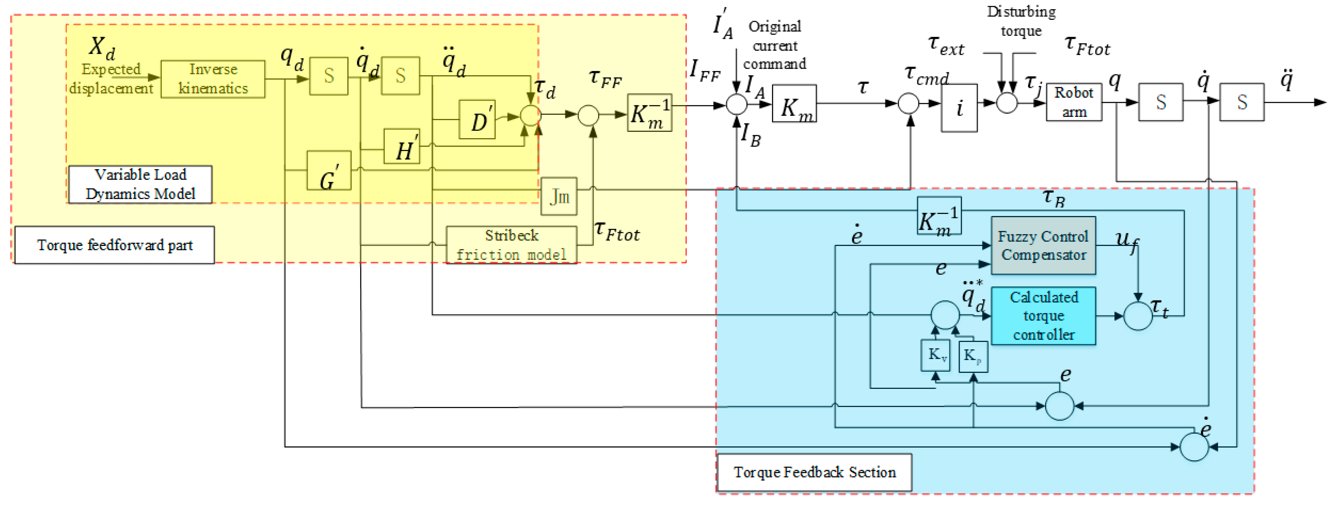
3. Establishment of Hybrid Torque Control Model

Under the condition of variable load, the load has the characteristics of time-varying and nonlinear strong coupling. In this case, the dual-torque feedforward decoupling control method is proposed for the measurable but uncontrollable friction torque and the disturbance torque caused by the operation of the variable load. Meanwhile, as the feedforward control has difficulty resisting other unknown disturbances, the fuzzy computational torque feedback control method is adopted to improve the stability and motion accuracy of the system. The control block diagram of the system after the combination of the two is shown in Figure 3.

3.1. Feedforward Control of Variable Load Disturbance and Friction Torque

The control system based on error feedback has the characteristics of delay and slow response. Therefore, it is particularly important to estimate the load and friction disturbances in advance and decouple the robot joints with torque feedforward. In feedforward control, the end-execution trajectory was mapped to the joint space using inverse kinematics, and the velocity and acceleration expressions of the joint space at any time of the optimized trajectory were obtained under variable load. Based on the dynamic theory of the robot under variable load, the nonlinear time-varying disturbance ${\tau }_d$ of the robot joint under variable load was predicted by the Lagrange operator. The predicted disturbance torque ${\tau }_{d1}$ decoupled the torque loop system by feedforward compensation. The Stribeck friction model and parameter identification technology are used to predict the friction loss torque ${\tau }_f$ of robot joints, and the predicted friction torque is decoupled by feedforward compensation. The structure diagram of the torque feedforward compensation part is shown in Figure 4.

The feedforward torque ${\tau }_{FF}$ is expressed as:

$${\tau }_{FF}={\tau }_{d1}+{\tau }_f$$

(24)

In this equation, the friction torque ${\tau }_f$ is obtained by identification, and the predicted disturbance torque ${\tau }_{d1}$ (for robot arm movement under variable load disturbance) is obtained by Equation (19), which is calculated from the improved dynamics model in Section 2.

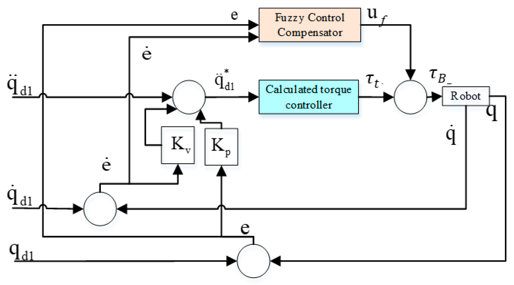
3.2. Calculation and Fuzzy Torque Feedback Control

Feedforward control alone has difficulty resisting other unknown disturbances and the system stability is poor. Therefore, a fuzzy calculation torque feedback control is proposed to compensate for the motion error. The structure diagram of torque feedback control is shown in Figure 5.

$${\tau }_B={\tau }_t+u_f$$

(25)

The output of the calculated torque controller is ${\tau }_t$, the output torque of the fuzzy controller is $u_f$, and the feedback control torque is ${\tau }_i$.

3.2.1. Calculation Torque Controller Design

The torque control method of each branch chain is as follows:

$$\left\{\begin{array}{c}{\tau }_t=\widehat{M}\left(q\right){\ddot{q}}^{\ast }+\widehat{C}{\dot{q}}^2+\widehat{G}\widehat{q}+{\tau }_F\\ {\ddot{q}}^{\ast }={\ddot{q}}_d+K_v\dot{e}+K_{p}e \end{array}\right.$$

(26)

In this equation, $\widehat{M}$, $\widehat{C}$, and $\widehat{G}$ are the inertia matrix, centrifugal and Coriolis matrix, and gravity matrix estimated by Lagrange equation, respectively; ${\ddot{q}}^{\ast }$ is the control variable, and the angular displacement error and angular velocity error are $e$ and $\dot{e}$, respectively, as follows:

$$\left\{\begin{array}{c}e=q_d-q \\ \dot{e}={\dot{q}}_d-\dot{q} \end{array}\right.$$

(27)

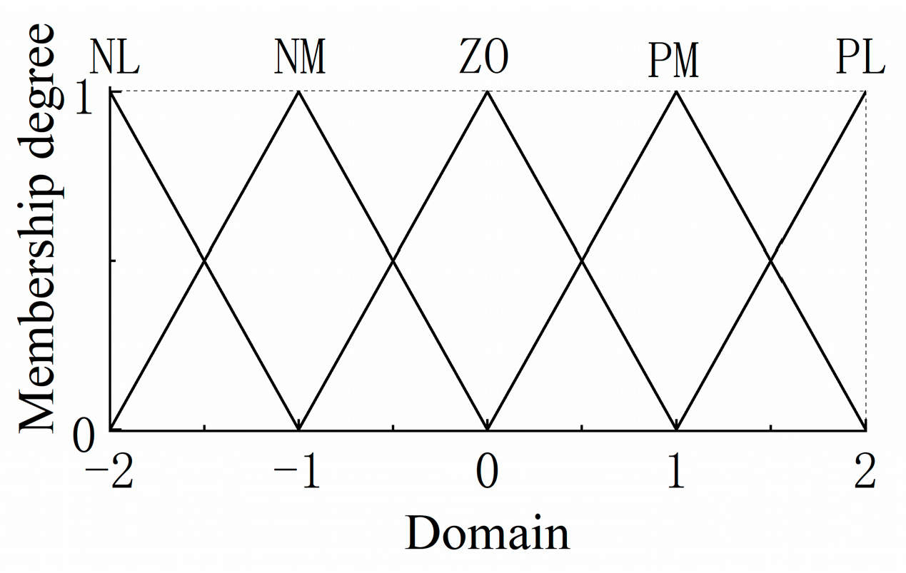
3.2.2. Fuzzy Controller Design

Firstly, the language variables of the fuzzy [14] logic controller are determined. Both the single joint angular displacement deviation $e$ and angular displacement deviation variation rate $\dot{e}$ of the robot are selected as input variables, and the fuzzy logic compensation moment $u_j^{\ast }$ is used as an output variable to design the fuzzy controller [14]. Firstly, the input variable of the robot single joint is defined: angular displacement deviation $e$ and angular displacement deviation variation rate $\dot{e}$ is [−2, −1, 0, 1, 2]. Fuzzy subset definition:

$$\left\{\begin{array}{c}\mathrm{N}\mathrm{B}\left(\mathrm{Negative} \mathrm{Big}\right), \mathrm{N}\mathrm{M}\left(\mathrm{Negative} \mathrm{Middle}\right), \mathrm{Z}\mathrm{O}\left(\mathrm{Zero}\right), \mathrm{P}\mathrm{M}\left(\mathrm{Positive} \mathrm{Middle}\right), \mathrm{P}\mathrm{B}\left(\mathrm{Positive} \mathrm{Big}\right) \end{array}\right\}$$

Secondly, the membership function is determined as shown in Figure 6, and fuzzy rules are established as shown in

Table 1. Fuzzy rules table.

	$u_f$	$\dot{e}$
$e$		NB	NM	ZO	PM	PB
NB		NB	NB	NB	NM	NM
NM		NM	NM	NM	NM	PM
ZO		NB	NM	PM	PM	PB
PM		NM	PM	PM	PM	PB
PB		PM	PM	PB	PB	PB

.

Finally, fuzzy logic reasoning and defuzzification are used. In MATLAB, the fuzzy control toolbox is used to write input and output membership functions and fuzzy control rule table. According to the regular control statement, the Mamdani method is used to deduce the corresponding relationship between the angular displacement deviation, angular displacement deviation variation rate, and the output $u_f$. Finally, the center of gravity method is used to denazify the output, so that the output $u_f$ can partially compensate for the torque.

Using the second Lyapunov theory analysis, the stability of calculating torque control, the analysis process is as follows:

$$\begin{array}{c}{\tau }_t=M\left(q\right)\ddot{q}+C\left(q,\dot{q}\right)+G\left(q\right)=K_{p}e-K_v\dot{q}+\end{array}G\left(q\right)$$

$$M\left(q\right)\ddot{q}+C\left(q,\dot{q}\right)+K_v\dot{q}+K_{p}q=K_p{q}_d$$

(28)

Its energy equation:$\mathrm{E}=\frac{1}{2}{\dot{q}}^{T}M\left(q\right)\dot{q}+\frac{1}{2}{\mathrm{e}}^T{K}_p\mathrm{e}$, where the $M$ and $K_p$ are greater than zero.

Then, the derivative of the energy equation is:

$$\dot{E}={\dot{q}}^{T}M\left(q\right)\ddot{q}+\frac{1}{2}{\dot{q}}^T\dot{M}\left(q\right)\dot{q}-{\mathrm{e}}^T{K}_p\dot{q}=\frac{1}{2}{\dot{q}}^T\dot{M}\left(q\right)\dot{q}-{\dot{q}}^T{K}_v\dot{q}+\dot{q}C\left(q,\dot{q}\right)=-{\dot{q}}^T{K}_v\dot{q}$$

(29)

Because the $K_v$ is always positive, and the $\dot{E}$ is always non-positive, the system is stable.

4. Simulation and Experiment

4.1. Simulation Results

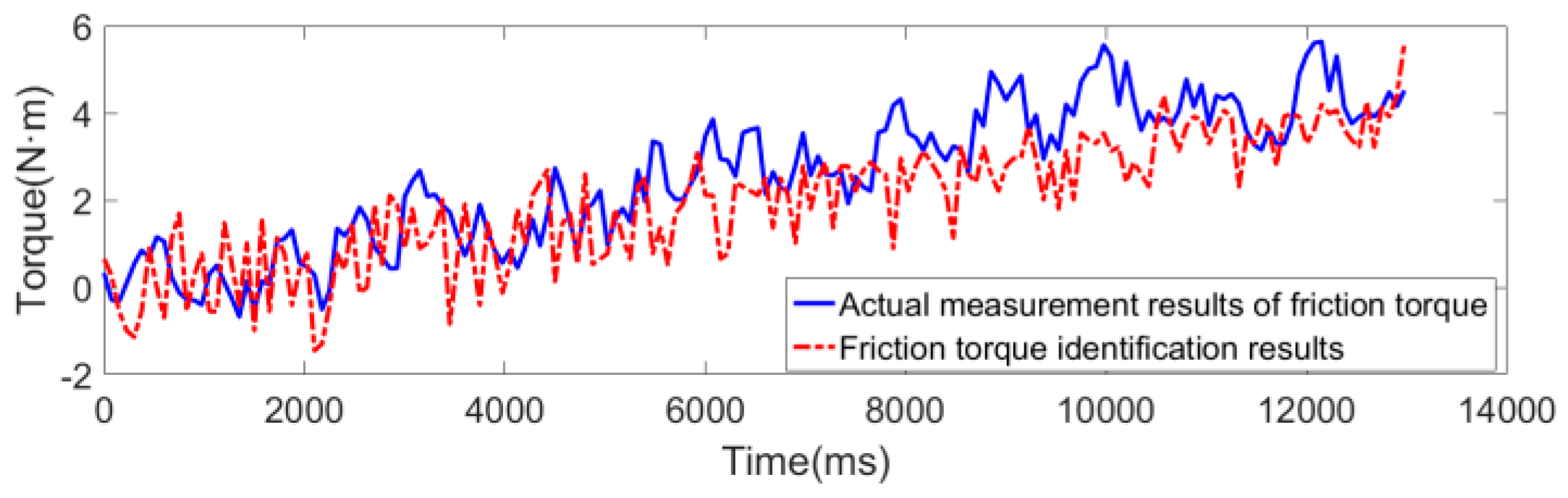
Parameter Identification Results of Stribeck Friction Model

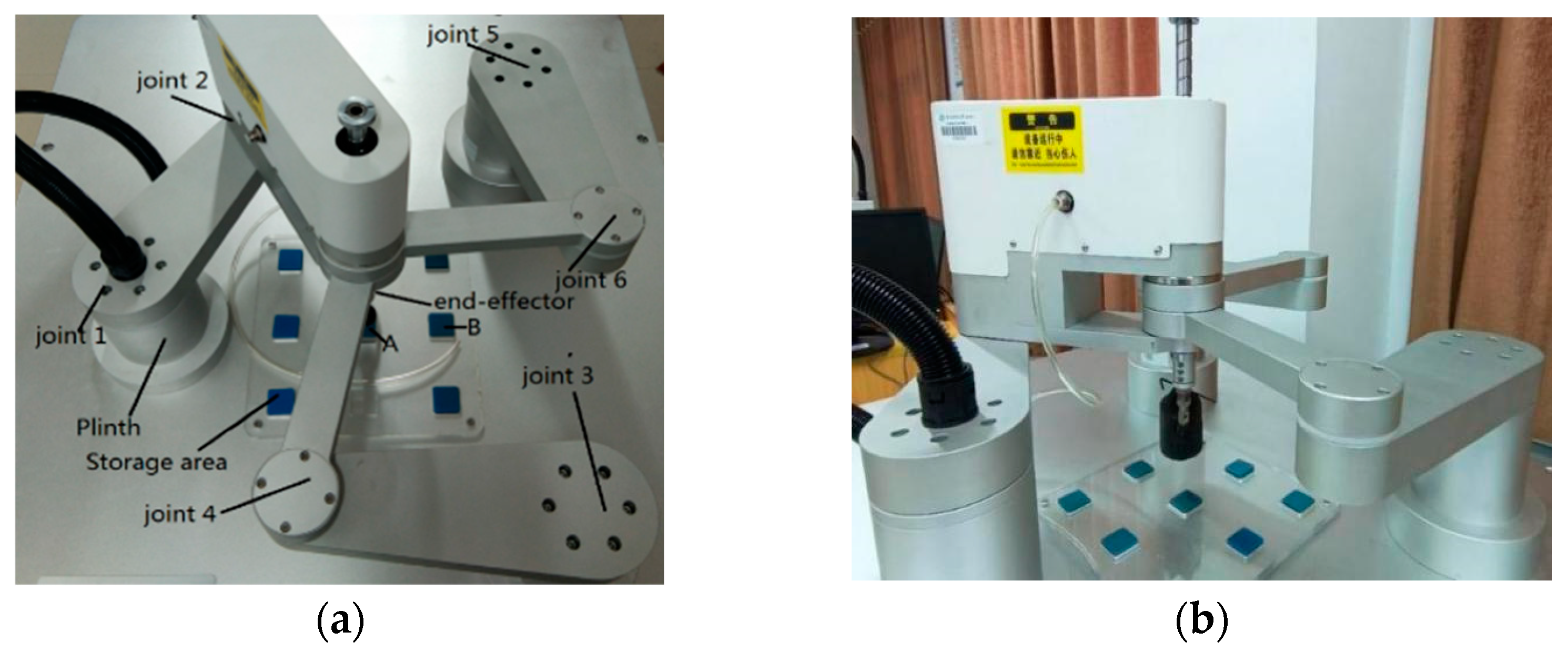
The parameter identification process of the basic Stribeck friction model is based on multiple off-line measurements of the robot’s single joint at different constant velocities (when the robot moves at constant velocities, the inertia matrix, centrifugal, and Coriolis moment are zero; because when the 4-DOF redundant robot moves in xoy plane, the heavy torque is zero, namely: $\tau ={\tau }_{Ftot}$), the relationship between friction torque and rotational speed can be obtained referring to Refs. [15,16,17,18,19,20,21]. The Stribeck friction model function of the joint is shown as:

$${\tau }_f=f_{Fv}\omega +[{\tau }_{Fc}+\left({\tau }_{\mathrm{s}}-{\tau }_{Fc}\right)e^{\left(-\frac{\mathsf{\omega }}{{\mathsf{\omega }}_s}\right)\delta }]sgn\left(\mathsf{\omega }\right)$$

(30)

The four parameters to be identified were calculated at four points. Finally, the L-M (Levenberg-Marquardt) algorithm was used to fit the model. The final parameter identification results are shown in

Table 2. Parameter identification results of the Stribeck model.

${\tau }_{Fc}$	${\tau }_{Fs}$	${\omega }_s$	$f_{Fv}$
0.11	0.14	11.077	4.0216 × 10−4

:

Converting the joint friction torque to the torque-producing motor needs to be multiplied by the reduction ratio, so the comparison between the measured friction torque and parameter identification results of the robot in normal operation is shown in Figure 7.

It can be seen from Figure 8 that the parameter identification result of the friction torque is close to the actual measured value, which is evaluated by the goodness of fit $R^2$ evaluation model in Ref. [15]. The goodness of fit is 0.9355, close to 1, which is good. Therefore, the parameter identification result of this model is relatively reliable.

According to the friction torque ${\tau }_f,$ and the calculation and identification of the torque ${\tau }_d$ of the robot arm under the disturbance of the variable load in the dynamic model calculation of the variable load in 2.1, the simulation results of the feedforward compensation torque of the driving joint under different loads are shown in Figure 8.

4.2. Experiment

4.2.1. Experimental Design

The GPM-II 4-DOF redundant parallel robot was connected to the control PC through a serial port, the motion mode was changed to torque mode in the driver debugging software “Servo Studio”, and the forward and inverse dynamics module under variable loads were established under the Gtrbox toolbox developed in MATLAB.

In “Torque Mode”, a Control strategy combining feedforward and feedback with friction torque and variable load dynamics model is used to control the joint torque of a 4-DOF redundant parallel robot in “Control”.

In the feedforward experiment of a 4-DOF redundant parallel robot under variable load, the loading weight is determined to be in the range of 0–5 kg, according to the rated load capacity of the driving motor. Therefore, loads of 0 kg, 1 kg, 2 kg, 3 kg, 4 kg, and 5 kg were applied to the end-effector, respectively. The field equipment and experimental figure are shown in Figure 9.

The single driving joint is operated according to the planned trajectory, and the trajectory tracking experiment is performed in Torque Mode based on the calculated torque and fuzzy control combined with feedback Refs. [11,22,23,24,25,26,27], supplemented by variable load disturbance and friction torque feedforward. The encoder was used to collect the angular displacement variation data under various load conditions, and the angular velocity, angular acceleration, and angular acceleration change rate were obtained through differential and filtering processing. According to the current data recorded by the driving software, the real-time situation of the joint torques in motion under various loads was calculated.

The trajectory in the operating space is the linear motion from A to B. In the joint space, the 12-phase sinusoidal shock curve is used as the motion trajectory; refer to Ref. [9]. The structure and dynamic parameters of the robot are shown in

Table 3. The structure and dynamic parameters of the 4-DOF parallel robot.

Parameter	Quality (Kg)	Length (m)	Distance from Center of Mass to Joint (m)	Moment of Inertia Kg × m2
1	2.1	0.2440	0.1096	0.0252
2	8.5	0.2440	0.0957	0.0778
3	2.1	0.2440	0.1096	0.0252
4	0.4	0.2440	0.1260	0.0064
5	2.1	0.2440	0.1096	0.0252
6	0.4	0.2440	0.1260	0.0064

.

4.2.2. Experimental Results and Analysis

For robot joints within 0–5 kg, the load and the stability of the angular displacement and angular velocity remain the same, and the response speed of the torque control and control stability are improved, respectively, through the simple torque feedback and torque feedback and feedforward to control the robot joints, by comparison with the experimental running characteristics of two kinds of control mode (trajectory tracking error, response time, velocity stability, and control moment), showing the advantages of the combined model of variable load disturbance and friction torque feedforward and fuzzy computational torque feedback control in the aspects of motion accuracy, operation stability, response speed, and control stability.

(A)

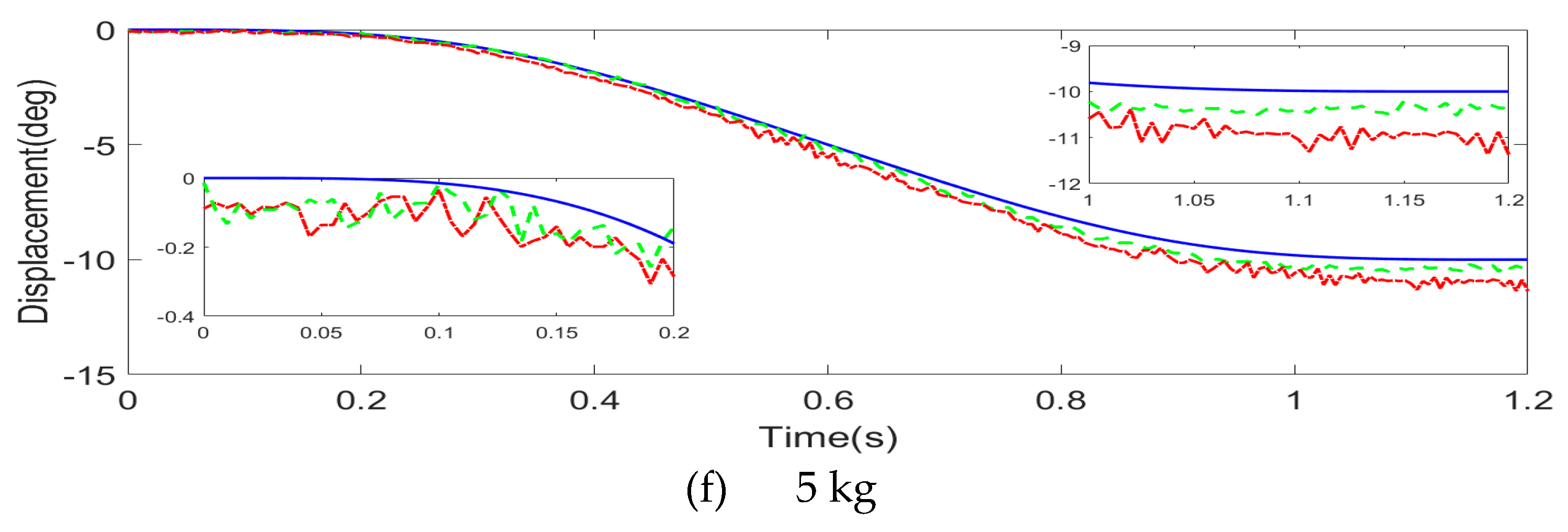
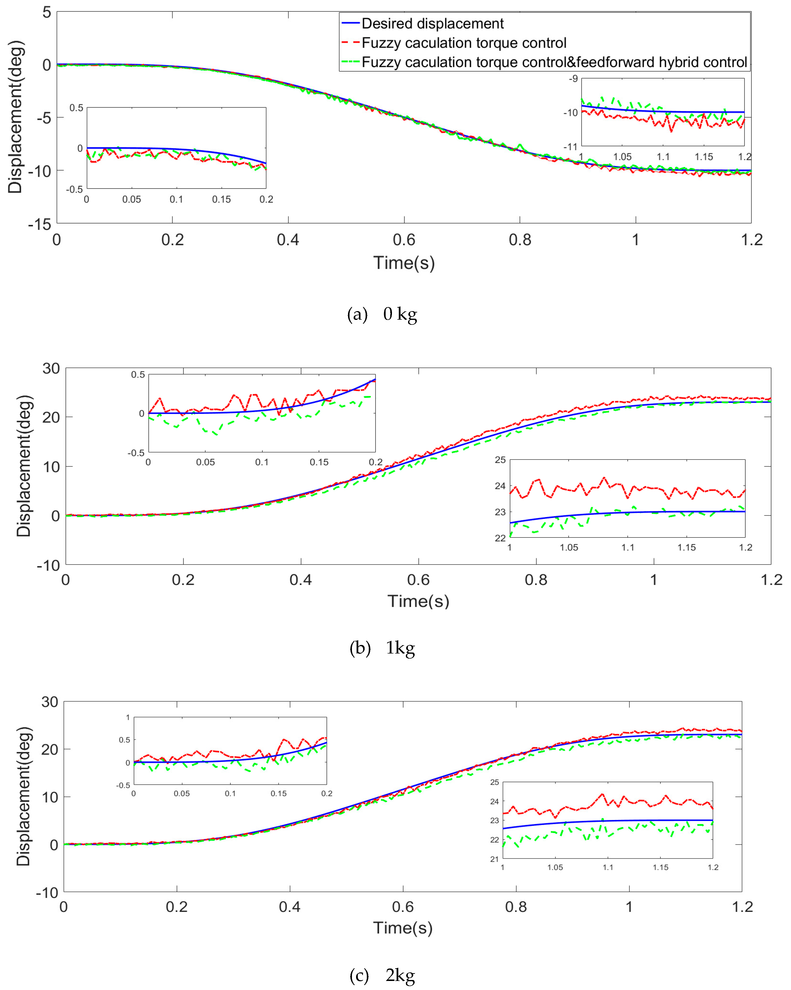
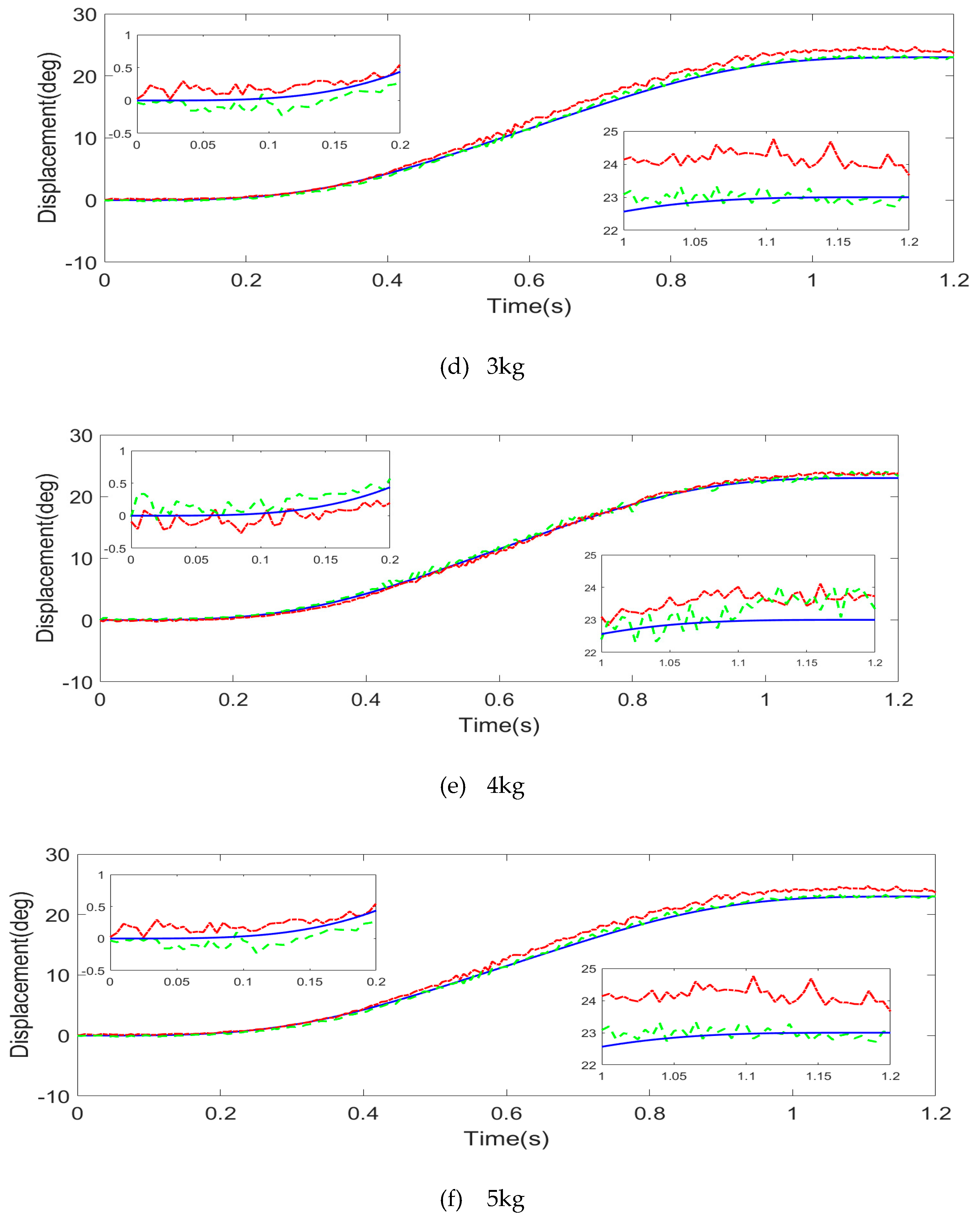
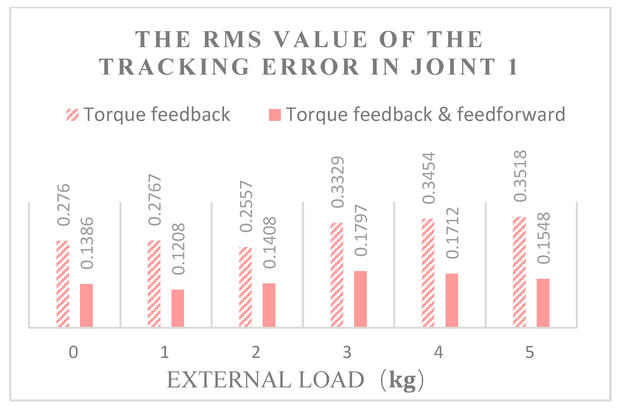
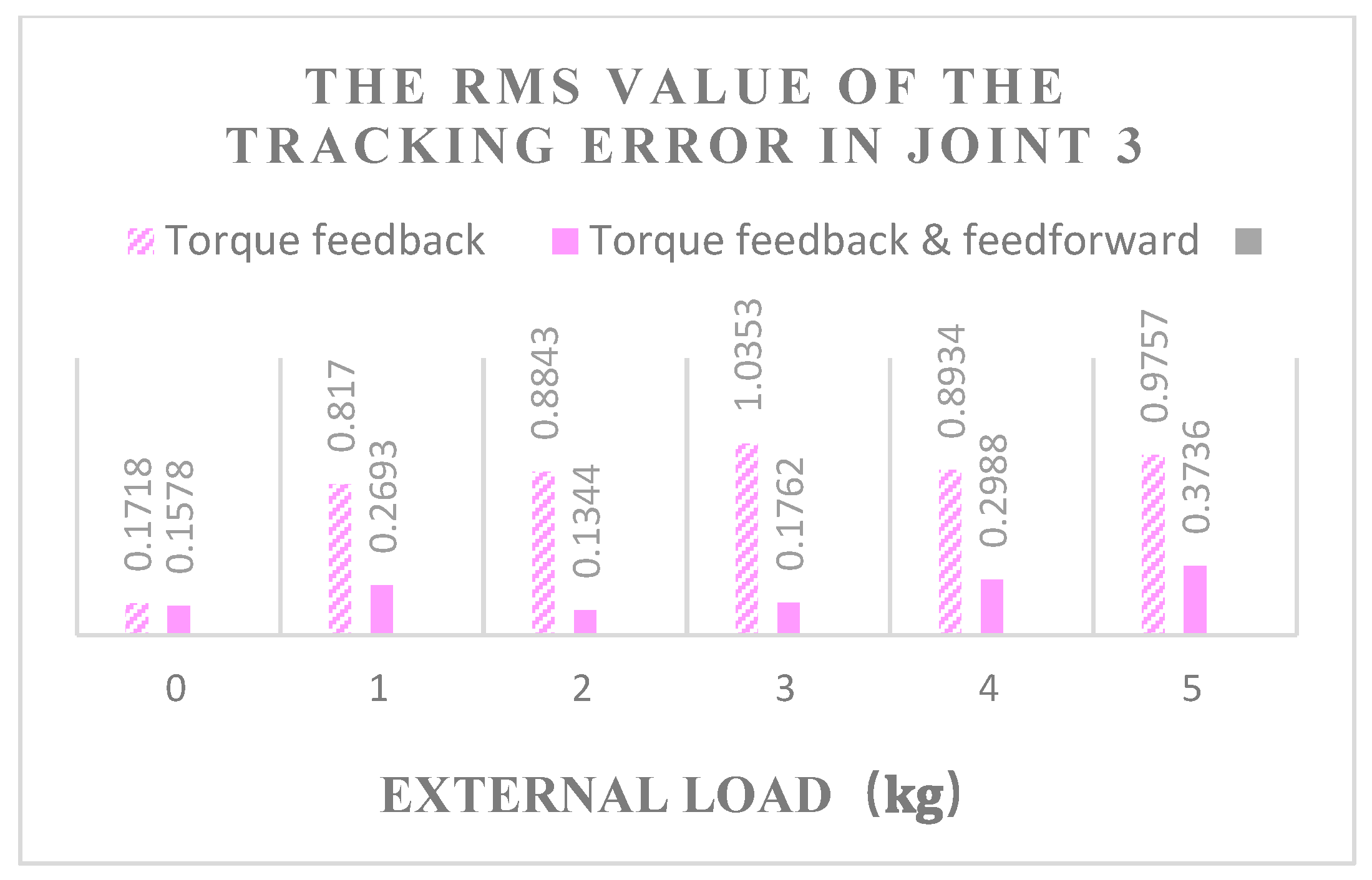
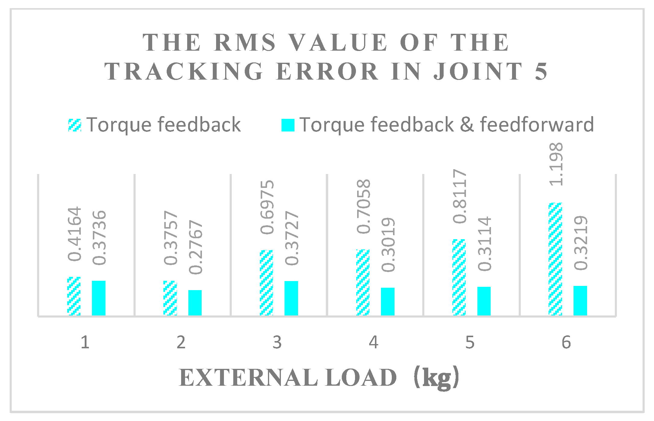
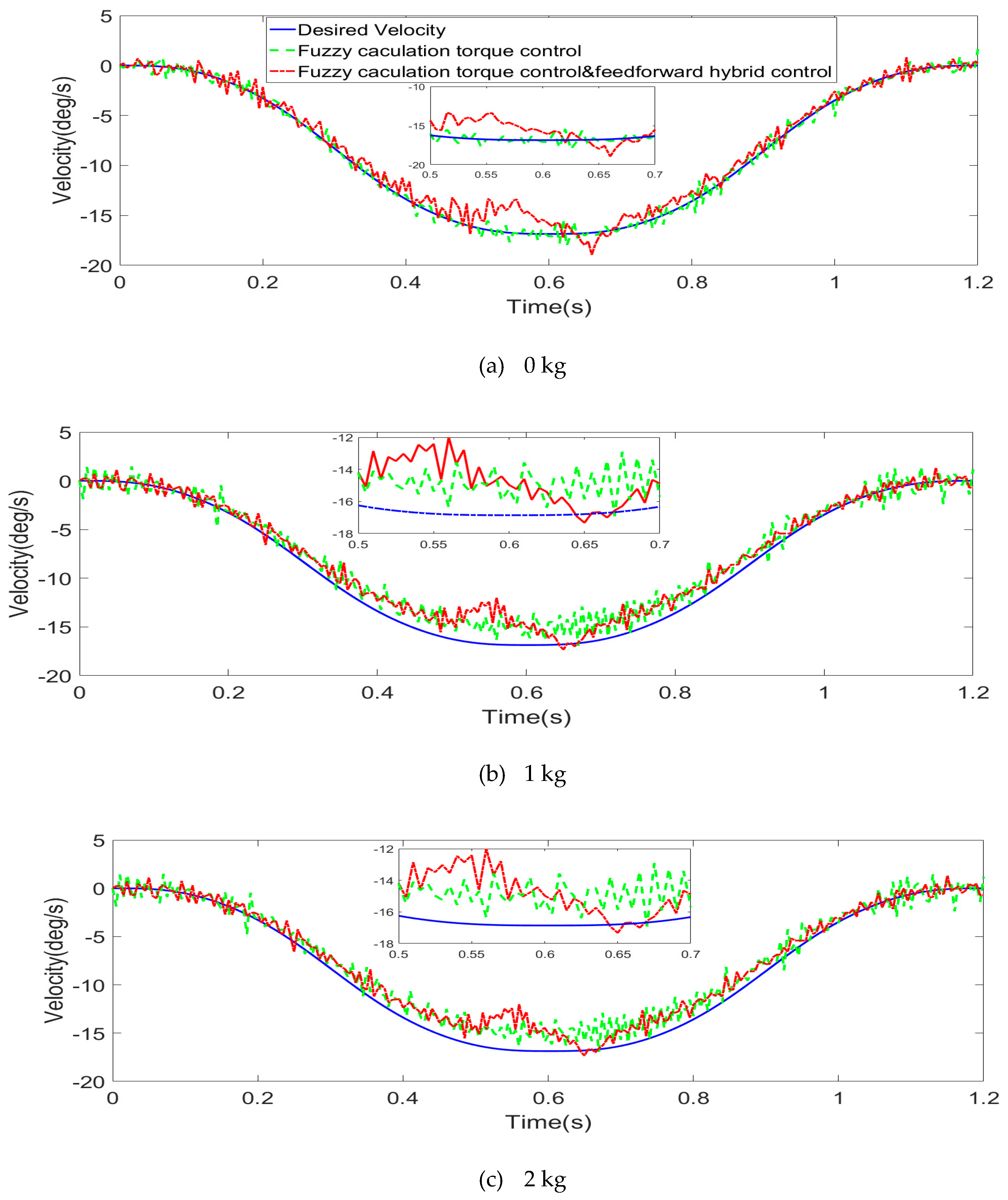
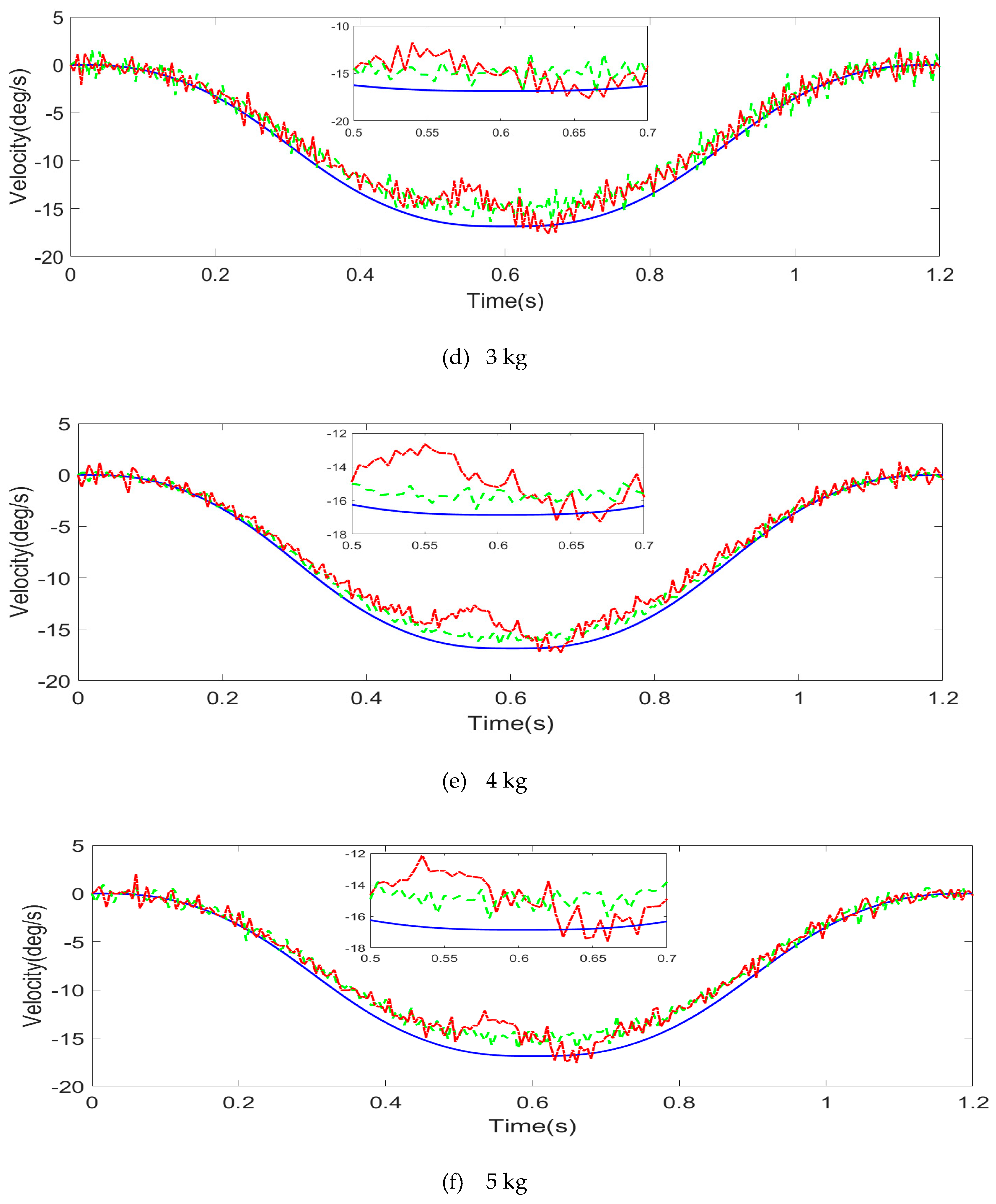
Trajectory tracking error comparison

The feedback control and feedback amp are obtained through experiments under different external loads. Figure 10 shows the comparison of angular displacement under feedforward compensation control.

By Figure 10, Figure 11 and Figure 12, at different loads within 0–5 kg, three driving joints of 4-DOF parallel robotic angular displacements of the experiment are close to the planned trajectory, both in fuzzy computing torque feedback control, and fuzzy calculation and feedforward torque hybrid control. Two kinds of control modes of the angular displacement track are bigger than the planned value because of the influence of accumulated error, and the deviation increases with the increase in movement time. Additionally, the overall motion deviation of the robot under the hybrid torque control is less than that of the fuzzy computational torque feedback control.

The specific numerical analysis of RMS error is shown in Figure 13, Figure 14 and Figure 15.

It can be seen from Figure 13, Figure 14 and Figure 15 that joints 1, 3, and 5 are under different loads of 0–5 kg. As the load increases, the RMS value of the displacement error increases in the fluctuation, and all of their tracking error RMS values in the feedback and feedforward torque hybrid control are less than in one without feedforward control. When the external load is 0, the RMS value of the tracking error of the torque hybrid control is slightly lower than that of the torque feedback. Through calculation, the root values of the trajectory tracking error of feedback and feedforward torque hybrid control in three driving joints are 49.87%, 70.48%, and 50.37% lower, respectively, than that of torque feedback on average; thus, it is concluded that the motion accuracy under torque feedback and feedforward hybrid torque control is higher than that of pure torque feedback control.

(B)

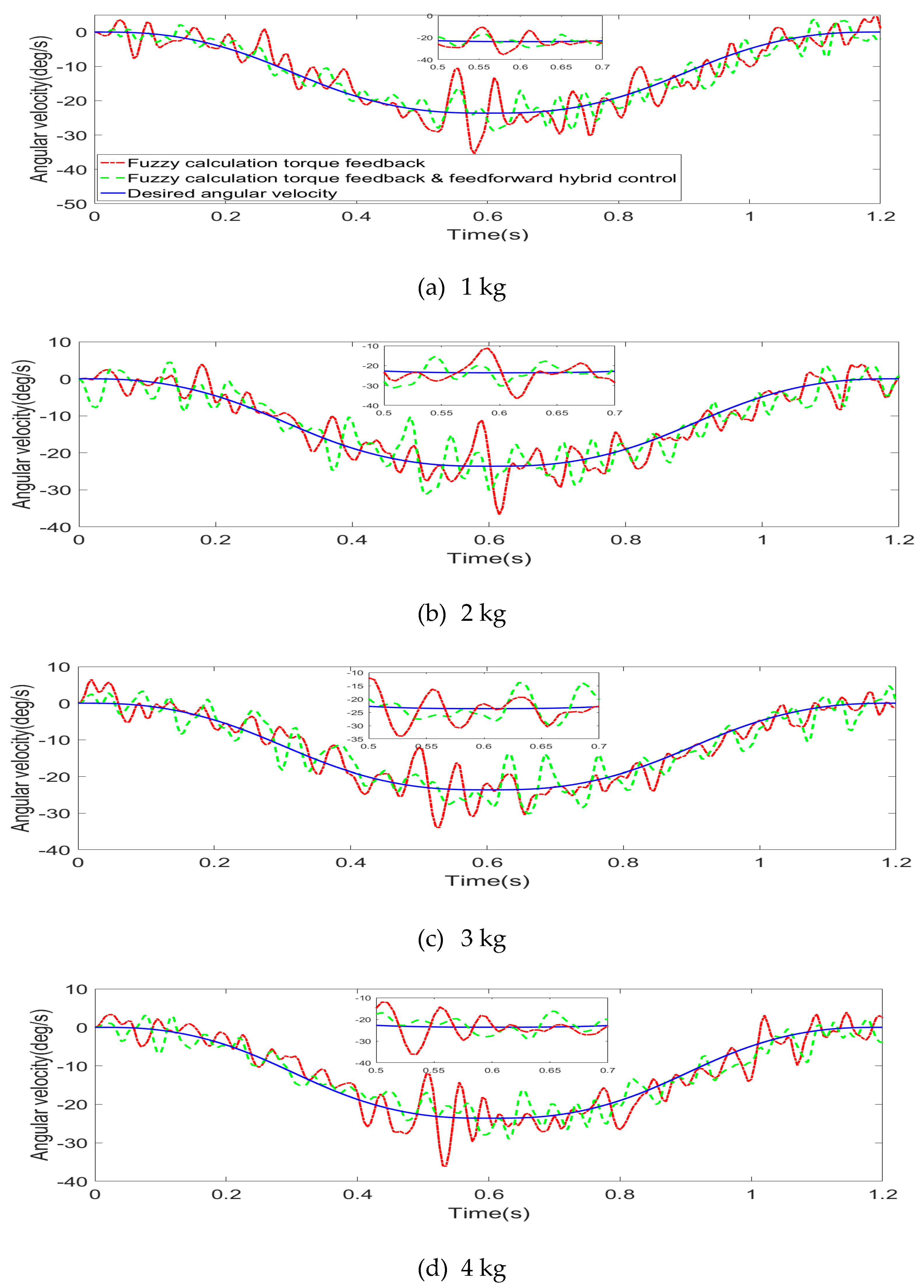
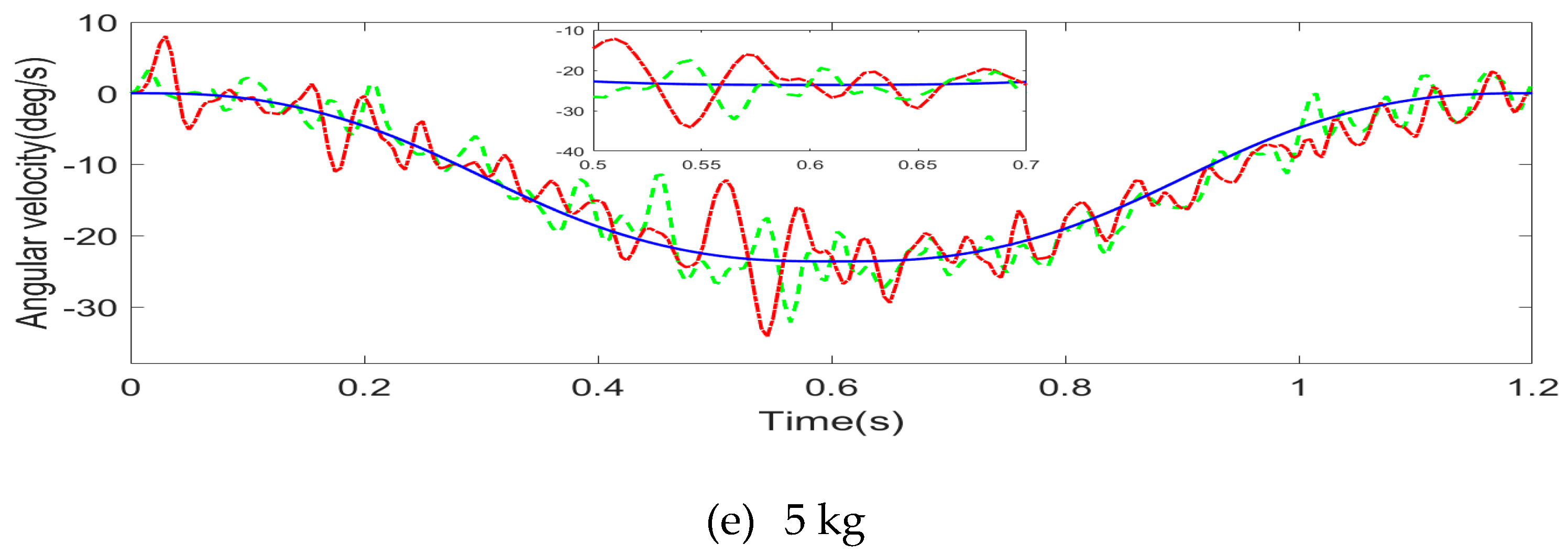
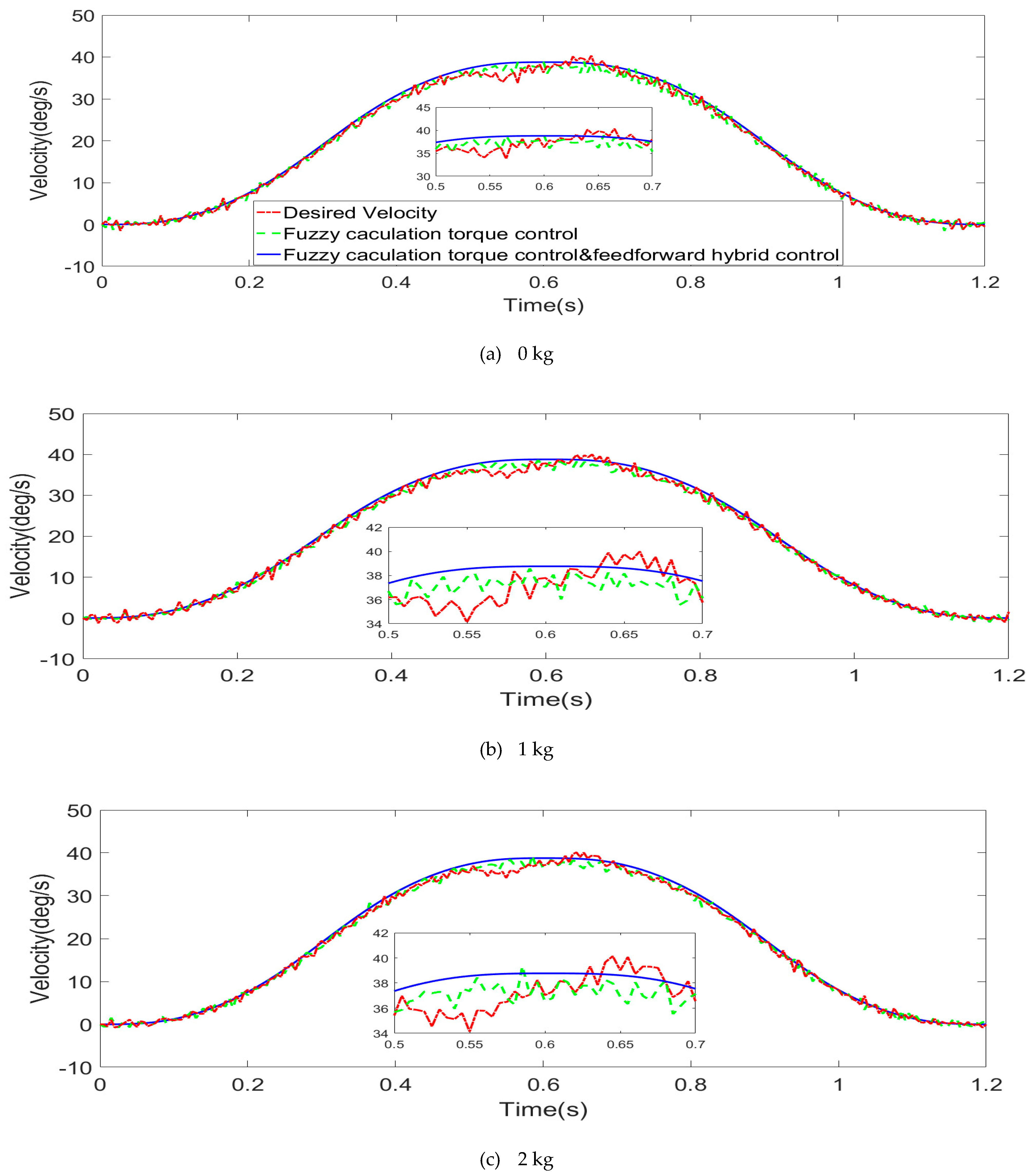
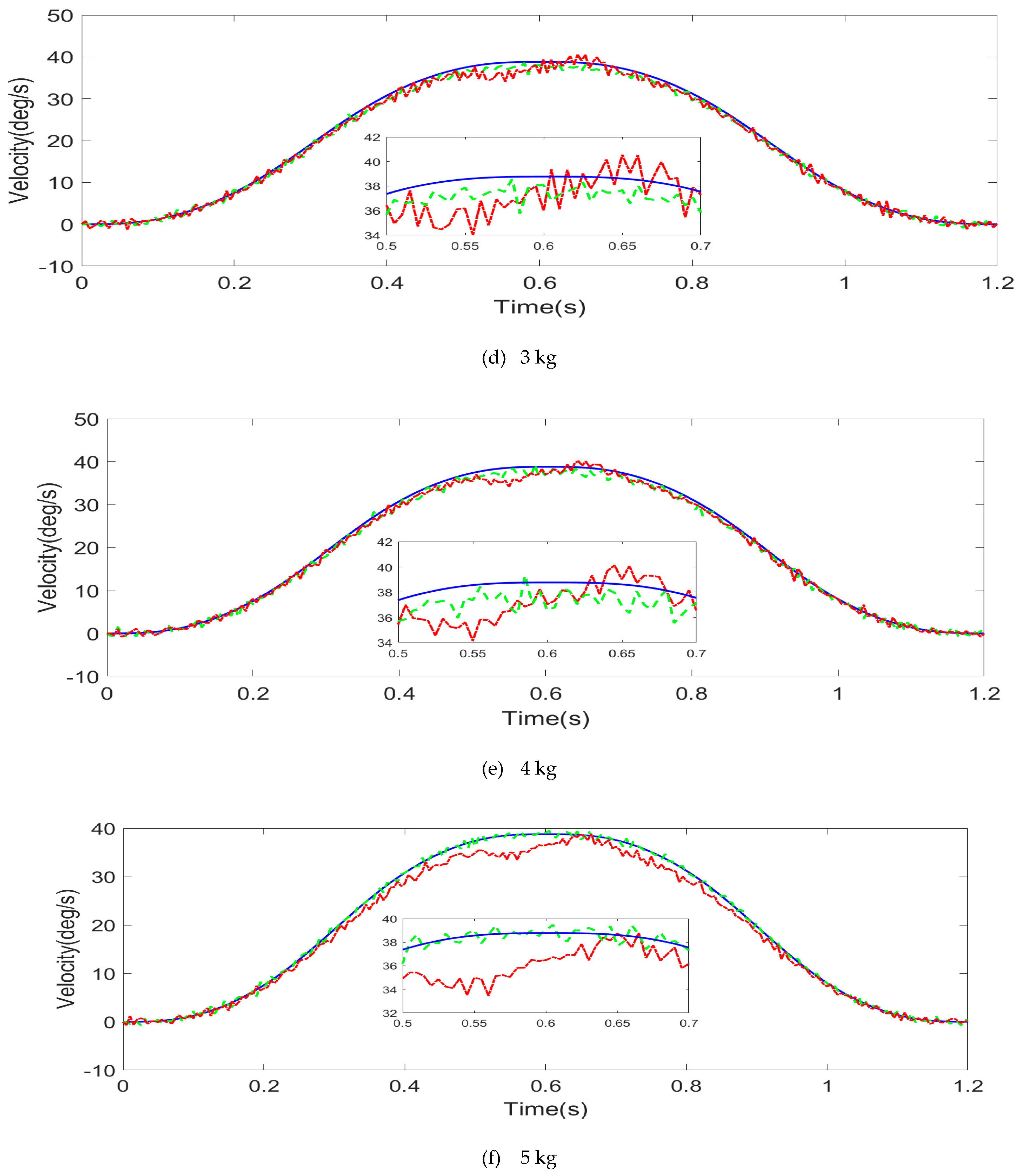
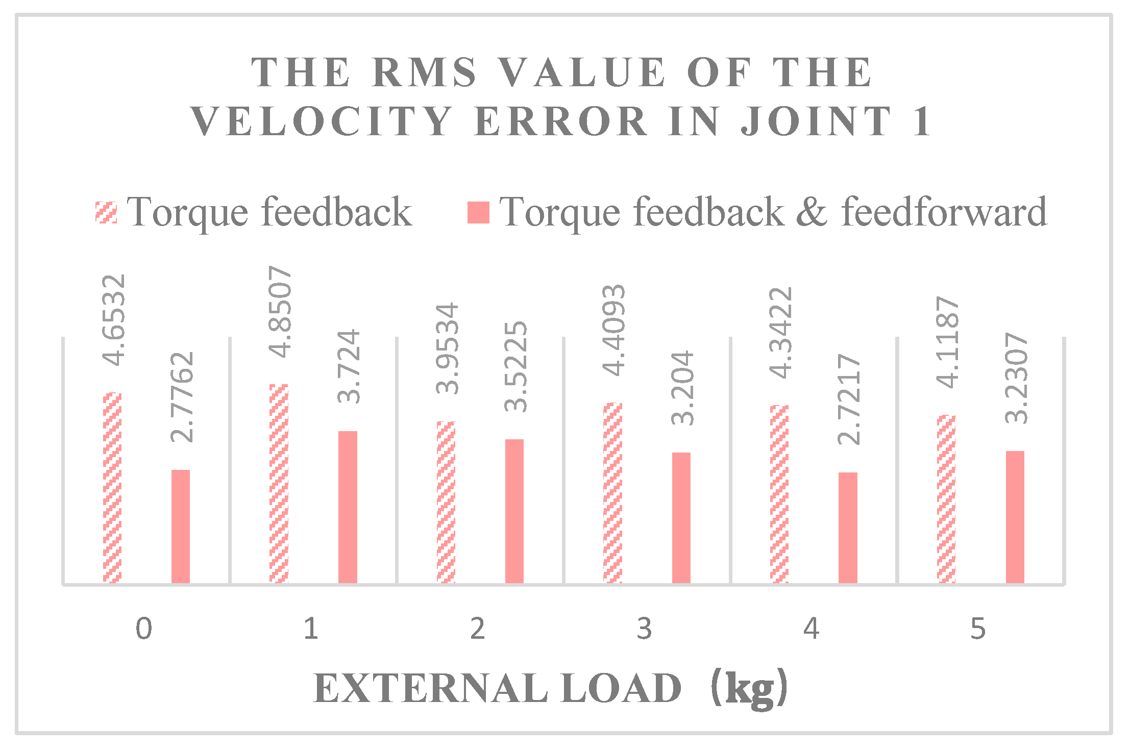
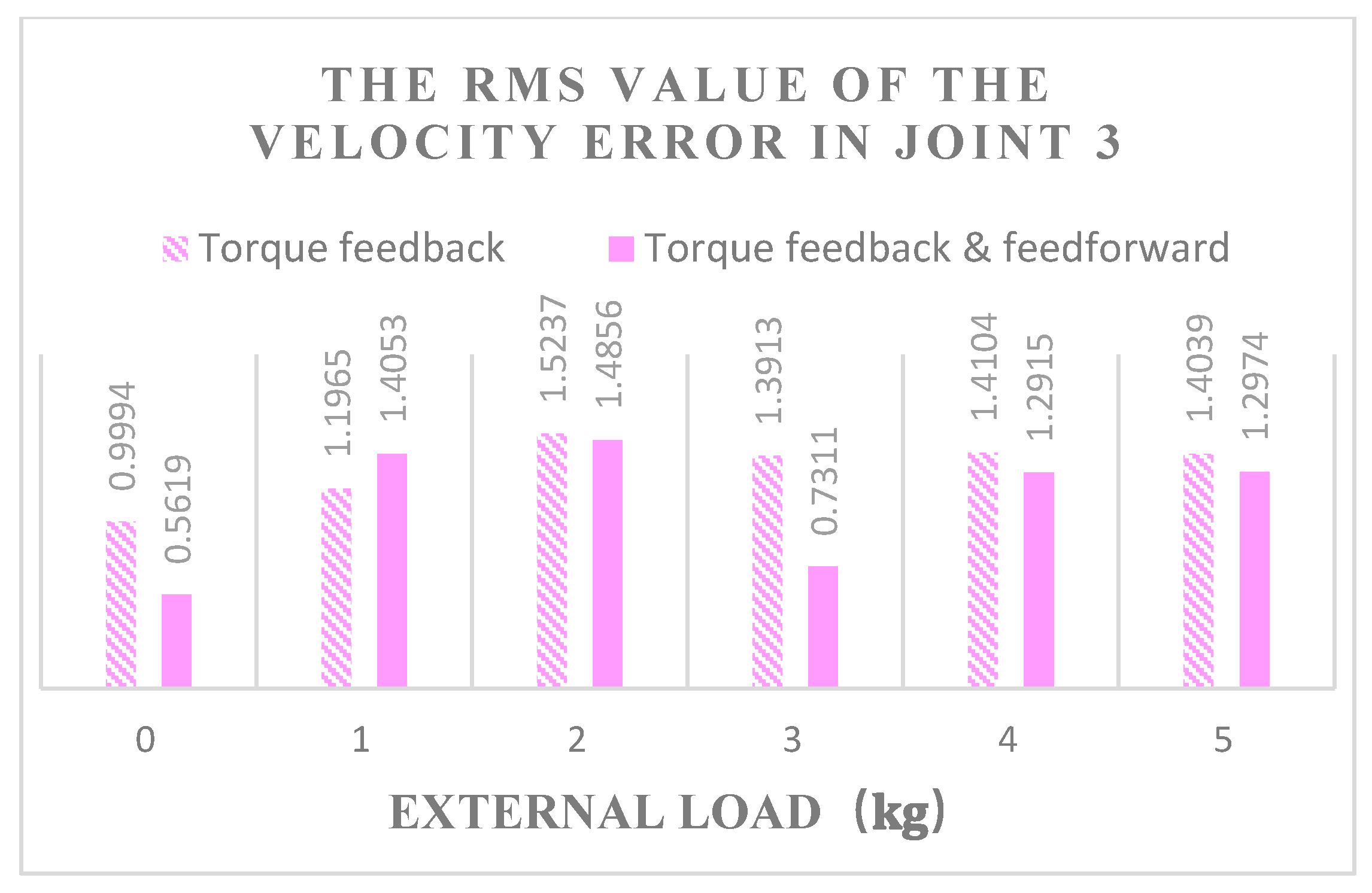
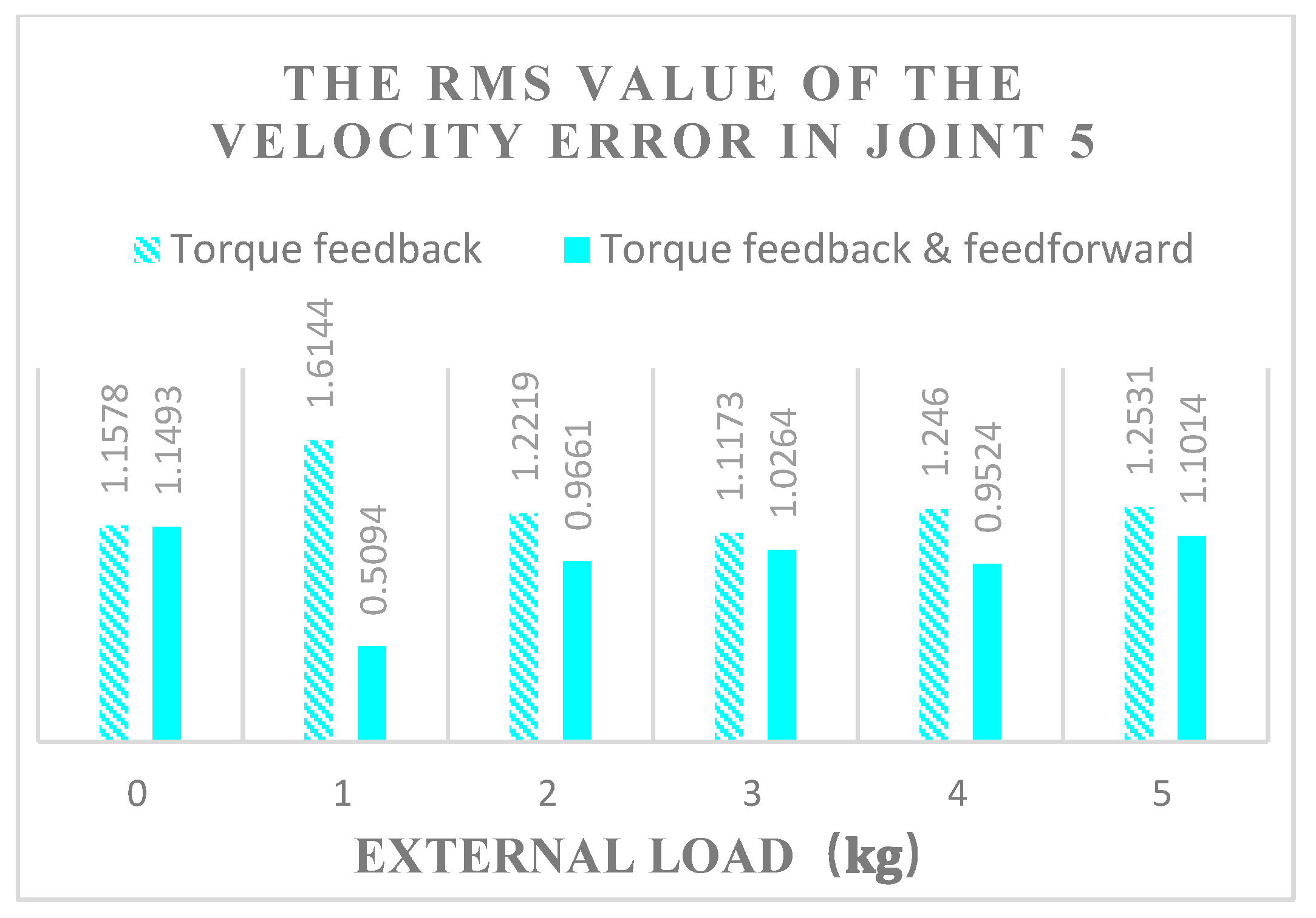
Comparison of velocity stability

By differentiating angular displacement and filtering, feedback control and feedback and feedforward hybrid control are obtained under 0–5 kg load and different external loads. Figure 16, Figure 17 and Figure 18 show the comparison of the angular velocity under feedforward compensation control.

According to Figure 16, Figure 17 and Figure 18, the velocities of the robot joints under the two torque control methods in different loads of 0–5 kg fluctuate around the planned velocities, and both of them are close to the expected velocities. However, the velocity deviations under the feedback and feedforward hybrid torque control are lower than those under the single torque feedback control. The analysis of the velocity stability of the robot joint analyzes the RMS error value between the motion speed and the expected speed. By Figure 13, Figure 14 and Figure 15, the internal angular velocity fluctuation of 0–5 kg load in the feedback and feedforward hybrid toque compensation control is compared with torque feedback control, and its velocity stability is obtained through analysis and calculation, as shown in Figure 19, Figure 20 and Figure 21, respectively.

It can be seen from Figure 19, Figure 20 and Figure 21 that when there is no load, the RMS values of the velocity error of joints 1, 3, and 5 in the torque hybrid control are slightly lower than those of the torque feedback. With the increase in load, the RMS value of velocity error increases in fluctuation, and the overall trend is upward. Through calculation, the average RMS values of the three driving joints’ speed error under torque feedback control are 4.3879, 1.3709, and 1.2684, respectively; the average RMS values of speed error under torque feedback and feedforward control are 3.3632, 1.1288, and 0.9508, respectively; and the speed stabilities of torque hybrid control are relatively higher by 23.35%, 17.66%, and 25.04%, respectively.

5. Conclusions

Based on the modified dynamic model and the Stribeck friction model of joints for a 4-DOF redundant parallel robot under variable loads, this study used the torque feedforward for compensation control and combined the fuzzy computational torque feedback for hybrid control. Through relevant simulation and experiment, a comparison of the key characteristic parameters between fuzzy computational torque feedback and fuzzy computational torque feedback & torque feedforward hybrid control was performed. The conclusions of this study are as follows:

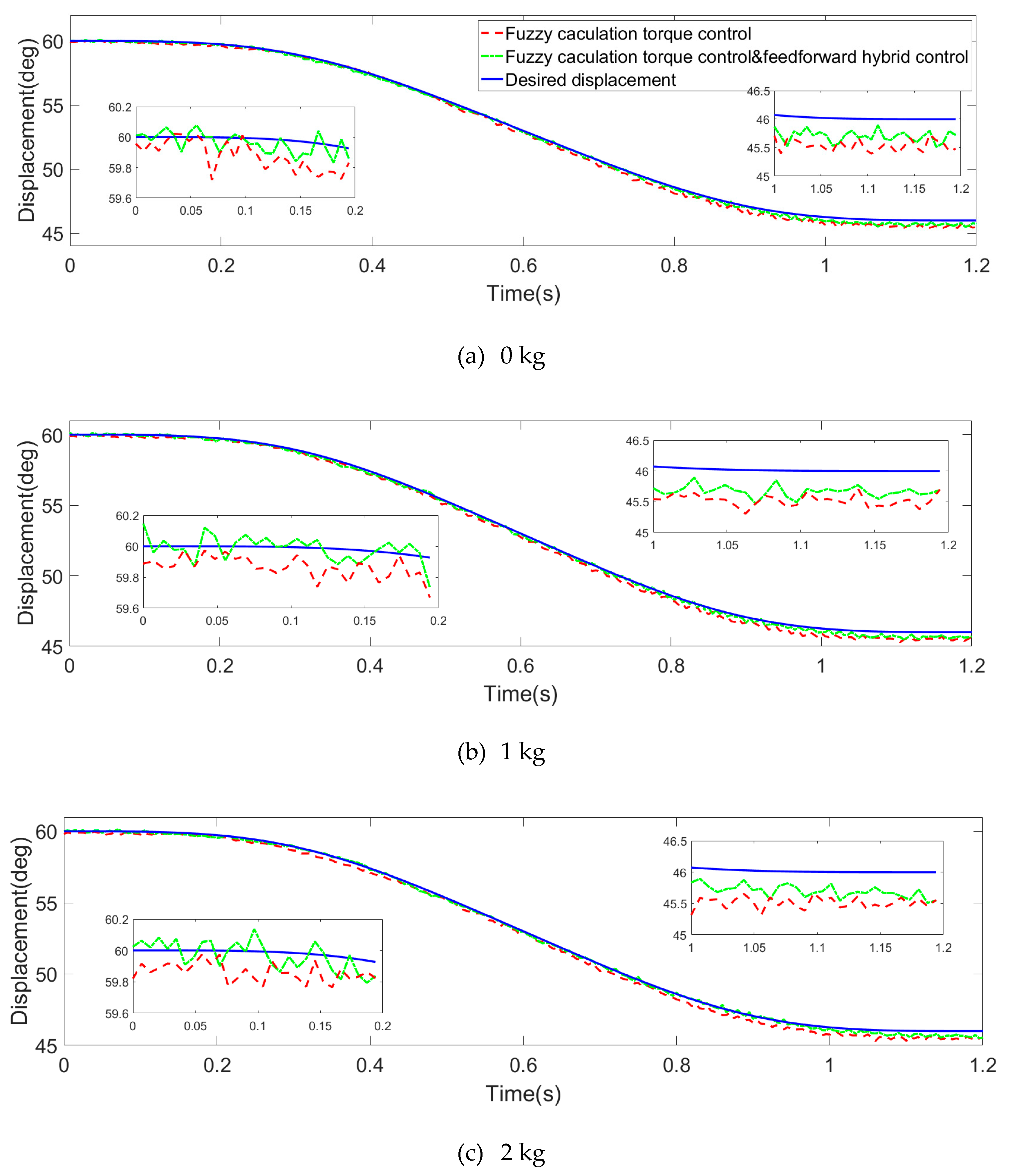
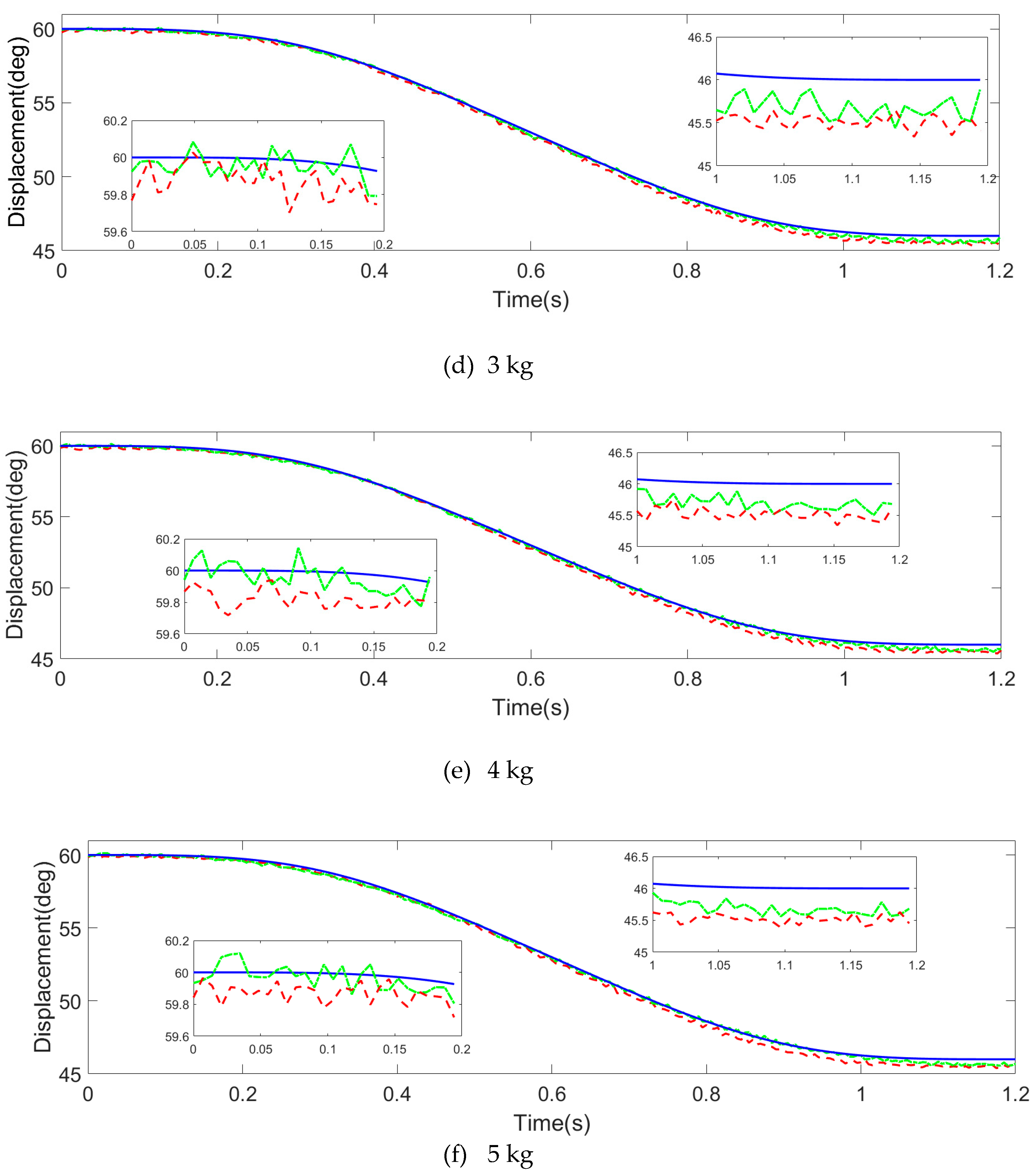
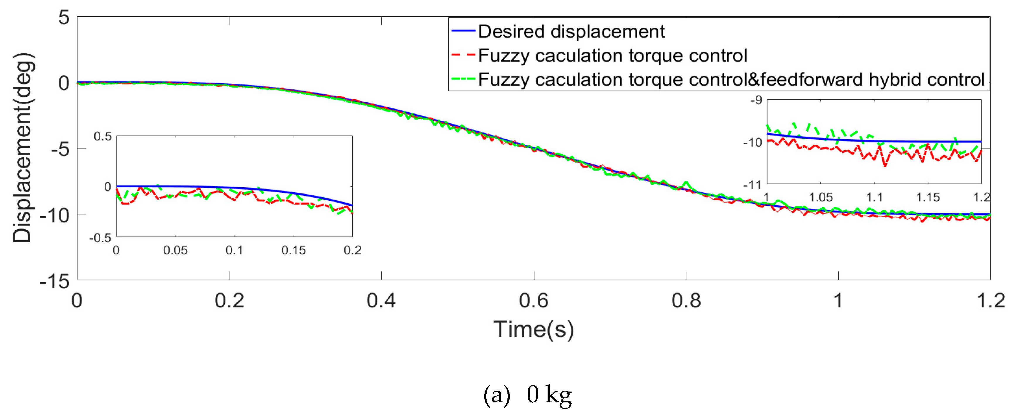
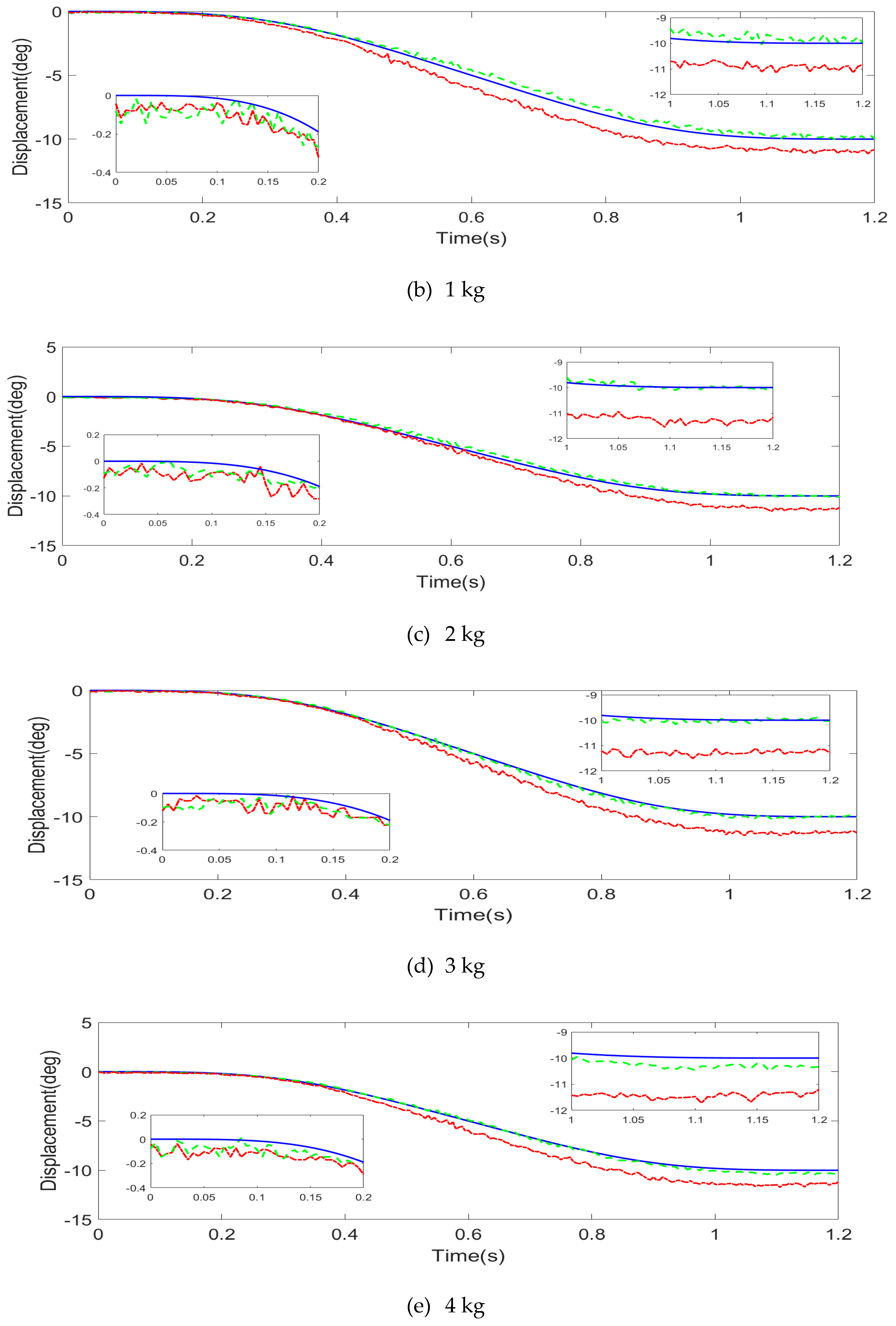
• When the robot’s joints move under variable load, compared with the fuzzy computational torque feedback, the fuzzy computational torque feedback and torque feedforward hybrid control decreased the RMS values of tracking errors by 49.87%, 70.48%, and 50.37%, respectively, and increased the kinematic precision at the same time.
• Compared with simple torque feedback control, the hybrid torque control increased the velocity stability by 23.35%, 17.66%, and 25.04%, respectively; that is, the velocity stability of the hybrid torque control method was better than only the feedback torque control method.

References

1. Wang, B.; Qi, Z.; Yan, R.; Liu, H.Q. Dynamic Parameter Identification of SCARA Robot Based on Stochastic Weighted Particle Swarm Optimization. J. Xi’an Jiaotong Univ. 2021, 55, 20–27. [Google Scholar]
2. Cazalilla, J.; Vallés, M.; Mata, V.; Díaz-Rodríguez, M.; Valera, A. Adaptive control of a 3-DOF parallel manipulator considering payload handling and relevant parameter models. Robot. Comput. Integr. Manuf. 2014, 30, 468–477. [Google Scholar] [CrossRef]
3. Lee, K.W.; Khalil, H.K. Adaptive output feedback control of robot manipulators using high-gain observer. Int. J. Control 1997, 67, 869–886. [Google Scholar] [CrossRef]
4. Binbin, D.; Ling, Q.; Wang, S. Improvement of the conventional computed-torque control scheme with a variable structure compensator for delta robots with uncertain load. In Proceedings of the 2014 International Conference on Mechatronics and Control (ICMC), Jinzhou, China, 3–5 July 2014. [Google Scholar]
5. Nguyen, V.T.; Su, S.F.; Wang, N.; Sun, W. Adaptive finite-time neural network control for redundant parallel manipulators. Asian J. Control 2020, 22, 2534–2542. [Google Scholar] [CrossRef]
6. Zhang, H.; Fang, H.; Zhang, D.; Luo, X.; Zou, Q. Fuzzy sliding mode control for a 3-DOF parallel manipulator with parameters uncertainties. Complexity 2020, 2020, 2565316. [Google Scholar] [CrossRef] [Green Version]
7. Zhang, Y.; Li, Y.; Zhang, S. Adaptive neural dynamic surface control of robot manipulators with unknown loads. IEEE Trans. Ind. Electron. 2019, 67, 2332–2342. [Google Scholar]
8. Lin, J.; Tan, J.; Xue, J.; Liu, G. Robust adaptive neural network control of robot manipulators with uncertain loads. IEEE Trans. Neural Netw. Learn. Syst. 2018, 29, 1004–1014. [Google Scholar]
9. Hu, S.; Kang, H.; Tang, H.; Cui, Z.; Liu, Z.; Ouyang, P. Trajectory Optimization Algorithm for a 4-DOF Redundant Parallel Robot Based on 12-Phase Sine Jerk Motion Profile. Actuators 2021, 10, 80. [Google Scholar] [CrossRef]
10. Do Thanh, T.; Kotlarski, J.; Heimann, B.; Ortmaier, T. Dynamics identification of kinematically redundant parallel robots using the direct search method. Mech. Mach. Theory 2012, 52, 277–295. [Google Scholar] [CrossRef]
11. Gao, L.; Yuan, J.; Han, Z.; Wang, S.; Wang, N. A friction model with velocity, temperature and load torque effects for collaborative industrial robot joints. In Proceedings of the 2017 IEEE/RSJ International Conference on Intelligent Robots and Systems (IROS), Vancouver, BC, Canada, 24–28 September 2017. [Google Scholar]
12. Simoni, L.; Villagrossi, E.; Beschi, M.; Marini, A.; Pedrocchi, N.; Tosatti, L.M.; Visioli, A. On the Use of a Temperature Based Friction Model for a Virtual Force Sensor in Industrial Robot Manipulators. In Proceedings of the 2017 22nd IEEE International Conference on Emerging Technologies and Factory Automation (ETFA), Limassol, Cyprus, 12–15 September 2017. [Google Scholar]
13. Jalon, D.; Garcia, J.; Bayo, E. Kinematic and Dynamic Simulation of Multibody Systems: The Real-Time Challenge; Springer: Berlin/Heidelberg, Germany, 2012. [Google Scholar]
14. Abbasimoshaei, A.; Mohammadimoghaddam, M.; Kern, T.A. Adaptive fuzzy sliding mode controller design for a new hand rehabilitation robot. In Proceedings of the Haptics: Science, Technology, Applications: 12th International Conference, EuroHaptics 2020, Leiden, The Netherlands, 6–9 September 2020; Springer International Publishing: Cham, Switzerland, 2020. [Google Scholar]
15. Dong, L.; Tao, T.; Xuesong, M.; Dongsheng, Z. Decoupling identification method for linear characteristics and nonlinear friction of servo system. Chin. J. Sci. Instrum. 2010, 31, 782–788. [Google Scholar]
16. Wu, X.; Liu, D.; He, M.; Gao, F.; Shao, G. Research on Modeling and Compensation of robot joint Friction. J. Instrum. 2018, 39, 44–50. [Google Scholar] [CrossRef]
17. Kim, T.J.; Ahn, K.H.; Song, J.B. Friction Model of a Robot Joint Considering Torque and Moment Loads. Trans. Korean Soc. Mech. Eng. A 2021, 45, 27–34. [Google Scholar] [CrossRef]
18. Wen, S. Tribology Principle; Tsinghua University Press: Beijing, China, 1990; pp. 7–11. [Google Scholar]
19. Choi, J.H.; Sehoon, O.; Jinung, A. Sensorless Force Control with Observer for Multi-functional Upper Limb Rehabilitation Robot. J. Korea Robot. Soc. 2017, 12, 356–364. [Google Scholar] [CrossRef]
20. Roveda, L.; Pallucca, G.; Pedrocchi, N.; Braghin, F.; Tosatti, L.M. Iterative learning procedure with reinforcement for high-accuracy force tracking in robotized tasks. IEEE Trans. Ind. Inform. 2017, 14, 1753–1763. [Google Scholar] [CrossRef]
21. Hajnayeb, A.; Ghasemloonia, A. Nonparametric Identification of the Surgeon’s Hand Vibration in Haptic Devices. In Proceedings of the 2018 23rd International Conference on Methods & Models in Automation & Robotics (MMAR), Miedzyzdroje, Poland, 27–30 August 2018. [Google Scholar]
22. Zubizarreta, A.; Marcos, M.; Cabanes, I.; Pinto, C.; Portillo, E. Redundant sensor based control of the 3RRR parallel robot. Mech. Mach. Theory 2012, 54, 1–17. [Google Scholar] [CrossRef]
23. Serdar, K. Energy minimization for 3-RRR fully planar parallel manipulator using particle swarm optimization. Mech. Mach. Theory 2013, 62, 129–149. [Google Scholar]
24. Harandi MR, J.; Khalilpour, S.A.; Taghirad, H.D.; Romero, J.G. Adaptive control of parallel robots with uncertain kinematics and dynamics. Mech. Syst. Signal Process. 2021, 157, 107693. [Google Scholar] [CrossRef]
25. Moshaii, A.A.; Moghaddam, M.M.; Niestanak, V.D. Fuzzy sliding mode control of a wearable rehabilitation robot for wrist and finger. Ind. Robot. Int. J. Robot. Res. Appl. 2019, 46, 839–850. [Google Scholar] [CrossRef]
26. Abbasi Moshaei, A.R.; Mohammadi Moghaddam, M.; Dehghan Neistanak, V. Analytical model of hand phalanges desired trajectory for rehabilitation and design a sliding mode controller based on this model. Modares Mech. Eng. 2020, 20, 129–137. [Google Scholar]
27. Wenxiang, W.; Shiqiang, Z.; Xuanyin, W.; Huashan, L. Robot low speed control based on friction fuzzy modeling and compensation. Electr. Mach. Control. 2013, 17, 70–77. [Google Scholar]
Figure 1. Overall structure diagram of a 4-DOF redundant parallel robot. (a) Structure diagram of a 4-DOF redundant parallel robot: (1) Pedestal; (2) Driving shaft; (3) Driven shaft; (4) Air gripper; (5) End effector. (b) Construction of coordinate system for 4-DOF redundant Parallel Robot.
Actuators 12 00232 g001
Figure 2. Simplified schematic diagram of the single-chain mechanism.
Actuators 12 00232 g002
Figure 3. Torque control structure diagram.
Actuators 12 00232 g003
Figure 4. Feedforward controller structure diagram.
Actuators 12 00232 g004
Figure 5. Feedback controller structure diagram using a combination of computational torque control and fuzzy control to feedback the robot’s traveling torque.
Actuators 12 00232 g005
Figure 6. Membership function of fuzzy controller.
Actuators 12 00232 g006
Figure 7. Comparison of friction torque measurement and identification results.
Actuators 12 00232 g007
Figure 8. Feedforward compensation torque diagram of each drive joint under variable load: (a) Joint 1; (b) Joint 3; (c) Joint 5.
Actuators 12 00232 g008
Figure 9. Loading experiment diagram. (a) 4-DOF redundant parallel robot structure diagram. (b) Loading external load experiment diagram.
Actuators 12 00232 g009
Figure 10. Comparison of angular displacements of joint 1 under different external loads with and without torque feedforward compensation control.
Actuators 12 00232 g010aActuators 12 00232 g010b
Figure 11. Comparison of angular displacements of joint 2 under different external loads with and without torque feedforward compensation control.
Actuators 12 00232 g011aActuators 12 00232 g011bActuators 12 00232 g011c
Figure 12. Comparison of angular displacements of joint 3 under different external loads with and without torque feedforward compensation control.
Actuators 12 00232 g012aActuators 12 00232 g012b
Figure 13. The comparison of the root of tracking error of joint 1 under variable load between torque feedback and torque feedforward and feedforward hybrid control.
Actuators 12 00232 g013
Figure 14. The comparison of the root of tracking error of joint 3 under variable load between torque feedback and torque feedforward and feedforward hybrid control.
Actuators 12 00232 g014
Figure 15. The comparison of the root of tracking error of joint 5 under variable load between torque feedback and torque feedforward and feedforward hybrid control.
Actuators 12 00232 g015
Figure 16. Comparison of the angular velocity of joint 1 under different external loads with and without torque feedforward compensation control.
Actuators 12 00232 g016aActuators 12 00232 g016b
Figure 17. Comparison of the angular velocity of joint 2 under different external loads with and without torque feedforward compensation control.
Actuators 12 00232 g017aActuators 12 00232 g017b
Figure 18. Comparison of the angular velocity of joint 3 under different external loads with and without torque feedforward compensation control.
Actuators 12 00232 g018aActuators 12 00232 g018b
Figure 19. Speed stability analysis of torque feedforward and feedback and feedback under the variable load of joint 1.
Actuators 12 00232 g019
Figure 20. Speed stability analysis of torque feedforward and feedback and feedback under the variable load of joint 3.
Actuators 12 00232 g020
Figure 21. Speed stability analysis of torque feedforward and feedback and feedback under the variable load of joint 5.
Actuators 12 00232 g021