Extended State Observer-Based Sliding Mode Control Design of Two-DOF Lower Limb Exoskeleton

Abstract

Due to some model uncertainties and unknown friction disturbances that exist in the 2-DOF lower limb exoskeleton, a linear extended state observer (LESO) is proposed to estimate the unmeasurable angular velocity of two joints and the lumped uncertainties caused by friction disturbance and hydraulic parametric uncertainties. Meanwhile, by using the Lyapunov technique, a sliding mode controller is designed to improve the dynamic performance and the steady state accuracy of two joint angle responses in human–exoskeleton cooperative motion. By regulating the sliding mode controller gain, both the system state errors and estimation errors of the LESO are reduced in an arbitrary boundary of zero neighborhood. Finally, the effectiveness of the proposed control scheme is verified with both simulation and experimental results for one operator-wearable test, to guarantee that the joint position tracking performance and human–exoskeleton impedance torques are suppressed in a satisfactory boundary.

1. Introduction

Wearable electromechanical technology has been rapidly developed in recent years. As a typical wearable system device, exoskeleton robots are applied in many biological and medical engineering fields [1,2,3,4]. In fact, exoskeletons assist patients with finishing many rehabilitation training tasks, which efficiently reduces the work burden of care workers and improves the rehabilitation of hemiplegic patients. Secondly, exoskeletons can help the elder population with some daily behaviors such as walking or going up and down stairs. Moreover, some exoskeleton boots enhance transportation power for travelling long distances, used by, for example, logistics laborers and soldiers. Therefore, wearable exoskeletons have obvious applications for improving individuals’ quality of life.

An exoskeleton robot generally includes a mechanical plant, electronic controllers, i.e., displacement sensors, human–exoskeleton interaction force/torque sensors, AD/DA conversion, etc. The lower extremity exoskeleton developed by Berkeley (BLEEX) is the first human exoskeleton that was widely demonstrated to walk energetically and autonomously while supporting its own weight and an external payload [5]. Then, a high-energy-density actuation was used in a self-powered position-or force-controlled human-scale robot to verify the effectiveness of the force-control approach [6]. Most exoskeletons are driven by both motors and electrohydraulics with different motion control modes. An adaptive control scheme incorporating learning control approaches into the exoskeleton system was developed to help the exoskeleton’s leg movement along a desired periodic trajectory and to handle periodic uncertainties with known periods [7]. Then, a variable admittance controller [8] was designed to reduce real-time human–exoskeleton interaction torque based on the gait prediction uncertainties quantified by the deep-Gaussian process method. Meanwhile, to address the randomness and uncertainty of individual walking gaits, an output constrained control of a lower limb exoskeleton based on a knee motion probabilistic model with finite-time extended state observer was developed [9]. On the other hand, a repetitive learning control is used in a lower limb exoskeleton driven by electrohydraulic actuators to compensate the large external loads of two mechanical legs [10]. Similarly, a feedback control law was designed in the frequency domain to achieve cylinder position tracking and guarantee the aid-force effect of the exoskeleton, which had more than 70% aid-force efficiency in the walking stance phase [11]. For example, an adaptive fuzzy control is proposed in [12,13] to estimate uncertain parameters and unmodeled uncertainties of the wearable exoskeleton. Although some software designed using CAD and Creo can calculate many rough mechanical structure parameters, such as the center of mass, moment of inertia, and the friction damping, the machining and manufacturing will generate many structure errors. Hence, it is difficult to obtain the accurate dynamic model parameters of exoskeleton robots due to their irregular structure.

To enhance the robust and output performance of the exoskeleton, many state-of-the-art controllers have been presented such as adaptive fuzzy control [12], repetitive learning control [10], RBFNN adaptive control [14], and discrete-time ESO-based intelligent PD control [15]. The exoskeleton generally has active and passive motion control modes [16]. For the passive mode, the joint trajectory demand is roughly designed, which does not reflect the operator’s motion intention in real time [17]. A suitable control algorithm is designed for assistant training and rehabilitation of the ankle joint in the presence of musculoskeletal injuries [18]. Meanwhile, an admittance control technique is employed to perform patient-active exercises with and without motion assistance. Furthermore, an adaptive backstepping control is constructed to improve the dynamic tracking performance of the human–robot training mode in the presence of the identification error [19]. Similarly, an adaptive impedance control is used in networked Lagrangian systems to simulate typical robot–environment interactions [20]. However, in the active mode, the joint trajectory demand is designed based on the human–exoskeleton interaction force/torque. The impedance and admittance controllers [21] are often used to maximally reduce the compliance between the operator and the exoskeleton. Li et al. [22] adopted admittance control to address the operator’s intention in human–exoskeleton cooperative motion. Yu et al. [23] presented an adaptive impedance control to improve the performance in the case of some dynamic uncertainties. Meanwhile, some model-based controllers and model-free controllers are also studied in exoskeletons. Many model-based control methods have been proposed for the 2-DOF robotic manipulator. For instance, neural adaptive control is used in a single-rod electrohydraulic system with lumped uncertainty [24]. Then, a neural adaptive backstepping control is adopted in a robotic manipulator with a prescribed performance constraint [25]. A model-free controller, such as PID, finds it difficult to hold a satisfactory performance under parametric uncertainty and external load disturbance. However, the synthesized performance and stability of model-based controller is usually determined by the modeling accuracy. Hence, the popular adaptive backstepping controller has been presented to handle model uncertainties in many fields such as a wheeled mobile robot [26], the Quadrotor [27], and the Euler–Bernoulli beam [28]. Generally, a favor controller should address not only parametric uncertainties and unknown external disturbances, but also some unmeasurable state feedback problems. The above-mentioned control methods cannot solve all issues in human–exoskeleton cooperative motion.

There are two typical problems with exoskeleton motion control, i.e., stability and safety. At first, many uncertainties and disturbances will lead to instability of the system and cause the operator to be unsafe [29]. Hence, much work has been proposed to address this issue, such as fuzzy adaptive control [30,31], NN adaptive control [32], iterative learning control [10,33], disturbance observer [15,22,34], etc. Meanwhile, the extended state observer estimates unknown state and external disturbances in practice, for marine surface vehicles [35] such as autonomous underwater vehicles [36], turret-moored vessels [37], electrohydraulic systems [24], etc. For the inherent physical constraints of the human–exoskeleton plant, references [32,33] present the corresponding constraint control strategies for both upper and lower limb exoskeletons. Wu et al. presented a soft elbow exoskeleton for the rehabilitation training of disabled patients [38] and developed a minimal intervention-based admittance control strategy for an upper extremity rehabilitation exoskeleton [39]. Inspired by the previous work on the extended state observer mentioned in [40] and the sliding mode control proposed in [41], the passive control of human–exoskeleton cooperative motion is studied to improve the tracking performance of the exoskeleton.

In fact, the active control mode of the exoskeleton focuses on decreasing the human–exoskeleton impedance rather than the joint demand tracking error [42]. It should be noted that, different from the variable admittance strategy adopted in [8], this study presents an extended state observer-based sliding mode control scheme in the passive control mode of a 2-DOF lower limb exoskeleton. Furthermore, the previous work in [43] has only realized a rough simulation of the active control mode of an exoskeleton, and has carried out experimental verification in human-cooperative motion. In this study, both the joint position tracking performance and the human–exoskeleton interaction torques of two joints are demonstrated to verify the effectiveness of the proposed control scheme. To be honest, the extended state observer is used not only to estimate the isolated disturbance input but also to compensate for general dynamics, which includes nonmodelled dynamics [44,45]. Hence, the main contributions are as follows:

(I)

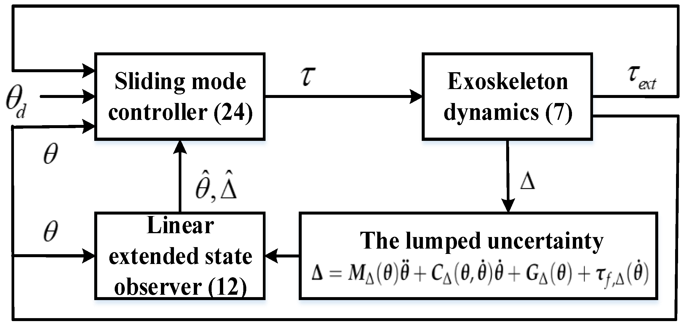
A linear extended state observer (LESO) is used to estimate the unmeasurable angular velocity of two joints and the model uncertainties in the exoskeleton Lagrangian model, which can avoid the numerical differentiation of the encoder data for the angular velocity estimation. In fact, the LESO is a high-gain observer that guarantees a satisfactory estimation error in the exoskeleton inner-loop by regulating the observer bandwidth.

(II)

A sliding mode controller is designed to improve the tracking performance of the passive control mode of human–exoskeleton cooperative motion under model uncertainties and the unknown angular velocity of the exoskeleton. Meanwhile, the sliding mode controller guarantees that the joint tracking error converges to a small-enough zero neighborhood by regulating the control gains, which is easily realized in the experimental bench.

The remainder of this paper is organized as follows. The exoskeleton dynamic model is described in Section 2. The LESO of the exoskeleton is designed in Section 3. Then, the sliding mode controller is given in Section 4. Both simulation and experimental verification are given in Section 5 and Section 6. Finally, the conclusions are drawn in Section 8.

2. Exoskeleton Dynamic Model

The lower limb exoskeleton is a portable carrier that effectively realizes human–machine cooperative motion, which requires a humanoid mechanical structure and an actuator with a high power density to guarantee a fast response to the operator’s motion intention. The mechanical structure of the exoskeleton is formed of aluminum material as shown in Figure 1, and the corresponding mechanical parameters are given in

Table 1. The mechanical parameters of 2-DOF lower limb exoskeleton.

Parameter	Symbol	Parameter	Symbol
Thigh weight	$m_{th}$	Shank weight	$m_{sh}$
Thigh length	$a_{th}$	Shank length	$a_{sh}$
Thigh centroid length	$l_{th}$	Shank centroid length	$l_{sh}$
Thigh moment of inertia	$I_{th}$	Shank moment of inertia	$I_{sh}$

. It is one humanoid leg with two degrees of freedom. The mechanical frame is fixed on the ground, and the exoskeleton joint has a fixed connection to the frame. Two hip and knee joints are driven by disc motors. Then, four three-dimensional (3D) force sensors are installed on two exoskeleton legs to measure human–exoskeleton interaction torque as an operator’s leg wrap bandage. The two joint angles are measured by absolute encoders fixed on the hip and knee, respectively.

Remark 1.

Considering the passive control mode of human–exoskeleton cooperative motion, the human leg dynamics is neglected and the human–exoskeleton impedance is regarded as the external disturbance of the exoskeleton dynamic model.

By using the Lagrangian technique, the dynamic model of the 2-DOF lower limb exoskeleton is constructed as follows [46]:

$$M\left(\theta \right)\ddot{\theta }+C(\theta ,\dot{\theta })\dot{\theta }+\mathit{G}\left(\theta \right)+{\tau }_f\left(\dot{\theta }\right)=\tau +{\tau }_{ext},$$

(1)

where $\theta \in {\mathbb{R}}^2$ is the joint angle, $\tau \in {\mathbb{R}}^2$ is the motor torque driven, ${\mathit{\tau }}_{ext}=J^T\left(\theta \right)F_{ext}$ is the human–exoskeleton interaction torque, $J^T\left(\theta \right)\in {\mathbb{R}}^{2\times 2}$ is the Jacobian matrix, and $F_{ext}\in {\mathbb{R}}^2$ is the human–exoskeleton interaction force, and ${\tau }_f\left(\dot{\theta }\right)$ is the friction disturbance, $M\left(\theta \right)\in {\mathbb{R}}^{2\times 2}$, $\mathit{C}(\theta ,\dot{\theta })\in {\mathbb{R}}^{2\times 2}$, and $G\left(\theta \right)\in {\mathbb{R}}^2$ are the inertia matrix, Coriolis torque, and gravity force, respectively.

The Lagrangian model functions are given by

$$M\left(\theta \right)=\left[\begin{array}{cc}\begin{array}{c}{I}_{th}+I_{sh}+m_{th}{l}_{th}^2\hfill \\ +m_{sh}{a}_{th}^2+m_{sh}{l}_{sh}^2\hfill \\ +2m_{sh}{a}_{th}{l}_{sh}cos{\theta }_2\hfill \end{array}& \begin{array}{c}{I}_{sh}+m_{sh}{l}_{sh}^2\hfill \\ +m_{sh}{a}_{th}{l}_{sh}cos{\theta }_2\hfill \end{array}\\ \begin{array}{c}{I}_{sh}+m_{sh}{l}_{sh}^2\hfill \\ +m_{sh}{a}_{th}{l}_{sh}cos{\theta }_2\hfill \end{array}& I_{sh}+m_{sh}{l}_{sh}^2\end{array}\right],$$

(2)

$$C(\theta ,\dot{\theta })=\left[\begin{array}{cc}-m_{sh}{a}_{th}{l}_{sh}sin{\theta }_2{\dot{\theta }}_2& -m_{sh}{a}_{th}{l}_{sh}sin{\theta }_2({\dot{\theta }}_1+{\dot{\theta }}_2)\\ m_{sh}{a}_{th}{l}_{sh}sin{\theta }_2{\dot{\theta }}_1& 0\end{array}\right],$$

(3)

$$G\left(\theta \right)=\left[\begin{array}{c}{l}_{th}{m}_{th}gsin{\theta }_1+m_{sh}g(a_{th}sin{\theta }_1+l_{sh}sin({\theta }_1+{\theta }_2))\\ l_{sh}{m}_{sh}gsin({\theta }_1+{\theta }_2)\end{array}\right],$$

(4)

where ${\dot{\theta }}_i,{\ddot{\theta }}_i(i=1,2)$ are the angular velocity and acceleration of exoskeleton two joints, respectively; $I_i(i=1,2)$ are the moment of inertia of thigh and shank, respectively.

The friction disturbance ${\tau }_f\left(\dot{\theta }\right)$ is described as

$${\tau }_f\left(\dot{\theta }\right)=\left[\begin{array}{c}{b}_{1,1}\mathrm{sgn}\left({\dot{\theta }}_1\right)+b_{1,2}{\dot{\theta }}_1\\ b_{2,1}\mathrm{sgn}\left({\dot{\theta }}_2\right)+b_{1,2}{\dot{\theta }}_2\end{array}\right],$$

(5)

where $b_{i,1},b_{i,2}(i=1,2)$ are the Coulomb and viscous friction coefficients, respectively.

Assumption 1.

Due to some model uncertainties and unknown friction disturbance existing in the exoskeleton, the Lagrangian model functions are described as follows:

$$\left\{\begin{array}{c}\begin{array}{cc}\hfill M\left(\theta \right)& =M_0\left(\theta \right)+M_{\Delta }\left(\theta \right)\hfill \\ \hfill C(\theta ,\dot{\theta })& =C_0(\theta ,\dot{\theta })+C_{\Delta }(\theta ,\dot{\theta })\hfill \\ \hfill G\left(\theta \right)& =G_0\left(\dot{\theta }\right)+G_{\Delta }\left(\dot{\theta }\right)\hfill \\ \hfill {\tau }_f\left(\dot{\theta }\right)& ={\tau }_{f,0}\left(\dot{\theta }\right)+{\tau }_{f,}\left(\dot{\theta }\right),\hfill \end{array}\end{array}\right.$$

(6)

where $M_0\left(\theta \right)$, $C_0(\theta ,\dot{\theta })$, $G_0\left(\dot{\theta }\right)$ are the nominal and known functions, and $M_{\Delta }\left(\theta \right)$, $C_{\Delta }(\theta ,\dot{\theta })$, $G_{\Delta }\left(\dot{\theta }\right)$ are unknown functions.

Hence, (1) can be rewritten as

$$M_0\left(\theta \right)\ddot{\theta }+C_0(\theta ,\dot{\theta })\dot{\theta }+G_0\left(\theta \right)+{\tau }_{f,0}\left(\dot{\theta }\right)+\Delta =\tau +{\tau }_{ext},$$

(7)

where $\Delta =M_{\Delta }\left(\theta \right)\ddot{\theta }+C_{\Delta }(\theta ,\dot{\theta })\dot{\theta }+G_{\Delta }\left(\theta \right)+{\tau }_{f,\Delta }\left(\dot{\theta }\right)$ is the lumped uncertainty.

3. Linear ESO Design

If the state variables $q={[q_1,q_2]}^T={[\theta ,\dot{\theta }]}^T$, then the state space model of the 2-DOF lower limb exoskeleton is

$$\left\{\begin{array}{c}\begin{array}{cc}\hfill {\dot{q}}_1& =q_2\hfill \\ \hfill {\dot{q}}_2& =M_0^{-1}\left(\tau +{\tau }_{ext}-C_0{q}_2-G_0-{\tau }_{f,0}\right)-M_0^{-1}\Delta .\hfill \end{array}\hfill \end{array}\right..$$

(8)

If an extended state variable is defined as $q_3=M_0^{-1}\Delta$, then (8) is converted into

$$\left\{\begin{array}{c}\begin{array}{cc}\hfill {\dot{q}}_1& =q_2\hfill \\ \hfill {\dot{q}}_2& =M_0^{-1}\left[\tau +{\tau }_{ext}-\phi \left(q\right)-G_0\right]-q_3\hfill \\ \hfill {\dot{q}}_3& =\delta \left(t\right),\hfill \end{array}\hfill \end{array}\right.$$

(9)

where $\delta \left(t\right)$ is the time derivative of $q_3$, $\phi \left(q\right)=C_0{q}_2+{\tau }_{f,0}$.

Assumption 2.

The function $\phi \left(q\right)$ is Lipschitz with respect to $q_2$, while the lumped uncertainty Δ and its time derivative $\dot{\Delta }$ are both bounded.

Since the angular velocity $\dot{\theta }$ is unmeasured, q${}_2$ is unknown. Hence, the LESO should estimate both q${}_2$ and q${}_3$, which is compensated in the controller design. The augmented system (9) is rewritten as

$$\dot{q}=A_{0}q+B_{0}u+B_0({\tau }_{ext}-G_0)-\Phi \left(q\right)+D\left(t\right),$$

(10)

where

$$\begin{array}{c}{A}_0=\left[\begin{array}{ccc}{0}_{2\times 2}& -I_{2\times 2}& 0_{2\times 2}\\ 0_{2\times 2}& 0_{2\times 2}& -I_{2\times 2}\\ 0_{2\times 2}& 0_{2\times 2}& 0_{2\times 2}\end{array}\right]B_0=\left[\begin{array}{c}{0}_{2\times 2}\\ M_0^{-1}\left(q\right)\\ 0_{2\times 2}\end{array}\right]\hfill \\ \Phi \left(q\right)=\left[\begin{array}{c}{0}_{2\times 1}\\ M_0^{-1}\left(q\right)\phi \left(q\right)\\ 0_{2\times 1}\end{array}\right]D\left(t\right)=\left[\begin{array}{c}{0}_{2\times 1}\\ 0_{2\times 1}\\ \delta \left(t\right)\end{array}\right]\hfill \end{array},$$

(11)

and $I_{2\times 2}$ and $0_{2\times 2}$ are two unit matrices.

Then, the LESO is designed as

$$\dot{\hat{q}}=A_0\hat{q}+B_{0}u+B_0({\tau }_{ext}-G_0)-\hat{\Phi }\left(\hat{q}\right)+H(q_1-{\hat{q}}_1),$$

(12)

where $\hat{\Phi }\left(\hat{q}\right)=\Phi (q_1,{\hat{q}}_2)$, and $H={[3{\omega }_0,3{\omega }_0^2,{\omega }_0^3]}^T\otimes I_{2\times 2}$ is the observer gain and ${\omega }_0$ is the observer bandwidth.

From (10) and (12), we can obtain that

$$\dot{\tilde{q}}=A_0\tilde{q}-\tilde{\Phi }\left(\hat{q}\right)+D\left(t\right)+H(q_1-{\hat{q}}_1),$$

(13)

where $\tilde{\Phi }\left(\hat{q}\right)=\Phi \left(q_1,q_2\right)-\hat{\Phi }(q_1,{\hat{q}}_2)$.

Theorem 1.

Consider the LESO (12) under Assumption 2; the state estimation errors ${\tilde{q}}_i=q_i-{\hat{q}}_i(i=1,2,3)$ converge to a small-enough zero neighborhood.

Proof. 

Let $\epsilon ={[{\epsilon }_1,{\epsilon }_2,{\epsilon }_3]}^T$, where ${\epsilon }_1={\tilde{q}}_1$, ${\epsilon }_2={\tilde{q}}_2/{\omega }_0$, ${\epsilon }_3={\tilde{q}}_3/{\omega }_0^2$ are defined as the scaled estimation error, then (13) is converted into

$$\dot{\epsilon }={\omega }_{0}A\epsilon -B_2\frac{M_0^{-1}\tilde{\phi }\left(q\right)}{{\omega }_0}+B_3\frac{\delta \left(t\right)}{{\omega }_0^2},$$

(14)

where

$$\begin{array}{c}A=\left[\begin{array}{ccc}-3I_{2\times 2}& I_{2\times 2}& 0_{2\times 2}\\ -3I_{2\times 2}& 0_{2\times 2}& I_{2\times 2}\\ -I_{2\times 2}& 0_{2\times 2}& 0_{2\times 2}\end{array}\right],\hfill \\ B_2=\left[\begin{array}{c}{0}_{2\times 2}\\ I_{2\times 2}\\ 0_{2\times 2}\end{array}\right],B_3=\left[\begin{array}{c}{0}_{2\times 2}\\ 0_{2\times 2}\\ I_{2\times 2}\end{array}\right]\hfill \end{array}.$$

(15)

Based on the selection rule of the observer bandwidth ${\omega }_0$ in ref. [47], the matrix A is Hurwitz. There exists a positive definite matrix P such that

$$A^{T}P+PA=-2I.$$

(16)

Hence, the positive definite Lyapunov function of the estimation error dynamics (14) is selected as follows:

$$V_{\epsilon }={\epsilon }^{T}P\epsilon .$$

(17)

Then, the time derivative of $V_{\epsilon }$ yields that

$$\begin{array}{c}\begin{array}{cc}\hfill {\dot{V}}_{\epsilon }& ={\dot{\epsilon }}^{T}P\epsilon +{\epsilon }^{T}P\dot{\epsilon }\hfill \\ \hfill & ={\omega }_0({\epsilon }^T{A}^{T}P\epsilon +{\epsilon }^{T}PA\epsilon )+{(B_3\frac{\delta }{{\omega }_0^2}-B_2\frac{M_0^{-1}\tilde{\phi }}{{\omega }_0})}^{T}P\epsilon \hfill \\ \hfill & +{\epsilon }^{T}P(B_3\frac{\delta }{{\omega }_0^2}-B_2\frac{M_0^{-1}\tilde{\phi }}{{\omega }_0})\hfill \end{array}\end{array}.$$

(18)

According to Assumption 2, we have $\tilde{\phi }\left(q\right)<\alpha \epsilon$, and ${\dot{V}}_{\epsilon }$ satisfies that

$${\dot{V}}_{\epsilon }\le 2\left(\frac{{\gamma }_1\alpha }{{\omega }_0}∥M_0^{-1}∥-{\omega }_0\right){∥\epsilon ∥}^2+\frac{2{\gamma }_2}{{\omega }_0^2}\left|\delta \right|∥\epsilon ∥,$$

(19)

where ${\gamma }_1=∥P{B}_2∥$, ${\gamma }_2=∥P{B}_3∥$.

Hence, (19) indicates that

$$\mathrm{if}∥\epsilon ∥\ge \frac{{\gamma }_2\left|\delta \right|}{{\omega }_0\left({\omega }_0^2-{\gamma }_1\alpha ∥M_0^{-1}∥\right)},\mathrm{then}{\dot{V}}_{\epsilon }\le 0.$$

(20)

Based on (20) and the definition of the scaled estimation error $\epsilon$, the state estimation errors ${\tilde{q}}_i=q_i-{\hat{q}}_i(i=1,2,3)$ converge to an arbitrarily small zero neighborhood by largely regulating the observer bandwidth ${\omega }_0$. □

4. Sliding Mode Control

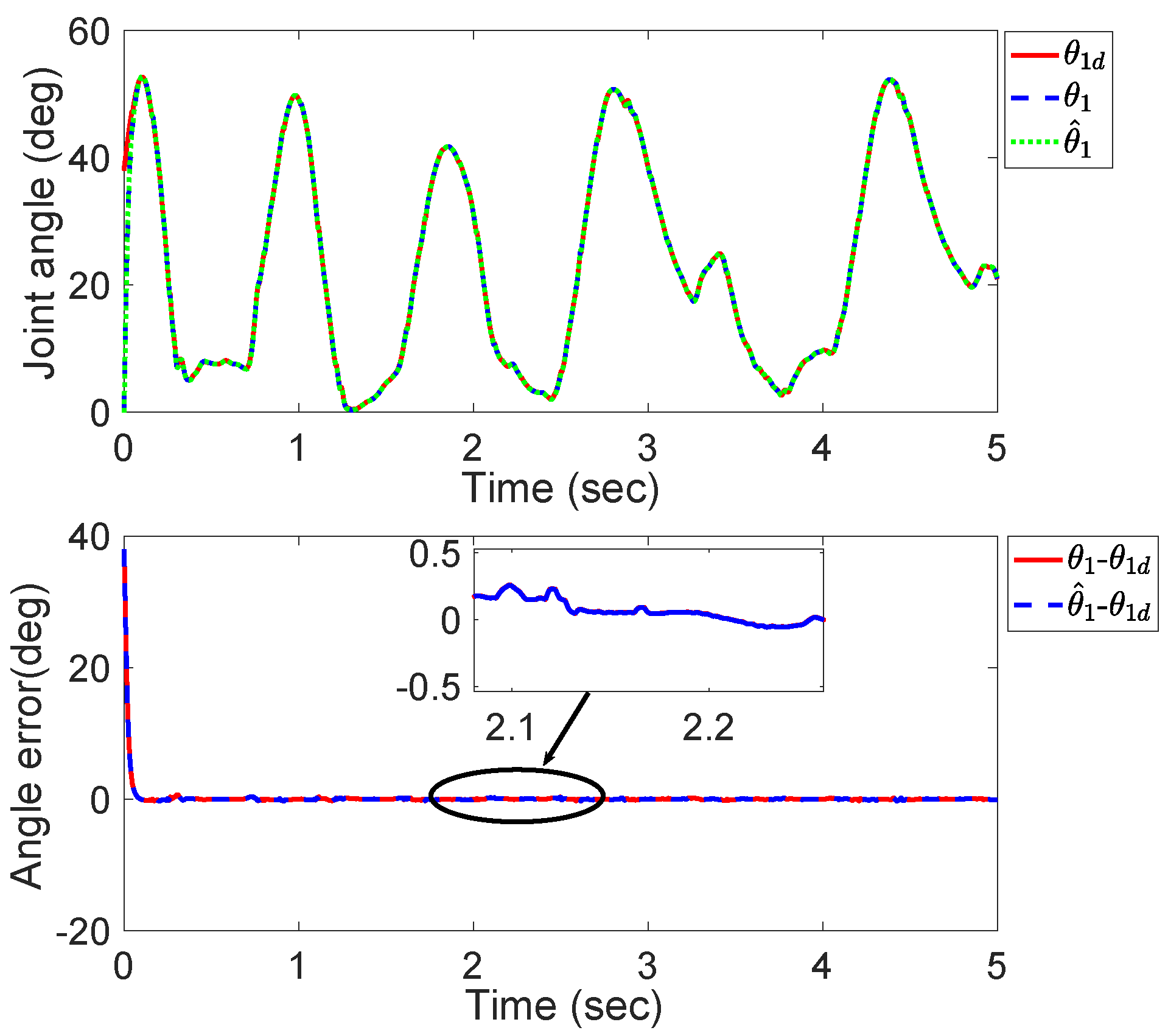
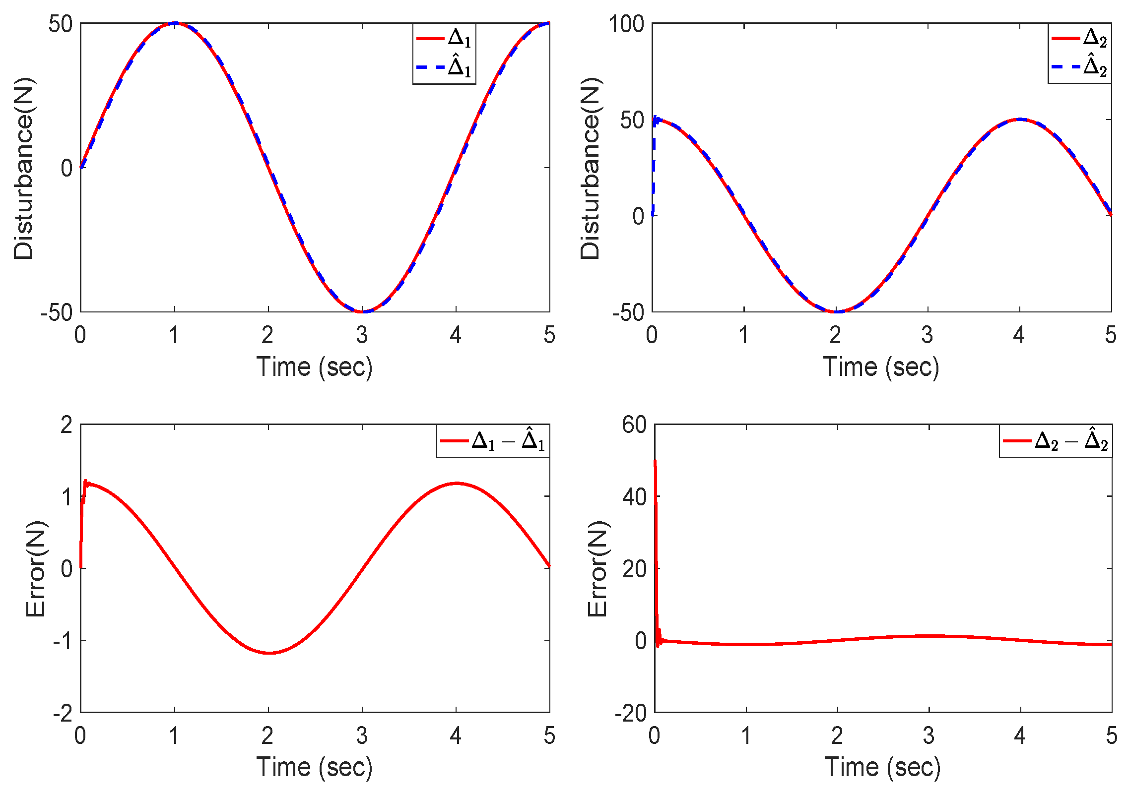
The passive control mode of human–exoskeleton cooperative motion is realized in this study, i.e., the exoskeleton joint angle $\theta ={[{\theta }_1,{\theta }_2]}^T$ tracks the input demands ${\theta }_d={[{\theta }_{d1},{\theta }_{d2}]}^T$ as shown in Figure 2. Hence, the tracking error is defined as $e=\theta -{\theta }_d$, and the sliding mode error is given by

$$s=\dot{e}+\sigma e,$$

(21)

where $\sigma \in {\mathbb{R}}^{2\times 2}$ is a positive diagonal matrix.

Then, the time derivative of s yields that

$$\begin{array}{c}\begin{array}{cc}\hfill \dot{s}& =\ddot{e}+\sigma \dot{e}\hfill \\ \hfill & =M_0^{-1}\left(\tau +{\tau }_{ext}-C_0{q}_2-G_0-{\tau }_{f,0}\right)\hfill \\ \hfill & -M_0^{-1}\Delta -{\ddot{\theta }}_d+\sigma \left(q_1-{\dot{\theta }}_d\right)\hfill \end{array}\end{array}.$$

(22)

The ideal sliding mode controller of exoskeleton is given by

$$\begin{array}{c}\begin{array}{cc}\hfill \tau & =-M_{0}Ks-{\tau }_{ext}+G_0+\phi \left(q\right)\hfill \\ \hfill & +\Delta +M_0{\ddot{\theta }}_d-M_0\sigma \left(q_1-{\dot{\theta }}_d\right)\hfill \end{array}\hfill \end{array},$$

(23)

where K is a positive control gain.

Since the lumped uncertainty $\Delta$ is unknown and the joint angular velocity $q_2$ is unmeasurable, the sliding mode controller is designed as

$$\begin{array}{c}\begin{array}{cc}\hfill \tau & =-M_{0}K\hat{s}-{\tau }_{ext}+G_0+\hat{\phi }\left(q\right)\hfill \\ \hfill & +M_0{\hat{q}}_3+M_0{\ddot{\theta }}_d-M_0\sigma \left(q_1-{\dot{\theta }}_d\right)\hfill \end{array}\hfill \end{array},$$

(24)

where $\hat{s}={\hat{q}}_2-{\dot{\theta }}_d+\sigma (q_1-{\theta }_d)$, $\hat{\phi }\left(q\right)=C_0{\hat{q}}_2+{\tau }_{f,0}$, ${\hat{q}}_2$ and ${\hat{q}}_3$ are obtained by the LESO (12).

Remark 2.

The lumped uncertainty Δ in (24) is compensated by regulating the sliding mode control gain and the observer bandwidth.

The Lyapunov function for the exoskeleton control is given by

$$V_t=s^{T}s/2+V_{\epsilon }.$$

(25)

Then, substituting $\dot{s}$ in (22), the time derivative of $V_t$ yields that

$$\begin{array}{c}\begin{array}{cc}\hfill {\dot{V}}_t& =s^T\dot{s}+{\dot{V}}_{\epsilon }\hfill \\ \hfill & =s^T{M}_0^{-1}\left(\tau +{\tau }_{ext}-\phi \left(q\right)-G_0\right)\hfill \\ \hfill & -s^T[M_0^{-1}\Delta +{\ddot{\theta }}_d-\alpha (q_1-{\dot{\theta }}_d)]+{\dot{V}}_{\epsilon }\hfill \end{array}\end{array}.$$

(26)

Meanwhile, substituting the sliding mode controller (24) into (26), we can see that

$$\begin{array}{c}\begin{array}{cc}\hfill {\dot{V}}_t& =-s^{T}Ks+s^{T}K\tilde{s}-s^T\left[M_0^{-1}\tilde{\phi }\left(q\right)-{\tilde{q}}_3-\sigma {\tilde{q}}_2\right]+{\dot{V}}_{\epsilon }\hfill \\ \hfill & \le -s^T\left(K-\frac{1}{2}I\right)s+\frac{1}{2}{\tilde{\Delta }}_d^T{\tilde{\Delta }}_d\hfill \\ \hfill & -\left(2{\omega }_0-\frac{2{\gamma }_1\alpha }{{\omega }_0}∥M_0^{-1}∥\right){∥\epsilon ∥}^2+\frac{2{\lambda }_2}{{\omega }_0^2}\left|\delta \left(t\right)\right|∥\epsilon ∥\hfill \end{array}\end{array},$$

(27)

where ${\tilde{\Delta }}_d=(K+\sigma ){\tilde{q}}_2-M_0^{-1}\tilde{\phi }\left(q\right)+{\tilde{q}}_3$ is the lumped estimation error.

In fact, the boundary of ${\tilde{\Delta }}_d^T{\tilde{\Delta }}_d$ is determined by the observer bandwidth ${\omega }_0$ in the designed LESO (12). Hence, the convergent speed of the sliding mode error s is decided by the control gain K and the observer bandwidth ${\omega }_0$. Furthermore, if s is converged into a zero neighborhood, the tracking error $e=\theta -{\theta }_d$ is also convergent.

Figure 2 shows the proposed sliding mode control scheme with the LESO. The exoskeleton dynamic model (7) involves the lumped uncertainty $\Delta$. Then, the linear extended state (12) is designed to address $\Delta$ and the unmeasured angular velocity $\dot{\theta }$. Meanwhile, the sliding mode controller (24) outputs the motor torque $\tau$ to guarantee the joint position tracking performance and to compensate the LESO estimation error.

5. Simulation

To verify the proposed sliding mode control scheme with the LESO, the corresponding nominal model functions are given by

$$\begin{array}{c}\begin{array}{cc}\hfill M_0\left(\theta \right)& =\left[\begin{array}{cc}25.7+3.2cos{\theta }_2& 6.9+1.6cos{\theta }_2\\ 6.9+1.6cos{\theta }_2& 6.9\end{array}\right]\hfill \\ \hfill C_0(\theta ,\dot{\theta })& =\left[\begin{array}{cc}-1.6{\dot{\theta }}_{2}sin{\theta }_2& -1.6sin{\theta }_2({\dot{\theta }}_1+{\dot{\theta }}_2)\\ 1.6{\dot{\theta }}_{1}sin{\theta }_2& 0\end{array}\right]\hfill \\ \hfill G_0\left(\theta \right)& =\left[\begin{array}{c}40.3sin({\theta }_1+{\theta }_2)+178.9sin{\theta }_1\\ 40.3sin({\theta }_1+{\theta }_2)\end{array}\right]\hfill \\ \hfill {\tau }_{f,0}\left(\dot{\theta }\right)& =\left[\begin{array}{c}27.8\mathrm{sgn}\left({\dot{\theta }}_1\right)+2.6{\dot{\theta }}_1\\ 37.2\mathrm{sgn}\left({\dot{\theta }}_2\right)+7.5{\dot{\theta }}_2\end{array}\right]\hfill \end{array}\hfill \end{array}.$$

(28)

Meanwhile, the lumped uncertainty is selected as $\Delta \left(t\right)={[50sin\left(0.5\pi t\right),50cos\left(0.5\pi t\right)]}^T$. The LESO bandwidth ${\omega }_0=200$ and the parameter and gain of sliding mode controller are $\sigma =\mathrm{diag}\{25,25\}$, $K=\mathrm{diag}\{100,100\}$.

The angle response of the exoskeleton’s two joints in the simulation are shown in Figure 3 and Figure 4. Both the tracking errors of the joint positions $|{\theta }_i-{\theta }_{id}|(i=1,2)$ and the estimation errors of the LESO $|{\theta }_i-{\hat{\theta }}_i(i=1,2)|$ are less than 0.5 deg, which indicates that the proposed controller has a favorable performance for the exoskeleton tracking the joint demands in the passive control mode of human–exoskeleton cooperative motion. Furthermore, the corresponding angle estimation ${\hat{\theta }}_i(i=1,2)$ also converges into the actual angle ${\theta }_i(i=1,2)$. Meanwhile, the lumped disturbance and the angular velocity estimations ${\hat{\Delta }}_i\{i=1,2\}$, ${\hat{\dot{\theta }}}_i\{i=1,2\}$ of two joints in the simulation are shown in Figure 5 and Figure 6. The corresponding estimation error is relatively small to guarantee that the LESO effectively existed in the controller design. The control torques of the two exoskeleton joints in the simulation are given in Figure 7.

It should be noted that, in the initial time, the control torques have a very large magnitude, since the initial tracking angle errors are obvious. Then, the control torques are reduced to small values with a little chatters due to the tiny tracking angle errors. The satisfactory estimation errors are guaranteed by the LESO to estimate these unknown disturbances together with some unmeasurable states. From the simulation results, the angular position and velocity estimations dynamically converge to the corresponding angle responses with high accuracy, which have verified the effectiveness of the proposed LESO. Certainly, the LESO estimation performance should be guaranteed to improve the stability and dynamic tracking performance of the designed controller. The proposed controller can guarantee that the exoskeleton joint angles track general demand input with a certain frequency. Some angle demands with a high frequency cannot be well tracked due to the limited performance of the exoskeleton-driving element of the servo motor actuator.

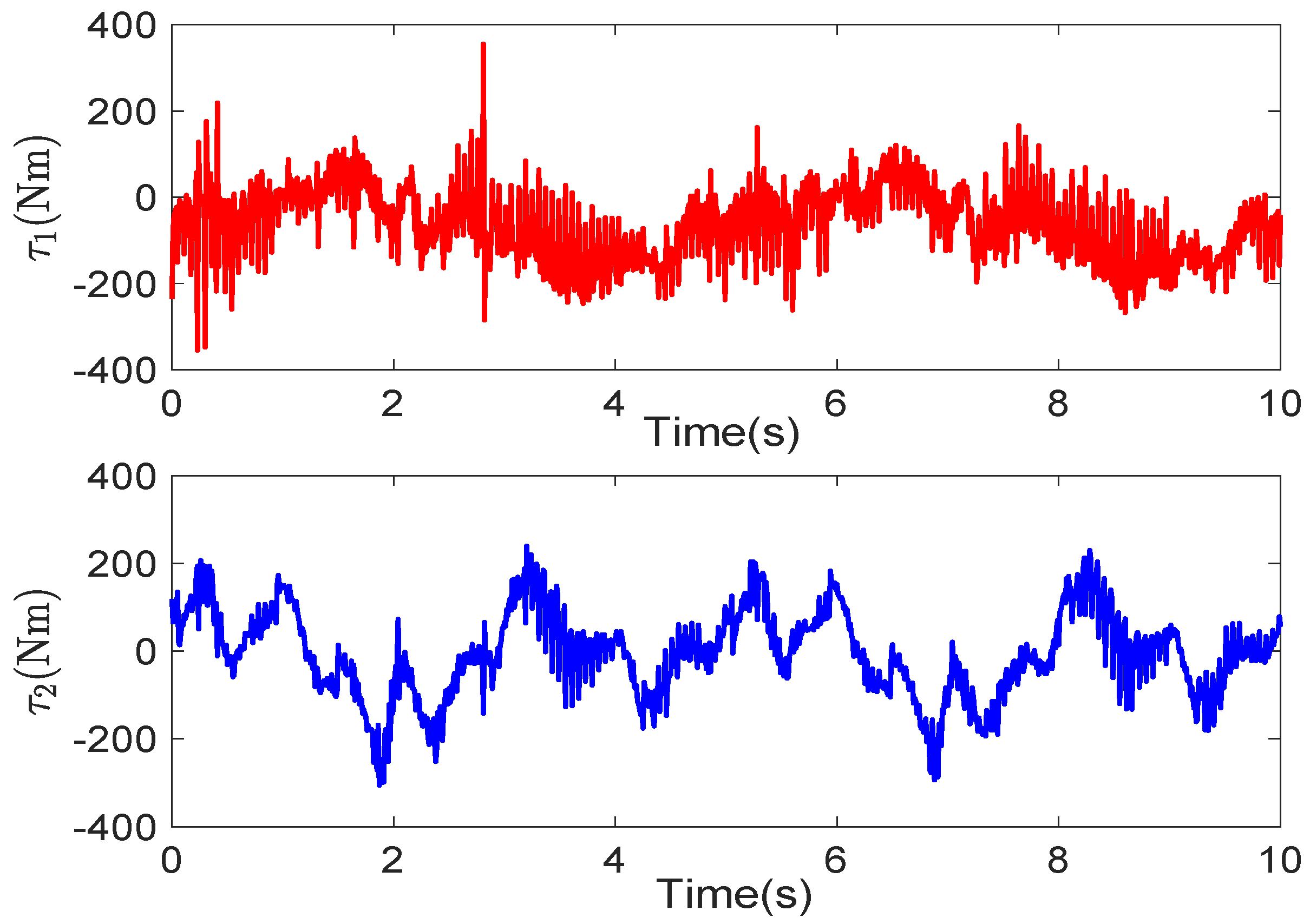
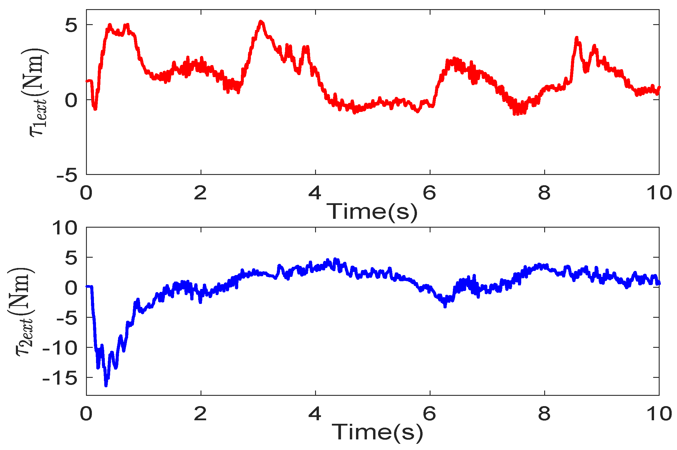
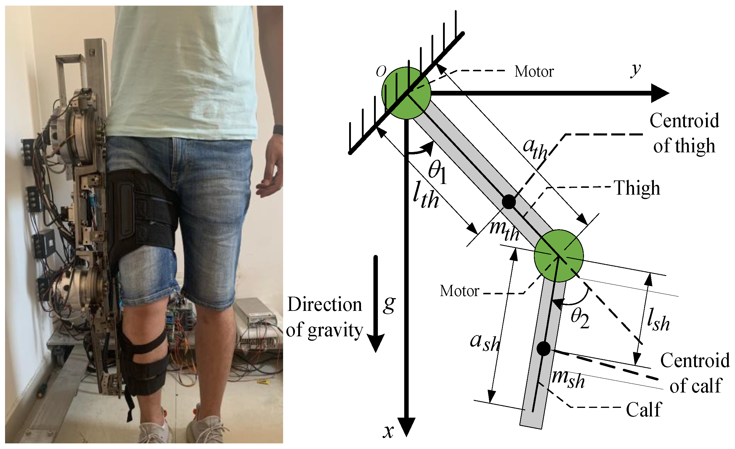
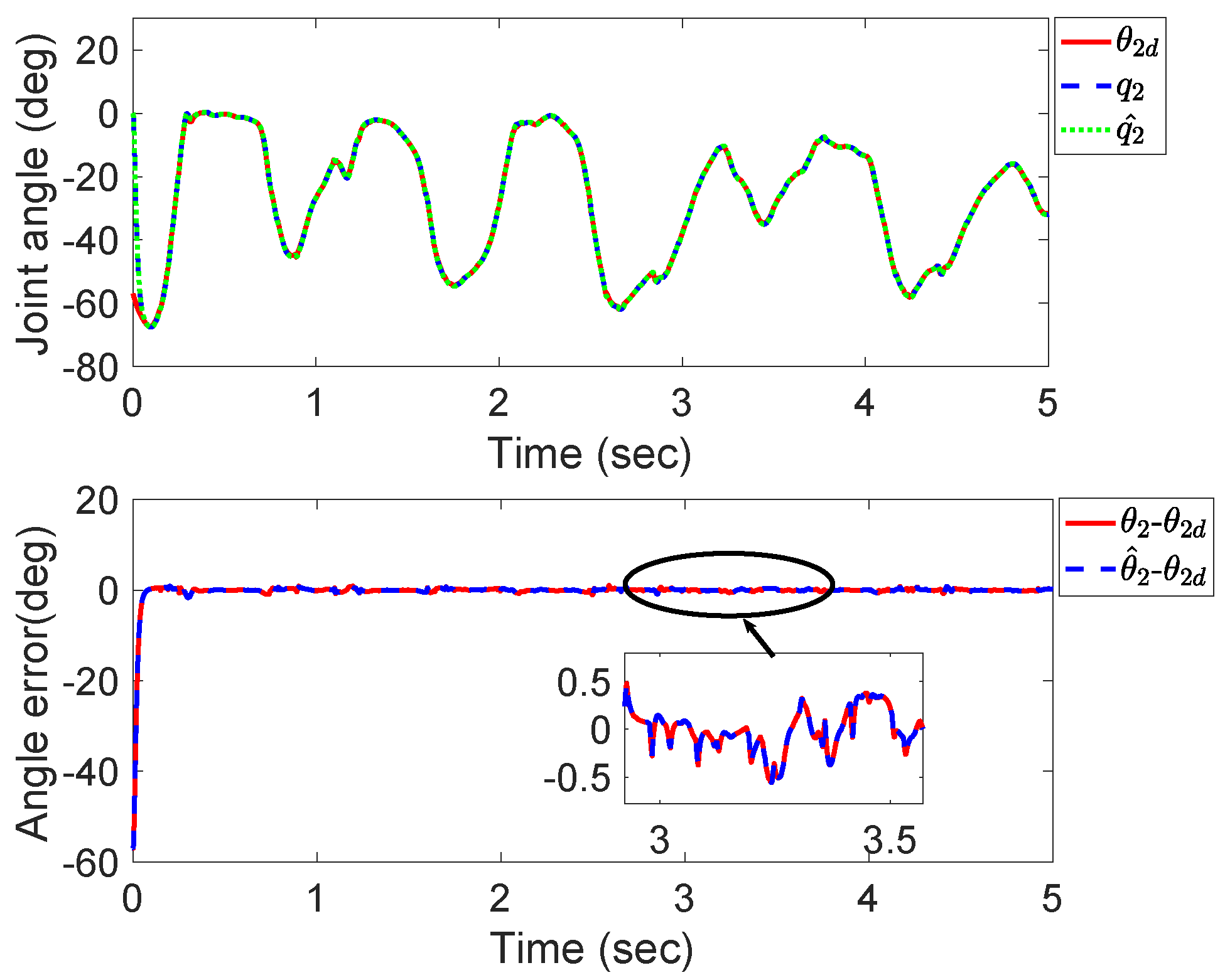
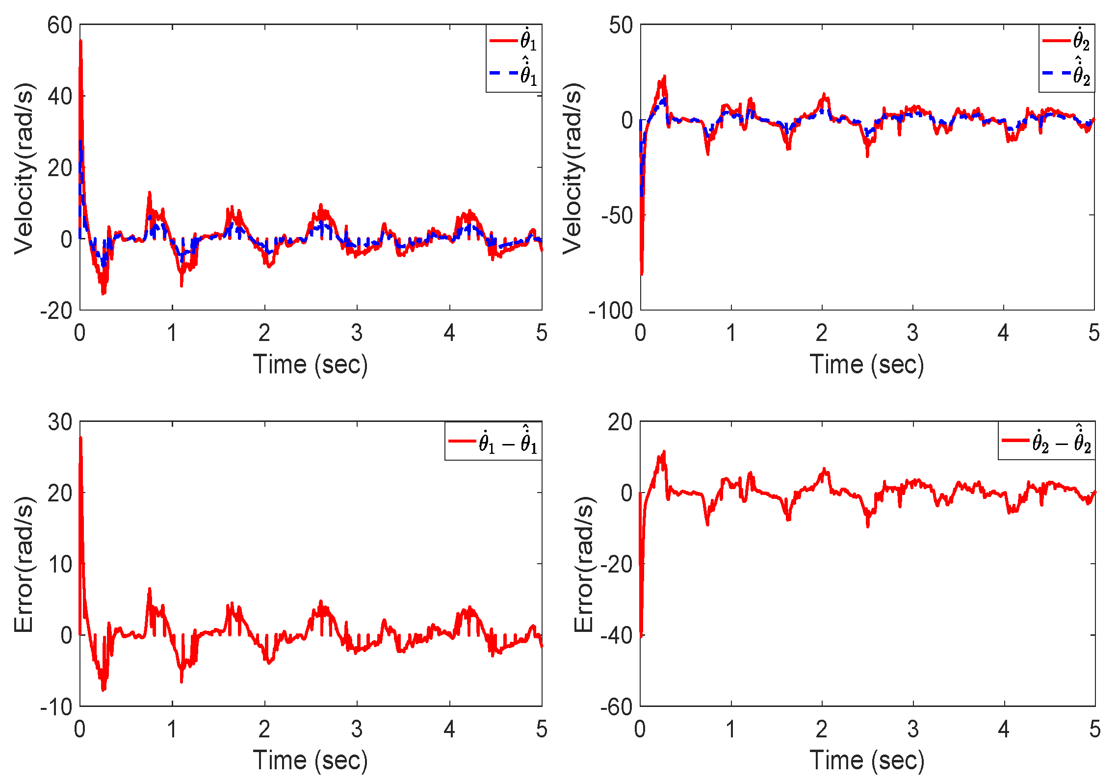
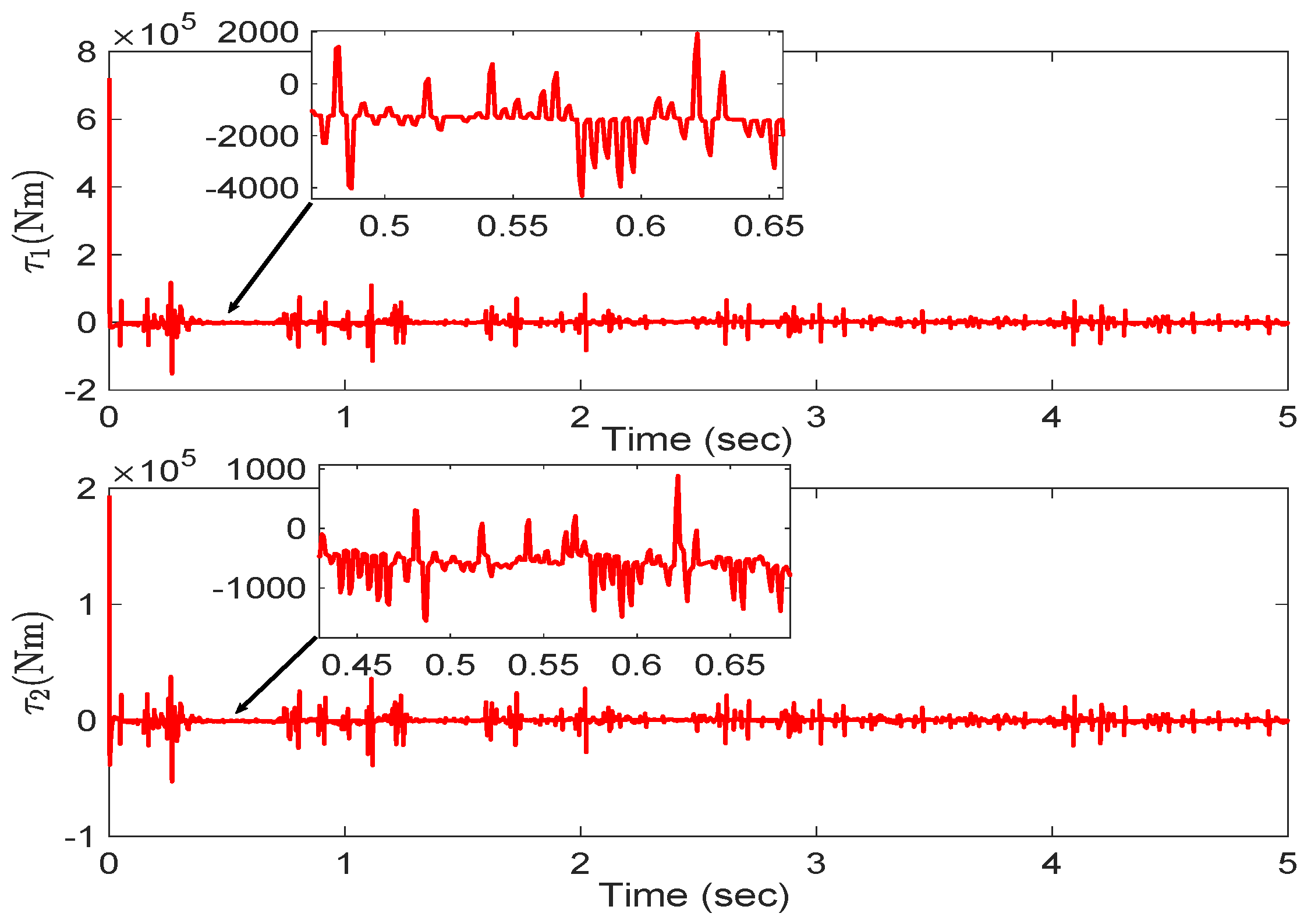
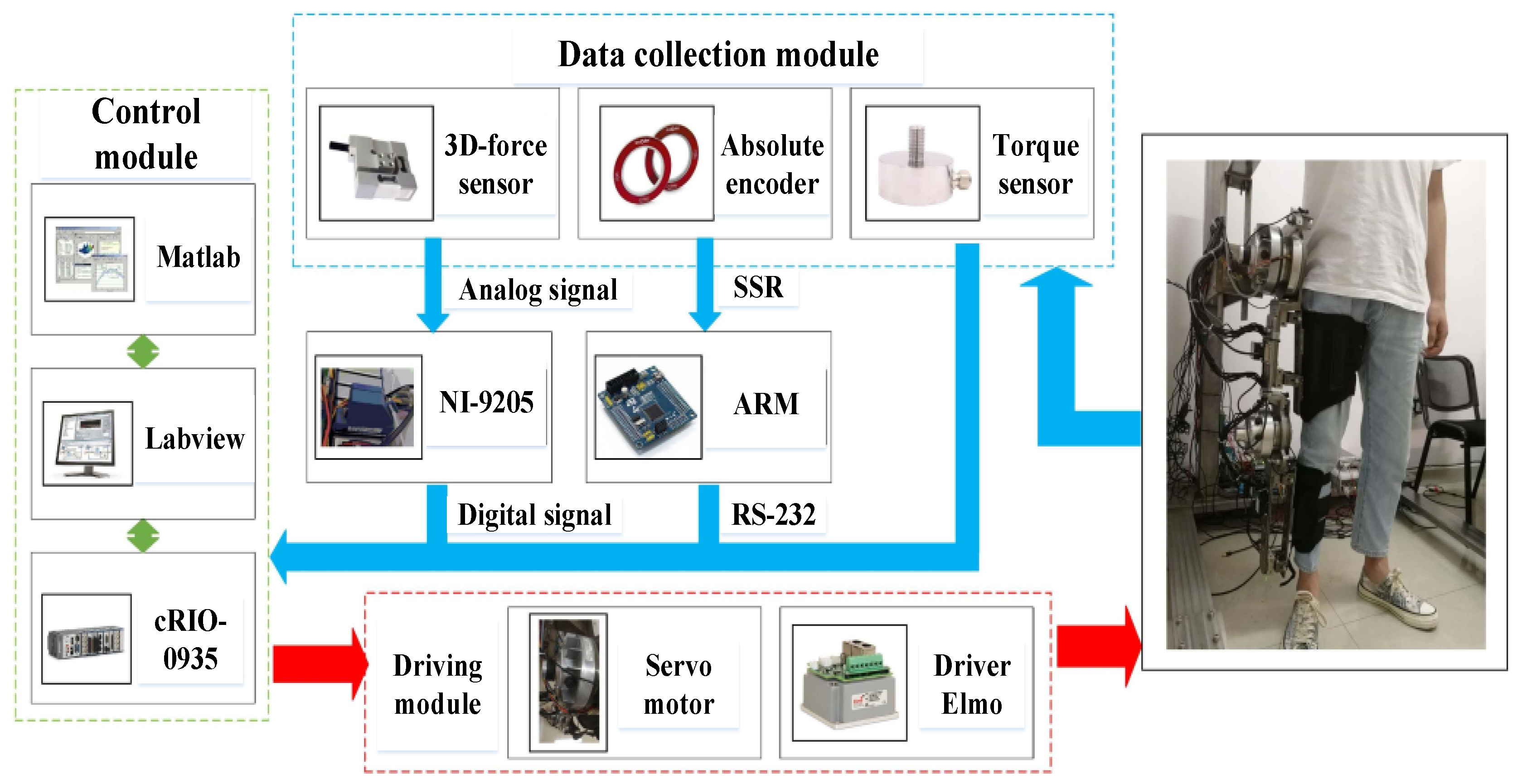
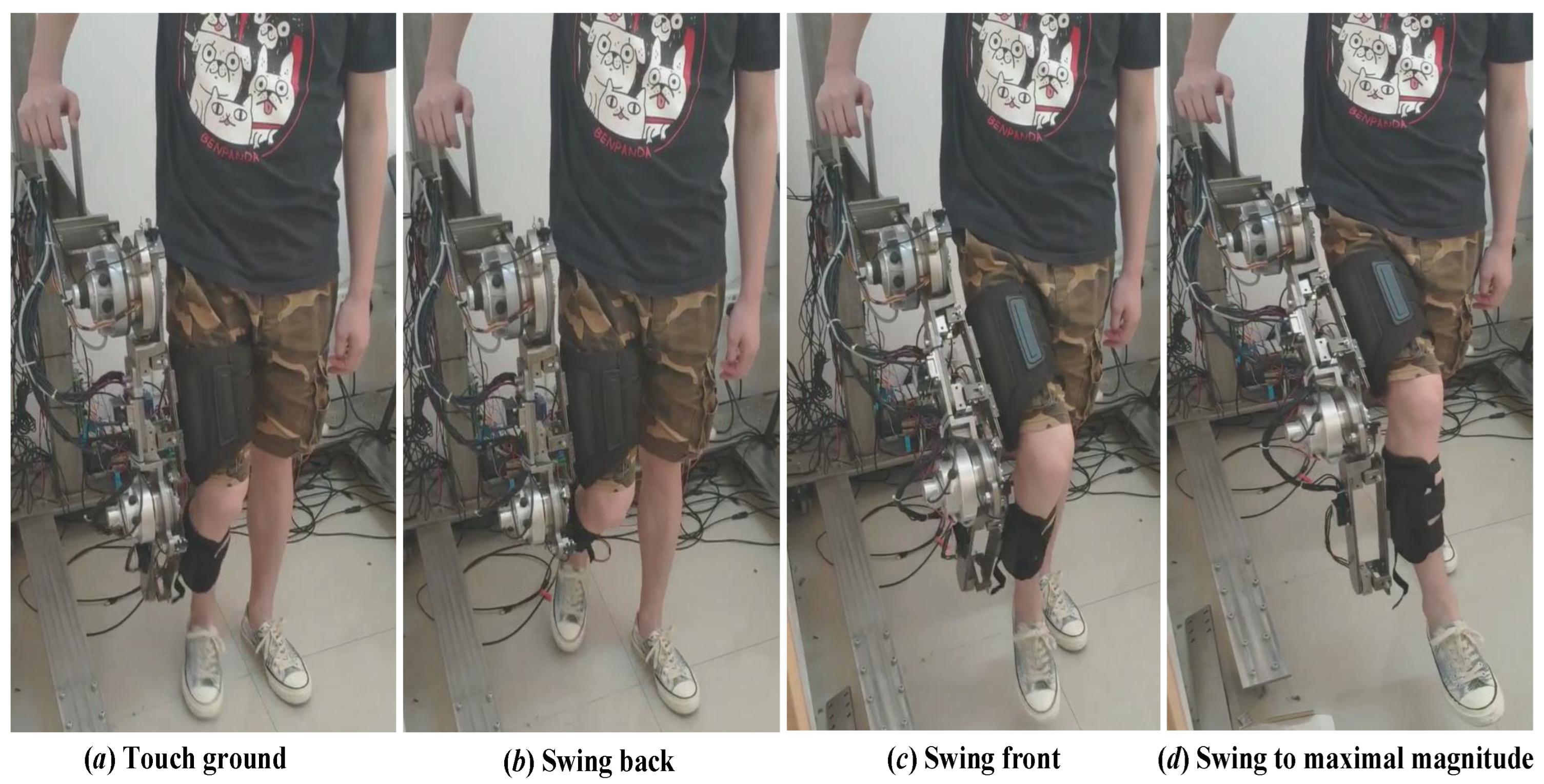
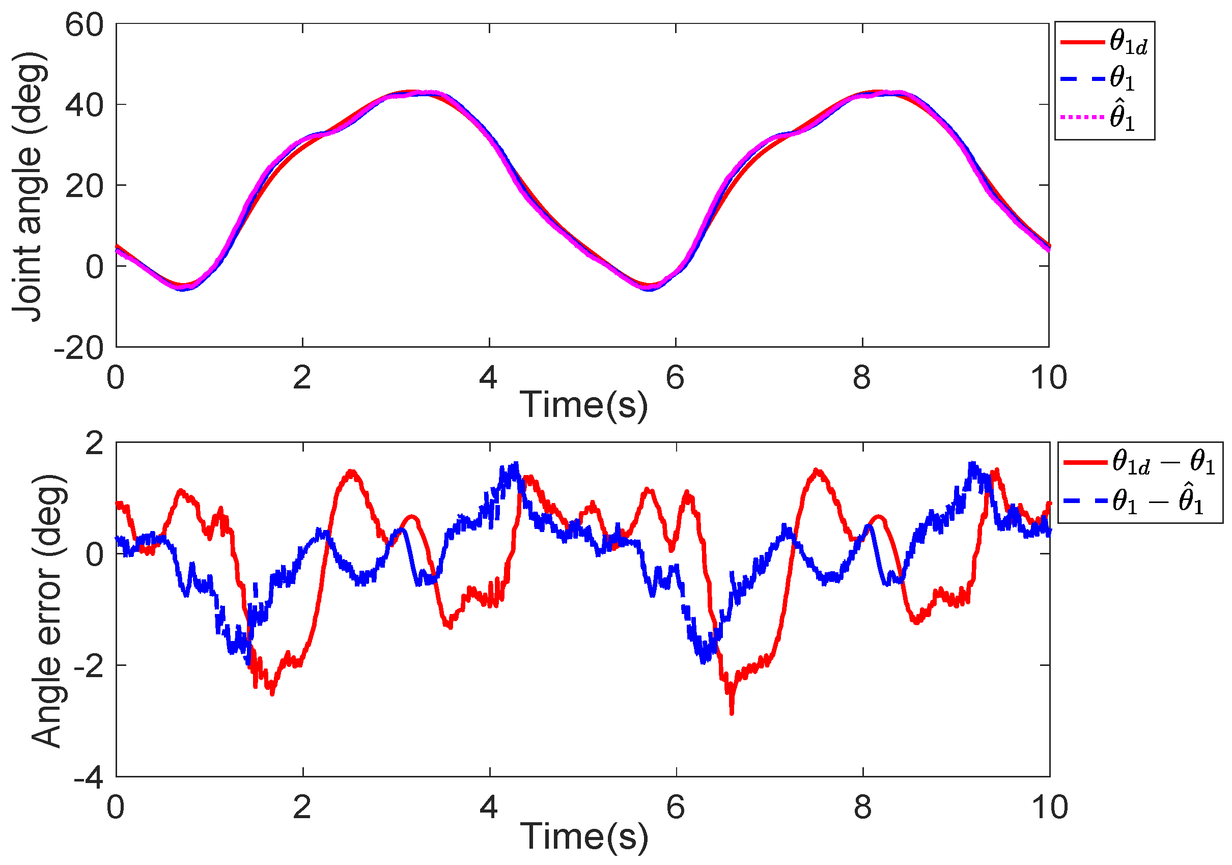
6. Experiment Verification

The proposed controller is also verified by the experiment. Firstly, the 2-DOF lower limb exoskeleton platform is constructed as shown in Figure 8. The LESO bandwidth parameter and gains of the sliding mode controller are the same as in the simulation. The whole weight of the exoskeleton platform is about 20 kg, excluding the fixed bracket. The driven power is the ordinary AC with 50 Hz rather than a lithium battery, to guarantee the long duration of the experiment. The actuators are two servo motors (GDM1-100N2/120N2), which are driven by the driver (Elmo-G-SOLHOR15/100EE). Meanwhile, the joint positions and the human–exoskeleton interaction torques are measured by absolute encoders (INC-4-150/3-125) and 3-D force sensors (JNSH-2-10kg-BSQ-12). The controller (NI cRIO-9035) is realized in the Labview environment.

Table 2. The experimental component brand of the 2-DOF lower limb exoskeleton.

Component	Brand	Number
Servo motor	GDM1-100N2/120N2	2
Motor driver	Elmo-G-SOLHOR15/100EE	2
Absolute encoders	INC-4-150/3-125	2
3-D force sensors	JNSH-2-10kg-BSQ-12	4
Controller	NI cRIO-9035	1

lists the respective experimental component brand of the 2-DOF lower limb exoskeleton. The proposed control algorithm is programmed by Matlab/Simulink to generate a .os file, which is downloaded into the Labview software and runs in the hardware controller. In this experiment, the passive control model of the exoskeleton is realized by one operator wearing the exoskeleton. Then, the exoskeleton is controlled to track the prescribed demand input. The operator tolerates the human–exoskeleton impedance as the human–exoskeleton cooperative motion is periodically carried out. The calculated interval of the proposed control algorithm is 10 ms, which means that the sensor information sampling, data communication, and algorithm computation are carried out in 10 ms intervals. The stability and performance of this control algorithm are feasible for guaranteeing the satisfactory synchronous effect of the human–exoskeleton cooperative motion.

The experimental scene of the exoskeleton motion control is shown in Figure 9. The exoskeleton has four obvious gait phases: touch ground, swing back, swing front, and swing to maximal magnitude. These four gait phases perform periodic replacement of one another. As these four gait phases finish, the whole walking gait is realized in one duration. Of course, different operators have disparate walking gaits with different motion magnitudes. However, the maximal motion magnitude is finite, which is constrained within a reasonable range of human motion gait.

By using the LESO, the experimental hip tracking error $|{\theta }_1-{\theta }_{1d}| < 2$ deg, while the knee tracking error $|{\theta }_2-{\theta }_{2d}| < 5$ deg is shown in Figure 10 and Figure 11, which are a satisfactory performance for a human–exoskeleton cooperative motion experiment. Furthermore, the joint estimation errors $|{\theta }_i-{\hat{\theta }}_i|$ are less than the corresponding tracking error $|{\theta }_i-{\theta }_{id}|$. This phenomenon is also reasonable, since the LESO is a similar inner-loop of the whole SMC control loop of the exoskeleton. In other words, the inner-loop state estimation error should be less than the outer-loop position tracking error. Hence, the experimental results are consistent with the simulation, with a satisfactory tracking performance of the proposed sliding mode controller. The tracking accuracy of the hip angle response is better than that of the knee joint, since the peak torque performance of the hip motor is larger than that of the knee motor.

In addition, the motor torques of the two joints ${\tau }_i(i=1,2)$ are given in Figure 12. The maximal motor torque is less than 400 Nm, which is constrained by the maximal power of the servo motor. If the external load of the exoskeleton increases, the motor torque will exceed the maximal power limitation, which leads to the motor system crashes.

Finally, the human–exoskeleton interaction torques of the two joints are given in Figure 13, and have less than 5 Nm in the steady state response for the proposed sliding mode controller. In fact, these interaction torques are called human–exoskeleton impedance, which evaluates the wearable performance of the operator, since the operator must overcome the impedance by his muscle energy. It is tolerated by the operator in the human–exoskeleton cooperative motion. If the interaction torques obviously increase, the wearable comfort of the operator will decline in long term motion.

7. Discussion

Different from many admittance controllers used in the exoskeleton, the proposed sliding mode controller is a typical passive control scheme for human–exoskeleton cooperative motion. This control scheme also guarantees high joint position tracking accuracy to realize the operator synchronized to the exoskeleton. Furthermore, the human–exoskeleton interaction torque is tolerable for the operator in the experiment. The admittance control scheme also guarantees a very small human–exoskeleton interaction torque by using an admittance model design. However, the joint position tracking performance may simultaneously not be ensured.

8. Conclusions

In this study, a sliding mode controller based on a linear extended state observer (LESO) is proposed for a 2-DOF lower limb exoskeleton to improve the tracking performance of the passive control mode in human–exoskeleton cooperative motion. The LESO is used to estimate the unmeasurable angular velocity and the uncertainties in the Lagrangian model. Then, the sliding mode controller is designed to guarantee that the joint tracking error converges to a small-enough zero neighborhood. Finally, both simulation and experimental results indicate that the proposed control scheme has a satisfactory performance for the exoskeleton in terms of tracking the joint demands with high accuracy. However, the human–exoskeleton interaction torques cannot guarantee a further reduction in this study. In future work, we will consider two-motion mode fusion between the admittance control and the model-based control with respect to various walking frequencies in human–exoskeleton cooperative motion. We will also try to find the potential advantages of two-motion control modes in a complex human–exoskeleton interaction environment.

References

1. Collins, S.H.; Wiggin, M.B.; Sawicki, G.S. Reducing the energy cost of human walking using an unpowered exoskeleton. Nature 2015, 522, 212–215. [Google Scholar] [CrossRef]
2. Gregorczyk, K.N.; Hasselquist, L.; Schiffman, J.M.; Bensel, C.K.; Obusek, J.P.; Gutekunst, D.J. Effects of a lower-body exoskeleton device on metabolic cost and gait biomechanics during load carriage. Ergonomics 2010, 53, 1263–1275. [Google Scholar] [CrossRef]
3. Kawamoto, H.; Sankai, Y. Power assist method based on Phase Sequence and muscle force condition for HAL. Adv. Robot. 2005, 19, 717–734. [Google Scholar] [CrossRef]
4. Lee, J.W.; Kim, H.; Jang, J.; Park, S. Virtual model control of lower extremity exoskeleton for load carriage inspired by human behavior. Autonom. Robot. 2015, 38, 211–223. [Google Scholar] [CrossRef]
5. Zoss, A.; Kazerooni, H. Design of an electrically actuated lower extremity exoskeleton. Adv. Robot. 2006, 20, 967–988. [Google Scholar] [CrossRef]
6. Shields, B.; Goldfarb, M. Design and Energetic Characterization of a Solenoid Injected Liquid Monopropellant Powered Actuator for Self-Powered Robots. In Proceedings of the 2005 IEEE-ICRA, Barcelona, Spain, 18–22 April 2005. [Google Scholar]
7. Lu, R.; Li, Z.; Su, C.Y.; Xue, A. Development and Learning Control of a Human Limb With a Rehabilitation Exoskeleton. IEEE Trans. Ind. Electron. 2014, 61, 3776–3785. [Google Scholar] [CrossRef]
8. Chen, Z.; Guo, Q.; Li, T.; Yan, Y.; Jiang, D. Gait prediction and variable admittance control for lower limb exoskeleton with measurement delay and extended-state-observer. IEEE Trans. Neural Netw. Learn. Syst. 2022. [Google Scholar] [CrossRef]
9. Chen, Z.; Guo, Q.; Li, T.; Yan, Y. Output constrained control of lower limb exoskeleton based on knee motion probabilistic model with finite-time extended state observer. IEEE/ASME Trans. Mechatron. 2023, 28, 2305–2316. [Google Scholar] [CrossRef]
10. Yang, Y.; Ma, L.; Huang, D. Development and repetitive learning control of lower limb exoskeleton driven by electro-hydraulic actuators. IEEE Trans. Ind. Electron. 2017, 64, 4169–4178. [Google Scholar] [CrossRef]
11. Guo, Q.; Zhang, Y.; Jiang, D. A control approach for human-mechatronic-hydraulic-coupled exoskeleton in overload-carrying condition. Int. J. Robot. Autom. 2016, 31, 272–280. [Google Scholar]
12. Li, Z.; Su, C.; Li, G.; Hang, S. Fuzzy approximation-based adaptive backstepping control of an exoskeleton for human upper limbs. IEEE Trans. Fuzzy Syst. 2014, 23, 555–566. [Google Scholar] [CrossRef]
13. Li, Z.; Su, C.Y.; Wang, L.; Chen, Z.; Chai, T. Nonlinear disturbance observer-based control design for a robotic exoskeleton incorporating fuzzy approximation. IEEE Trans. Ind. Electron. 2015, 62, 5763–5775. [Google Scholar] [CrossRef]
14. He, W.; Li, Z.; Dong, Y.; Zhao, T. Design and adaptive control for an upper limb robotic exoskeleton in presence of input saturation. IEEE Trans. Neural Netw. Learn. Syst. 2018, 30, 97–108. [Google Scholar] [CrossRef]
15. Han, S.; Wang, H.; Tian, Y. A linear discrete-time extended state observer-based intelligent PD controller for a 12 DOFs lower limb exoskeleton LLE-RePA. Mech. Syst. Signal Proc. 2020, 138, 106547. [Google Scholar] [CrossRef]
16. Meng, W.; Liu, Q.; Zhou, Z.; Ai, Q.; Sheng, B.; Xie, S.S. Recent development of mechanisms and control strategies for robot-assisted lower limb rehabilitation. Mechatronics 2015, 31, 132–145. [Google Scholar] [CrossRef]
17. Hussain, S.; Xie, S.Q.; Jamwal, P.K. Robust nonlinear control of an intrinsically compliant robotic gait training orthosis. IEEE Trans. Syst. Man Cybern. Syst. 2012, 43, 655–665. [Google Scholar] [CrossRef]
18. Saglia, J.A.; Tsagarakis, N.G.; Dai, J.S.; Caldwell, D.G. Control strategies for patient-assisted training using the ankle rehabilitation robot (ARBOT). IEEE/ASME Trans. Mechatron. 2012, 18, 1799–1808. [Google Scholar] [CrossRef]
19. Chen, Z.; Guo, Q.; Yan, Y.; Shi, Y. Model identification and adaptive control of lower limb exoskeleton based on neighborhood field optimization. Mechatronics 2022, 81, 102699. [Google Scholar] [CrossRef]
20. Chen, Z.; Guo, Q.; Li, T.; Shi, Y. Distributed adaptive impedance control of networked Lagrangian systems with neighborhood interaction feedback. Int. J. Robust Nonlin. 2022, 32, 2251–2272. [Google Scholar] [CrossRef]
21. Keemink, A.Q.; van der Kooij, H.; Stienen, A.H. Admittance control for physical human-robot interaction. Int. J. Robot. Res. 2018, 37, 1421–1444. [Google Scholar] [CrossRef]
22. Li, Z.; Huang, B.; Ye, Z.; Deng, M.; Yang, C. Physical human-robot interaction of a robotic exoskeleton by admittance control. IEEE Trans. Ind. Electron. 2018, 65, 9614–9624. [Google Scholar] [CrossRef]
23. Yu, X.; He, W.; Li, Y.; Xue, C.; Li, J.; Zou, J.; Yang, C. Bayesian estimation of human impedance and motion intention for human-robot collaboration. IEEE Trans. Cybern. 2019, 51, 1822–1834. [Google Scholar] [CrossRef]
24. Guo, Q.; Chen, Z. Neural adaptive control of single-rod electrohydraulic system with lumped uncertainty. Mech. Syst. Signal Proc. 2021, 146, 106869. [Google Scholar] [CrossRef]
25. Guo, Q.; Zhang, Y.; Celler, B.G.; Su, S.W. Neural adaptive backstepping control of a robotic manipulator with prescribed performance constraint. IEEE Trans. Neural Netw. Learn. Syst. 2018, 30, 3572–3583. [Google Scholar] [CrossRef]
26. Binh, N.T.; Tung, N.A.; Nam, D.P.; Quang, N.H. An adaptive backstepping trajectory tracking control of a tractor trailer wheeled mobile robot. Int. J. Control Autom. Syst. 2019, 17, 465–473. [Google Scholar] [CrossRef]
27. Liu, J.; Gai, W.; Zhang, J.; Li, Y. Nonlinear adaptive backstepping with ESO for the quadrotor trajectory tracking control in the multiple disturbances. Int. J. Control Autom. Syst. 2019, 17, 2754–2768. [Google Scholar] [CrossRef]
28. He, W.; Meng, T.; Huang, D.; Li, X. Adaptive boundary iterative learning control for an Euler-Bernoulli beam system with input constraint. IEEE Trans. Neural Netw. Learn. Syst. 2018, 29, 1539–1549. [Google Scholar] [CrossRef]
29. Li, Z.; Zhao, K.; Zhang, L.; Wu, X.; Zhang, T.; Li, Q.; Li, X.; Su, C.Y. Human-in-the-loop control of a wearable lower limb exoskeleton for stable dynamic walking. IEEE/ASME Trans. Mechatron. 2021, 26, 2700–2711. [Google Scholar] [CrossRef]
30. Sun, W.; Lin, J.W.; Su, S.F.; Wang, N.; Er, M.J. Reduced adaptive fuzzy decoupling control for lower limb exoskeleton. IEEE Trans. Cybern. 2020, 51, 1099–1109. [Google Scholar] [CrossRef]
31. Han, J.; Yang, S.; Xia, L.; Chen, Y.H. Deterministic adaptive robust control with a novel optimal gain design approach for a fuzzy 2-DOF lower limb exoskeleton robot system. IEEE Trans. Fuzzy Syst. 2020, 29, 2373–2387. [Google Scholar] [CrossRef]
32. Yang, Y.; Li, Y.; Liu, X.; Huang, D. Adaptive neural network control for a hydraulic knee exoskeleton with valve deadband and output constraint based on nonlinear disturbance observer. Neurocomputing 2022, 473, 14–23. [Google Scholar] [CrossRef]
33. Zhang, G.; Wang, J.; Yang, P.; Guo, S. Iterative learning sliding mode control for output-constrained upper-limb exoskeleton with non-repetitive tasks. Appl. Math. Model. 2021, 97, 366–380. [Google Scholar] [CrossRef]
34. Liu, Y.; Fu, Y.; He, W.; Hui, Q. Modeling and observer-based vibration control of a flexible spacecraft with external disturbances. IEEE Trans. Ind. Electron. 2018, 66, 8648–8658. [Google Scholar] [CrossRef]
35. Nie, J.; Wang, H.; Lu, X.; Lin, X.; Sheng, C.; Zhang, Z.; Song, S. Finite-time output feedback path following control of underactuated MSV based on FTESO. Ocean Eng. 2021, 224, 108660. [Google Scholar] [CrossRef]
36. Ali, N.; Tawiah, I.; Zhang, W. Finite-time extended state observer based nonsingular fast terminal sliding mode control of autonomous underwater vehicles. Ocean Eng. 2020, 218, 108179. [Google Scholar] [CrossRef]
37. Tuo, Y.; Wang, S.; Guo, C. Finite-time extended state observer-based area keeping and heading control for turret-moored vessels with uncertainties and unavailable velocities. Int. J. Nav. Archit. Ocean Eng. 2022, 14, 100422. [Google Scholar] [CrossRef]
38. Wu, Q.; Chen, Y. Adaptive cooperative control of a soft elbow rehabilitation exoskeleton based on improved joint torque estimation. Mech. Syst. Signal Proc. 2023, 184, 109748. [Google Scholar] [CrossRef]
39. Wu, Q.; Wang, X.; Chen, B.; Wu, H. Development of a minimal-intervention-based admittance control strategy for upper extremity rehabilitation exoskeleton. IEEE Trans. Syst. Man Cybern. Syst. 2018, 48, 1005–1016. [Google Scholar] [CrossRef]
40. Guo, Q.; Zhang, Y.; Celler, B.G.; Su, S.W. Backstepping control of electro-hydraulic system based on extended-state-observer with plant dynamics largely unknown. IEEE Trans. Ind. Electron. 2016, 63, 6909–6920. [Google Scholar] [CrossRef]
41. Cui, R.; Chen, L.; Yang, C.; Chen, M. Extended state observer-based integral sliding mode control for an underwater robot with unknown disturbances and uncertain nonlinearities. IEEE Trans. Ind. Electron. 2017, 64, 6785–6795. [Google Scholar] [CrossRef]
42. Chen, Z.; Guo, Q.; Xiong, H.; Jiang, D.; Yan, Y. Control and implementation of 2-DOF lower limb exoskeleton experiment platform. Chin. J. Mech. Eng. 2021, 34, 22. [Google Scholar] [CrossRef]
43. Chen, Z.; Guo, Q.; Jiang, D.; Yan, Y. Robust sliding mode control for a 2-DOF lower limb exoskeleton base on linear extended state observer. Mech. Eng. Sci. 2020, 2, 1–6. [Google Scholar] [CrossRef]
44. Nadhynee, M.F.; Luis, A.C.; Agustin, U.; Alberto, L.J.; Isaac, C. Robust disturbance rejection control of a biped robotic system using high-order extended state observer. ISA Trans. 2016, 62, 276–286. [Google Scholar]
45. Fareh, R.; Khadraoui, S.; Abdallah, M.Y.; Baziyad, M.; Bettayeb, M. Active disturbance rejection control for robotic systems: A review. Mechatronics 2021, 80, 102671. [Google Scholar] [CrossRef]
46. Siciliano, B.; Sciavicco, L.; Villani, L.; Oriolo, G. Robotics: Modelling, Planning and Control; Springer Science & Business Media: Berlin/Heidelberg, Germany, 2010. [Google Scholar]
47. Zheng, Q.; Gao, L.Q.; Gao, Z. On stability analysis of active disturbance rejection control for nonlinear time-varying plants with unknown dynamics. In Proceedings of the 46th IEEE Conference on Decision and Control, DEC 2007, New Orleans, LA, USA, 12–14 December 2007; pp. 4090–4095. [Google Scholar]
Figure 1. The 2-DOF lower limb exoskeleton.
Actuators 12 00402 g001
Figure 2. The sliding mode control scheme with the LESO.
Actuators 12 00402 g002
Figure 3. The hip angle response of simulation ( θ 1 d : the angle demand, θ 1 : the angle response of exoskeleton, θ ^ 1 : the angle estimation of the LESO).
Actuators 12 00402 g003
Figure 4. The knee angle response of simulation ( θ 2 d : the angle demand, q 2 = θ 2 : the angle response of exoskeleton, q ^ 2 = θ ^ 2 : the angle estimation of the LESO).
Actuators 12 00402 g004
Figure 5. The lumped disturbance estimation of two joints in simulation ( Δ i { i = 1 , 2 } : the lumped disturbance of hip and knee, Δ ^ i { i = 1 , 2 } : the disturbance estimation of the LESO).
Actuators 12 00402 g005
Figure 6. The angular velocity estimation of two joints in simulation ( θ ˙ i { i = 1 , 2 } : the angular velocity of hip and knee, θ ˙ ^ i { i = 1 , 2 } : the angular velocity estimation of the LESO).
Actuators 12 00402 g006
Figure 7. The control torque of two joints in simulation ( τ 1 : the hip control torque, τ 2 : the knee control torque).
Actuators 12 00402 g007
Figure 8. The 2-DOF lower limb exoskeleton platform, and the color arrows represent the signal transmission between two modules.
Actuators 12 00402 g008
Figure 9. The experimental scene of the exoskeleton motion control.
Actuators 12 00402 g009
Figure 10. The hip angle response of experiment ( θ 1 d : the angle demand, θ 1 : the angle response of exoskeleton, θ ^ 1 : the angle estimation of the LESO).
Actuators 12 00402 g010
Figure 11. The knee angle response of experiment ( θ 2 d : the angle demand, θ 2 : the angle response of exoskeleton, θ ^ 1 : the angle estimation of the LESO).
Actuators 12 00402 g011
Figure 12. The motor torque of two joints in the experiment ( τ 1 : the hip motor torque, τ 2 : the knee motor torque).
Actuators 12 00402 g012
Figure 13. The human–exoskeleton interaction torques of two joints ( τ 1 e x t : the human–exoskeleton interaction torque of hip joint, τ 2 e x t : the human–exoskeleton interaction torque of knee joint).
Actuators 12 00402 g013