A Survey on Autonomous Offline Path Generation for Robot-Assisted Spraying Applications

Abstract

Robot-assisted spraying is a widespread manufacturing process for coating a multitude of mechanical components in an efficient and cost-effective way. However, process preparation is very time-consuming and relies heavily on the expertise of the robot programmer for generating the appropriate robot trajectory. For this reason, industry and academia investigate the possibility of supporting the end-user in the process by the use of appropriate algorithms. Mostly partial concepts can be found in the literature instead of a solution that solves this task end-to-end. This survey paper provides a summary of previous research in this field, listing the frameworks developed with the intention of fully automating the coating processes. First, the main inputs required for the trajectory calculation are described. The path-generating algorithm and its subprocesses are then classified and compared with alternative approaches. Finally, the required information for the executable output program is described, as well as the validation tools to keep track of program performance. The paper comes to the conclusion that there is a demand for an autonomous robot-assisted spraying system, and with a call-for-action for the implementation of the holistic framework.

1. Introduction

Spraying processes are surface treatment techniques that allow mechanical components to be coated with additional layers of coating material. The general procedure includes having a spray gun pass over the entire surface of a component while emitting the specified material. When the surface is covered, this material solidifies, thus generating an additional layer. Two widespread spraying-based technologies are chemical coating and thermal spraying [1]. Typical applications of this surface technology are aesthetic modifications (e.g., changing the surface’s color), improving the functionality and performance of the part (e.g., thermal barrier, biocompatibility, adhesion, or electrical conductivity), and improving the component life expectancy (e.g., protection against wear, abrasion, erosion, corrosion, or oxidation) [2].

A widespread technical solution to improve the efficiency of the spraying process is the use of industrial robots [3]. The main reasons for using these are, first, the fact that the quality of the process is ensured by the high repeatability of the automated process; second, the fact that the safety of human operators is guaranteed by restricting their exposure to high temperatures, vapors, and fumes emitted in the process; and third, that there is an economic benefit in increasing the throughput of processed components since a robot is capable of working at a higher speed and for longer periods of time than a human operator.

Despite all the benefits that robots bring to these manufacturing tasks, there are several hurdles that prevent the adoption of automated spraying. The process of programming a robot for this type of application is still fairly manual [4]. This applies not only to spraying processes but also to several other ones, such as polishing or milling. Methods like robot teaching and offline robot programming (OLP) have reduced the programming effort compared to classic methods such as CNC programming. However, these are still time-consuming and error-prone approaches that rely heavily on the expertise of the robot programmer [5].

1.1. Motivation

Creating a coating layer on the surface of a part is not a trivial task. Several factors contribute to the quality of the deposited layer, such as the to-be-processed part, the tool being used, and the coating material, to name a few [6]. However, one of the main contributors to achieving a high-quality surface finish is the robot program, particularly the relative trajectory and speed of the spraying tool as it moves in relation to the surface of the workpiece.

There are endless alternative trajectories that can be programmed to spray a specific part. Each of these programs has an influence on the coating quality and leads to deviating end results. Furthermore, as the surface becomes geometrically more complex, so does the required program and the effort to generate it. Therefore, one of the main challenges becomes to create these trajectories and to choose the best one [7].

Both industry and academia have been working on approaches to automatically generate the optimal robot trajectory [8]. The objective is to decrease the programming complexity for the end user, making the painting process more robust, and lowering the entry barriers to this technology, e.g., for small and medium enterprises.

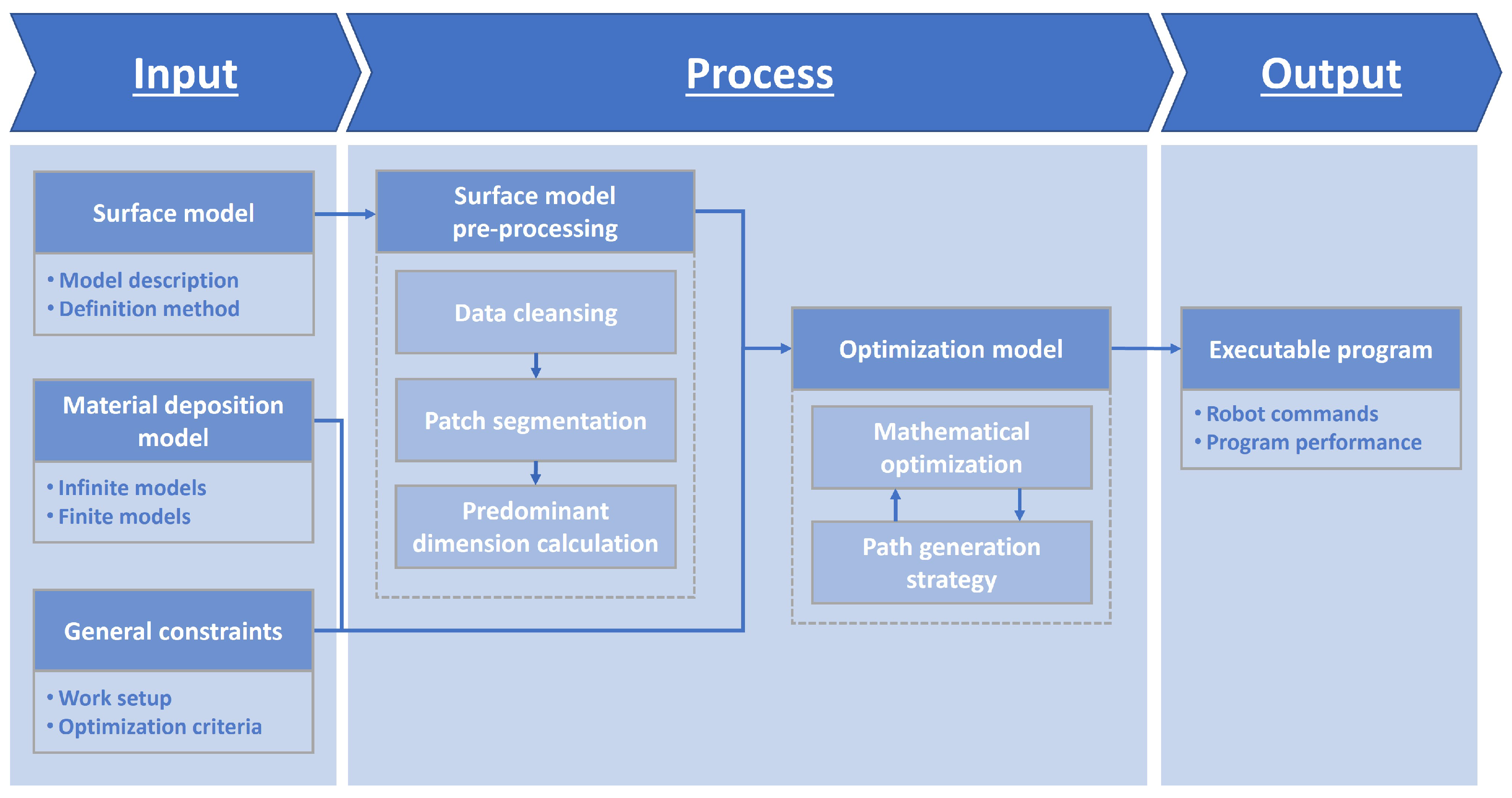
1.2. Overview

This paper provides a state-of the-art literature survey on the topic of robotic path generation for spraying applications. It aims to categorize the conceptual developments and provide a succinct summary of these frameworks that have emerged in this area of study. Four scholarly databases (Google Scholar, Scopus, IEEE Xplore, and ResearchGate) were used to download research papers that were published between 1982 and 2022. A reference repository has therefore been established, which includes 110 papers published in 68 scholarly journals and conference proceedings.

Most publications focus on specific subprocesses, and others include more integral concepts. But none fully solves the end-to-end path generation problem of complex surfaces [5]. However, at the core of most existing concepts lies a framework first presented by Heping Chen [9], which follows the basic input–process–output (IPO) model from software engineering. As this is the essence of most frameworks for path generation, this paper follows the same structure.

Figure 1 summarizes, in a flowchart, the building blocks of the framework and their interconnections, which are required to autonomously generate the spraying program. Each component will be explained in the following sections. In particular, Section 2 gives an overview of the required inputs and their alternative approaches to define them. In Section 3, the existing (sub-)algorithms are explained and their respective strategies are compared. The result of the calculation of the offline programming and simulation is further detailed in Section 4. Section 5 concludes the article.

2. Input Data

As illustrated in

Table 1. Required inputs for the path-generating algorithm.

Input	Category	Subcategory
Surface model	Model description	Parametric model
		Tessellated model
	Definition method	CAD-based
		Sensor-based
Material deposition model	Infinite models	Gaussian model
		Cauchy model
	Finite models	Trigonometric model
		Piecewise model
		Ellipse model
		Parabolic model
		Beta model
		Elliptical double beta model
General constraints	Work setup	Robot type
		Coating tool
		Workpiece properties
		Coating material
		Environmental conditions
	Optimization criteria	Operational requirements
		Coating quality
		Machine behavior

, there are multiple inputs that include the required information for the path-generating algorithm to propose a spraying program. These can be subdivided into the surface model, material deposition model, and general constraints. The first input includes the geometry and pose (i.e., position and orientation) of the workpiece and the data acquisition alternatives. The second input describes the shape of the spray cone and its projected material quantity at each position on the workpiece surface. In the third, other factors are listed that restrict the trajectory generation algorithm and its ability to be executed. In this section, all of the needed inputs, their alternative representation models, and the data acquisition options will be described.

2.1. Surface Model

The most basic criterion for determining the ideal trajectory of the spraying robot is the geometry of the workpiece’s surface. The reason for this is that only by knowing how the surface is defined is it possible to guarantee that the spraying tool covers its entirety with a uniform layer of coating material. Before being able to feed this information to any algorithm, two definitions need to be made: (1) in which format is the surface information represented and (2) how it is acquired. In Section 2.1.1, the former will be explained, while in Section 2.1.2 the latter will also be described.

2.1.1. Model Description

The model description of the surface focuses on how the data can be represented for further processing. This is important since it allows all of the different algorithms used by the path generating framework to correctly interpret what the workpiece looks like and ensure the accuracy of its trajectory calculations. There are two digital formats used for spraying applications: parametric models and tessellated models.

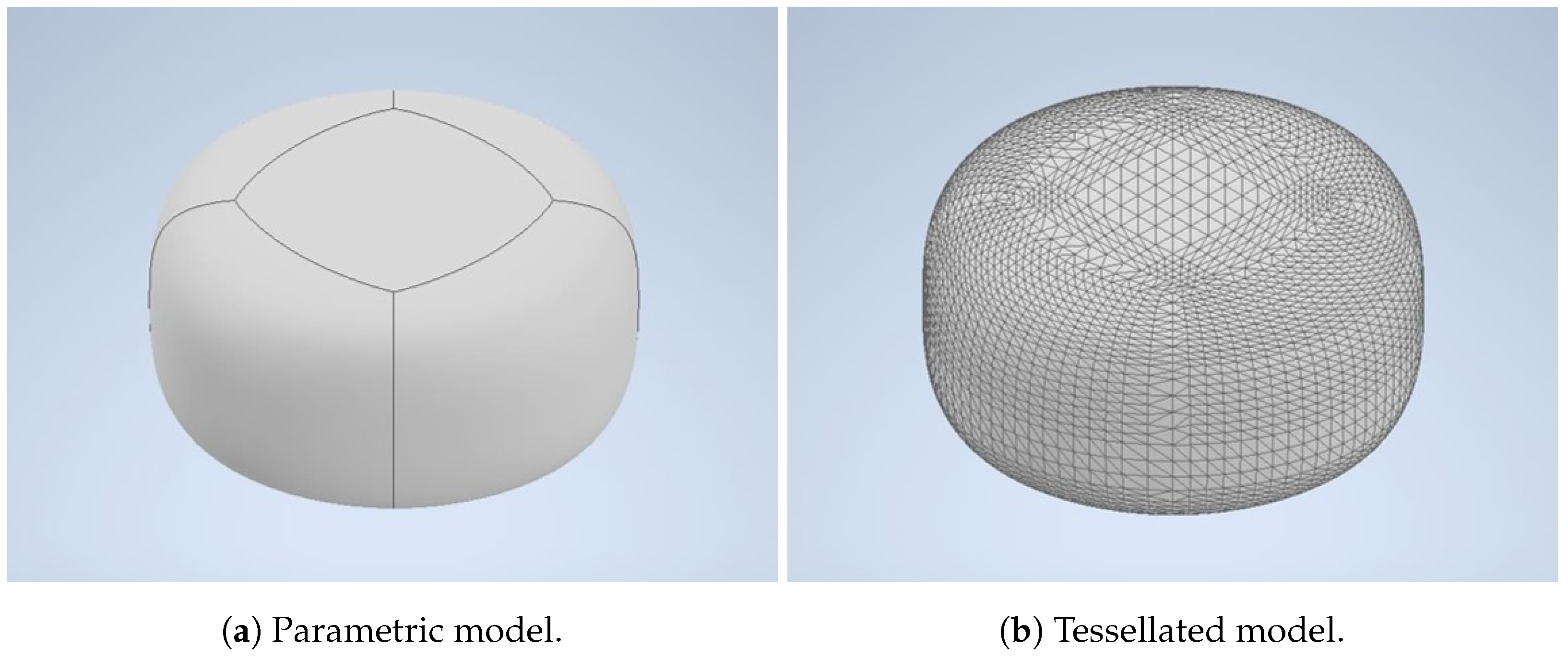
• Parametric models are a modeling paradigm based on parent–child interdependencies between features to generate a representation of the surface [10]. Parameters constitute the constraints that define the workpiece and can be dimensional, geometric, or algebraic. This modeling format constitutes the current industry standard for generating CAD-based parts and assemblies. With this format, it is possible to make a representative model while using supporting points, lines, arcs, splines, NURBS surfaces, and solid elements. This methodology guarantees a high level of accuracy in the representation of the design. However, there is much redundant information generated, a discretization step is required to calculate the spray coverage area, and each surface is interpreted independently, making an analysis of the entire surface more complex [11]. A typical example of the type of CAD file is STEP (the standard for the exchange of product model data), which is represented in Figure 2a.
• Tessellated models consist of generating a discrete surface representation with a 3D mesh of small elements (typically triangles or other polygons) [12]. This modeling method is the simpler alternative for analysis because the normal, location, and area of each element are directly known; the tessellated part can be considered as one piece; and it can achieve a good balance between representation accuracy and computation time. On the downside, there can be a lack of information on geometrical features such as edges, and the size of the data can become quite large, especially when high resolution is required (e.g., to represent large and/or complex parts) [11,12]. A typical CAD file format type is STL (standard tessellation language), as represented in Figure 2b.

2.1.2. Definition Method

An accurate depiction and model of the surface are essential for calculating the optimal path. Otherwise, the even coverage of the entire surface cannot be guaranteed, or in an extreme case, even a crash between tool and surface can occur. In this section, the digitazation procedures for measuring the surface shape of the workpiece are described, and their benefits and drawbacks are also listed. With this information, the data can be converted to one of the previously explained surface modeling formats. The two approaches taken in the literature to depict the surface of the workpiece are the CAD-based method and the sensor-based method.

• CAD-based method: In this approach, the blueprint of the workpiece, particularly the computer-aided design (CAD) file, is directly inserted into the trajectory calculation algorithm. This approach requires that the CAD-model is available, or else it needs to be created manually starting from the workpiece that needs to be sprayed [13]. This is the most common approach employed in publications to date for the following reasons [14]: (1) its simplicity in importing directly the model into the simulated environment and algorithm; (2) no measuring inaccuracies occur, as the workpiece trajectory is calculated directly out of the flawless CAD design; (3) the ease of the CAD-software converting automatically between the tessellated and parametric models as needed; and (4) it does not require the use of gauges and sensors to determine the surface geometry. The disadvantages of employing this method are (1) manufacturing inaccuracies can no longer be compensated for with path adaptations as the trajectory is generated for the “ideal” part; and (2) the pose (i.e., position and orientation) of the workpiece needs to be determined in the workcell before starting the spraying job, either by using a bracket to always hold the workpiece in the same pose, or by the use of gauges, to determine the exact placement [3].
• Sensor-based method: The alternative approach consists of measuring the real, to-be-coated workpiece, before initiating the computation of the spraying trajectory [13]. The advantages of this type of approach are [14]: (1) its flexibility, as no CAD data are required for the particular workpiece, and (2) that the actual workpiece surface measurements are introduced into the simulated environment and algorithm instead of those of a hypothetical model. On the other hand, (1) gauges are required to perform these measurements and (2) additional computational effort is needed to reverse engineer the surface [15].
  Different technologies can be used to make measurements in the sensor-based method:

  (a)

  Optical barriers: Gasparetto et al. [16] propose an image acquisition based on optical barriers to determine the geometry of the surface. This type of gauge consists of a light emitter and a receiver, which have a workpiece in between. The beam of light is interrupted by the workpiece, and therefore the position of the edges and the body can be determined. On the downside, this method only works for flat (2-dimensional) surfaces and by having the surface positioned at a known distance from the camera since the created shadow does not contain any depth information.

  (b)

  Depth camera: A different approach is presented by Tadic et al. [17], which includes the use of a depth camera. This type of camera generates a point cloud, which is an unorganized set of discrete points in a three-dimensional space. There are three types of depth camera technologies: stereo vision, structured light, and time-of-flight (ToF).

  Stereo vision systems use two separate cameras to capture an image from two positions. By knowing the distance between the cameras and comparing both signals that were recorded from different angles, it is possible to extract the depth information [18].

  Structured light systems, on the other hand, use light patterns that are emitted from a projector onto the workpiece’s surface. This pattern is distorted on the reflecting surface and then recognized by a sensing camera located in a different position. Following the same principle as stereo vision systems, triangulation enables the sensor to determine the 3-dimensional position of each point [18].

  Finally, ToF systems work based on an emitter that sends a pulsed signal directed toward the workpiece, and a receiver that measures the reflected light. By calculating the time difference between the emitted and received signal, it is possible to define the distance between the camera and the workpiece surface, thus gaining information on the third (depth) dimension [18].

  With the information from the point cloud gathered, it is now possible to digitally rebuild the measured surface. However, low-resolution depth cameras can lead to the misinterpretation of complex workpiece surfaces because only discrete points are recorded. At the same time, with high-resolution depth cameras, the computational effort increases drastically due to the large amount of data processing. Therefore, it is critical to find an adequate resolution for each application so that both factors (accuracy vs. computational effort) can be balanced out.

  (c)

  LiDAR: Light detection and ranging (LiDAR) is a type of sensor used for depth perception that works under the same principle as the ToF depth camera. Fundamentally, it measures the time interval between the emission and reception of a light pulse and then converts it into a distance. This system’s components include an emitter of laser pulses, a scanning system for redirecting the light onto the to-be-measured area, a detector for capturing the reflected light, and a processing unit to analyze the data. The sensor measures the scene by redirecting the laser beam across the measured area via the scanning mechanism, thereby identifying the surface coordinates and generating a point cloud [19].

  (d)

  Coordinate measuring machine: The third system-type that can be used for digitization of the workpiece is based on a coordinate measuring machine (CMM). In this case, a contact sensor (e.g., touch trigger probe) or non-contact sensor (e.g., laser) is attached to a robot, which moves the gauge in relation to the probe, thereby defining the point cloud coordinates [15]. Although a workpiece surface reconstruction can be created based on the information gained from a touch-trigger probe-based system, it is uncommon due to the data-acquisition time necessary for each coordinate and simultaneously the quantity of data-points required to recreate the surface with sufficient accuracy. Therefore, it is more common (and appropriate) to use non-contact sensors, as documented in the literature [13,20,21].

2.2. Material Deposition Model

The second main input according to Chen is the material deposition model [9]. Depending on the type of tool, its configurations, and its settings, the cone formed can have very different material deposition distributions in the sprayed area. Therefore, a mathematical model is required to accurately describe the shape of the spray cone and enable the calculation of the layer thickness at every position of the workpiece’s surface.

Chen proposes the framework shown in Figure 3a. The spraying material is emitted from the tool and generates a cone with a fan angle $\Phi$, which is projected onto the surface of the workpiece. At a predetermined tool standoff h, a spray pattern with radius R is generated.

Because the sprayed area can include non-flat sections, the spray cone from the tool model is then projected onto a free-form surface, as illustrated in Figure 3b. The calculation of the layer thickness at any point of the surface must therefore consider the distribution of the coating material in the cone, uneven surfaces, variations in the tool’s distance to the surface, and the angle towards the workpiece. Furthermore, the relative position of a specific surface point to the tool changes dynamically during the painting task as the tool moves to cover the entire surface. This means that each point will be covered with varying amounts of coating material at each instant while inside the spray-cone area and possibly even multiple times in the overlapping spraying areas. Therefore, it is also necessary to accumulate the amount of material deposited during the time each surface point has been sprayed to determine the final layer thickness of the coating. Chen proposes Equation (1) to calculate the material thickness on the surface $q_s$ [9]. This material thickness cannot be recognized on Figure 3a to simplify the sketch.

$$q_s=\left\{\begin{array}{cc}\overline{q}{\left(\frac{h}{l_i}\right)}^2\frac{cos{\gamma }_i}{co{s}^3{\theta }_i}& {\gamma }_i\le {90}^{\circ }\\ 0& {\gamma }_i>{90}^{\circ }\end{array}\right.$$

(1)

The variables to solve this equation are the material thickness on a plane $\overline{q}$, the distance $l_i$ of the tool to the measured point $s_i$, the deviation angle from the gun direction ${\gamma }_i$, and the deviation angle ${\theta }_i$ from O to $s_i$. The condition of having ${\gamma }_i$ below 90° guarantees that only material deposition with the spray tool directed toward the surface is taken into account. The variable $\overline{q}$ mathematically describes how the amount of coating material decreases within the sprayed area with the distance from the vertical projection point O. The two constant reference distances for each distribution model are the maximum at point O, and a hypothetical and non-existing material deposition (zero) when the distance is equal to the radius R.

There are multiple distribution models in the literature that describe the shape and size of the spray cone. This, for instance, quantifies how the amount of deposited material $\overline{q}$ decreases with increasing distance from point O and how the sprayed surface area expands when the spraying tool moves further away from the workpiece’s surface. Chen classifies these models as follows [22]:

• Infinite-range models: This type of model has non-zero values outside the range R. This means that the surface area outside the spray cone always has a very small amount of material deposited, which decreases further with the distance from point O. It includes, e.g., the Gaussian model and the Cauchy model.
• Finite-range models: Unlike the former, this type of model does not have material deposition outside the area delimited by the range R. It includes, e.g., the trigonometric model, the piecewise model, the ellipse model, the parabolic model, the beta model, and the elliptic double beta model.

The most commonly used models are from the finite-range model category, particularly the beta model and the elliptic double beta model. This is because both provide an adjustable and more accurate representation of the real spray cone when compared to most models [22]. In the following subsection, both will be further detailed.

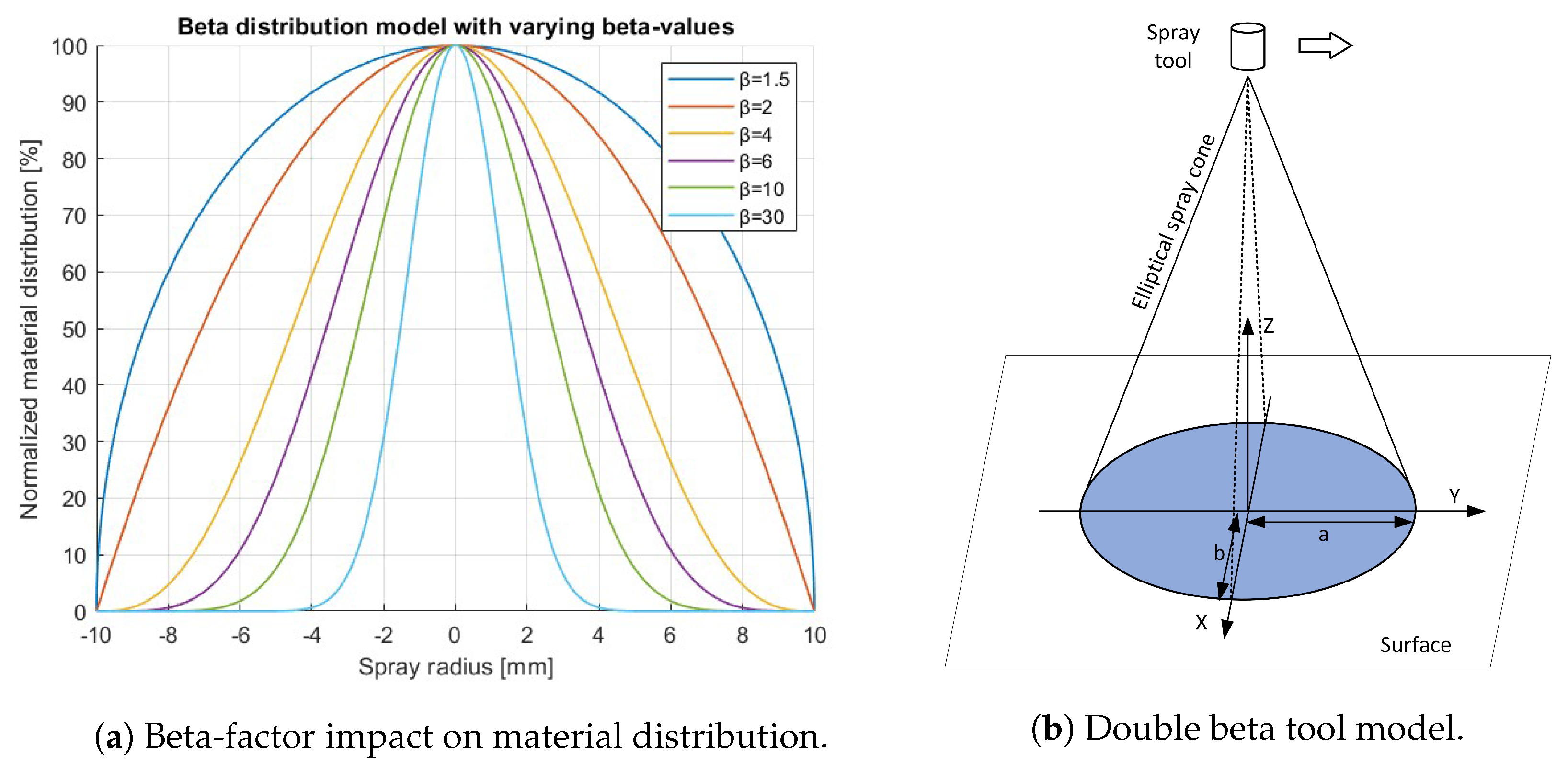
2.2.1. Beta Distribution Model

One of the most widely used material deposition models is the beta model [23]. The main factor leading to this is the model’s flexibility to adjust the shape of the spray cone. By changing the shaping parameter $\beta$, it is possible to fit the mathematical model to represent different spray cone shapes and therefore approximate the representation more accurately to the one generated in reality. Equation (2) describes the beta model.

$$\frac{\mathrm{d}\overline{q}\left(r\right)}{\mathrm{d}t}=\frac{\eta Q_0\beta }{\pi R^2}{\left(1-\frac{r^2}{R^2}\right)}^{\beta -1}$$

(2)

In this equation, the paint transfer efficiency is represented by $\eta$ and the spray gun paint flow rate is the variable $Q_0$. Figure 4a highlights the different shapes the spray cone can have depending on the shaping parameter $\beta$. Depending on the type of spray cone generated by the spraying system setup, the beta model can be adjusted to represent, e.g., an elliptical ($\beta =1.5$), parabolic ($\beta =2$), or Gaussian model ($\beta \ge 6$).

2.2.2. Elliptic Double Beta Distribution Model

This model is built on beta distribution model, but with the distinction that an elliptical area is generated on the hypothetic flat surface instead of a circular one; see Figure 4b. Equation (3) provides the definition by Zhou et al. to determine the material distribution for the elliptic double beta model [24].

$$\frac{\mathrm{d}\overline{q}(x,y)}{\mathrm{d}t}=d_{max}{\left(1-\frac{x^2}{a^2}\right)}^{{\beta }_1-1}{\left[1-\frac{y^2}{b^2\left(1-\frac{x^2}{a^2}\right)}\right]}^{{\beta }_2-1}$$

(3)

In this case, x and y represent the distances from point O in a Cartesian coordinate system, $d_{max}$ represents the maximum coating thickness, a and b represent the length of the long and short axis of the ellipse accordingly, and ${\beta }_1$ and ${\beta }_2$ are the shaping parameters for the ellipse on the long and short axis.

2.3. General Constraints

The third input category with the information required for the autonomous path generation of spraying tasks is general constraints, which includes the remaining restricting factors that affect the path generation. They depend on the work setup and on the optimization criteria chosen by the enduser [25]. These constraints remain unchanging for the coating jobs under stable processing conditions and are heuristically assumed to be constants in most of the algorithms developed.

2.3.1. Work Setup

The existing work setup is a constraining factor that must be considered when calculating a spray path. Although in theory it is possible to calculate all trajectories without this information, it is only possible to confirm that it can be run on the particular setup if all these constraints are considered. Take, for instance, the robot reachability—if a path goes outside the system’s reach, then the program cannot run for that particular setup. Therefore, this information is necessary to ensure compatibility with an existing configuration. Arikan and Balkan list the following setup criteria as factors affecting the spraying process [6]:

• Robot type: As was stated in the previous example, the robot or robots (when used in tandem as proposed in [14,26]) have an important impact on the compatibility of the generated path. Particularly the technical specifications of the robot, its configuration, its reach, and its kinematic behavior may require some program adaptations for the suggested path to be compatible with the existing setup. Although industrial robots are the most common type of system used for moving the spraying tool to cover the surface in an industrial setting, there are also alternative systems such as unmanned aerial vehicles (UAVs) for painting surfaces directly from the air [27,28].
• Coating tools: This input also restricts how the path needs to be calculated. The technical specifications of the coating tools, their type, their volumetric flow rate, and the tank pressure are examples of inputs that must be considered.
• Workpiece properties: Besides the surface model, there are also other properties related to the workpiece that limit the path compatibility. The surface roughness, the workpiece temperature, and its material are criteria that ultimately influence how well the sprayed coating material adheres to the workpiece surface.
• Coating material: With respect to the adherence of the coating material, not only the workpiece itself but also the coating material must be considered. The chemical composition, its physical state, its temperature, and its viscosity are examples of relevant factors.
• Environmental conditions: Finally, the workcell conditions, including the temperature, humidity, and atmospheric pressure, also condition the general coating process.

2.3.2. Optimization Criteria

The second type of constraint delimits the acceptable paths based on the optimization objectives. It not only restricts which paths can be used for a particular spraying task but also defines criteria to rank them against competing alternatives. An example would be a path that results in a uniform coating layer and has a minimal amount of coating material used; it should take preference over one with a less even distribution, and where more spraying material is wasted (e.g., by not being correctly aimed at the workpiece surface). These criteria must be predetermined and weighed against each other, limits must be established, and inputs must be included into the algorithm, so they can finally be added to the optimization model, described in Section 3.2. In the following, these preference criteria for the optimization model are listed:

• Operational requirements: This type of criterion focuses on improving the overall performance of the spraying process. The length of the trajectory and the cycle time needed to perform the job [9,29], and wasted materials [30] are key performance indicators (KPIs) evaluated in the literature to reach the (semi-)optimal trajectory.
• Coating quality: One of the main goals of fully automating spraying processes is to guarantee consistent and high-quality results for the sprayed workpiece. The quality of the coating depends on two measures: the coverage of the surface area and the uniformity of the coating thickness [9,31].
• Machine behavior: Finally, the parameters related to the machine behavior should also be considered to optimize the recommended path. Depending on the kinematic and dynamic behavior of the robot [32], and on the energy consumption of the system [33] a better path can be generated to spray a particular workpiece.

3. Processing Algorithm

After considering all the required input from the geometry of the workpiece, the material deposition model, and other constraints, it is now the task of the algorithm to convert all the acquired information into a program. This program includes all the information on the trajectory and orientation that the spraying tool needs to follow at any given point in time, as well as other relevant parameters to optimally spray the workpiece. Two processes need to be executed to generate the final trajectory for the spraying robot to follow, namely, surface model pre-processing and the optimization model.

Table 2. Algorithms needed for processing the input data into an executable spraying path.

Process	Category	Subcategory
Surface model pre-processing	Data cleansing	Outlier elimination
		Surface smoothing
		Data merging
		Data compression
		Format conversion
	Patch segmentation	Surface normal clustering
		Watershed segmentation
		Trapezoidal decomposition
		Boustrophedon decomposition
		Morse-based cellular decomposition
		Landmark-based topological coverage
		Minimal sum of altitudes (MSA) decomposition
	Predominant dimension calculation	Principal component analysis (PCA)
Optimization model	Mathematical optimization	Trajectory optimization
		Processing time optimization
		Coating quality optimization
		Kinematic and dynamic behavior optimization
	Path generating strategy	Slicing-based models
		Section-based models
		Differential geometry-based models

highlights these process steps and their respective algorithm categories and subcategories.

3.1. Surface Model Pre-Processing

Before the path generation algorithm can be executed, some data pre-processing steps need to be completed. The main goal behind this is to guarantee that the path-generating algorithm has accurate data with which subsequent processes can work and, at the same time, to avoid creating unpredictable behavior for the automated spraying process [15].

There are three steps that are executed to ensure the integrity of the data and bring it to an adequate format for further processing. First, the correctness of the data must be checked in a data cleansing step. Then, it is necessary to simplify complex surface information into elemental patches that can be processed by the path-generating algorithm. Finally, the predominant dimensions of each patch must be calculated to determine the best direction that the spraying strokes should take and thus minimize the number of turns required. All these steps will be further detailed in the following subsections.

3.1.1. Data Cleansing

When applying gauges to measure any type of physical attribute, there is always the possibility of measurement errors occurring. They can occur for a multitude of reasons (e.g., the technical limitations of the system itself or misuse by the operator), and they may skew the results from the algorithm, consequently impacting the spraying process itself and the coating quality. It is therefore important to validate the data and perform a data-cleansing step in sensor-based applications, particularly with point-cloud-based surface measurements. The following tasks must be performed to guarantee an accurate surface representation for all subsequent algorithms:

• Outlier elimination: Invalid data points and gross outliers must be identified and filtered out. A statistical filter can be used to remove unnecessary and noisy data, e.g., by computing the mean and standard deviation of the closest neighbors and pruning those values that lie outside a threshold criterion [17].
• Surface smoothing: A point cloud smoothing step is also recommended, so the surface representation becomes more uniform, resulting in straighter trajectories with simpler commands for the machines that execute the program [13]. Gaussian smoothing can be used for this purpose [34].
• Data merging: If multiple sensors are used, all datapoint information should be merged into one common coordinate system so that the workpiece can be analyzed as a whole [14].
• Data compression: A compression (or simplification) of the amount of data is required when the accuracy of the surface representation can be ensured [13]. This is an important step because depending on the resolution of the hardware used to generate the point cloud, large amounts of data-points can be defined, which will drastically increase the computational effort.
• Format conversion: And finally, a surface reconstruction should take place to bring the point cloud information to the right format for further processing by the following algorithms [14].

3.1.2. Patch Segmentation

The available algorithms for trajectory generation require a certain degree of simplicity to recognize how to proceed adequately on a particular surface and then create consistent and replicable results. Unfortunately, not all workpieces adhere to this and can only be described as complex surfaces. These types of surface need therefore to be broken down into simpler subsections, which then can be interpreted by the algorithm as a surface composed of elemental patches.

Figure 5a shows how the surface of an L-shaped workpiece could be subdivided into patches. There are two types of subdivision that can be recognized in the example.

The first is when two adjacent flat surfaces have a surface curvature exceeding a certain limit. For the part, this would be represented by the relation between patches D and E. The algorithms that assist in this segmentation are presented by Heping Chen [9], where the normal vectors of the neighboring surface are compared to each other, and if the value exceeds a certain threshold a new patch is generated. Nguyen and Lee present an end-to-end method for patch segmentation based on surface normal clustering [34]. Alternatively, the watershed segmentation algorithm can help restrict regions of high curvature and separate them, as suggested by Atkar et al. [30].

The second type is when the geometry and connectivity of the surface changes during the sweep. This can be exemplified in the relation between patches A and B, where the longer vertical section of the L is differentiated from the shorter horizontal part. Algorithms that help to calculate this type of segmentation are classical exact cellular decomposition methods (e.g., trapezoidal decomposition, boustrophedon decomposition) [30,35,36], Morse-based cellular decomposition [35], landmark-based topological coverage [35], or minimal sum of altitudes (MSA) decomposition [37]. These algorithms are not further elaborated to avoid overextending this section.

The importance of patch segmentation lies not only in pre-processing the surface data for the following algorithms but also in increasing the efficiency of the spaying program overall. Figure 5b highlights the impact of creating two patches from the same workpiece. The left picture shows a less efficient solution, where several turns are required to completely cover the surface of the workpiece. The image on the right shows how segmenting the surface creates longer paths with fewer turns, making this a less time-consuming and coating-material-saving approach.

3.1.3. Predominant Dimension Calculation

After generating patches from the workpiece surface, the predominant dimensions of these new elemental sections need to be determined. In this step, the longest surface dimensions of each patch must be identified in a newly set coordinate system so the straightest path can be selected as the direction of the spraying stroke. The principle component analysis (PCA) is the main approach used in the literature to determine the predominant dimensions of the patches [38]. It can help determine the dominant eigenvectors of the surface represented in the patch and thus make a recommendation for the longest straight path the spraying strokes could have.

This is a relevant step to support the following algorithms in identifying preferred paths more efficiently and to increase the speed of calculating a (semi-)optimal solution. Figure 6 illustrates to the left how an inefficient program can be generated if the predominant dimension is not selected. In the right case, the spraying direction of the sweeping algorithm is aligned with the longest dimension of the patch, thus reducing the number of required turns and increasing the process efficiency.

The orientation in which these (semi-)parallel spray painting strokes are performed affects not only the required processing time of the spraying; it also affects the amount of coating material used, due to the reduction material being pointed toward the outside of the surface area, and the surface quality of the workpiece due to the reduction in overlapping spraying strokes [39]. These are the main criteria that underline the importance of determining the longest straight pathways for the strokes in each individual patch.

3.2. Optimization Model

When using any particular path generation procedure, there are multiple settings and parameters that must be predefined for the algorithm to be executable. Defining the best (or even semi-optimal) configuration is a challenging task because these inputs are interrelated in complex manners and have varying impacts on the end result. Take, for instance, the tool standoff h, which, when increased, enlarges the sprayed area. This consecutively impacts the required distance between two adjacent paint strokes and can result in a new coating thickness variation over the workpiece’s surface.

Therefore, it is necessary to complement the path-generating algorithm with an overlying function that supports determining how inputs can be optimized with the aim of achieving the best possible result [5]. From a programming perspective, this could be considered a wrapper function that calls on any selected path-generating subroutine (i.e., the path generation strategy from Section 3.3) with a set of parameters and settings, so the result can then be compared with other configurations.

The primary approach described in the literature to solve this multiobjective optimization problem is mathematical optimization. This framework describes both the objective functions and the restrictions and finds the best solution while considering the general contraint inputs from Section 2.3. Different optimization models are proposed in the literature, and in the following section three of them will be explained: Section 3.2.1 Trajectory Optimization, Section 3.2.2 Processing Time and Surface Finish Optimization, and Section 3.2.3 Robotic Arm Kinematic and Dynamic Optimization.

3.2.1. Trajectory Optimization

One proposed method consists in optimizing the generated trajectory by reducing the number of required turns and consequently the processing time of the spraying job [37]. The core of this model lies in the use of the patches defined in the previous steps and the determination of the optimal starting and end points of the trajectory from potential candidates lying in the corners of the patch. Figure 7 illustrates how selecting different start- and end-points changes the spraying path. On the left figure, start-point (1) and end-point (4) were selected, resulting in three required strokes to cover the entire surface. Meanwhile, in the right figure, start-point (1) and end-point (3) are selected, which leads to two strokes to cover the surface. Under the assumption that equivalent coating layers are required, adaptations in tool speed and tool standoff h are needed when going from the left case to the right case, particularly due to the increase in spray width d (distance between adjacent strokes).

In Figure 8, the impact of setting the spraying direction is highlighted. Although in both cases the start- and end-points are (1) and (4), in the left case the direction was defined according to the predominant dimension and thus had the need for only three strokes, instead of 5 as in the right case. Taking the direction of the longest dimension of the patch is therefore the more efficient way to spray the surface, when the patch is being analyzed individually.

However, selecting the ideal points for each individual patch does not necessarily optimize the result for the entire spraying job. It is also critical to consider the connectivity between patches when calculating the best solution. Figure 9 exemplifies a scenario with the same patch as in Figure 8, where it is beneficial to have non-optimal trajectories inside some of the patches because then the travel distance between adjacent patches can be reduced. In this case, by using the non-optimal direction for patch B it is possible to reduce the number of required strokes from 11 (left) to 5 (right).

This optimization problem is a variation of the traveling salesman problem [29]. In Equation (4), the problem is described with the following variables: $v_i$ and $v_j$ represent two different vertices (i.e., potential start or end points), $g_k$ represents a group (i.e., patch), m is the number of vertices in group k, n represents the total number of vertices, $x_{ij}$ is a connection matrix containing Boolean values to represent the connectivity between the vertices i and j, $d_{ij}$ is the edge cost (i.e., distance) between vertices of different groups, and $t_{ij}$ is the edge cost between vertices of the same group k.

$$\begin{array}{cc}\hfill min& F=\left\{\sum \sum _{1\le i\ne j\le n,\forall v_i\in g_k,v_j\notin g_k}{d}_{ij}{x}_{ij},\sum \sum _{1\le i\ne j\le n,\forall v_i\in g_k,v_j\in g_k}{t}_{ij}{x}_{ij}\right\}\hfill \\ \hfill \mathrm{s}.\mathrm{t}.& \sum \sum _{i\ne j}{x}_{ij}=2,\forall v_i,v_j\in g_k,k=(1,...,m)\hfill \\ \hfill & \sum _{j,i\ne j}{x}_{ij}\%2=0,\forall i,(i=1,...,n)\hfill \\ \hfill & \sum \sum _{i\ne j}{x}_{ij}=2,\forall v_i\in g_k,v_j\notin g_k,k=(1,...,m)\hfill \\ \hfill & \sum _{v_i\in S}\sum _{v_j\notin S}{x}_{ij}\le 1,S\ne ⌀,Sisasubtour\hfill \end{array}$$

(4)

To summarize the model of Equation (4), the objective function gives us a multiobjective optimization problem, where the criteria that need to be minimized are (A) the trajectory distance when moving between patches and (B) the trajectory distance inside the same patch to cover its entire surface. Constraints 1 and 2 ensure that only two points are selected for each patch (starting- and end-point). The third constraint guarantees that each patch is only covered once by the resulting trajectory, thus avoiding spraying the same section multiple times. And the fourth is a subtour elimination constraint that ensures that all patches are covered on the same route.

3.2.2. Processing Time and Surface Finish Optimization

The second model suggested by Heping Chen focuses both on reducing the processing time and improving the quality of the surface finish [9]. In this framework, the processing time is minimized by optimizing the trajectory and speed of the spaying tool. At the same time, the quality of the sprayed surface is improved by guaranteeing the coverage and uniformity of the sprayed material over the entire surface of the workpiece.

Equation (5) describes the optimization problem as defined by Chen. In the model, the following variables are used (unexplained variables can be found in Equation (1)): $q_d$ is the material thickness; $q_d$ is the desired material thickness; $\Delta q_d$ is the allowable tolerance for the material thickness deviation; P represents a path segment; $M_k$ represents the path subsegments of P; $d_k$ and $v_k$ are the distance and speed of the spraying tool at the kth segment, respectively; and $q_{max}$ and $q_{min}$ are the maximal and minimal acceptable material thickness values, respectively.

$$\begin{array}{cc}\hfill min& J=F(J_1,J_2,J_3)\hfill \\ \hfill \mathrm{s}.\mathrm{t}.& \left|q_j-q_d\right|\le \Delta q_d\hfill \\ \hfill \mathrm{with}& q_j=\sum _{k=1}^P\frac{d_k}{M_k{v}_k}\sum _{i=1}^{M_k}f\left(htan{\theta }_i\right){\left(\frac{h}{l_i}\right)}^2\frac{cos{\gamma }_i}{co{s}^3{\theta }_i}\hfill \\ \hfill & J_1=\sum _{k=1}^P\frac{d_k}{v_k}\hfill \\ \hfill & J_2=\sum _{j=1}^N{\left(q_j-q_d\right)}^2\hfill \\ \hfill & J_3={\left(q_{max}-q_d\right)}^2+{\left(q_d-q_{min}\right)}^2\hfill \end{array}$$

(5)

In the model, the objective function establishes the three criteria that require optimization: $J_1$ represents the processing time of the spraying job, $J_2$ is the average deviation of the material thickness over the entire surface (i.e., mean squared error), and $J_3$ represents the range of material thickness. The sole constraint defined for this model ensures that the material thickness is within a predetermined tolerance for the entire surface.

All these criteria make up the multiobjective optimization problem that can be solved using the no preference articulation, the priori articulation of preference, the progressive articulation of preference, and the posteriori articulation of preference [40]. Chen et al. select the no-preference articulation method, which minimizes the distance from the candidate solution to the utopian solution without setting any optimization preferences [29]. Alternatively, Heping Chen also solves the multiobjective optimization problem by using the weighted sum method (a posteriori articulation of preference approach), where particular optimization criteria are given weighting factors and prioritized against each other [9].

3.2.3. Robotic Arm Kinematic and Dynamic Optimization

A third criterion that requires optimization is the kinematic and dynamic behavior of the robot. Its importance is highlighted in Figure 10 with a situation where in the transition from patch A to patch B a radical shift in the tool orientation is required. No smooth transition would be possible in the limited space depicted in the left picture, leading to high accelerations by the robot. Consequently, the turbulences created by the high acceleration could modify the spray cone’s shape, and mechanical restrictions of the robot could make the trajectory (i.e., sharp turn) technically impossible or inaccurate. Smooth trajectories, which are processed at quasi-constant speeds and with limited accelerations, improve the uniformity of the coating layer, reduce the cycle time of the spraying process, and lead to energy-savings due to the reduction in the required torque [38,41].

To achieve a more stable dynamic and kinematic behavior, Deng et al. propose the method depicted on the right picture, where the tool starts progressively reorienting itself before and after the angled section with the patch transition [42]. This small deviation from the tool orientation in relation to the surface normal can be tolerated because the quality of the deposited material remains unaffected as long as this small deviation angle remains within the predefined threshold [43].

In this context, Hegels et al. propose the mathematical model that focuses on optimizing the kinematics and dynamics of the robot in general and on reducing the coating error [32]. The multiobjective optimization problem is defined in Equation (6). The following variables are used in the model: $\alpha$, $\beta$, $\gamma$, and $\lambda$ are non-negative scalar weighting factors; m represents the number of vertices in the mesh; $\chi$ is the spray gun path; $z_i\left(\chi \right)$ represents the calculated distribution of vertex-bound coating thickness for a particular path; $Z_i$ is the desired coating thickness; n is the number of poses in the path; $x_j$ represents the position of the spray tool; $q_j$, $r_j$, and $s_j$ are the three normalized basis vectors of the frame; ${\rho }_j$ is the pose vector; and $t_j$ is the time the tool needs to move from poses ${\rho }_j$ to ${\rho }_{j+1}$.

$$\begin{array}{cc}\hfill min& E_g=E_l+\lambda E_m=E_l+\lambda (\alpha E_a+\beta E_{aa}+\gamma E_c)\hfill \\ \hfill \mathrm{with}& E_l\left(\chi \right)=\sum _{i=0}^m{(z_i\left(\chi \right)-Z_i)}^2\hfill \\ \hfill & E_a\left(\chi \right)=\sum _{j=1}^{n-1}{∥e_{a,j}\left(\chi \right)∥}^2=\sum _{j=1}^{n-1}{∥\frac{x_{j+1}-x_j}{t_j}-\frac{x_j-x_{j-1}}{t_{j-1}}∥}^2\hfill \\ \hfill & E_{aa}\left(\chi \right)=\sum _{j=1}^{n-1}\left({∥e_{aa,q,j}\left(\chi \right)∥}^2+{∥e_{aa,r,j}\left(\chi \right)∥}^2+{∥e_{aa,s,j}\left(\chi \right)∥}^2\right)\hfill \\ \hfill & E_c\left(\chi \right)=\sum _{j=1}^{n-1}{∥e_{c,j}\left(\chi \right)∥}^2=\sum _{j=1}^{n-1}{∥\frac{x_{j+1}-x_j}{∥x_{j+1}-x_j∥}-\frac{x_j-x_{j-1}}{∥x_j-x_{j-1}∥}∥}^2\hfill \\ \hfill & e_{aa,q,j}\left(\chi \right)=\frac{q_{j+1}-q_j}{t_j}-\frac{q_j-q_{j-1}}{t_{j-1}}\hfill \\ \hfill & e_{aa,r,j}\left(\chi \right)=\frac{r_{j+1}-r_j}{t_j}-\frac{r_j-r_{j-1}}{t_{j-1}}\hfill \\ \hfill & e_{aa,s,j}\left(\chi \right)=\frac{s_{j+1}-s_j}{t_j}-\frac{s_j-s_{j-1}}{t_{j-1}}\hfill \end{array}$$

(6)

The objective function of the problem uses the already mentioned weighted sum approach from Section 3.2.2 to scale the multiple objectives into one function using non-negative scalar weights. The user thereby has the ability to prioritize any particular objective according to his requirements. The optimization of error value $E_l$ focuses on reducing the coating thickness, while the acceleration factor $E_a$, angular acceleration factor $E_{aa}$, and path curvature factor $E_c$ attempt to smooth the trajectory so that the kinematic and dynamic behavior of the robot is improved. The author does not include constraints in his mathematical formulation, although the reachability of the robot and the tool should be considered if optimizing the dynamic and kinematic behavior of the system.

3.3. Path Generation Strategy

At the center of the entire framework stands the algorithm to effectively determine the optimal path of the spraying tool. In the relevant literature, multiple strategies have been proposed to generate this program, starting from the required inputs, listed in Section 2, and they were finally turned into an executable program. These strategies provide an approach to guarantee that the entire workpiece surface is covered by the spraying material and infer the required path from this calculation. Three path-generating strategies will be presented in this section: Section 3.3.1, Section 3.3.2 and Section 3.3.3.

3.3.1. Slicing-Based Models

The main concept behind slicing-based models lies in having surface patches sliced by parallel-cutting planes to create supporting path sections or supporting points that will then, once joined, constitute the final path [44]. The distance between neighboring cutting planes is constant in most models, although it can be varied depending on the employed methodology. The supporting path segments or points are then determined by the intersection of the workpiece surface and the cutting plane. The resulting paths or points are then offset by the tool standoff h and afterwards interconnected in a meander-shaped order (i.e., with alternating direction between neighboring strokes) so that the final path can cover the entire patch in one go. This approach ensures that the distance between adjacent strokes remains uniform. Figure 11 illustrates the process, starting from the definition of equidistant section planes (i.e., $d_1$, $d_2$, and $d_3$ are constant) to the generation of the projected path and finally that of the tool path.

The bounding box method proposed by Sheng et al. was the first model to adopt the approach of this category [44]. It is named this way due to the cuboidal bounding box used to delimit the entire patch that is analyzed; see Figure 12. Three orthonormal vectors of the cuboid are determined and named the FRONT, RIGHT, and TOP directions. The FRONT direction of the bounding box corresponds to the opposite direction of the area-weighted average surface normal of the patch, and the RIGHT direction corresponds to the longest dimension direction of the patch [46]. Both vectors with the shortest lengths (FRONT and TOP) of the bounding box generate cutting planes that are offset by a distance of $d=\frac{2w}{d}$ throughout the RIGHT vector direction (i.e., the longest dimension of the patch) for the entire bounding box. Subsequently, the intersection path of the cutting planes and the surface is determined and all paths are connected to create a continuous path. Finally, the tool standoff h is added to calculate the tool path from the illustrated projected path.

Chen proposed a further development of the method to improve the strategy for dealing with irregularly shaped patches and named it the improved bounding box method [9]. The approach is illustrated in Figure 13. This method also uses the bounding box and cutting planes that are offset in the RIGHT direction. But unlike the original method, the entire intersection path of the surface and cutting-planes is not used as a path section. In this case, additional TOP cutting planes are offset by the spray width distance d from each other. The distance between the RIGHT planes, on the other hand, is adapted depending on the accuracy needs by the user, i.e., the smaller the distance between the RIGHT planes, the better the spraying coverage accuracy becomes.

The number of intersection points between the workpiece surface and the TOP and RIGHT planes is counted (in the figure, this is highlighted by the black points). Each RIGHT plane has a p value, which represents the number of strokes that must pass through that surface section. Subsequently, the intersection line between the RIGHT plane and workpiece surface is subdivided into equidistant segments with the same number of waypoints p, as highlighted by the blue rings in the sketch. This can lead to a shift in position from the planes’ intersection to the real waypoint, which is illustrated on planes $p_j$ and $p_{j+3}$. Finally, the points are interconnected following the RIGHT direction in a meander-shaped order, generating the projected path [46].

More recently, a method called the mesh-following technique was proposed by Mineo et al., which is a simplification of the improved bounding box method [47], with the difference being that no equidistant segments are required from the supporting curve generated by the RIGHT planes, thereby eliminating the need for the blue rings in the sketch. Alternatively, the black points are taken directly as waypoints to calculate the projected path the tool needs to follow.

The oriented bounding box method is another improvement to the original bounding box method, where with principal component analysis (PCA) the three predominant eigenvectors (i.e., dimensions of largest variation) are determined [38]. This approach proposed by Wang et al. ensures that the slicing plane is perpendicular to the direction of the longest axis. The authors also propose employing iterative adaptations to the distance between slices to allow for compensation in the curvature of the surface, thus ensuring coating thickness uniformity.

3.3.2. Section-Based Models

This type of model makes use of supporting poses (i.e., position and orientation) that the tool must pass to cover the entire surface of the workpiece. This concept first proposed by Bi and Lang requires a tessellated model description and involves two main tasks: first, determining a set of required poses (which are also named control-/way-/ or tag-/points) that ensure that the entire surface can be covered, and second, defining the optimal sequence for which these points are passed by the tool [14].

In this method, the mesh triangles that represent the workpiece surface are grouped according to the shape and size of the coating cone. The starting point is an extreme corner of the surface patch, and the neighboring triangles are added incrementally. Mesh triangles are included until an area equivalent to the coating area (represented by the blue circles) has been reached. With this selected area, a tool pose is then determined by calculating the center of this area and adding the predetermined tool standoff h in the direction of the weighted surface normal.

Afterwards, the same process is restarted for mesh triangles outside the previous areas until no more are left, and the surface is completely covered. Figure 14 illustrates how the tag points are determined in the surface mesh. The path must then be generated by defining the optimal sequence of the control points while ensuring that no collisions between tool, robot, and workpiece occur. Bi and Lang propose to formulate this task as a traveling salesman problem (TSP) to ensure that all points are covered while minimizing cost (in this case, the distance traveled).

An extension of this model is proposed by Andulkar and Chiddarwar [4]. In the new method, the mesh triangles are also filtered, starting with the distance from an initial corner. Neighboring mesh triangles within a predefined range are selected until the area reaches the size of the area covered by the spray cone. With this selected area, the center and surface normal are calculated and the tool standoff h is added to define the waypoint for the coating tool. However, unlike the previous model, now the filtered area is increased by an increment in the x-direction (assuming this is the longer dimension) to define the next pose. This pose definition step is then repeated until the border of the surface is reached.

At that point, the filtered area increases in the y-direction. Movement in the y-direction can be performed while spraying the workpiece (continuous raster pattern) or outside the surface area (discontinuous raster pattern), thus overpassing the surface area to some extent. Of these two alternatives, the latter is recommended by the authors because it ensures a more uniform layer thickness with minimal variation. This process is then repeated until all the mesh triangles on the surface have been covered and a final meander-shaped path has been generated. The benefit of the approach by Andulkar and Chiddarwar when comparing it to the one presented by Bi and Lang is that the first requires a tag-point-sequencing step to solve the TSP, while in the second, the sequence of poses is directly defined during the incremental expansion of the filtered surface area.

3.3.3. Differential Geometry Based Models

This third category of path generation methodologies uses differential geometry to generate the desired spraying path. The offset curve planner approach, as named by Atkar et al., is included in this category and uses geodesics (the shortest path between two points on a three-dimensional surface) to define the ”straightest“ path across the surface. The reason behind prioritizing a geodesic curve over others is its positive impact on the evenness of the paint deposition and the time it takes to complete the painting process [39].

There are two main steps in this method: first, determine the optimal starting curve (also called the seed curve), and second, generate the next strokes by offsetting them along the entire surface of the workpiece. The authors propose the application of the Gauss–Bonnet theorem to select the starting curve that minimizes the geodesic curvature of subsequent strokes and arrive at the conclusion that the best starting curve would be the Gaussian curvature divider. This curve should preferably be a geodesic, although it is not compulsory. The following offset curves are then determined by calculating the orthogonal geodesic to the starting curve and creating the new stroke at a uniform geodesic distance, which guarantees that the strokes are equidistant at all points, as depicted in Figure 15.

After all of the curves have been determined, they are then connected in a meander-shaped order, as was described for Slicing-Based Models in Section 3.3.1. The result of this procedure is the projected path on the workpiece surface, which then has to be offset by the tool standoff h to define the final tool path.

4. Computation Output

The output of the computation described in the earlier sections should be the best possible executable program for the robot to follow and process the particular spraying task. When analyzing the results of the algorithm, there are two components of the output that need to be considered: first, the information gained from the calculation must be translated into specific robot commands, so that the machine knows how to process the recommended path; second, an evaluation of the performance of the program should be made in a virtual environment to ensure that the results are in line with the expectations of the end user. Both these components are highlighted in

Table 3. Results of the algorithm for spray path generation.

Output	Category	Subcategory
Executable program	Robot commands	Waypoints coordinates
		Waypoint speed
		Waypoint acceleration
		Spraying tool angle
		Angular speed
		Tool status
	Program performance	Processing time
		Coating uniformity
		Coating coverage
		Spraying material wastage

and will be further described in this section.

4.1. Robot Commands

After the trajectory recommendation is calculated by the previous algorithms, it is time to transfer the data to the (real or simulated) robot for its subsequent execution. However, the format of the path information coming from the algorithm does not always correspond to that which is understood for the successive processing steps, leading to the difficulties in correctly compiling the robot program. For instance, if a path section is a curved line (e.g., a geodesic) described by its mathematical function, then subsequent programs would not necessarily know how to process this information. In this case, a discretization step is required to translate the information into supporting waypoints in the robot coordinate system [38]. An accurate replica of the algorithm’s recommended path should result from this discretization once all the waypoints are interconnected and passed in the predetermined sequence. For generating the robot-specific commands, additional inputs are necessary, which are listed below:

• Waypoint coordinates: These are specific positions through which the spraying tool must pass to properly coat the workpiece [48]. It is the first component of the pose and must include the Cartesian coordinates, which unambiguously define how the workpiece, robot, and tool are placed in relation to each other.
• Waypoint speed: The speed is also an important component of the calculation because it affects the amount of coating material deposited at each point of the workpiece surface. Although most models assume a constant speed for the entire path, in the case of varying speeds, it is necessary for the machine commands to include the particular speed-value for each waypoint [13].
• Waypoint acceleration: Analogously to the waypoint speed, the acceleration is also required to ensure the uniform deposition of the coating material on the surface [39]. This information will support minimizing sudden changes in the deposition rate and ensure the good adherence of the coating material to the workpiece surface.
• Spraying tool angle: The orientation of the spraying tool is the second component of the pose and complements the waypoint coordinate information. Only by defining how the tool is oriented with respect to the workpiece is it possible to guarantee that the coating material is correctly aimed at the surface, thus adhering to the surface efficiently and minimizing material waste [49].
• Angular speed: The angular speed with which the spraying tool changes its orientation should also be defined as an input. With limitations to this parameter, gradual angle changes can be implemented, which results in the better kinematic behavior of the robot and leads to a more uniform layer of the coating material [42].
• Tool status: The tool status defines in every waypoint if the spraying tool is active (meaning emitting spraying material) or disabled (the opposite). This information is used to reduce material waste, which is generated when the spraying tool is active while being aimed away from the workpiece surface (e.g., when moving to the first waypoint or changing the stroke direction) [13].

A post-processor must then take all this information and translate it into robot-specific commands in its native programming language [50]. With this input, it is finally possible for the robot driver to calculate via inverse kinematics, which angles and speeds the machine joints should activate at any given time, so the tool positioning recommendation can be followed as determined by the path-generating algorithm [51]. Different offline programming (OLP) solutions, CAM programs, or software libraries are used for this purpose in the relevant literature, with the most common examples for spraying applications being RobotStudio^™ [21,42,48,52,53,54,55], ROS/ROS2 [17] and RoboDK [13]. The different OLP tools are not further discussed to limit the size of this section. A comparative analysis between ROS and RoboDK (both being systems that are robot-agnostic, unlike RobotStudio^™) was published by Garbev and Atanassov [56].

4.2. Program Performance

The other output of the algorithm that comes jointly with the commands should be the associated assessment of the recommendation’s performance [14]. It is important that the operator has visibility of the end-result early on, to review it and to validate compliance with its own expectations. Some program performance criteria that constitute the KPI for the generated path and which were listed in Section 2.3.2 are processing time, coating uniformity, coating coverage, and spraying material wastage. This program validation ensures that the executable program is within the range of the expected process demands and quality requirements of the workpiece before carrying out the commands on the robot.

Simulation is a helpful tool for this analysis because it can help assess these criteria in a virtual environment and without the need for an expensive experimental validation [57]. The OLP tools and CAM software enable the end-user to first visualize the algorithm’s recommendation in a virtual environment that includes the robot with its tool and the workpiece. RobotStudio^™ and RoboDK, mentioned earlier, have these capabilities when importing workpiece data originating from a CAD-based input and running the program in a simulation. The conclusions that can be taken out of this process are not only that the recommended path is adequate but that it also helps the operator in identifying errors that can still be corrected with little effort, e.g., that the tool can reach all of the path’s points or foresee potential crashes [48].

The simulation is also used to predict the distribution of the coated material on the surface of the workpiece. For each mesh element, the associated layer thickness can be highlighted by color-coding its values in the visualization, as suggested in the literature [4,13,23]. Thus, the expert can instantly identify areas of the surface that were not adequately covered with the spraying tool or if the layer thickness distribution becomes uneven in certain segments, when using the recommended path. With this information, the expert is supported in the analysis whether or not the result is within the preset tolerances and meets expectations, while simultaneously being integrated into the decision-making process (i.e., human-in-the-loop).

5. Conclusions

Research led by industry and academia continues to investigate robotic-assisted spraying processes with the goal of one day making them fully autonomous, while being robust, reliable, and economical. Such an ideal solution would benefit not only large industry sectors (e.g., automotive and aeronautics) but also small and medium-sized businesses, which find it more difficult to afford high-end spraying work cells and professionals with the required engineering expertise. Although there are many parties interested in the technological progress of this field, to this day there is no commercially available end-to-end solution that automatically generates the spraying trajectory on complex 3D surfaces. Potential reasons for this are that the process stability for these highly complex spraying tasks cannot be guaranteed, the high level of customization in each machine setup, and difficulties in integrating all the needed components (i.e., hardware and software).

In this paper, a summary of recent research and literature is presented. The framework components have been classified according to the IPO model that Heping Chen follows, so each part can be mapped where it stands in terms of the complete solution and to compare alternative methodologies [58]. The inputs required for the path-generating algorithm are (1.1) the surface model representation of the workpiece, (1.2) a description of the material deposition model, and (1.3) a list of general constrains settings and parameters. This information is fed into the processing algorithm, where a (2.1) pre-processor cleans the data, segments them into simple patches, and calculates the predominant dimensions of each patch; (2.2) a mathematical optimization step is executed to determine the best-performing settings for the paths; and (2.3) trajectories are calculated following different strategies for path generation. The algorithm output is then presented as an executable program with (3.1) machine commands for the end-user to verify in a simulated environment based on the (3.2) program performance criteria.

Future work should first focus on building a holistic solution that includes all the required components analyzed in this paper. As there is still no such solution available, the focus should lie in creating such a package based on a system agnostic (i.e., one that is available for different types and brands of robots) and an open-source platform (e.g., ROS/ROS2), so the entry barriers are lowered and more parties can benefit from the technology. The path generation framework should also be coupled with the part recognition framework already mentioned in the literature, which suggests an expansion based on the workpiece being recognized and compared with existing workpiece-specific programs stored in a database [53,59].

Furthermore, concepts based on machine learning (ML) should also be studied to establish how they could be integrated into the framework. Posada et al. propose five different conceptual approaches that were not implemented and that have the potential to further improve the efficiency of the solution [5]. Helou et al. present an ML concept based on deep learning that infers robot commands from an ink map with a specific texture, although it is developed only for a 2D surface [33]. Finally, another option is the use of robot reinforcement learning as a policy-finding methodology, which could also be applied to spraying applications [50,51]. It is paramount to continue research in this field so that autonomous robot-assisted spraying applications become a reality, leading to the democratization of this indispensable manufacturing process.

References

- Quintino, L. Overview of coating technologies. In Surface Modification by Solid State Processing; Elsevier: Amsterdam, The Netherlands, 2014; Chapter 1; pp. 1–24. [Google Scholar] [CrossRef]
- Fauchais, P.L.; Heberlein, J.V.; Boulos, M.I. Thermal Spray Fundamentals; Springer: Boston, MA, USA, 2014. [Google Scholar] [CrossRef]
- Lin, W.; Anwar, A.; Li, Z.; Tong, M.; Qiu, J.; Gao, H. Recognition and Pose Estimation of Auto Parts for an Autonomous Spray Painting Robot. IEEE Trans. Ind. Inform. 2019, 15, 1709–1719. [Google Scholar] [CrossRef]
- Andulkar, M.V.; Chiddarwar, S.S. Incremental approach for trajectory generation of spray painting robot. Ind. Robot. 2015, 42, 228–241. [Google Scholar] [CrossRef]
- Posada, J.R.; Meissner, A.; Hentz, G.; D’Agostino, N. Machine learning approaches for offline-programming optimization in robotic painting. In Proceedings of the 52nd International Symposium on Robotics, ISR 2020, Munich, Germany, 17–18 June 2020; pp. 280–286. [Google Scholar]
- Sahir Arikan, M.A.; Balkan, T. Process modeling, simulation, and paint thickness measurement for robotic spray painting. J. Robot. Syst. 2000, 17, 479–494. [Google Scholar] [CrossRef]
- Conner, D.C.; Greenfield, A.; Atkar, P.N.; Rizzi, A.A.; Choset, H. Paint deposition modeling for trajectory planning on automotive surfaces. IEEE Trans. Autom. Sci. Eng. 2005, 2, 381–391. [Google Scholar] [CrossRef]
- Chen, H.; Thomas, F.; Xiongzi, L. Automated industrial robot path planning for spray painting a process: A review. In Proceedings of the 4th IEEE Conference on Automation Science and Engineering, CASE 2008, Mexico City, Mexico, 20–24 August 2008; pp. 522–527. [Google Scholar] [CrossRef]
- Chen, H. A General Framework for Automated Cad-Guided Optimal Tool Planning in Surface Manufacturing. Ph.D. Thesis, Michigan State University, East Lansing, MI, USA, 2003. [Google Scholar]
- Camba, J.D.; Contero, M.; Company, P. Parametric CAD modeling: An analysis of strategies for design reusability. CAD Comput. Aided Des. 2016, 74, 18–31. [Google Scholar] [CrossRef]
- Chen, H.; Fuhlbrigge, T.; Li, X. A review of CAD-based robot path planning for spray painting. Ind. Robot. 2009, 36, 45–50. [Google Scholar] [CrossRef]
- Guo, J.; Ding, F.; Jia, X.; Yan, D.M. Automatic and high-quality surface mesh generation for CAD models. CAD Comput. Aided Des. 2019, 109, 49–59. [Google Scholar] [CrossRef]
- Yu, X.; Cheng, Z.; Zhang, Y.; Ou, L. point cloud modeling and slicing algorithm for trajectory planning of spray painting robot. Robotica 2021, 39, 2246–2267. [Google Scholar] [CrossRef]
- Bi, Z.M.; Lang, S.Y. A framework for CAD and scanner-based robotic coating automation. IEEE Trans. Ind. Inform. 2007, 3, 84–91. [Google Scholar] [CrossRef]
- Mian, S.H.; Al-Ahmari, A. Comparative analysis of different digitization systems and selection of best alternative. J. Intell. Manuf. 2019, 30, 2039–2067. [Google Scholar] [CrossRef]
- Gasparetto, A.; Vidoni, R.; Pillan, D.; Saccavini, E. Optimal path planning for spray painting robots. In Proceedings of the ASME, Calgary, AB, Canada, 27 September–1 October 2010. [Google Scholar]
- Tadic, V.; Odry, A.; Burkus, E.; Kecskes, I.; Kiraly, Z.; Klincsik, M.; Sari, Z.; Vizvari, Z.; Toth, A.; Odry, P. Painting path planning for a painting robot with a realsense depth sensor. Appl. Sci. 2021, 11, 1467. [Google Scholar] [CrossRef]
- Zanuttigh, P.; Marin, G.; Dal Mutto, C.; Dominio, F.; Minto, L.; Cortelazzo, G.M. Time-of-Flight and Structured Light Depth Cameras; Springer: Cham, Switzerland, 2016; p. 355. [Google Scholar] [CrossRef]
- Raj, T.; Hashim, F.H.; Huddin, A.B.; Ibrahim, M.F.; Hussain, A. A Survey on LiDAR Scanning Mechanisms. Electronics 2020, 9, 741. [Google Scholar] [CrossRef]
- Candel, A.; Gadow, R. Trajectory generation and coupled numerical simulation for thermal spraying applications on complex geometries. J. Therm. Spray Technol. 2009, 18, 981–987. [Google Scholar] [CrossRef]
- Vincze, M.; Pichler, A.; Biegelbauer, G.; Hausler, K.; Andersen, H.; Madsen, O.; Kristiansen, M. Automatic robotic spray painting of low volume high variant parts. Int. Symp. Robot. 2002, 7, 11. [Google Scholar]
- Chen, Y.; Chen, W.; Li, B.; Zhang, G.; Zhang, W. Paint thickness simulation for painting robot trajectory planning: A review. Ind. Robot. 2017, 44, 629–638. [Google Scholar] [CrossRef]
- Andulkar, M.V.; Chiddarwar, S.S.; Marathe, A.S. Novel integrated offline trajectory generation approach for robot assisted spray painting operation. J. Manuf. Syst. 2015, 37, 201–216. [Google Scholar] [CrossRef]
- Zhou, B.; Fang, F.; Shao, Z.; Meng, Z.; Dai, X. Fast and templatable path planning of spray painting robots for regular surfaces. Chin. Control. Conf. 2015, 9, 5925–5930. [Google Scholar] [CrossRef]
- Chen, H.; Xi, N.; Sheng, W.; Chen, Y. General framework of optimal tool trajectory planning for free-form surfaces in surface manufacturing. J. Manuf. Sci. Eng. 2005, 127, 49–59. [Google Scholar] [CrossRef]
- Zbiss, K.; Kacem, A.; Santillo, M.; Mohammadi, A. Automatic Collision-Free Trajectory Generation for Collaborative Robotic Car-Painting. IEEE Access 2022, 10, 9950–9959. [Google Scholar] [CrossRef]
- Vempati, A.S.; Kamel, M.; Stilinovic, N.; Zhang, Q.; Reusser, D.; Sa, I.; Nieto, J.; Siegwart, R.; Beardsley, P. PaintCopter: An Autonomous UAV for Spray Painting on Three-Dimensional Surfaces. IEEE Robot. Autom. Lett. 2018, 3, 2862–2869. [Google Scholar] [CrossRef]
- Vazquez-Carmona, E.V.; Vasquez-Gomez, J.I.; Herrera-Lozada, J.C.; Antonio-Cruz, M. Coverage path planning for spraying drones. Comput. Ind. Eng. 2022, 168, 108125. [Google Scholar] [CrossRef]
- Chen, H.; Xi, N.; Sheng, W.; Dahl, J.; Li, Z. Optimal tool trajectory integration in surface manufacturing. IFAC Proc. Vol. 2005, 16, 211–216. [Google Scholar] [CrossRef]
- Atkar, P.N.; Conner, D.C.; Greenfield, A.; Choset, H.; Rizzi, A.A. Hierarchical segmentation of piecewise pseudoextruded surfaces for uniform coverage. IEEE Trans. Autom. Sci. Eng. 2009, 6, 107–120. [Google Scholar] [CrossRef]
- Chen, W.; Liu, J.; Tang, Y.; Huan, J.; Liu, H. Trajectory Optimization of Spray Painting Robot for Complex Curved Surface Based on Exponential Mean Bézier Method. Math. Probl. Eng. 2017, 2017, 4259869. [Google Scholar] [CrossRef]
- Hegels, D.; Wiederkehr, T.; Muller, H. Simulation based iterative post-optimization of paths of robot guided thermal spraying. Robot. Comput. Integr. Manuf. 2015, 35, 1–15. [Google Scholar] [CrossRef]
- Helou, M.E.; Mandt, S.; Krause, A.; Beardsley, P. Mobile robotic painting of texture. IEEE Int. Conf. Robot. Autom. 2019, 5, 640–647. [Google Scholar] [CrossRef]
- Nguyen, H.H.; Kim, J.; Lee, Y.; Ahmed, N.; Lee, S. Accurate and fast extraction of planar surface patches from 3D point cloud. In Proceedings of the 7th International Conference on Ubiquitous Information Management and Communication, ICUIMC 2013, Bali, Indonesia, 8–10 January 2013. [Google Scholar] [CrossRef]
- Galceran, E.; Carreras, M. A survey on coverage path planning for robotics. Robot. Auton. Syst. 2013, 61, 1258–1276. [Google Scholar] [CrossRef]
- Choset, H.; Pignon, P. Coverage Path Planning: The Boustrophedon Cellular Decomposition. Field Serv. Robot. 1998, 1, 203–209. [Google Scholar] [CrossRef]
- Huang, W.H. Optimal line-sweep-based decompositions for coverage algorithms. IEEE Int. Conf. Robot. Autom. 2001, 1, 27–32. [Google Scholar] [CrossRef]
- Wang, G.; Cheng, J.; Li, R.; Chen, K. A new point cloud slicing based path planning algorithm for robotic spray painting. In Proceedings of the 2015 IEEE International Conference on Robotics and Biomimetics (ROBIO), Zhuhai, China, 2 December 2015; pp. 1717–1722. [Google Scholar] [CrossRef]
- Atkar, P.N.; Greenfield, A.; Conner, D.C.; Choset, H.; Rizzi, A.A. Uniform Coverage of Automotive Surface Patches. Int. J. Robot. Res. 2005, 24, 883–898. [Google Scholar] [CrossRef]
- Andersson, J. A Survey of Multiobjective Optimization in Engineering Design; Technical Report January 2000; Department of Mechanical Engineering, Linktjping University: Linktjping, Sweden, 2000. [Google Scholar]
- Trigatti, G.; Boscariol, P.; Scalera, L.; Pillan, D.; Gasparetto, A. A new path-constrained trajectory planning strategy for spray painting robots. Int. J. Adv. Manuf. Technol. 2018, 98, 2287–2296. [Google Scholar] [CrossRef]
- Deng, S.H.; Cai, Z.H.; Fang, D.D.; Liao, H.L.; Montavon, G. Application of robot offline programming in thermal spraying. Surf. Coatings Technol. 2012, 206, 3875–3882. [Google Scholar] [CrossRef]
- Moe, S.; Gravdahl, J.T.; Pettersen, K.Y. Set-Based Control for Autonomous Spray Painting. IEEE Trans. Autom. Sci. Eng. 2018, 15, 1785–1796. [Google Scholar] [CrossRef]
- Sheng, W.; Xi, N.; Song, M.; Chen, Y.; MacNeille, P. Automated CAD-guided robot path planning for spray painting of compound surfaces. IEEE Int. Conf. Intell. Robot. Syst. 2000, 3, 1918–1923. [Google Scholar] [CrossRef]
- Atkar, P.; Choset, H.; Rizzi, A. Towards optimal coverage of 2-dimensional surfaces embedded in R3: Choice of start curve. In Proceedings of the 2003 IEEE/RSJ International Conference on Intelligent Robots and Systems (IROS 2003) (Cat. No.03CH37453), Las Vegas, NV, USA, 27–28 October 2003; pp. 3581–3587. [Google Scholar] [CrossRef]
- Chen, H.; Xi, N. Automated tool trajectory planning of industrial robots for painting composite surfaces. Int. J. Adv. Manuf. Technol. 2008, 35, 680–696. [Google Scholar] [CrossRef]
- Mineo, C.; Pierce, S.G.; Nicholson, P.I.; Cooper, I. Introducing a novel mesh following technique for approximation-free robotic tool path trajectories. J. Comput. Des. Eng. 2017, 4, 192–202. [Google Scholar] [CrossRef]
- Cai, Z.; Liang, H.; Quan, S.; Deng, S.; Zeng, C.; Zhang, F. Computer-Aided Robot Trajectory Auto-generation Strategy in Thermal Spraying. J. Therm. Spray Technol. 2015, 24, 1235–1245. [Google Scholar] [CrossRef]
- Bidanda, B.; Narayanan, V.; Rubinovitz, J. Computer-aided-design-based interactive off-line programming of spray-glazing robots. Int. J. Comput. Integr. Manuf. 1993, 6, 357–365. [Google Scholar] [CrossRef]
- Siciliano, B.; Khatib, O. Springer Handbook of Robotics; Springer: Cham, Switzerland, 2016; pp. 1–222. [Google Scholar] [CrossRef]
- Russell, S.; Norvig, P. Artificial Intelligence: A Modern Approach, 4th ed.; Pearson: London, UK, 2021. [Google Scholar]
- Wu, H.; Xie, X.; Liu, M.; Chen, C.; Liao, H.; Zhang, Y.; Deng, S. A new approach to simulate coating thickness in cold spray. Surf. Coatings Technol. 2020, 382, 125151. [Google Scholar] [CrossRef]
- Chen, H.; Sheng, W. Transformative industrial robot programming in surface manufacturing. In Proceedings of the IEEE International Conference on Robotics and Automation, Yokohama, Japan, 13–17 May 2011; pp. 6059–6064. [Google Scholar] [CrossRef]
- Fang, D.; Zheng, Y.; Zhang, B.; Li, X.; Ju, P.; Li, H.; Zeng, C. Automatic robot trajectory for thermal-sprayed complex surfaces. Adv. Mater. Sci. Eng. 2018, 2018, 8697056. [Google Scholar] [CrossRef]
- Zhang, Y.; Xu, C.; Xiao, H.; Zhou, B.; Zeng, Y. Planning Method of Offset Spray Path for Patch considering Boundary Factors. Math. Probl. Eng. 2018, 2018, 6067391. [Google Scholar] [CrossRef]
- Garbev, A.; Atanassov, A. Comparative Analysis of RoboDK and Robot Operating System for Solving Diagnostics Tasks in Off-Line Programming. In Proceedings of the 2020 International Conference Automatics and Informatics (ICAI), Varna, Bulgaria, 1–3 October 2020; pp. 1–5. [Google Scholar] [CrossRef]
- Kout, A.; Muller, H. Tool-adaptive offset paths on triangular mesh workpiece surfaces. CAD Comput. Aided Des. 2014, 50, 61–73. [Google Scholar] [CrossRef]
- Chen, H.; Xi, N.; Chen, Y. Multi-objective Optimal Robot Path Planning in Manufacturing. IEEE Int. Conf. Intell. Robot. Syst. 2003, 2, 1167–1172. [Google Scholar] [CrossRef]
- Berenson, D.; Abbeel, P.; Goldberg, K. A robot path planning framework that learns from experience. In Proceedings of the IEEE International Conference on Robotics and Automation, St. Paul, MN, USA, 14–18 May 2012; pp. 3671–3678. [Google Scholar] [CrossRef]