Optimizing Control Chain Latency in Liquid Cooled Data Center for Load Responsive Operation

Abstract

High power servers are accelerating adoption of cold plate liquid cooling in data centers, but control-chain latency and thermal inertia can delay regulation after load changes and trigger transient swings that threaten temperature stability. This study develops a delay-aware Modelica model for a liquid cooled data center and validates it against measured operating conditions. To compare control options, a standardized percentage step-test protocol is proposed with three indicators—dynamic response time, dynamic fluctuation amplitude, and dynamic fluctuation ratio. Step-response simulations evaluate three single actuator strategies (constant differential pressure valve control, primary side variable flow pumping, and cooling tower outlet temperature control), and a combined condition database is built for coordinated pump–fan control with operating-point matching. Valve control responds fastest (38.3–41.3 s) but produces the largest fluctuations; variable flow pumping is smoother with response times of 44.2–72.9 s; and cooling tower temperature control is most stable but slowest (684–826 s). The optimized combined strategy reallocates control authority across operating conditions, reducing response time from 688.3 s to 73.7 s and lowering dynamic temperature swing risk by up to 1.3 °C. These results support load-responsive, plant-level transient-safe operation of liquid-cooled data-center cooling plants, particularly for secondary-side supply temperature control.

1. Introduction

Driven by the rapid growth of cloud computing and information industries such as artificial intelligence (AI), data centers—the backbone of digital services—are increasingly expanding in both scale and density [1,2,3]. To meet rising demand for computing power, servers are integrating more CPUs and GPUs to boost power density, a shift that simultaneously increases cooling requirements and pushes up overall energy consumption [4]. Data centers already account for roughly 1%~1.5% of global electricity use, and their power demand could reach 3000 terawatt hours by 2030 [5]. Cooling systems alone consume more than 30% of a data center’s electricity, making improvements in cooling efficiency a critical pathway to cutting energy use and carbon emissions [6]. Today, the heat flux density of high-performance processors has exceeded 100 W/cm², while the heat removal capacity of air cooled heat sinks is only 74.63 W/cm² [7]. Because liquids offer far higher specific heat and heat transfer capability than air, liquid cooling is widely regarded as an effective response to the thermal challenge posed by high power servers [8,9]. When the power density of standard 19-inch rack servers approaches about 700 W per unit, liquid cooling is expected to become the primary, and possibly the only, viable cooling option [10].

Data center liquid cooling systems generally fall into two categories, namely immersion liquid cooling [11,12] and cold plate liquid cooling [13,14]. Among these, cold plate systems are currently the most widely deployed, largely because they are cheaper to retrofit and offer advantages in maintenance and compatibility with existing IT equipment [15]. Research on energy saving approaches for cold plate liquid cooled data centers has, therefore, focused mainly on system level operational optimization [16]. Because operating parameters have a strong influence on cooling energy use [17], a growing body of work has turned to real time optimization under server temperature constraints. Several simulation-based studies have examined control optimization for liquid cooling systems. He et al. [18,19] used an analytical power and thermal model of a liquid cooled server test bench to optimize supply temperature and water flow under varying loads and year round conditions, reporting energy reductions of up to 10% in steady ambient operation and 21.3% over a full year using Tianjin weather data; however, this energy saving strategy tends to raise chip temperature to the upper bound of the allowable safe range, effectively operating close to the safety limit. Qu et al. [8] developed a system level analytical model to optimize cooling tower airflow and loop flow under changing loads and outdoor conditions, finding up to 42.7% annual energy savings with typical load profiles and Xi’an weather data. Wang et al. [20] analyzed a centralized data center cooling system and optimized chilled water mass flow by jointly considering the indoor thermal environment and climate, increasing the use of free cooling and reducing power usage effectiveness (PUE). Li [21] proposed a model based setpoint optimization method for a waterside economizer data center cooling system, tuning the free cooling switchover temperature and the cooling tower approach temperature to improve part load energy performance. Taken together, these studies suggest that many existing control optimization strategies aim to push chip temperatures close to their safety limits in order to maximize energy savings within the liquid cooling system, while giving less attention to regulation delays caused by factors such as pipeline thermal inertia and equipment actuation time. As a result, they tend to overlook both the time required to reach a new steady state and the potential downsides of transient fluctuations during the adjustment process.

In a liquid cooled data center, once the Building Automation System (BAS) detects a sudden surge in load, an unavoidable delay often unfolds along the control chain. It begins with signal acquisition and network transmission, continues through supervisory decision making, the issuing of control commands, and ends with the physical actuation of valves or pumps [22]. When this delay is compounded by the water system’s thermal inertia, the control loop exhibits a pronounced lag. Overshoot and oscillation become more likely, enlarging fluctuations in supply and return water temperatures and, in turn, undermining operational reliability [23,24]. This kind of inertia driven sluggishness has long been emphasized in research on heating, ventilation, and air conditioning (HVAC) systems. To describe such dynamic lag in measurable terms, Ning et al. [25] defined response time as the time required, after a step input, for a system’s surface temperature to reach 95% of the difference between its initial and final values. They further argued that for complex systems, the full response curve, or multiple percentile-based response times, deserves attention rather than reliance on a single metric. Krajčík and Šikula [26], for their part, proposed heat storage efficiency (HSE), an index that accounts for the entire response process and offers a more consistent way to characterize a complex system’s dynamic behavior and controllability. At the level of control methods, predictive and intelligent approaches have been shown to shorten response times without materially increasing energy use. Chen et al. [27] reported a strategy that reduced response time from 96–188 min to 44–75 min, a cut of 41–64%, while keeping power consumption broadly comparable. Qi et al. [28] likewise found that an optimized fuzzy control approach, compared with PID control, could shorten thermal response time by 64.60% and reduce the energy consumption of both pumps and heat pumps. To situate the present delay-aware control problem within the broader landscape of advanced thermal management and heat pump innovation, recent studies have proposed radiative thermal diode heat pump systems, in which rectified radiative heat transport and, in some cases, temporal modulation produce diode-like heat-flow asymmetry and heat-pumping or photonic refrigeration effects [29,30]. In parallel, research on bifunctional heat pump systems, which can deliver heating and cooling either seasonally or concurrently and are often integrated with thermal storage, has emphasized both the operational versatility of these architectures and the central role of supervisory control under time-varying operating conditions [31,32]. Despite these advances, much of the liquid cooling literature still prioritizes energy savings under quasi-steady assumptions and, therefore, underexplores dynamic behavior, partly because many studied systems can tolerate sizable transients, unlike data centers where cooling water temperature control often must remain within ±2 °C. With chip heat fluxes already reaching 20.56 W/cm² in liquid cooled servers, even minute-scale control-chain delays may reduce the thermal margin available at the server-inlet level and aggravate upstream supply-temperature excursions under abrupt load changes [10], so a quantitative, delay aware examination of how delays shape temperature excursions and response times is essential for developing predictive and robust operating optimization under real world constraints.

Taken together, the literature has produced a wide range of energy saving operating strategies and control optimization methods for liquid cooled data centers. Even so, there remains room for further work, particularly on what can be implemented in practice and what remains safe under dynamic conditions.

• First, existing system control optimization often concentrates on minimizing steady state energy use and choosing operating points that run close to safety limits. It pays less attention to the control adjustment delays introduced by factors such as the pipe network’s thermal inertia and equipment actuation time. That bias can cause transient fluctuation risks during regulation to be underestimated or overlooked.
• Second, a single manipulated variable is rarely able to satisfy two competing requirements at once, namely fast tracking and stable operation with low fluctuations. That makes it necessary to build an evaluation framework and operating point matching method that can support screening and decision making across a wider operating space, one defined by the coordinated action of multiple pieces of equipment.

To tackle the control lag and temperature fluctuations that arise when loads shift abruptly in cold plate liquid cooled data centers, this study focuses on a cold plate liquid cooled coolant distribution unit (CDU) system. The engineering case is a data center supercomputing node that uses a cold plate liquid cooling system with cooling tower direct supply, and each rack is equipped with eight NVIDIA GB200 cabinets. Drawing on a real engineering platform, it uses Modelica to build a system level transient model that mirrors the physical installation. The model is used to generate time series responses of key variables under load disturbances, providing a foundation for evaluating and improving control strategies. The study also adopts a standardized percentage step as a common input and develops a set of metrics, including stabilization time, fluctuation amplitude, and fluctuation ratio, so that the dynamic cost and risk of different control strategies can be quantified on a comparable basis. This study focuses on the control of secondary side supply (server inlet) temperature. It then compares three single parameter approaches, namely constant differential pressure valve control, variable flow pump control, and cooling tower outlet temperature control, and clarifies the tradeoffs among response speed, cooling delivery gain and fluctuation risk. Finally, it proposes an operating point matching and constraint optimization method for coordinated pump and fan operation. By screening a combined condition database, the method selects optimal operating points that keep fluctuations within bounds while minimizing stabilization time, and its effectiveness is validated through engineering comparisons.

2. Materials and Methods

2.1. System Construction and Experiment Apparatus

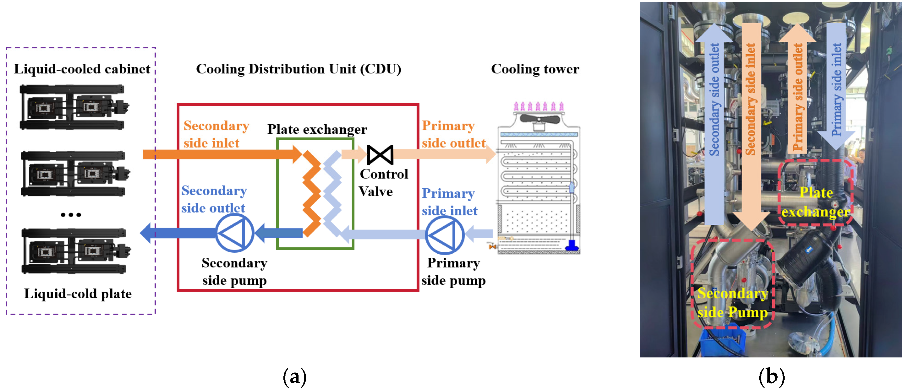
This study draws on field measurements and model development for a cold plate liquid cooling system in a data center setting. Figure 1a shows a schematic of the arrangement. The cold plate liquid cooling system consists of server racks, a coolant distribution unit (CDU) heat exchange module, and a closed-circuit cooling tower. It operates with two hydraulically isolated water loops, a primary loop and a secondary loop. In the secondary loop, a pump circulates water that collects heat absorbed at the cold plates. The warmed return flow is gathered and delivered to the CDU, where a heat exchanger transfers that heat to the primary loop. In the primary loop, the fluid, regulated by a pump and a control valve, carries the heat to the closed-circuit cooling tower and rejects it to the ambient environment. The cooled fluid then returns to the CDU at a lower temperature, providing stable cooling supply conditions to the secondary loop. In this way, the system enables efficient heat removal and temperature control for high power servers.

An experimental rig was built comprising a cold plate liquid cooled rack system, a CDU and a cooling tower. The end load of the system consisted of eight NVIDIA GB200 liquid cooled racks. Each rack has a rated power of 120 kW. Inside the racks, the chip surfaces are fitted with finned water-cooled heat sinks. Cooling water in the secondary loop removes heat through these heat sinks. Deionized water is used as the working fluid in both the primary and secondary loops. Figure 1b illustrates the internal structure of the CDU. The CDU contains a plate heat exchanger, two pumps, and a control valve, and it governs circulation in both the primary and secondary piping loops.

The testbed was instrumented with mass flow meters, temperature sensors, and pressure sensors, as detailed in

Table 1. Specifications of test instruments.

Instrument	Model	Manufacturer	City, State/Country	Operating Parameters
Server Rack	NVIDIA GB200	NVIDIA Corporation	Santa Clara, CA, USA	Rack Rated Power: 120 kW
Plate exchanger	—	—	—	Heat exchange area Ae: 13.85 m2; Heat transfer coefficient Ke: 3125 W/(m2⋅K).
Primary side Pump	CR 125	Grundfos Pumps (Shanghai) Co., Ltd.	Shanghai, China	Rated Flow Rate: 125 m3/h Liquid Temperature: 20 °C Rated Head: 85.65 m
Secondary side Pump	CR 95	Grundfos Pumps (Shanghai) Co., Ltd.	Shanghai, China	Rated Flow Rate: 94.98 m3/h Liquid Temperature: 20 °C Rated Head: 93.67 m
Primary side control Valve	Belimo SRF24A SR 5	BELIMO Automation AG	Hinwil, Switzerland	Pipe Diameter: DN150 Actuation Time: 90 s
Temperature and Humidity Data Logger	Testo 174H	Testo Instruments International Trading (Shanghai) Co., Ltd.	Shanghai, China	Temperature: −20 °C~+70 °C Relative Humidity: 0~100%RH Accuracy: ±0.5 °C, ±3% RH
Mass Flow Meter	CFMI DN150	Q&T Instrument Limited	Kaifeng, China	Temperature: 60 °C~+200 °C Measurement Range: 0~250 T/h Accuracy: ±0.1 kg/s
Pressure Sensor	WMB2780	Xi’an Shenghongchuang Instrument Co., Ltd.	Xi’an, China	Measurement Range: 0~100 MPa Accuracy: ±0.25 MPa

. The CDU control cabinet can display and record time series data from each measurement point in real time. The pumps are driven by variable frequency motors, and the cooling tower fan also uses variable frequency control to adapt to changing loads and reduce energy use. Data were collected at five-second intervals from 25 to 28 August 2025, corresponding to late-summer operating conditions. A total of 60,642 records were obtained and used as the engineering dataset for this study. Because the measurements represent a late-summer operating window rather than year-round climate conditions, the absolute values of some dynamic metrics may vary under other seasonal ambient states. For this reason, the climatic applicability of the source-side regulation pathway is further examined through the wet-bulb sensitivity analysis reported in Appendix D.

2.2. Dynamic Simulation Model

Modelica, an equation-based modelling and simulation language, is widely used to simulate heating, ventilation, and air conditioning (HVAC) systems [33,34]. Building on the existing testbed, this study develops a dynamic mathematical model in Modelica. The model comprises three main components. The first is a CDU heat exchanger model, which captures how heat transfer varies with hydraulic operating conditions on the primary and secondary sides. It is used to represent how flow rate and temperature affect both the magnitude of heat transfer and the rate at which it stabilizes. The second is a cooling tower model. By analyzing operating conditions on the primary loop, it describes how variable frequency control of the cooling tower fan influences the system’s water temperature, and it assesses the tower’s ability to respond dynamically as cooling demand changes. The third is a system delay model, designed to represent how dynamic delay parameters, including control logic latency under different strategies, equipment actuation time, and the thermal inertia of the working fluid in the piping network, shape the system’s response and controllability.

2.2.1. CDU Heat Exchanger Model

This paper uses a steady state heat exchanger model based on the effectiveness–number of transfer units method (ε–NTU) to describe heat transfer between two fluid streams [35]. The approach determines the heat exchanger effectiveness ε from the relationship between the overall heat transfer conductance $UA$ and the two streams’ heat capacity rates C, and then calculates the heat duty and outlet states. The instantaneous heat transfer rate can be expressed as:

$$\dot{Q}=\epsilon {\dot{Q}}_{\mathrm{m}\mathrm{a}\mathrm{x}}$$

(1)

Here, $\epsilon$ is the heat exchanger effectiveness, calculated using Equation (5). ${\dot{Q}}_{\mathrm{m}\mathrm{a}\mathrm{x}}$ is the maximum heat transfer rate achievable under the specified inlet conditions, calculated using Equation (4).

$$C_1={\dot{m}}_1{c}_{p,1},C_2={\dot{m}}_2{c}_{p,2}$$

(2)

$$C_{\mathrm{m}\mathrm{i}\mathrm{n}}=\min \left(C_1,C_2\right),C_{\mathrm{m}\mathrm{a}\mathrm{x}}=\max \left(C_1,C_2\right)$$

(3)

$${\dot{Q}}_{\mathrm{m}\mathrm{a}\mathrm{x}}=C_{\mathrm{m}\mathrm{i}\mathrm{n}}\left(T_{\mathrm{hot},\mathrm{in}}-T_{\mathrm{cold},\mathrm{in}}\right)$$

(4)

In these expressions, ${\dot{m}}_i$ is the mass flow rate (kg/s); $c_{p,i}$ is the specific heat at constant pressure (J/(kg·K)); $C_{\mathrm{m}\mathrm{i}\mathrm{n}}$ and $C_{\mathrm{m}\mathrm{a}\mathrm{x}}$ are the minimum and maximum heat capacity rates (J/(K·s)); $T_{\mathrm{hot},\mathrm{in}}$ is the higher of the two inlet temperatures (K); and $T_{\mathrm{cold},\mathrm{in}}$ is the lower inlet temperature (K).

$$\epsilon ={\displaystyle \frac{1-\mathrm{e}\mathrm{x}\mathrm{p}[-\mathrm{NTU}(1-Z\left)\right]}{1-Z\mathrm{e}\mathrm{x}\mathrm{p}[-\mathrm{NTU}(1-Z\left)\right]}}$$

(5)

$$\mathrm{NTU}={\displaystyle \frac{UA}{C_{\mathrm{m}\mathrm{i}\mathrm{n}}}},Z={\displaystyle \frac{C_{\mathrm{m}\mathrm{i}\mathrm{n}}}{C_{\mathrm{m}\mathrm{a}\mathrm{x}}}}$$

(6)

$${\displaystyle \frac{1}{UA}}={\displaystyle \frac{1}{h{A}_1}}+{\displaystyle \frac{1}{h{A}_2}}$$

(7)

Here, Z is the capacity ratio. $\mathrm{NTU}$ is the number of transfer units (dimensionless). $UA$ represents the overall heat transfer conductance. $h$ is the convective heat transfer coefficient (W/(m²·K)); $A_i$ is the heat transfer area on the corresponding fluid side (m²).

2.2.2. Cooling Tower Model

The cooling tower model adopts an empirical formulation based on the YorkCalc method [36]. It is used to describe how, under off design conditions, variations in water flow, air flow, and cooling water inlet temperature affect the tower’s heat rejection performance. The YorkCalc formulation in Equation (9) is an empirically derived off-design correlation that predicts the quasi-steady approach temperature—and thus, the equilibrium heat-rejection capacity—as a function of the temperature range, ambient wet-bulb temperature, and liquid-to-gas ratio. In the present work, the reported minute-scale dynamics under cooling-tower outlet temperature control are not attributed to the algebraic YorkCalc correlation alone. Instead, the overall plant is modeled dynamically in Modelica, and the dominant inertia is captured at the circulating-loop level through explicit transport delay and water thermal storage representation (Section 2.2.3). The model calculates the cooling water outlet temperature, $T_{cw}$, using the approach temperature $T_{App}$:

$$T_{cw}=T_{App}+T_{wb}$$

(8)

In this expression, $T_{wb}$ is the outdoor wet bulb temperature (K). The approach temperature $T_{App}$ is treated as a function of the tower’s inlet–outlet temperature difference, the outdoor wet bulb temperature, and the liquid to gas ratio, and is calculated as follows:

$$\begin{array}{cc}\hfill T_{App}=g_1+g_2{T}_{wb}& +g_3{T}_{wb}^2+g_4{T}_r+g_5{T}_{wb}{T}_r+g_6{T}_{wb}^2{T}_r+g_7{T}_r^2+g_8{T}_{wb}{T}_r^2\hfill \\ & +g_9{T}_r^2{T}_r^2+g_{10}Lgr+g_{11}{T}_{wb}Lgr+g_{12}{T}_{wb}^{2}Lgr+g_{13}{T}_{r}Lgr\hfill \\ & +g_{14}{T}_{wb}{T}_{r}Lgr+g_{15}{T}_r^{2}Lgr+g_{16}{T}_{wb}{T}_r^{2}Lgr+g_{17}{T}_{wb}^2{T}_r^{2}Lgr\hfill \\ & +g_{18}{T}_r^2{T}_r^{2}Lgr+g_{19}Lg{r}^2+g_{20}{T}_{wb}Lg{r}^2+g_{21}{T}_{wb}^{2}Lg{r}^2\hfill \\ & +g_{22}{T}_{r}Lg{r}^2+g_{23}{T}_{wb}{T}_{r}Lg{r}^2+g_{24}{T}_r^2{T}_{r}Lg{r}^2+g_{25}{T}_r^{2}Lg{r}^2\hfill \\ & +g_{26}{T}_{wb}{T}_r^{2}Lg{r}^2+g_{27}{T}_{wb}^2{T}_r^{2}Lg{r}^2\hfill \end{array}$$

(9)

Here, $T_r$ is the inlet–outlet temperature difference (K); $[g_1,g_2,\dots ,g_{27}]$ are polynomial coefficients; and the liquid to gas ratio $Lgr$ is defined as the ratio of water flow to air flow:

$$Lgr={\displaystyle \frac{m_{wat,ac}/m_{wat,no}}{m_{air,ac}/m_{air,no}}}$$

(10)

In these terms, $m_{wat,ac}$ is the current cooling water mass flow rate (kg/s); $m_{wat,no}$ is the nominal cooling water mass flow rate (kg/s); $m_{air,ac}$ is the current air mass flow rate (kg/s); and $m_{air,no}$ is the nominal air mass flow rate (kg/s).

2.2.3. System Delay Model

This study uses the DelayFirstOrder model [37] to represent the transport delay effect caused by the fluid’s thermal inertia. The model implements a fully mixed lumped volume in the form of a MixingVolume. It then calculates an equivalent volume automatically from the nominal mass flow rate $m_{\mathrm{flow}\text{\_}\mathrm{no}}$ and a specified time constant $\tau$, ensuring that, under nominal operating conditions, the medium’s mean residence time in that volume matches the intended delay. The dynamic process is described by Equation (11), and the corresponding hold (waiting) process is given by Equation (12).

$$\left\{\begin{array}{c}{\displaystyle \frac{dm\left(t\right)}{dt}}={\displaystyle \sum _{i=1}^N}{m}_i\left(t\right)\\ {\displaystyle \frac{dU\left(t\right)}{dt}}={\displaystyle \sum _{i=1}^N}{m}_i\left(t\right)h_i\left(t\right)+Q\left(t\right)\end{array}\right.$$

(11)

$$\left\{\begin{array}{c}0={\displaystyle \sum _{i=1}^N}{m}_i\left(t\right)\\ 0={\displaystyle \sum _{i=1}^N}{m}_i\left(t\right)h_i\left(t\right)+Q\left(t\right)\end{array}\right.$$

(12)

In these equations, $m_i$ is the inlet mass flow rate (kg/s); $U$ is internal energy (kJ); $h_i$ is specific enthalpy (kJ/kg); and $Q$ is the externally imposed heat flow rate (kW).

As shown in Equation (13), within the equipment model the mass term in Equation (11) is replaced by the product of the time constant and the nominal flow rate. This is used to describe the dynamics of a first order delay.

$$m=\tau \cdot m_{\mathrm{flow}\text{\_}\mathrm{no}}$$

(13)

Here, $\tau$ is the time constant, and $m_{\mathrm{flow}\text{\_}\mathrm{no}}$ is the nominal mass flow rate (kg/s).

The methodological contribution of the present delay treatment does not lie in the invention of the DelayFirstOrder model itself, but in its physically interpretable integration into a dual-loop liquid-cooled data-center plant. Compared with a delay-free lumped formulation, the adopted approach avoids unrealistically instantaneous temperature propagation along the circulation loop. Compared with a pure dead-time block, it better preserves the progressive attenuation and mixing behavior caused by water-side transport and thermal capacitance, while remaining numerically convenient for integration with the coupled Modelica energy-balance framework. Therefore, the contribution of the present delay treatment lies in linking plant-level transport smoothing to actuator-pathway comparison and coordinated control screening in liquid-cooled data-center operation, rather than in introducing a new generic delay model.

2.2.4. Simulation Model Validation Metrics

In this study, we quantify the agreement between the simulation outputs and the measured data by characterizing both the overall error level and the worst-case deviation. The root mean square error (RMSE) and the mean absolute error (MAE) are used to represent the global discrepancy, whereas the maximum absolute error (Max error) is reported to capture the deviation under the most unfavorable condition. To enable comparisons across variables with different units and scales, we further introduce the normalized root mean square error (NRMSE), computed by normalizing the RMSE with the range of the measured values. In addition, to assess potential systematic overestimation or underestimation, we report the normalized mean bias error (NMBE). Taken together, these metrics provide a comprehensive evaluation of model fidelity, including the overall fit and the peak error characteristics.

$$\mathrm{R}\mathrm{M}\mathrm{S}\mathrm{E}=\sqrt{{\displaystyle \frac{1}{n}}{\displaystyle \sum _{i=1}^n} {\left({\widehat{y}}_i-y_i\right)}^2}$$

(14)

$$\mathrm{M}\mathrm{A}\mathrm{E}={\displaystyle \frac{1}{n}}{\displaystyle \sum _{i=1}^n} |{\widehat{y}}_i-y_i|$$

(15)

$$\mathrm{M}\mathrm{a}\mathrm{x} \mathrm{e}\mathrm{r}\mathrm{r}\mathrm{o}\mathrm{r}=\underset{1\le i\le n}{max} |{\widehat{y}}_i-y_i|$$

(16)

$$\mathrm{N}\mathrm{R}\mathrm{M}\mathrm{S}\mathrm{E}(\%)={\displaystyle \frac{\mathrm{R}\mathrm{M}\mathrm{S}\mathrm{E}}{\max \left(y\right)-\mathrm{m}\mathrm{i}\mathrm{n}\left(y\right)}}\times 100\%$$

(17)

$$\mathrm{N}\mathrm{M}\mathrm{B}\mathrm{E}(\%)={\displaystyle \frac{\sum _{i=1}^n ({\widehat{y}}_i-y_i)}{\frac{\left(n-1\right)}{n}\sum _{i=1}^n y_i}}\times 100\%$$

(18)

Here, n denotes the number of samples, $y_i$ is the measured value at sample i, and ${\widehat{y}}_i$ is the corresponding simulated value. In this work, the NRMSE is computed by normalizing the RMSE with the range of the measured values, and both the NRMSE and the NMBE are reported in percentage form. In selecting the validation metrics, we also considered other commonly used indicators such as R², MAPE, and CVRMSE. However, the present validation task is a transient step-response problem rather than a long-horizon steady prediction problem. For this reason, R² was not used as a primary metric because it may remain high even when transient timing mismatch and turning-point deviation are still significant. MAPE was also not adopted because the temperature variation range in some stages is narrow, making percentage errors sensitive to small denominators and less interpretable for transient thermal responses. CVRMSE was not reported separately because, for the present purpose, it provides information largely similar to NRMSE after scale normalization. We, therefore, retained RMSE, MAE, NRMSE, NMBE, and maximum error as the primary indicators, since together they capture overall discrepancy, scale-normalized deviation, systematic bias, and worst-case transient error. In addition, agreement in trend direction and major turning points was used as a supplementary qualitative check of dynamic fidelity.

2.2.5. Control-Theoretic Abstraction of Actuator Pathways

To complement the engineering observations with a control-theoretic interpretation, the coupled hydraulic–thermal plant is locally abstracted around a representative operating condition. A classical and practically interpretable way to describe delay-dominant thermal processes is to use a low-order state-space representation together with an equivalent first-order-plus-dead-time (FOPDT) reduction, which has been widely adopted in process control and forms the basis of SIMC-type tuning rules [24]. In the present study, the manipulated variables are the primary-side valve opening, the primary-side pump actuation, and the cooling-tower fan actuation, while the controlled output is the secondary-side supply temperature. The local linearized form is written as:

$$\dot{\mathrm{x}}=\mathrm{A}\delta \mathrm{x}+\mathrm{B}\delta \mathrm{u},\delta \mathrm{y}=\mathrm{C}\delta \mathrm{x}+\mathrm{D}\delta \mathrm{u}$$

(19)

$$\begin{array}{c}x=[T_{p,in},T_{p,out},T_{s,in},T_{s,out},m_p,T_{ct,out}{]}^T,\\ u=[{\alpha }_v,n_p,n_f{]}^T,\\ y=T_{s,in}\end{array}$$

(20)

Here, $T_{p,in}$ and $T_{p,out}$ denote the primary-side inlet and outlet temperatures, $T_{s,in}$ and $T_{s,out}$ denote the secondary-side supply and return temperatures, $m_p$ is the primary-side mass flow rate, ${\alpha }_v$ is the valve opening, $n_p$ is the pump actuation, and $n_f$ is the cooling-tower fan actuation.

For pathway-level interpretation and cross-strategy comparison, each actuator-to-output channel is further reduced to an equivalent FOPDT model.

$$G_i(s)={\displaystyle \frac{K_i{e}^{-{\theta }_{i}s}}{{\tau }_{i}s+1}}$$

(21)

where $K_i$, ${\theta }_i$, and ${\tau }_i$ denote the pathway gain, effective delay, and dominant time constant, respectively. In this study, the FOPDT parameters are identified from the 0.4-step responses of the three single-actuator strategies using the secondary-side supply temperature time series. The command trigger time is fixed at t = 100 s. The value at t = 100 s is taken as the baseline output y₀, and the final sampled value is taken as the steady-state output y_∞. The effective delay ${\theta }_i$ is defined as the elapsed time required for the output to first reach 2% of the total change, while the dominant time constant ${\tau }_i$ is determined from the 63.2% crossing of the total change after removing the delay term. This reduced-order representation is used here as an explanatory model rather than a high-precision predictive surrogate, with the aim of clarifying why the three manipulated variables exhibit markedly different transient behaviors in terms of response speed, fluctuation tendency, and delay-related control difficulty.

2.3. Performance Indicator

The control logic in the Modelica simulation mirrors that of the real installation. The control valve, pumps, and cooling tower components respond to changes in the end load by adjusting operating conditions, with the aim of keeping server inlet temperature constant. To ensure that comparisons among control strategies are made on a consistent basis, this study uses step changes to adjust component operating conditions. It defines the change in a manipulated variable across a component’s operating range as the component’s step magnitude. Let the manipulated variable for a given control strategy be $u\left(t\right)$. Depending on the strategy, this may represent valve opening, primary side pump flow rate, or cooling tower fan frequency. Using the component’s maximum manipulated value $u_{\mathrm{m}\mathrm{a}\mathrm{x}}$ as the normalisation reference, when a step disturbance of magnitude $p$ is applied, the post step target value is defined as:

$$u_{\mathrm{t}\mathrm{a}\mathrm{r}}=u\left(t_0\right)+p\cdot u_{\mathrm{m}\mathrm{a}\mathrm{x}}$$

(22)

where $u_{\mathrm{t}\mathrm{a}\mathrm{r}}$ is the target manipulated value after the step, such as target valve opening, target pump flow rate, or target fan frequency; and $t_0$ is the time at which the control command is issued. In this study, the step magnitude $p$ is set in increments of 0.1.

To keep the initial operating point stable, the command issuance time is fixed at $t_0=100$ s for all simulated cases. To standardise the reference across parameters, this study defines the cooling system variable as stable once the observed parameter reaches 99.6% of its total change. Because GB200 full cabinets are substantially more expensive than conventional server cabinets, operational risk considerations require higher stability of the cabinet supply liquid temperature. Accordingly, this study adopts a conservative stability threshold for the settling criterion.

Table A1. The stable schedule of cooling capacity under different strategies.

Control Strategy	Step	95%	98%	99%	99.6%
Cooling Tower Outlet Temperature Control	0.2	373.9	503.3	600.2	721.8
	0.4	404	542.1	644.8	775.7
	0.6	423.8	567.6	674.2	811.3
Constant Differential Pressure Valve Control	0.2	40.6	40.6	40.7	40.7
	0.4	41.1	41.1	41.2	41.2
	0.6	41.2	41.3	41.3	41.3
Variable Flow Pump Control	0.2	52.4	54.5	55.4	56.2
	0.4	68.1	68.7	68.9	69
	0.6	71.1	72.2	72.6	72.9

and

Table A2. The stable schedule of the secondary-side supply temperature under different strategies.

Control Strategy	Step	95%	98%	99%	99.6%
Cooling Tower Outlet Temperature Control	0.2	374.2	503.5	600.6	722.2
	0.4	404.3	542.3	644.9	775.8
	0.6	424	567.9	674.4	811.6
Constant Differential Pressure Valve Control	0.2	40.7	40.8	40.8	40.8
	0.4	41.3	41.3	41.4	41.4
	0.6	41.4	41.5	41.5	41.5
Variable Flow Pump Control	0.2	52.6	54.7	55.6	56.4
	0.4	68.3	68.9	69.1	69.2
	0.6	71.3	72.4	72.8	73.1

further show that using a stricter stability threshold does not affect the subsequent conclusions, as the comparative trends and relative performance among strategies remain unchanged. Equivalently, when the system first satisfies Equation (23), it is deemed to have reached a new steady state, and the first time at which Equation (23) is satisfied is defined as the stabilization time $t_{\mathrm{s}\mathrm{t}\mathrm{a}\mathrm{b}\mathrm{l}\mathrm{e}}$.

$$|x(t)-x_{\mathrm{\infty }}|\le 0.004\cdot |\Delta x|$$

(23)

$$\Delta x=x_{\mathrm{\infty }}-x_0, x_{\mathrm{\infty }}=x\left(t_{\mathrm{e}\mathrm{n}\mathrm{d}}\right), x_0=x\left(t_0\right)$$

(24)

where $x_0$ is the baseline value of the system parameter before the step at $t_0=100 \mathrm{s}$; $x_{\mathrm{\infty }}$ is the post step steady state value; $t_{end}$ is the final time of the simulation; and $\Delta x$ is the change in the cooling system parameter.

For dynamic performance evaluation, the paper introduces the dynamic response time $t_{\mathrm{r}\mathrm{e}\mathrm{s}\mathrm{p}}$ as the stabilisation time metric. It is used to characterise how long the system takes, after a control command is triggered, to regulate the parameter to its new steady state.

$$t_{\mathrm{r}\mathrm{e}\mathrm{s}\mathrm{p}}=t_{\mathrm{s}\mathrm{t}\mathrm{a}\mathrm{b}\mathrm{l}\mathrm{e}}-t_0$$

(25)

The transient swings in system variables during component adjustment can materially affect the operational risk of liquid cooled servers. To capture this, we introduce two measures: the dynamic fluctuation amplitude $\Delta x_{\mathrm{e}\mathrm{x}\mathrm{t}}$ and the dynamic fluctuation ratio ${\eta }_x$. The former describes the maximum departure of a system variable from its final steady state during the transient. The latter is intended to remove differences in steady state magnitude across operating conditions, making it easier to compare the fluctuation risk of different control strategies on a like for like basis.

In this study, the dynamic fluctuation amplitude is defined as the difference between the extreme value reached during the transient and the final steady state value:

$$\Delta x_{\mathrm{e}\mathrm{x}\mathrm{t}}=\left\{\begin{array}{c}{x}_{max}-x_{\mathrm{\infty }}, \Delta x\ge 0\\ x_{\mathrm{\infty }}-x_{min}, \Delta x<0\end{array}\right.$$

(26)

$$x_{max}=\underset{t\ge t_0}{max} x\left(t\right),x_{min}=\underset{t\ge t_0}{min} x(t)$$

(27)

where $\Delta x$ is the change in the system variable. If $\Delta x\ge 0$, the potential risk takes the form of overshoot, and the extreme is the maximum value $x_{max}$. If $\Delta x<0$, the potential risk takes the form of undershoot, and the extreme is the minimum value $x_{min}$.

The dynamic fluctuation ratio ${\eta }_x$ is then defined as the ratio of the dynamic fluctuation amplitude to the final steady state value, as shown in Equation (28). It is a dimensionless indicator. Smaller values indicate a smoother transient and a lower risk of overshoot or undershoot.

$${\eta }_x={\displaystyle \frac{\Delta x_{\mathrm{e}\mathrm{x}\mathrm{t}}}{x_{\mathrm{\infty }}}}$$

(28)

2.4. Simulation Methods and Operating Condition Design

2.4.1. Simulation Model and Validation

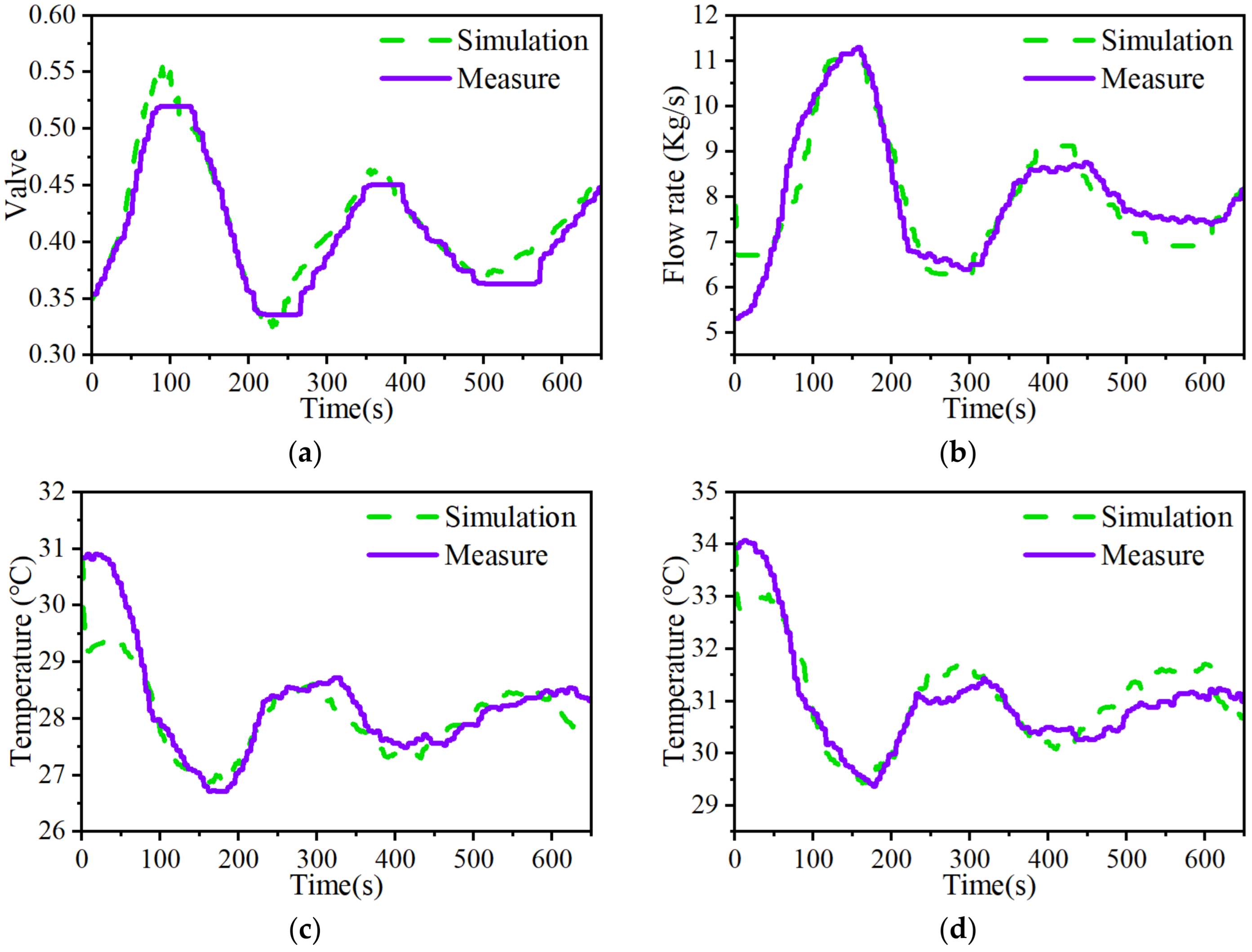
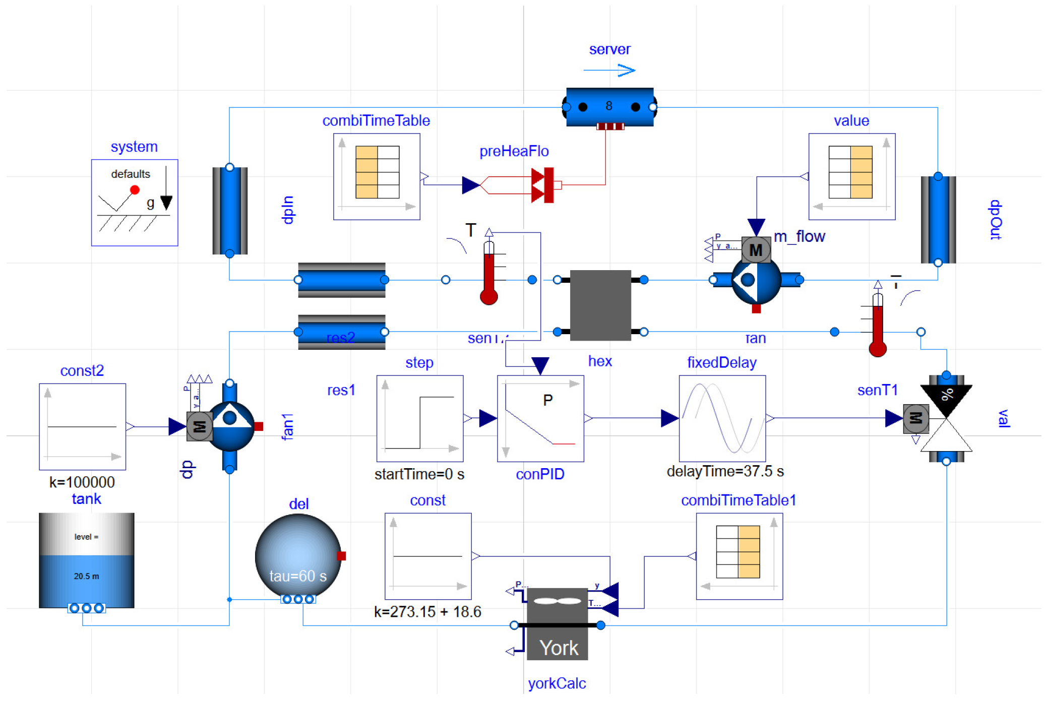
Because field conditions allow only a limited amount of experimental data, the study relies on a dynamic liquid cooling simulation model, built in Modelica on the established simulation platform, to refine and analyze system behavior across a wide range of combined operating conditions and thereby optimize dynamic response time and steady state accuracy. The model, shown in Figure 2, is validated using a typical setpoint step event that can be implemented on site. After the terminal server load is held constant and the system has reached steady operation, the secondary side outlet water temperature setpoint is changed from 30 °C to 28 °C. The system then adjusts primary side flow in response to the altered cooling demand, and the time series responses of key cooling system variables are recorded for comparison. By examining the agreement between simulated and measured temperature response trends, as well as the distribution of errors, the study confirms that the model can reproduce the dominant dynamic features under load disturbances and control actions within an acceptable error range.

2.4.2. Step Response Simulations for Single Manipulated Variable Strategies

The primary and secondary circuits are hydraulically decoupled and interact only through the CDU plate heat exchanger, whereas the CDU internal pumps and control valve sustain circulation on both sides. Accordingly, the lower-level loop considered in this study actuates the primary side and treats the secondary side pump and valve dynamics as a fast local boundary condition. In the step tests, the secondary side return temperature and flow are held fixed, and the primary-side flow is adjusted to satisfy changes in the secondary side temperature setpoint.

To ensure cooling supply can follow changes in end load, the system can adopt different regulation strategies. Primary side flow can be adjusted by changing valve opening or by varying pump speed, while primary side water temperature can be regulated by varying cooling tower fan speed. This leads to three single manipulated variable strategies: constant differential pressure valve control, variable flow pump control, and cooling tower outlet temperature control. The study conducts step response simulations for all three, to characterize the dynamics of single component actuation.

• Constant differential pressure valve control: In engineering practice, this strategy corresponds to operating the primary side pump under constant differential pressure and regulating flow by adjusting the primary side control valve opening. The test conditions fix the secondary side CDU return water temperature and flow. The cooling tower fan is switched off so that the tower operates under natural convection. Outdoor conditions are set to 25 °C and 60% relative humidity. The primary side pump runs under constant differential pressure, with the setpoint equal to its rated head. Valve opening is stepped upward in 10% increments across a range of 30% to 100%. Starting from 30% opening, the step magnitude is taken from 0.1 to 0.7.
• Variable flow pump control: This strategy varies the speed of the primary side pump to change primary side flow and quickly regulate heat transfer. The test conditions again fix the secondary side CDU return water temperature and flow. The cooling tower fan remains off, and the tower operates under natural convection, with outdoor conditions set to 25 °C and 60% relative humidity. To remove the influence of changes in local valve resistance, the primary side valve is held fully open at 100%. The primary side pump frequency is stepped upward from a 20 Hz baseline, in 5 Hz increments. The step magnitude ranges from 0.1 to 0.6, corresponding to frequency increases from 5 Hz to 30 Hz.
• Cooling tower outlet temperature control: This strategy changes the heat exchange intensity on the tower side by adjusting cooling tower fan frequency. In doing so, it alters the cooling plant outlet water temperature and regulates cooling capacity. The test conditions fix the secondary side CDU return water temperature and flow. The primary side valve remains fully open at 100%. The primary side pump operates at constant flow, holding system flow at 35 kg/s. Outdoor conditions are set to 25 °C and 60% relative humidity. The cooling tower fan frequency is stepped upward from an initial value of 15 Hz. The step magnitude ranges from 0.1 to 0.7, corresponding to increases of 5 Hz to 35 Hz.

2.4.3. Positive and Negative Step Response Simulations

In real world operation, data center IT loads fluctuate in both directions. A surge in demand may require cooling capacity to rise quickly, while a drop in load calls for timely reductions in cooling output. To characterize the dynamics when cooling demand falls, and to test whether the dynamic evaluation framework developed in this paper remains applicable and comparable when the step direction is reversed, the study conducts negative step tests for the variable flow pump strategy and the cooling tower outlet temperature strategy. The negative steps use exactly the same trigger time and stability criterion as the positive steps, ensuring that the two sets of results can be compared directly.

2.4.4. Step Response Simulations for Combined Operating Conditions

To move beyond the inherent limitations of a single manipulated variable, which often forces a tradeoff between response speed and fluctuation risk, the study adopts a combined regulation strategy that pairs primary side variable flow pumping with variable frequency control of the cooling tower fan. A match and screen operating condition library is then constructed in a two-dimensional operating space. The combined scan is performed on a regular grid. Cooling tower fan frequency starts at 15 Hz and increases in 5 Hz increments to 50 Hz, while primary side pump flow starts at 20 kg/s and increases in 5 kg/s increments to 50 kg/s. This yields 56 operating conditions in total. Batch steady state simulations are run for each condition to obtain a mapping of system cooling capacity.

Building on this steady state cooling capacity map, the study embeds the dynamic performance metrics into the combined condition database. Specifically, it selects the same representative set of load changes used in the positive and negative step analyses of the single strategies and keeps the command trigger time and stability criterion unchanged. For every combined operating point in the database, it then runs step disturbance simulations and records steady state cooling capacity together with dynamic response time, dynamic fluctuation amplitude, and the dynamic fluctuation ratio, producing a dynamic characteristics space that can be used for screening.

For operating point selection and optimization, the study uses a constraint-based approach to ensure engineering feasibility. It first sets an upper bound on acceptable fluctuation risk, treating a dynamic fluctuation ratio of no more than 5% as a hard constraint to filter out operating points with high overshoot or undershoot risk [38]. We introduce the 5% dynamic fluctuation ratio as a dimensionless stability constraint to ensure portability across liquid-cooling deployments with different coolant supply temperature setpoints, and Appendix B provides a threshold sensitivity study showing the selected optimal operating point remains consistent under reasonable variations around 5%. Subject to this constraint, it minimizes dynamic response time, selecting from the feasible combined operating conditions the operating point with the shortest stabilization time as the optimum. The final output is the corresponding pair of step magnitudes for the pump and the cooling tower fan, recommended as the combined manipulated variable setting. In effect, this provides a mapping from a target cooling demand change to an actionable combination of control inputs across the operating space.

3. Results

3.1. Case Study and Model Validation

In this study, we validate the simulation model using the constant differential pressure valve control strategy employed in the field. To assess the accuracy of the simulated hydraulic behavior, we compare the predicted and measured valve opening and flow rate dynamics. To evaluate the thermodynamic fidelity of the model, we further examine the agreement in secondary-side supply temperature and primary-side return temperature. As Figure 3 shows, the largest absolute error in secondary side supply temperature occurs early in the simulation, at t = 8 s, at about 1.71 °C. The largest absolute error in Primary side Return Water Temperature appears at t = 10 s, at about 1.31 °C. This suggests that the peak errors are concentrated in the initial transition period, a phase that is typically sensitive to the choice of initial conditions and to short lived mismatches in the transient behavior of pipework thermal inertia and the control loop before the two are fully aligned. Once the system moves into the subsequent regulation stage, the simulated and measured curves follow the same overall trend. The direction of temperature/flow rate change and the main turning points line up well.

As shown in

Table 2. This is a table of simulation model validation metrics.

Dataset Time	Metric	Valve Opening	Flow Rate	Secondary Side Supply Temperature	Primary Side Return Temperature
0–655 s	RMSE	0.02	0.51	0.48	0.44
	NRMSE	8.20%	8.55%	11.49%	9.39%
	NMBE	2.20%	−0.77%	−0.74%	0.23%
	MAE	0.01	0.39	0.32	0.35
	Max error	0.04	2.50	1.71	1.31
100–655 s	RMSE	0.01	0.37	0.26	0.35
	NRMSE	7.29%	7.59%	13.14%	17.21%
	NMBE	1.85%	−1.02%	−0.34%	0.49%
	MAE	0.01	0.31	0.21	0.30
	Max error	0.04	0.88	0.68	0.68

, over the full interval from 0 s to 655 s, the maximum temperature errors are 1.71 °C for the secondary-side supply temperature and 1.31 °C for the primary-side return temperature, while the maximum error in primary-side flow rate is 2.50. However, after excluding the start-up transient from 0 s to 100 s and evaluating only the interval from 100 s to 655 s, the peak errors decrease markedly. The flow-rate maximum error decreases from 2.50 to 0.88, corresponding to an approximately 64.8% reduction. The maximum error in secondary-side supply temperature decreases from 1.71 °C to 0.68 °C, a reduction of about 60.2%, and the maximum error in primary-side return temperature decreases from 1.31 °C to 0.68 °C, a reduction of about 48.1%. Consistent improvements are also observed in RMSE, which decreases from 0.02 to 0.01 for valve opening, from 0.51 to 0.37 for flow rate, from 0.48 to 0.26 for secondary-side supply temperature, and from 0.44 to 0.35 for primary-side return temperature. Across both intervals, the NMBE remains within a narrow range of approximately minus 1 percent to 2 percent, indicating negligible systematic bias. Overall, the model reproduces the temporal trends and key turning points with good fidelity, which is sufficient to support subsequent dynamic reproduction and comparative evaluation of control strategies. The present validation is, therefore, intended to support plant-level assessment of secondary-side supply temperature dynamics and control-strategy comparison.

Based on this evidence, and to prevent the start-up transient from disproportionately inflating dynamic fluctuation metrics such as fluctuation amplitude, fluctuation ratio, and settling criteria, we consistently use the system state at t equals 100 s as the initial reference for dynamic metric computation. In addition, both error statistics and strategy comparisons are performed using only the response segment with t greater than or equal to 100 s. This approach retains the dominant dynamic characteristics while avoiding short-duration start-up artifacts, thereby improving comparability and robustness across control strategies.

3.2. Analysis of Single Component Control Strategies

3.2.1. Constant Differential Pressure Valve Control

Under the constant differential pressure valve control strategy, valve opening is the manipulated variable, and changes in flow are used to follow shifts in cooling demand. Figure 4a shows that as the valve opening step magnitude increases from 0.1 to 0.7, primary side flow rises from 20.9 kg/s to 51.8 kg/s, and steady state cooling capacity increases from 992.4 kW to 1233.8 kW. In other words, greater primary side flow delivers more cooling. Figure 4b, however, shows that the secondary side supply temperature increases as the valve step becomes larger. The higher primary side flow leaves insufficient time for heat rejection on the cooling tower side, raising the primary side outlet temperature and, in turn, lifting the secondary side water temperature. Figure 4a also indicates diminishing marginal gains. As the step magnitude continues to rise, flow still increases, but the steady state improvement in cooling capacity begins to level off.

The strategy’s transient behavior is marked by speed, but also by pronounced volatility. After a valve step, cooling capacity exhibits a clear overshoot and then slowly settles back to its final steady state. The overshoot grows sharply with step size. With a step magnitude of 0.1, the cooling capacity overshoot is about 91.6 kW, corresponding to a dynamic fluctuation ratio of 9.2%. With a step magnitude of 0.7, the overshoot climbs to about 476.9 kW and the dynamic fluctuation ratio increases to 38.7%. This indicates that although valve control can quickly establish a new heat transfer condition, large valve openings induces larger transient deviation in cooling capacity (and associated supply temperature disturbance).

3.2.2. Variable Flow Pump Control

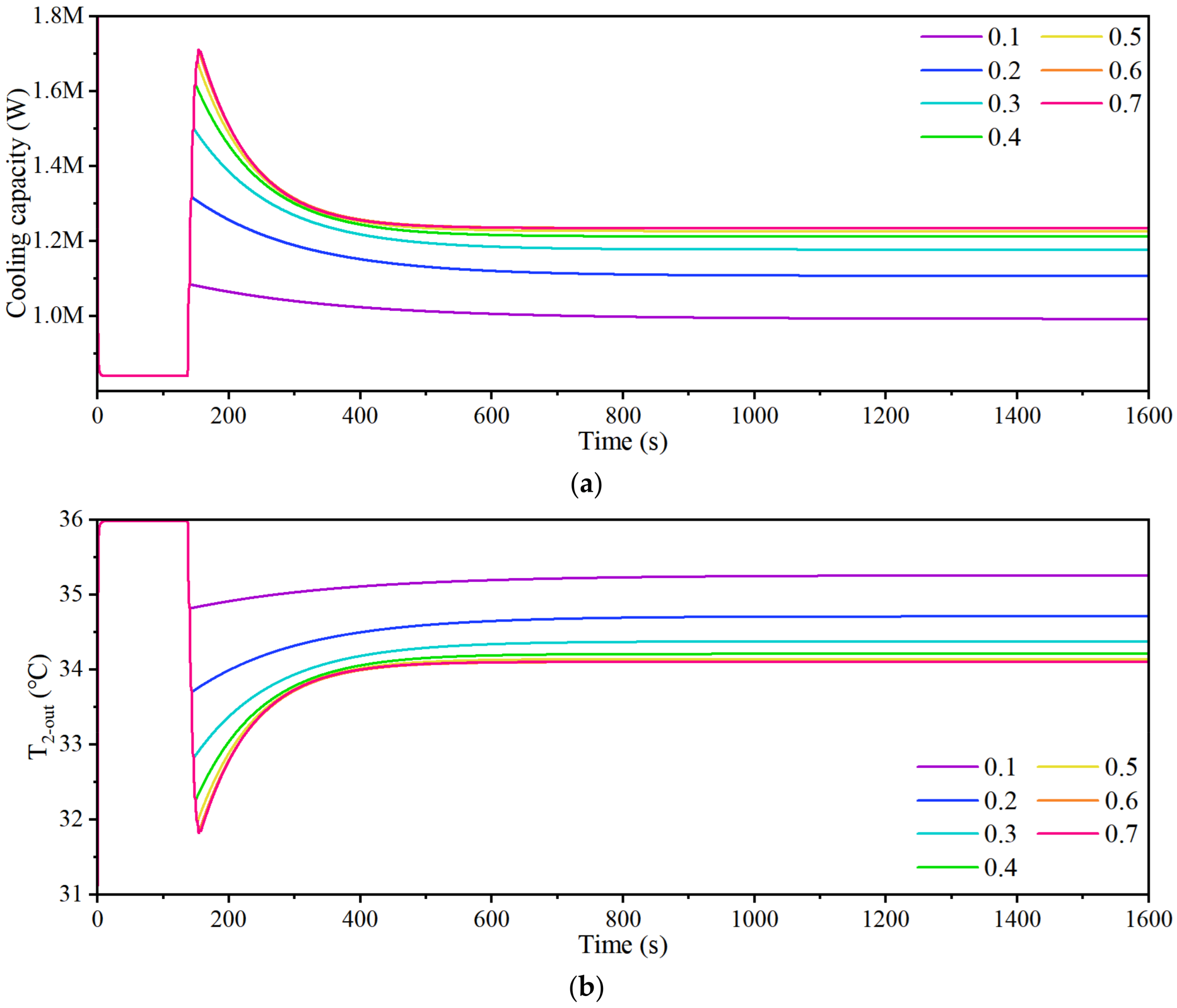
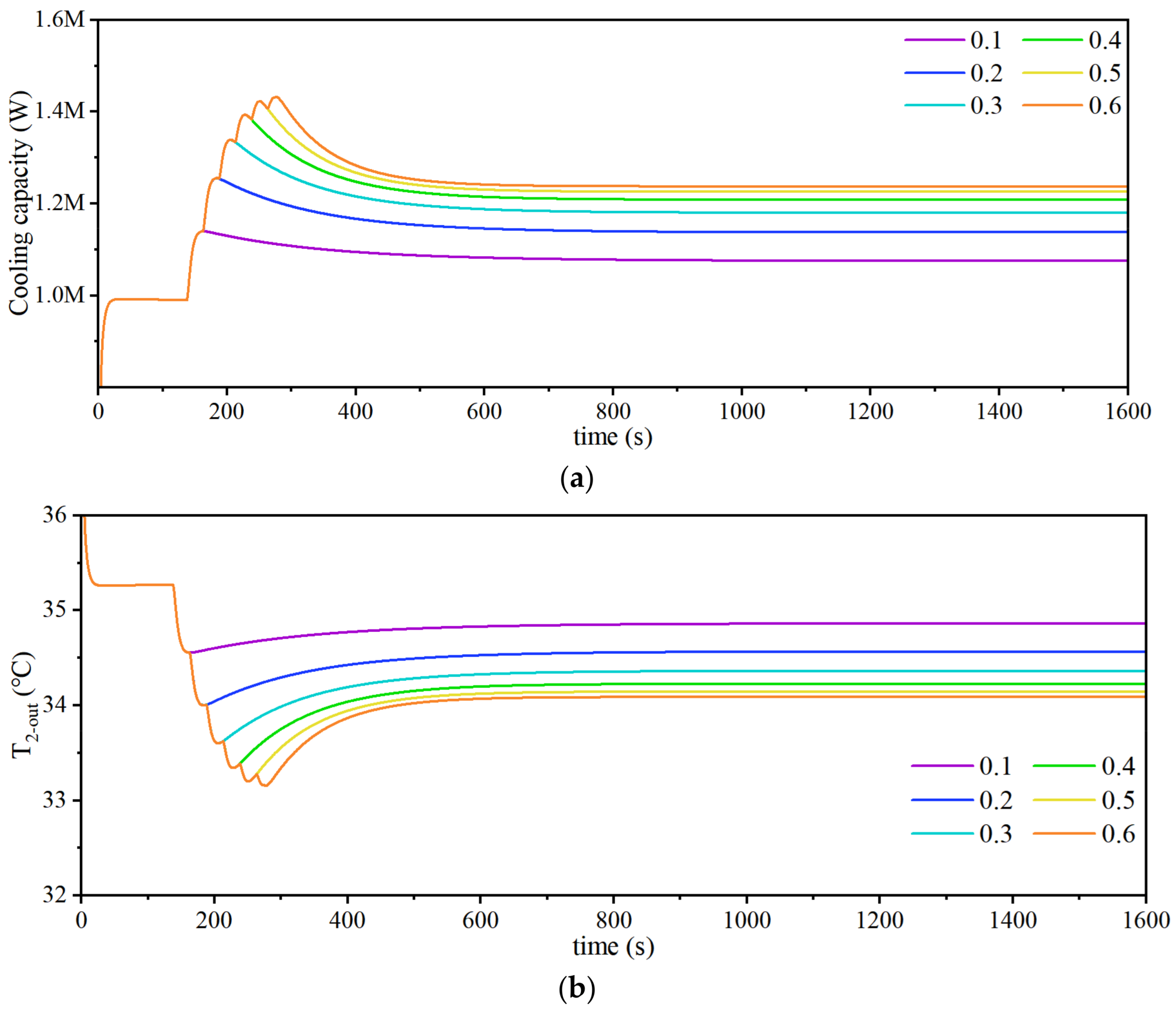
Under the variable flow pump control strategy, pump speed is the manipulated variable. This produces a more nearly linear increase in primary side flow, and the thermal response is smoother. At the same time, stabilization time lengthens noticeably as the step becomes larger. As Figure 5a shows, when the step magnitude increases from 0.1 to 0.6, primary side flow rises from 25 kg/s to 50 kg/s, and steady state cooling capacity increases from 1075.1 kW to 1237.1 kW. Like the constant differential pressure valve strategy, this approach raises cooling output by increasing flow. Compared with valve control, however, the cooling capacity gain is less sensitive to changes in flow. It also shows the same pattern of diminishing marginal returns as flow increases.

On the temperature side, Figure 5b indicates a monotonic decline in secondary side supply temperature as the step grows. The steady state value falls from 34.9 °C to 34.1 °C, although the overall decrease is smaller than under the cooling tower outlet temperature strategy. In dynamic terms, overshoot is still present, but it is markedly weaker than with valve control. At the largest step of 0.6, the cooling capacity overshoot is 195 kW, corresponding to a dynamic fluctuation ratio of about 15.8%.

3.2.3. Cooling Tower Outlet Temperature Control

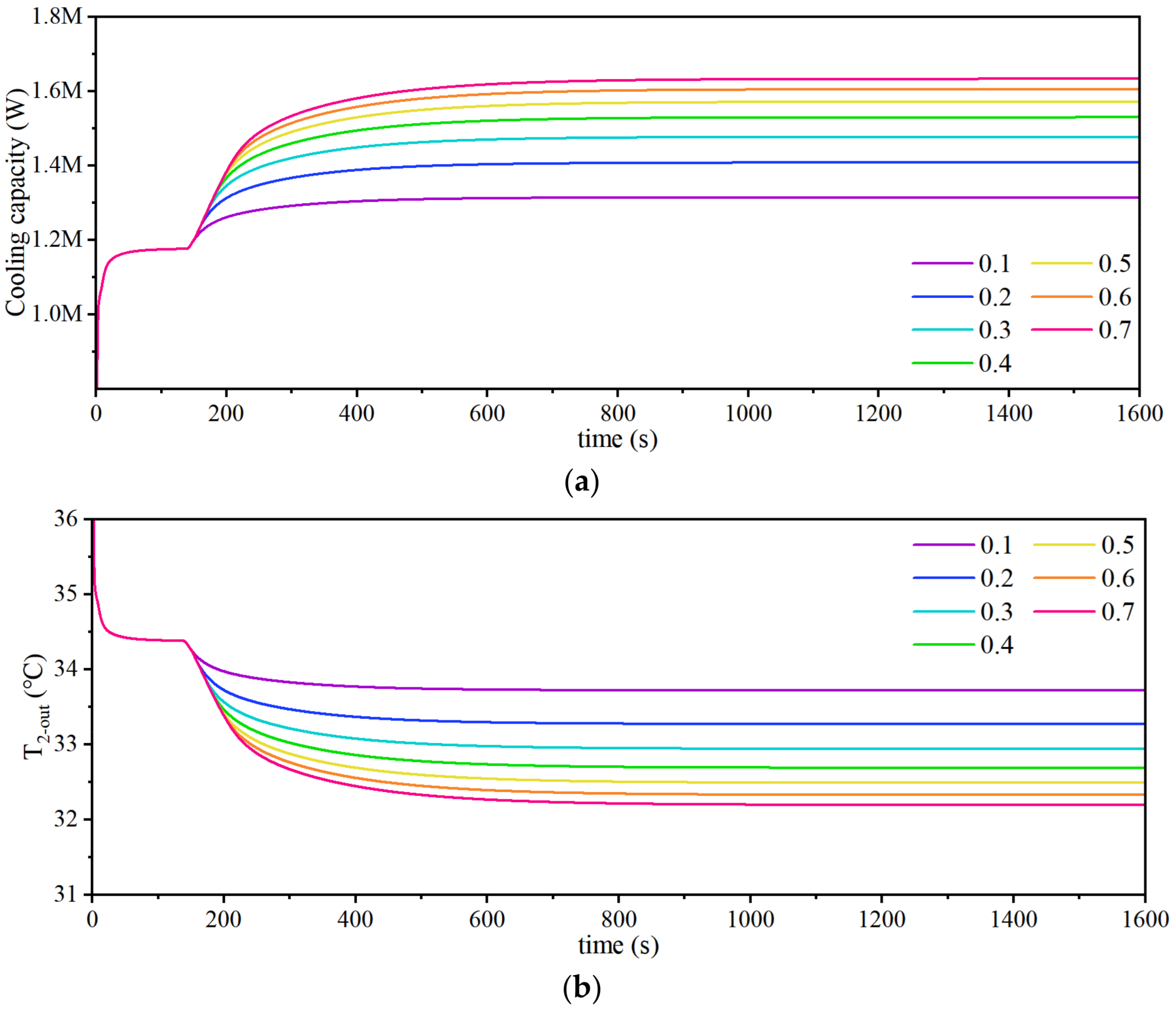
Under the cooling tower outlet temperature control strategy, cooling tower fan setting is the manipulated variable. By strengthening heat rejection on the tower side, the strategy lowers the cooling tower outlet water temperature and thereby increases the system’s cooling capacity. Its signature is clear. Cooling output and secondary side supply temperature improve markedly, overshoot is essentially absent, but the response is extremely slow. As Figure 6 shows, when the step magnitude increases from 0.1 to 0.7, the steady state cooling tower outlet temperature falls from 24.8 °C to 21.2 °C. Over the same range, system cooling capacity rises from 1314.1 kW to 1632.9 kW, while secondary side supply temperature drops from 33.7 °C to 32.2 °C. The cooling capacity response curve is almost monotonic, with overshoot negligible. The maximum overshoot is only 6.6 kW.

3.2.4. Cross-Strategy Analysis

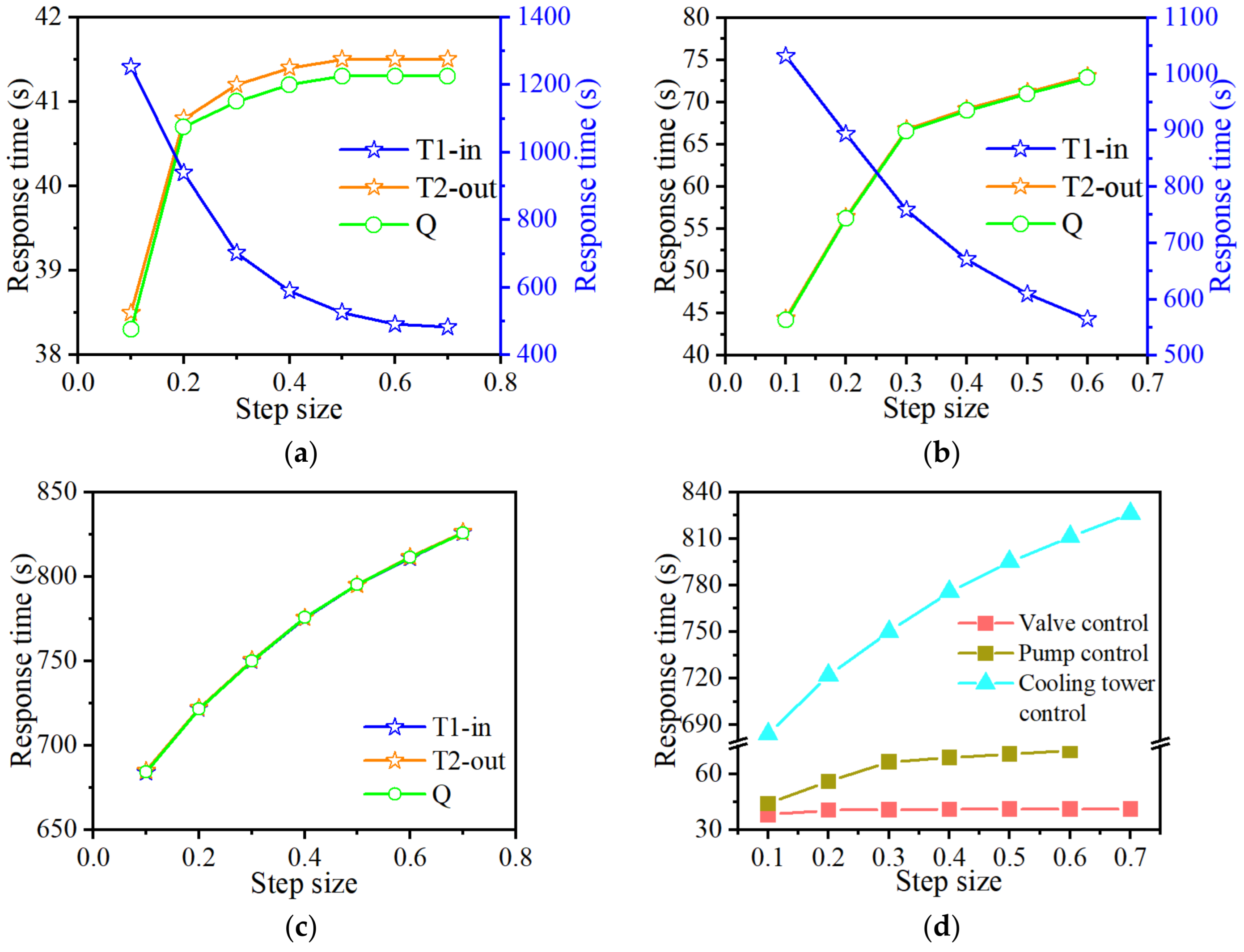
Figure 7a further shows that under positive steps, the strategy’s dynamic response time remains essentially steady at 38.3–41.3 s. It increases only slightly with step magnitude and then saturates. Yet the overshoot in cooling capacity rises markedly as the step becomes larger. Even with overshoot, the response time is very short and relatively insensitive to the step. It increases from 38.3 s at a step of 0.1 to 41.3 s at a step of 0.7, and then effectively levels off. This reflects the fact that valve adjustment is a low inertia hydraulic action, giving the fastest response in cooling capacity, but at the cost of substantial peak fluctuations during the transient. In practice, that means a stronger short-lived risk of larger transient deviation in cooling capacity even as the system responds quickly.

Figure 7b shows that the strategy’s dynamic response time is more sensitive to step magnitude, increasing clearly as the step grows. It rises from 44.2 s to 72.9 s, and remains longer than under constant differential pressure valve control. The main reason is that a pump speed step offers the widest range of flow control. Larger flow changes mean the hydraulic network and heat transfer processes take longer to re-balance. In addition, pump speed changes typically have longer actuation times than valve adjustments under constant differential pressure control. Overall, the variable flow pump strategy still stabilizes on a seconds scale and can follow demand changes quickly, while producing milder peak fluctuations than valve control. It, therefore, represents a relatively balanced single parameter strategy, trading some speed for a lower volatility risk.

The weakness of the cooling tower outlet temperature control strategy is equally plain. Figure 7c shows that dynamic response time ranges from 684.3 to 825.9 s, well over ten minutes, and increases as the step becomes larger. This indicates that changes in the cooling tower’s heat rejection intensity, together with the thermal inertia of the water network, make stabilization far slower than in the flow control strategies. In practice, cooling tower outlet temperature control is better suited to steady, low volatility adjustments in cooling supply over longer horizons. It is poorly matched to the need for rapid make up cooling when data center loads shift abruptly.

Based on Figure 7, the dynamic behavior of the three single manipulated variable strategies can be compared on a common footing. First, in terms of response speed, constant differential pressure valve control adjusts cooling capacity the fastest. Its dynamic response time stays at roughly the 40 s level. Variable flow pump control comes next. As step magnitude increases, its response time extends from about 44 s to about 73 s. By contrast, cooling tower outlet temperature control is constrained by the thermal inertia of the chilled water network. Its response time is an order of magnitude larger, on the order of 684–826 s, making it difficult to meet the fast following requirement under abrupt load changes if used on its own.

Second, in terms of the ability to increase cooling capacity, the cooling tower outlet temperature strategy delivers the largest gains at higher step magnitudes. The maximum increase is about 458.5 kW, indicating that lowering the cooling tower outlet water temperature has greater potential for boosting steady state cooling output.

Third, in terms of transient volatility, the cooling tower outlet temperature strategy shows virtually no overshoot, and the response is monotonic and stable. The variable flow pump strategy exhibits some overshoot, but it remains broadly controllable. The constant differential pressure valve strategy, however, produces the most pronounced transient overshoot, and the effect intensifies sharply as the step becomes larger. Under large steps, the cooling capacity overshoot can reach 38.66% of the final steady state value. This underscores the central trade off. Valve control is fast, but it is prone to short lived swings in cooling output and to disturbances in supply water temperature.

Overall, when the optimization priority is to minimize stabilization time and reduce dynamic delay, valve control and variable flow pumping have the edge. When the priority is to suppress fluctuations and achieve a smoother thermal response, cooling tower outlet temperature control performs best. Yet because it responds too slowly to handle rapid make up cooling by itself, it is better suited to combined operation with a faster acting strategy.

3.2.5. Frequency-Domain Interpretation

To further explain the differences among the three single-actuator strategies from a control viewpoint, the 0.4-step responses of the secondary-side supply temperature were identified as equivalent FOPDT pathways. Based on the identified gain, effective delay, and dominant time constant, an engineering frequency-domain indicator was introduced as:

$${\omega }_{eff}\approx {\displaystyle \frac{1}{\theta +\tau }}$$

(29)

where ω_eff is used as an approximate indicator of effective pathway bandwidth. A larger ω_eff indicates a faster actuator to output pathway, whereas a smaller ω_eff indicates a slower and more inertia-dominated pathway. Under the present definition, the three identified transfer functions are:

$$\begin{array}{c}{G}_v(s)\approx {\displaystyle \frac{-4.431e^{-37.7s}}{2.0s+1}},\\ G_p(s)\approx {\displaystyle \frac{-2.599e^{-38.7s}}{13.4s+1}},\\ G_t(s)\approx {\displaystyle \frac{-4.243e^{-42.8s}}{76.9s+1}}.\end{array}$$

(30)

Table 3. FOPDT pathway identification results for the three 0.4-step cases.

Strategy	Manipulated Variable	Controlled Output	K	θ	τ	θ/τ	ωeff
Constant Differential Pressure Valve Control	αv	Secondary-side supply temperature Ts,in	−4.431	37.7	2.0	18.85	0.0252
Variable Flow Pump Control	np	Secondary-side supply temperature Ts,in	−2.599	38.7	13.4	2.89	0.0192
Cooling Tower Outlet Temperature Control	nf	Secondary-side supply temperature Ts,in	−4.243	42.8	76.9	0.56	0.0084

shows that the valve pathway and the pump pathway have similar effective delays, whereas the cooling-tower pathway exhibits the largest delay. However, the decisive difference lies in the post-delay dominant time constant. Once the response starts, the valve pathway collapses rapidly toward the new temperature level with an extremely small time constant of 2.0 s, the pump pathway shows a more distributed hydraulic rebalancing process with a time constant of 13.4 s, and the cooling-tower pathway is governed by a much larger thermal time constant of 76.9 s. Therefore, the total effective lag (θ + τ) increases from 39.7 s for valve control to 52.1 s for pump control and to 119.7 s for cooling-tower control. This is consistent with the time-domain observations that valve control is the fastest, pump control represents an intermediate trade-off, and cooling-tower control is the slowest.

From a frequency-domain perspective, the effective bandwidth ranking is valve > pump ≫ cooling tower. Specifically, the identified ω_eff values are 0.0252 s⁻¹ for valve control, 0.0192 s⁻¹ for pump control, and 0.0084 s⁻¹ for cooling-tower control. This ranking explains why valve control can regulate the secondary-side supply temperature most rapidly but also tends to generate larger transient deviations when the hydraulic pathway changes much faster than the source-side thermal balance. The pump pathway remains fast, but its larger time constant leads to a smoother response. By contrast, cooling-tower fan actuation changes the source-side heat-rejection process itself, and its effect must propagate through the cooling tower, the primary loop, and the heat exchanger before appearing in the secondary-side supply temperature. As a result, the cooling-tower pathway behaves as a low-bandwidth thermal pathway with an almost monotonic but very slow response. It is worth noting that the valve pathway shows the largest θ/τ ratio. In the present context, this should not be interpreted as the slowest pathway; rather, it indicates a delayed then sharp transition, i.e., most of the apparent lag is concentrated before a very rapid post delay temperature collapse. By contrast, the cooling tower pathway has the smallest θ/τ but the largest total lag and the lowest effective bandwidth, which is why it remains the most inertia-dominated of the three pathways.

3.3. Differences Between Positive and Negative Steps

Building on the single manipulated variable analysis, two points stand out. The variable flow pump strategy stabilizes on a similar time scale to valve control, and both meet demand changes by regulating flow. The pump-based approach, however, carries a noticeably milder risk of cooling output swings than valve control. For that reason, this section, and the subsequent combined condition analysis, consider only the variable flow pump strategy and the cooling tower outlet temperature strategy. Because real data center loads are uncertain, and both sudden increases and sudden drops in heat load can occur, it is also necessary to characterize the negative step dynamics of these single manipulated variable strategies.

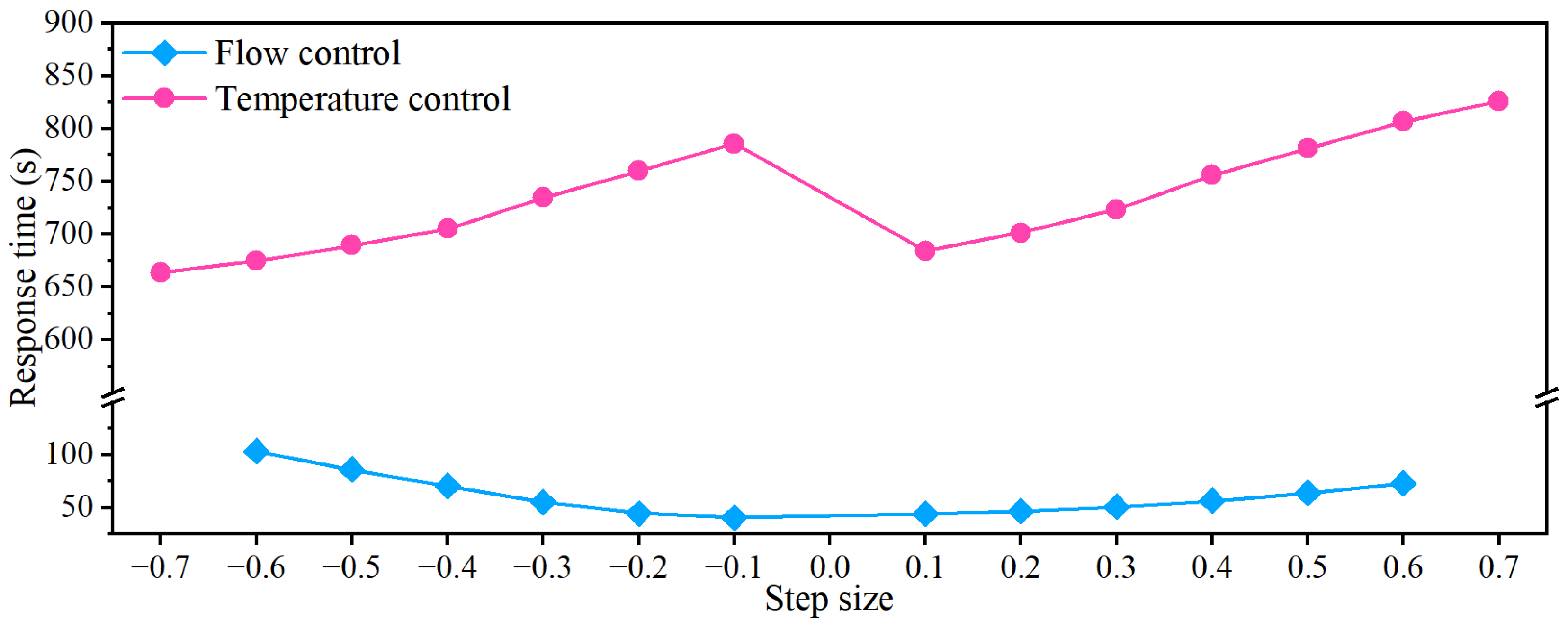
A positive step corresponds to increasing primary side flow to raise cooling capacity, while a negative step corresponds to reducing primary side flow to cut cooling output. Figure 8 shows that under the variable flow pump strategy, when the absolute step magnitude is the same, the relationship between response time and step size is essentially the same for both positive and negative steps. Larger steps take longer to reach the new steady state. This indicates that the strategy is largely insensitive to step direction and is driven mainly by step magnitude. By contrast, the cooling tower outlet temperature strategy shows stronger linearity and greater dependence on the operating point, and the positive and negative steps display opposite trends. For positive steps, small steps respond fastest, and response time lengthens as the step magnitude increases. For negative steps, small steps are slowest, and response time shortens as the absolute step magnitude grows. A plausible explanation is that larger negative steps reduce the cooling tower’s heat rejection capacity more substantially, producing larger changes in system temperature and cooling capacity. That makes it easier for the response to cross, and then approach, the new steady state threshold more quickly. The case of a step of −0.1 is particularly illustrative. It corresponds to a 5 Hz reduction from 50 Hz, which produces only a small disturbance in water temperature and cooling output. Moreover, at higher fan power operating points, the marginal temperature control effect of a given frequency change is weaker. Combined with pipework thermal inertia, this makes that operating point the slowest representative case among the negative step tests. Overall, the differences in response time between positive and negative steps are small across strategies. Even where the cooling tower outlet temperature strategy shows some directionality, the positive–negative response time gap stays within 100 s. Against its stabilization time scale of roughly 800 s, that difference is negligible and acceptable in engineering practice.

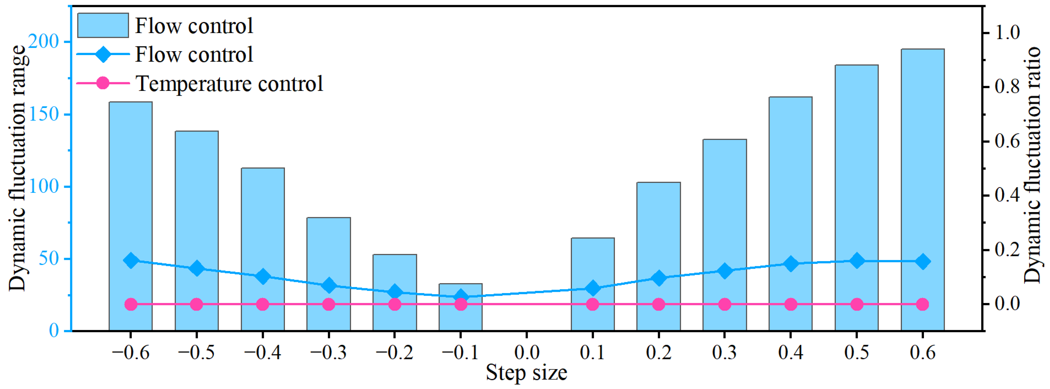
Figure 9 reports the dynamic fluctuation amplitude and the dynamic fluctuation ratio under different step magnitudes. In the figure, the bar chart and the blue square line correspond to the variable flow pump strategy, while the red circle line corresponds to the cooling tower outlet temperature strategy. The variable flow pump results follow the same pattern for positive and negative steps. Under negative steps, ΔQ_ext increases with the absolute step magnitude, rising from 33.0 kW at a step of −0.1 to 158.5 kW at −0.6, while η_Q increases from 0.027 to 0.162. Under positive steps, ΔQ_ext likewise increases as the step grows, rising from 64.3 kW at 0.1 to 195.0 kW at 0.6, and η_Q increases from 0.060 to 0.158. By contrast, the cooling tower outlet temperature strategy shows fluctuations that are effectively negligible under both directions. When the step magnitude lies between 0.2 and 0.6, both ΔQ_ext and η_Q are approximately zero, which is why Figure 9 does not display ΔQ_ext values for that strategy. Taken together, these trends indicate that under variable flow pumping, larger steps produce stronger energy disturbances and more pronounced transient swings, with both ΔQ_ext and η_Q rising monotonically with the absolute step magnitude. Under cooling tower outlet temperature control, however, both metrics remain close to zero for positive and negative steps, indicating that the strategy can effectively suppress transient fluctuations during step disturbances in either direction.

3.4. Dynamic Performance of the Combined Control Strategy

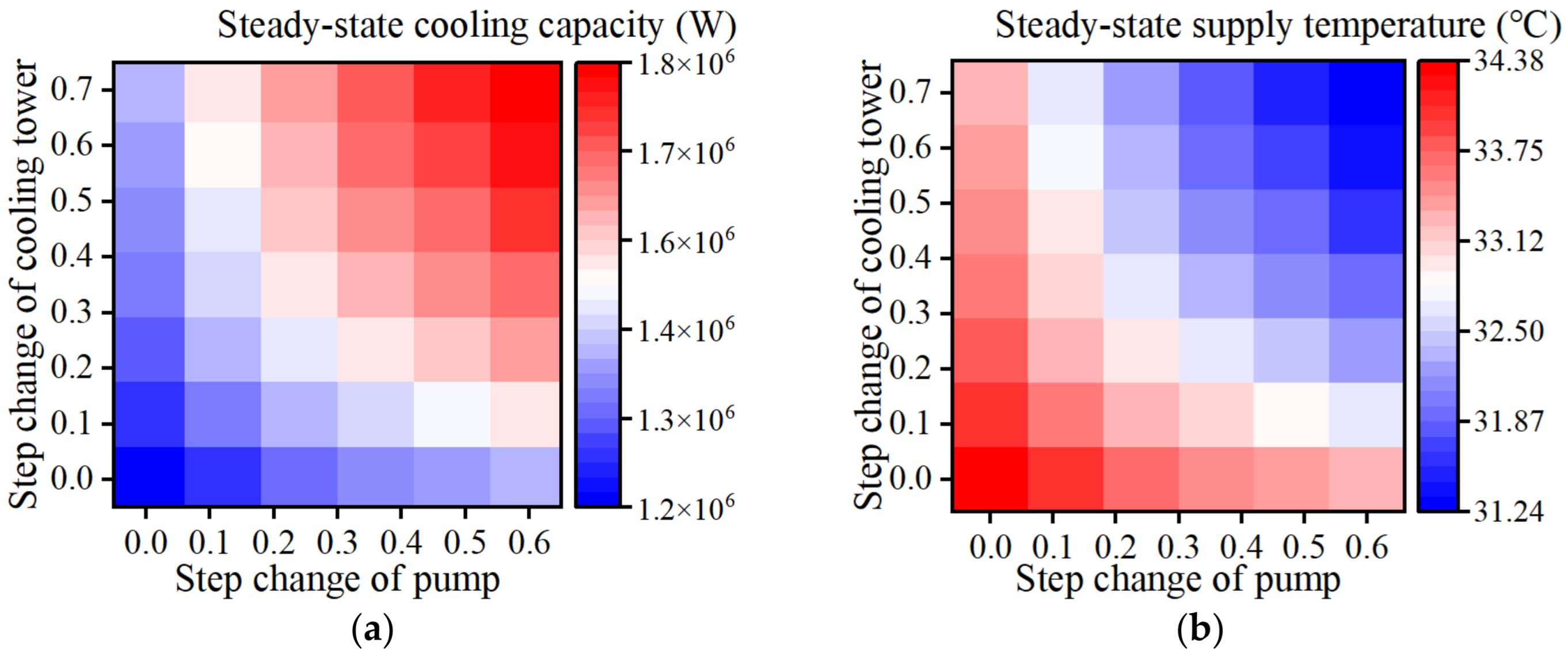
In designing the combined operating conditions, the paper treats primary side variable flow pumping and variable frequency control of the cooling tower fan as a joint regulation strategy. Figure 10 presents heat maps of the resulting steady state cooling capacity and supply water temperature. Two features are immediately apparent. First, a given target cooling output or supply temperature can be achieved by more than one combination of operating points. Second, the cooling tower side delivers a larger incremental benefit when the pump step magnitude is high. This suggests that once primary side flow is sufficiently large, heat transfer is no longer primarily constrained by the flow side. Instead, changes in cooling plant temperature contribute more decisively to steady state cooling output. Consistent with the changes in cooling capacity, steady state supply temperature falls monotonically as the two manipulated variables increase, and it also shows diminishing marginal returns. For example, with the pump step fixed at 0.6, increasing the cooling tower step from 0.1 to 0.7 reduces supply temperature from 33.27 °C to 31.25 °C. Taken together, the two panels indicate that under the combined strategy, the steady state output space is both monotonic and readily mappable. Steady state cooling capacity can be covered from about 1.18 MW up to 1.83 MW, while supply temperature can be lowered from roughly 34.37 °C to 31.25 °C.

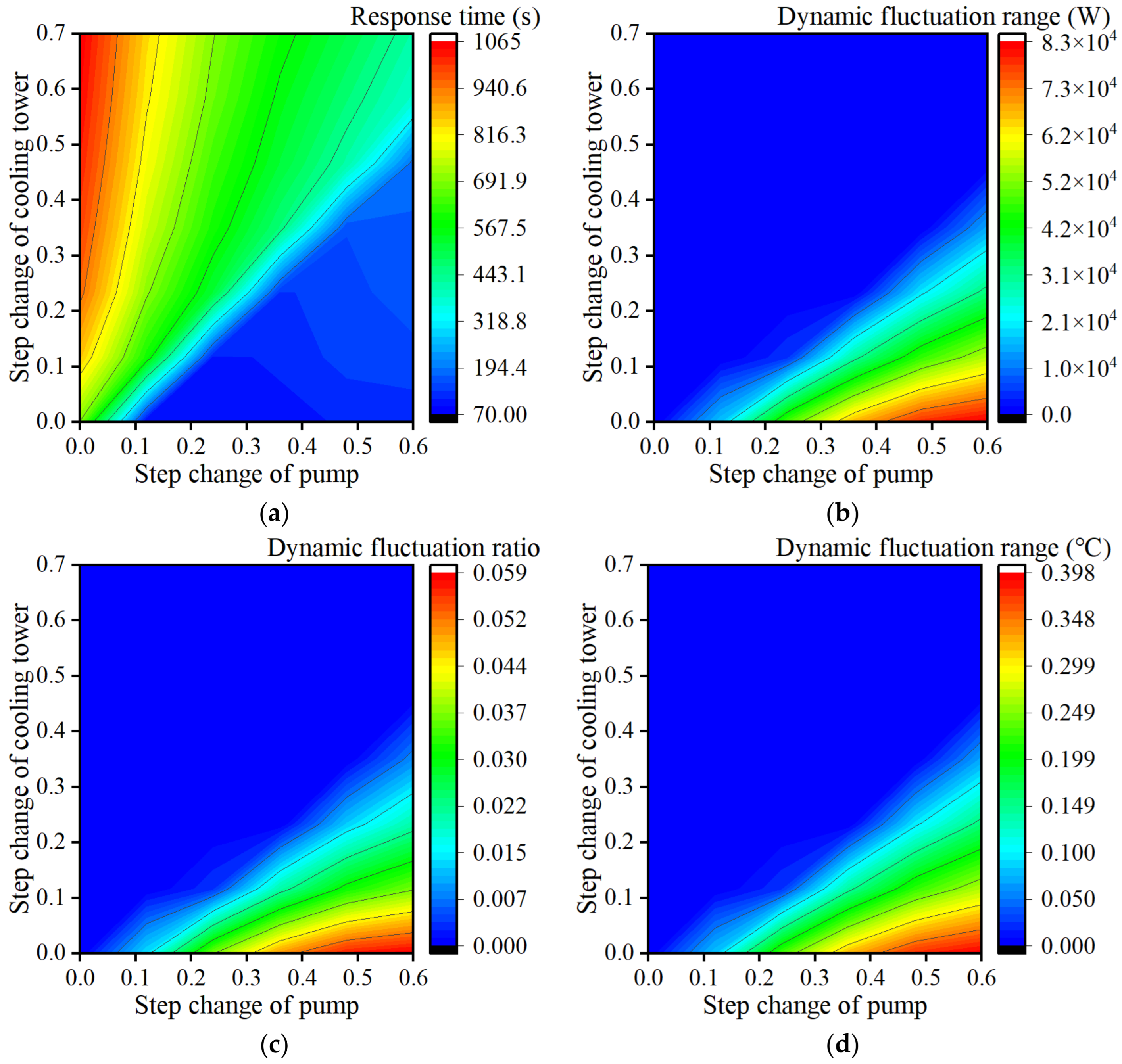
Building on the steady state cooling capacity map, the paper then embeds dynamic performance metrics into the combined condition database, producing the results shown in Figure 11. Figure 11a reveals a clear pattern in stabilization speed. In the region where the cooling tower fan step is small, system dynamics are dominated by the pump’s ability to change primary side mass flow rapidly, and response time can be compressed sharply. For instance, when the cooling tower step is 0.1, increasing the pump step from 0.1 to 0.2 reduces response time from 688.3 s to 73.7 s. Across pump steps from 0.2 to 0.6, response time remains at a comparatively low level, roughly 74.0 to 120.0 s. This suggests that when the disturbance on the cooling plant side is weak, heat transfer through the plate heat exchanger can be established quickly via flow adjustment and the system can settle rapidly.

The picture changes as the cooling tower fan step increases. Response time lengthens substantially overall, and sensitivity to the pump step diminishes. When the pump step is 0.1, raising the cooling tower step from 0.1 to 0.7 increases response time from 688.3 s to 1063.6 s. Even if the pump step is raised to 0.6, a cooling tower step of 0.6 or 0.7 still requires 375.7 s and 418.3 s, respectively, to stabilize. This indicates that in this regime the transient is governed more by cooling tower heat rejection and the thermal capacitance of the pipe network. The response time map also suggests a threshold near a cooling tower step of about 0.5, where the dominant mechanism switches between fast pump driven regulation and thermal inertia dominated behavior. For example, with a pump step of 0.5, increasing the cooling tower step from 0.3 to 0.5 raises response time from 144.5 s to 154.2 s and then triggers a sharp jump to 416.6 s.

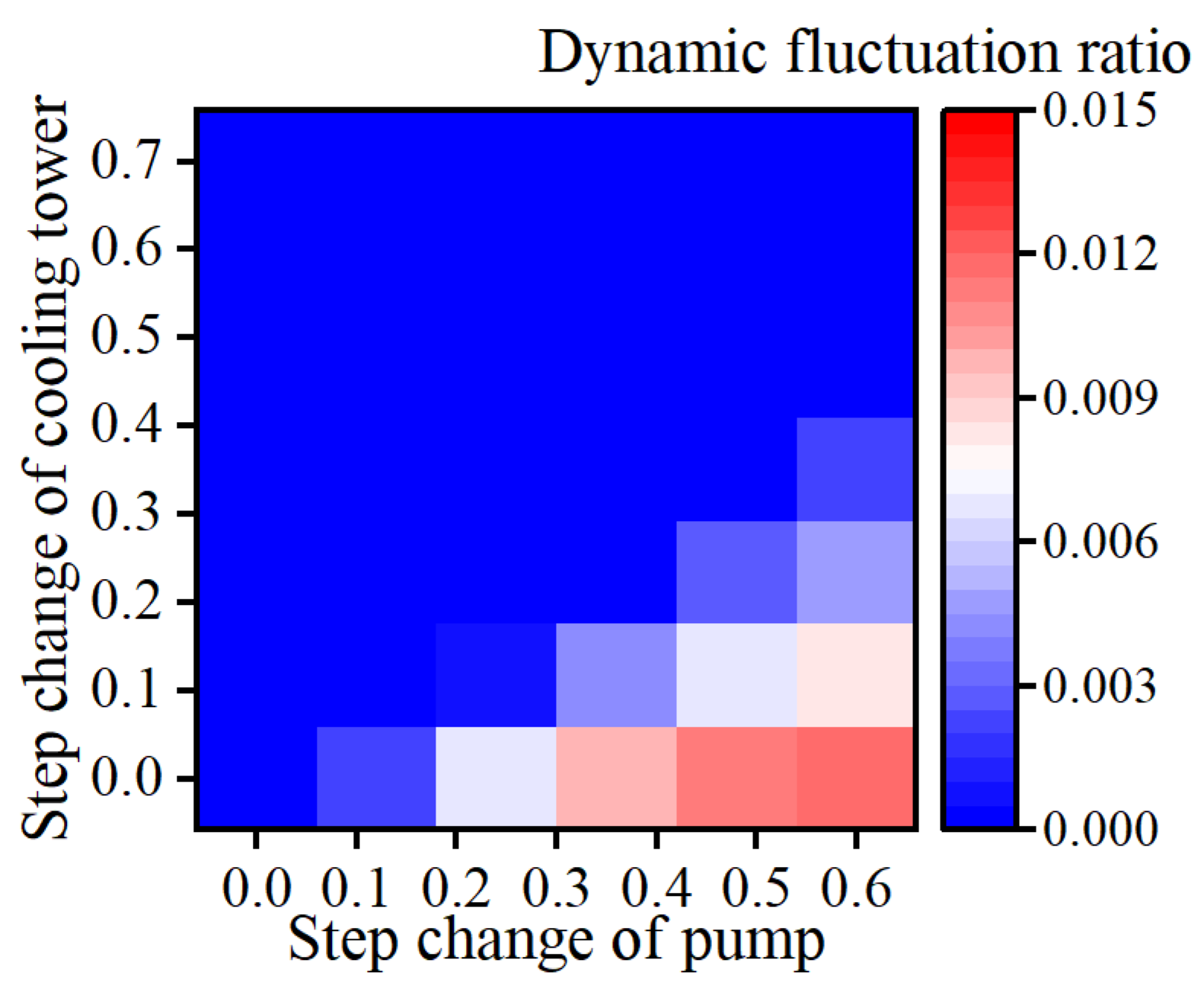
The spatial distribution of response speed aligns with where fluctuation risk concentrates. Figure 11b,c show that the dynamic fluctuation amplitude of cooling capacity grows markedly at operating points with a small cooling tower fan step and a large pump step. When the cooling tower step is 0.1, pump steps of 0.3, 0.4, 0.5, and 0.6 correspond to amplitudes of 48,298.6 W, 67,762.3 W, 79,153.3 W, and 82,961.9 W, respectively. The dynamic fluctuation ratio rises in parallel, reaching 0.05895 at a pump step of 0.6. That implies a relative deviation risk of nearly 5.9% in this region. Once the cooling tower step reaches 0.3 or higher, the fluctuation ratio falls quickly to the 10⁻² range and even down to 10⁻⁵. Many operating points show near zero fluctuation, indicating that once the cooling plant side participates in regulation, it not only increases steady state cooling capacity but also sharply suppresses transient departures in cooling output.

Figure 11d shows that the distribution of temperature fluctuation amplitude mirrors that of cooling capacity volatility. The peak again appears where the cooling tower step is small and the pump step is large. With a cooling tower step of 0.1 and a pump step of 0.6, the temperature fluctuation amplitude reaches 0.40 °C. When the cooling tower step increases to 0.2, 0.3 and 0.4, the amplitude under a pump step of 0.6 falls to 0.27 °C, 0.16 °C, and 0.07 °C, respectively. At most operating points with a cooling tower step above 0.5, the amplitude is on the order of 10⁻⁴ °C. In practical terms, the temperature response can be treated as essentially monotonic, with very low fluctuation risk.

3.5. Engineering Validation of the Optimisation Results

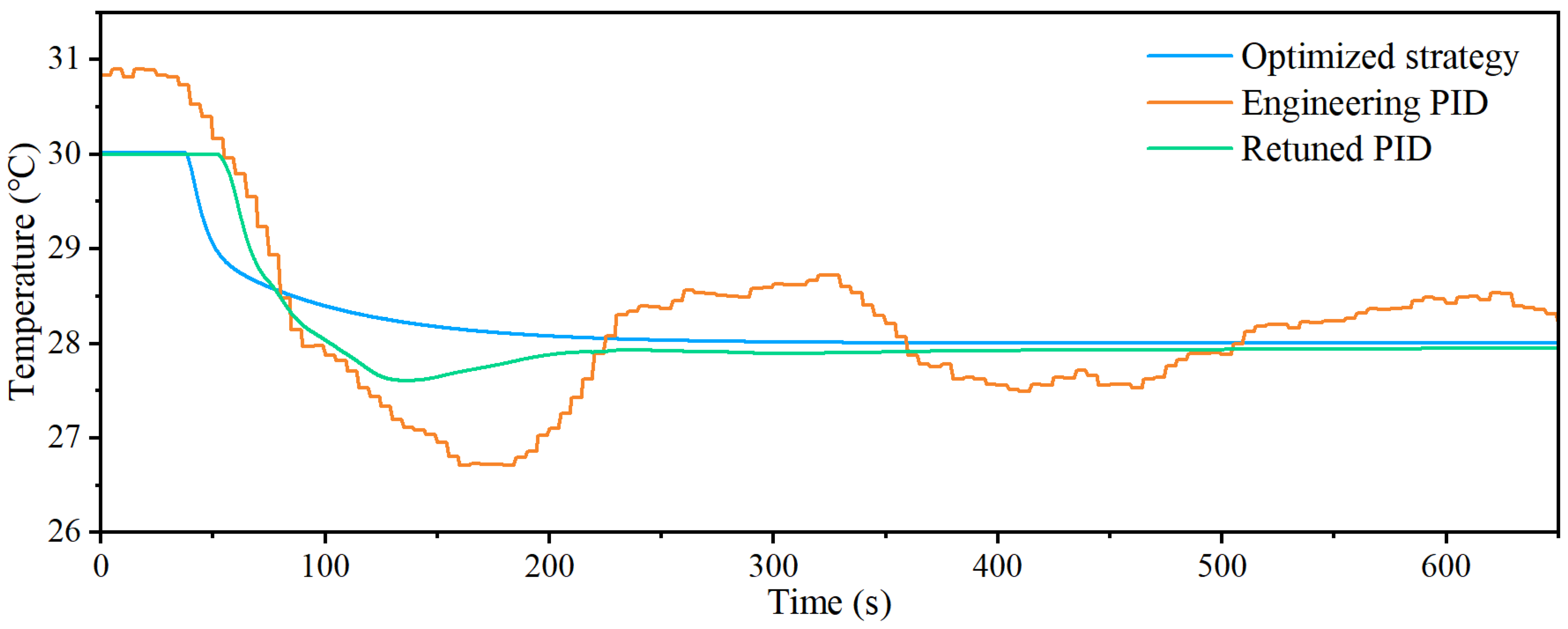
Our optimized strategy is implemented as an explicit mapping policy computed offline and executed online via table lookup, which is straightforward to integrate into existing BAS logic. Offline, we use the calibrated Modelica model to batch-simulate the combined operating condition database and screen candidate operating points with the transient-risk metrics, thereby generating a mapping from the target cooling demand (ΔQ_target) or an equivalent target supply temperature change (ΔT_target) to the optimal actuator pair. Online, the BAS estimates ΔQ_target or ΔT_target from the measured IT load change and or the supply temperature deviation after a setpoint update and queries a two-dimensional lookup table using either nearest neighbor selection or bilinear interpolation. In addition, to address the concern that the measured onsite PID baseline may not represent best-practice tuning, we additionally implemented a retuned PID baseline using the same setpoint-change event and the same measurement stream; it is reported alongside the as-is engineering PID in Figure 12, while the retuning procedure and best-practice rationale are provided in Appendix C. Under a setpoint change from 30 °C to 28 °C as shown in Figure 13, the field engineering PID exhibits a transient response dominated by latency and inertia. The temperature drops below the target to 26.71 °C, corresponding to ΔT_ext of approximately 1.29 °C, then rebounds to about 28.72 °C and continues to oscillate, indicating a prolonged settling process and elevated transient temperature risk. Retuning reduces the undershoot to 27.61 °C, with ΔT_ext of approximately 0.39 °C, and largely suppresses the rebound. However, the settling time remains relatively long under the prevailing latency. In contrast, the optimized strategy yields an almost monotonic transition, reaches and maintains approximately 28 °C, and limits the undershoot to less than 0.01 °C. These results suggest that the improvement is not attributable solely to PID gain adjustment but instead arises primarily from latency aware operating point selection enabled by the explicit policy database.

In terms of dynamic response time, the optimized strategy curve converges smoothly and monotonically after the setpoint change. The engineering PID exhibits steady-state drift, with the supply temperature settling at 28.42 °C, and it also shows a pronounced undershoot: the minimum temperature drops to about 26.7 °C. Its ΔT_ext is 1.71 °C and η_T is 6.01%. By contrast, the retuned PID achieves a steady-state temperature of 27.95 °C, closer to the target; its ΔT_ext is 0.341 °C and η_T is 1.22 × 10⁻², but the settling time remains relatively long at 533 s. This pattern reflects a familiar limitation of conventional PID control in practice: it often adjusts to a new setpoint without explicitly constraining system inertia and control chain delays. Most notably, the optimized strategy model predictive control curve regulates smoothly, with ΔT_ext is 3.10 × 10⁻⁵ °C and η_T is 1.11 × 10⁻⁶, and it maintains a shorter settling time of 415.9 s. The fluctuation metrics are essentially zero, and there is no secondary swing of the “undershoot then rebound” type. In short, the proposed strategy unifies steady state target matching with explicit control of transient cost. In engineering comparison, that translates into a shorter stabilization time and a materially lower fluctuation risk.

4. Discussion

4.1. Control-Pathway Interpretation of the Investigated Strategies

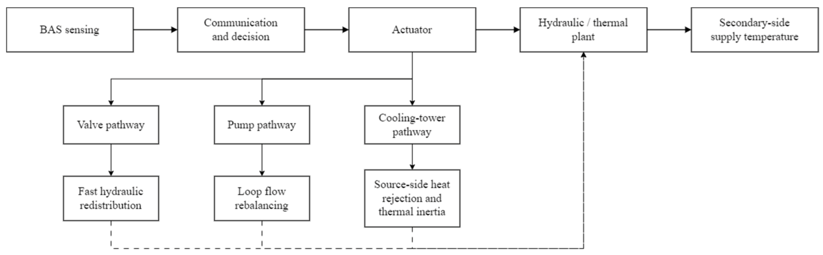
The three single-actuator strategies show markedly different dynamic behaviors because they act through different control pathways. In the present liquid-cooling system, the control command propagates from BAS sensing and supervisory decision making to actuator motion, hydraulic and thermal process evolution, CDU heat exchange, and finally the secondary-side supply temperature. Accordingly, the valve, pump, and cooling-tower fan do not affect the controlled output through the same pathway, and, therefore, differ in effective delay, dominant time constant, and pathway bandwidth. The control-pathway differences among the three strategies are summarized schematically in Figure 13.

Valve control acts primarily through a fast hydraulic redistribution pathway. Once the delay is overcome, the heat-transfer condition across the CDU changes rapidly, which explains the shortest response among the three strategies. However, because the hydraulic state changes faster than the source-side thermal balance can re-establish, valve control is also more prone to transient deviation and fluctuation risk.

Pump control also acts through the primary-side flow pathway, but in a more distributed manner across the circulation loop. Its delay is similar to that of valve control, while its dominant time constant is larger. As a result, pump control remains fast but produces a smoother response, representing a more balanced trade-off between tracking speed and transient stability.

Cooling-tower fan control acts through the source-side heat-rejection pathway rather than through direct flow redistribution. Its effect must propagate through the cooling tower, the primary loop, and the CDU before it appears in the secondary-side supply temperature. This makes it a thermal-inertia-dominated pathway with the largest time constant and the lowest effective bandwidth. Consequently, it produces an almost monotonic response with negligible overshoot, but it is much slower than the flow-based strategies.

As shown by the quantitative results in Table 3 of Section 3.2.5 and the related analysis, the observed differences can be interpreted as pathway-dependent differences in delay and bandwidth. From a frequency-domain perspective, the effective bandwidth ranking is valve > pump ≫ cooling tower, which is fully consistent with the time-domain results.

4.2. Comparison of the Present Findings with Existing Literature

Most existing studies on liquid-cooled data center optimization focus on steady-state energy efficiency, operating-point selection, or annual performance under varying ambient conditions [18,19,20,21,22]. These studies are highly valuable for energy-efficient operation, but they pay less attention to the transient cost and risk introduced by control-chain latency and thermal inertia during load changes. In contrast, the present study addresses delay-aware transient-safe operation, with emphasis on response speed, fluctuation risk, and engineering applicability.

Compared with prior dynamic thermal-response studies in HVAC and radiant systems [26,27,28,29], this work adapts process-oriented dynamic evaluation to the liquid-cooled data center context. The proposed framework combines dynamic response time, fluctuation amplitude, and fluctuation ratio under a standardized step-test protocol, thereby making transient performance comparable across different control strategies. The stricter 99.6% settling criterion further reflects the tighter stability requirements of high-value liquid-cooled computing platforms.

The present study is also distinct from representative advanced control approaches. The present study is also distinct from representative advanced control approaches. Recent studies have reported robust data-driven MPC and collaborative MPC strategies with stronger capability in handling constraints, multivariable coordination, and uncertainty [39,40]. However, such methods usually require higher online computational capability, more elaborate predictive models, and a more sophisticated implementation environment. By contrast, the present method is not designed as a new online advanced controller. Its contribution lies in combining an offline calibrated dynamic model, transient-risk screening, and online explicit operating-point lookup to form a low-complexity and BAS-deployable coordination strategy. A comparison between the present strategy and representative advanced control approaches is provided in

Table 4. Comparison between the proposed strategy and representative control methods.

Method	Representative Literature	Core Characteristic	Model Requirement	Online Optimization	Constraint Handling	Online Computational Burden	Position Relative to this Study
Classical PID/PI control	Grimholt and Skogestad [25]	Low-order feedback control based on measured error	Low	No	Weak	Very low	Engineering baseline without explicit delay-aware operating-point selection
Robust data-driven MPC	Li et al. [40]	Predictive control with data-driven thermal model and uncertainty handling	Medium	Yes	Strong	Medium to high	More powerful online optimization, but higher deployment complexity
Collaborative MPC	Zhao et al. [39]	Component-level coordinated predictive optimization	High	Yes	Strong	High	Suitable for richer sensing and computation in tightly coupled systems
This study	Present work	Offline dynamic database plus online explicit operating-point lookup	Medium (offline calibrated model)	No	Moderate through offline screening	Very low	Low-complexity BAS-deployable delay-aware explicit coordination strategy

.

Therefore, the advantage of this study relative to the existing literature is not the proposal of a more sophisticated online optimizer, but the establishment of a delay-aware and engineering-interpretable coordinated-control framework that links dynamic modeling, transient-risk evaluation, and practical operating-point selection.

4.3. Environmental Boundary Effects and Applicability

Outdoor environmental parameters affect the system by changing the source-side thermal boundary. In the cooling-tower-direct liquid-cooling system studied here, ambient wet-bulb temperature is a key boundary condition because it directly affects cooling-tower heat rejection and, in turn, the primary-side temperature level and the CDU heat-transfer capacity.

The cooling-tower representation adopts the YorkCalc correlation without explicitly modeling tower-internal solid thermal masses (e.g., fill and basin) as separate thermal nodes, which may underestimate additional tower-internal delay under very large disturbances. Nonetheless, the minute-scale inertia observed under source-side temperature manipulation is primarily governed by loop water thermal capacitance and transport delay, which are explicitly captured via first-order delay/mixed-volume formulations. Consequently, the qualitative conclusion—source-side temperature manipulation being inertia-dominated—is expected to remain consistent, and is likely transferable to alternative cooling sources (e.g., chillers or air-cooled units) given comparable loop inventory and transport delay.

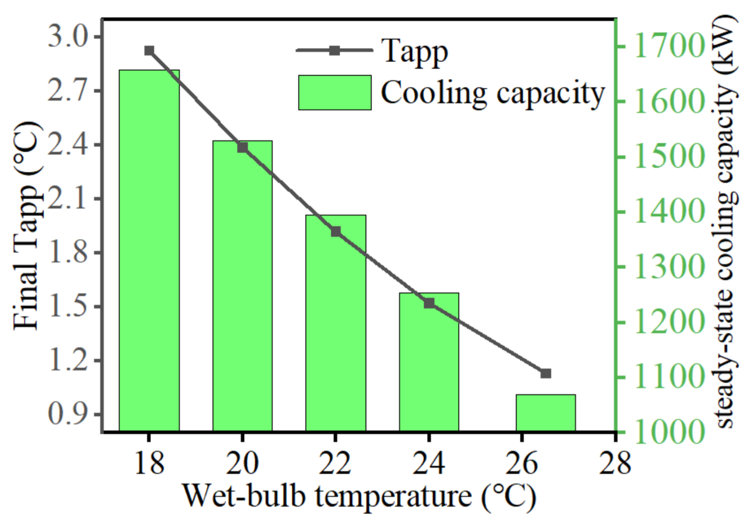
As shown in Appendix D, increasing wet-bulb temperature systematically changes the final Tapp and reduces the achievable steady-state cooling capacity of the system. By contrast, the response time of the variable water-temperature strategy increases only slightly, while the dynamic fluctuation ratio remains close to zero across the tested cases. This indicates that environmental variation mainly shifts the steady-state thermal boundary and cooling-capacity level, rather than fundamentally changing the dynamic response pattern of the cooling-tower variable water-temperature strategy. The environmental boundary effects under different wet-bulb conditions are summarized in Figure 14.

The present conclusions are obtained for a specific liquid-cooling platform and a calibrated dynamic model, so the numerical optimum remains configuration-dependent. Nevertheless, the broader interpretation remains transferable: environmental parameters primarily act as boundary conditions on source-side thermal performance, and their influence should be incorporated explicitly when coordinated control strategies are designed for different climates and operating envelopes.

On this basis, future work can be extended toward combined-condition sensitivity analysis under varying outdoor environmental parameters. Wet-bulb temperature, dry-bulb temperature, and load disturbance can be treated jointly as external boundary conditions for system operation, and environment-aware coordinated pump–fan optimization can then be developed to improve dynamic robustness and control coordination under different climates and load fluctuations.

4.4. Hierarchical Summary of Contributions

The contributions of this study can be summarized hierarchically as follows.

• Delay-aware system-level modeling contribution: This study develops and validates a delay-aware dynamic Modelica model for a liquid-cooled data center cooling system. Unlike studies that treat the cooling plant mainly from a steady-state or quasi-steady perspective, the present model explicitly incorporates control-chain delay, transport delay, and thermal inertia within a unified plant-level framework. This provides the basis for reproducing and interpreting actuator-dependent transient behavior under abrupt load-responsive operation.
• Transient-performance evaluation contribution: This study proposes a standardized percentage step-test framework together with three transient metrics, namely dynamic response time, dynamic fluctuation amplitude, and dynamic fluctuation ratio. By combining these indicators under a unified settling criterion, the work converts transient cost and fluctuation risk into directly comparable quantities across different control strategies. The use of the 99.6% settling threshold further strengthens the engineering relevance of the framework for high-value liquid-cooled computing scenarios requiring tighter thermal stability.
• Control-pathway and mechanism interpretation contribution: Beyond reporting engineering phenomena, this study provides a control-oriented interpretation of the actuator-dependent differences among valve control, pump control, and cooling-tower fan control. The identified differences in effective delay, dominant time constant, and effective bandwidth clarify why valve control is fastest but more fluctuation-prone, pump control offers a more balanced trade-off, and cooling-tower control is slow but highly stable. In this sense, the study elevates the comparison of single-actuator strategies from empirical observation to a physically interpretable control-pathway analysis.
• Coordinated control and deployable strategy contribution: Building on the above modeling and evaluation framework, this study further develops a coordinated pump–fan operating strategy through operating-point matching and transient-risk screening. The key innovation is not the proposal of a new online advanced controller, but the establishment of a low-complexity, delay-aware, and BAS-deployable explicit coordination framework that reallocates control authority between fast flow-side actuation and slow source-side thermal regulation. This provides a practical path for achieving both faster convergence and lower fluctuation risk in engineering operation.

Taken together, the novelty of this work lies not in a single isolated result, but in a hierarchical framework consisting of delay-aware modeling, transient-risk evaluation, mechanism-level control interpretation, and deployable coordinated control design.

4.5. Limitations and Future Work

Several limitations remain, and future work can be extended in the following directions:

• The current validation range remains limited: Model validation and strategy comparison are mainly conducted under a limited set of standardized step disturbances. Therefore, absolute metrics such as response time and fluctuation amplitude remain dependent on the specific system configuration, operating point, and environmental boundary conditions. Further validation is needed under wider climate conditions and more complex load trajectories.
• Multi-loop coupling has not been fully resolved: The present study mainly focuses on plant-side delay-sensitive dynamics, while the fast local secondary-side regulation is treated as a boundary condition. In real liquid-cooling systems, more complex dynamic coupling may exist between the primary- and secondary-side control loops. Future work should therefore consider explicit dual-loop modeling and coordinated optimization.
• Environmental-boundary analysis is still limited to single-parameter variation: The current discussion and appendix-based analysis mainly focus on wet-bulb temperature. The main conclusion is that environmental variation primarily shifts the steady-state thermal boundary and the final cooling-capacity level, while having limited influence on the dynamic characteristics of the variable water-temperature strategy. Future work should extend this analysis by treating wet-bulb temperature, dry-bulb temperature, and load disturbance as combined boundary conditions.
• The current optimization does not explicitly include energy as an objective: At the present stage, the optimization mainly prioritizes response speed under a fluctuation constraint, and, therefore, emphasizes the trade-off between speed and stability. The additional energy cost during transient regulation is not yet included as an explicit objective. Future work may introduce event-level energy metrics and establish a multi-objective framework that jointly considers response speed, fluctuation risk, and energy penalty.
• The control framework can be extended to a higher level: The proposed method is essentially a low-complexity coordinated strategy based on an offline database and online explicit lookup, which gives it strong engineering deployability. In future work, this advantage can be retained while integrating surrogate models, boundary-aware coordinated optimization, or time-varying delay modeling to further improve the robustness and adaptability of the pump–fan coordinated strategy under complex environmental boundaries.

5. Conclusions

The main conclusions of this study can be summarized as follows:

• Delay-aware system-level modeling contribution: A delay-aware Modelica model was developed and validated for a liquid-cooled data-center cooling system. Under the engineering setpoint-change event from 30 °C to 28 °C, the model reproduced the dominant temporal trends and turning-point behavior of the measured plant response. After excluding the start-up transient and evaluating the interval from 100 s to 655 s, the maximum error of the secondary-side supply temperature decreased from 1.71 °C to 0.68 °C, while the RMSE decreased from 0.48 °C to 0.26 °C. These results indicate that the model is suitable for plant-level dynamic analysis of secondary-side supply temperature under abrupt operating changes.
• Transient-performance evaluation contribution: A standardized percentage step-test framework was established together with three transient metrics, namely dynamic response time, dynamic fluctuation amplitude, and dynamic fluctuation ratio. Using a 99.6% settling criterion, this framework enabled direct comparison of different control strategies under the same disturbance definition. The results show that the framework can clearly quantify the trade-off between response speed and fluctuation risk. For example, under single-actuator positive steps, the response time remained at 38.3–41.3 s for valve control, increased from 44.2 s to 72.9 s for variable-flow pump control, and rose to 684.3–825.9 s for cooling-tower outlet temperature control, while the corresponding fluctuation behaviors differed markedly across strategies.
• Control-strategy and coordinated-control contribution: Among the three single-actuator strategies, constant differential pressure valve control was the fastest but also the most fluctuation-prone. As the valve step increased from 0.1 to 0.7, the cooling-capacity overshoot increased from 91.6 kW to 476.9 kW, and the dynamic fluctuation ratio increased from 9.2% to 38.7%. Variable-flow pump control provided a more balanced trade-off between speed and smoothness: its response time ranged from 44.2 s to 72.9 s, and the maximum cooling-capacity overshoot at the largest step was 195 kW with a fluctuation ratio of about 15.8%. Cooling-tower outlet temperature control was the most stable but much slower, with response times of 684.3–825.9 s and a maximum overshoot of only 6.6 kW. Building on these pathway differences, the proposed coordinated pump–fan strategy reallocated control authority across operating conditions and reduced the response time from 688.3 s to 73.7 s under fluctuation constraints, while lowering the dynamic temperature-deviation risk by up to 1.3 °C in the engineering comparison.

References

1. Ma, Y.Z.; Ma, G.Y.; Zhang, S.; Xu, S.X. Experimental investigation on a novel integrated system of vapor compression and pump driven two phase loop for energy saving in data centers cooling. Energy Convers. Manag. 2015, 106, 194–200. [Google Scholar] [CrossRef]
2. Wang, X.Y.; Li, H.; Wang, Y.Z.; Zhao, J.; Zhu, J.B.; Zhong, S.Y.; Li, Y. Energy, exergy, and economic analysis of a data center energy system driven by CO2 ground source heat pump: Prosumer perspective. Energy Convers. Manag. 2021, 232, 113877. [Google Scholar] [CrossRef]
3. Qian, X.D.; Li, Z.; Li, Z.X. A thermal environmental analysis method for data centers. Int. J. Heat Mass Transf. 2013, 62, 579–585. [Google Scholar] [CrossRef]
4. Nada, S.A.; El Zoheiry, R.M.; Elsharnoby, M.; Osman, O.S. Experimental investigation of hydrothermal characteristics of data center servers’ liquid cooling system for different flow configurations and geometric conditions. Case Stud. Therm. Eng. 2021, 27, 101276. [Google Scholar] [CrossRef]
5. Zhang, Y.B.; Shan, K.; Li, X.M.; Li, H.X.; Wang, S.W. Research and Technologies for next generation high temperature data centers State of the arts and future perspectives. Renew. Sustain. Energy Rev. 2023, 171, 112991. [Google Scholar] [CrossRef]
6. Zhou, F.; Gu, W.; Ma, G. Advancements in data center cooling systems: From refrigeration to high performance cooling. Energy Build. 2024, 320, 114634. [Google Scholar] [CrossRef]
7. Zhang, Y.; Zhang, Y.; Bakir, M.S. Thermal Design and Constraints for Heterogeneous Integrated Chip Stacks and Isolation Technology Using Air Gap and Thermal Bridge. IEEE Trans. Compon. Packag. Manuf. Technol. 2014, 4, 1914–1924. [Google Scholar] [CrossRef]
8. Qu, S.; Duan, K.; Guo, Y.; Pan, L.; Zhang, H.; Wang, S. Real time optimization of the liquid cooled data center based on cold plates under different ambient temperatures and thermal loads. Appl. Energy 2024, 363, 123101. [Google Scholar] [CrossRef]
9. Azarifar, M.; Arik, M.; Chang, J.Y. Liquid cooling of data centers: A necessity facing challenges. Appl. Therm. Eng. 2024, 247, 123112. [Google Scholar] [CrossRef]
10. Wu, X.L.; Yang, J.L.; Liu, Y.; Yang, Z.; Li, H.; Zhang, J.F. Investigations on heat dissipation performance and overall characteristics of two phase liquid immersion cooling systems for data center. Int. J. Heat Mass Transf. 2025, 239, 126575. [Google Scholar] [CrossRef]
11. Ge, J.L.; Xia, F.F.; Zhang, C.B.; Zhai, X.W.; Guo, W. Performance Enhancement of Single Phase Immersion Liquid Cooled Data Center Servers. J. Therm. Sci. 2024, 33, 1757–1772. [Google Scholar] [CrossRef]
12. Huang, Y.P.; Liu, C.D.; Zhong, Y.F.; Han, X.; Feng, X.F. Experimental study on jet enhanced immersion liquid cooling for energy efficient data centers. Energy 2025, 334, 137584. [Google Scholar] [CrossRef]
13. He, W.; Zhang, J.F.; Li, H.L.; Ding, S.; Yang, B.; Huang, S.; Yan, J. Effects of different water cooled heat sinks on the cooling system performance in a data center. Energy Build. 2023, 292, 113162. [Google Scholar] [CrossRef]
14. Li, J.; Luo, X.; Wang, M.; Ma, G. Study of flow and heat transfer characteristics of tandem cold plates for data center cooling. Case Stud. Therm. Eng. 2025, 73, 106590. [Google Scholar] [CrossRef]
15. Heydari, A.; Shahi, P.; Radmard, V.; Eslami, B.; Chowdhury, U.; Saini, S.; Bansode, P.; Miyamura, H.; Agonafer, D.; Rodriguez, J. Liquid to liquid cooling for high heat density liquid cooled data centers. In Proceedings of the ASME International Technical Conference and Exhibition on Packaging and Integration of Electronic and Photonic Microsystems (InterPACK), Garden Grove, CA, USA, 25–27 October 2022; p. V001T01A007. [Google Scholar]
16. Chang, Q.K.; Huang, Y.F.; Liu, K.Y.; Xu, X.; Zhao, Y.H.; Pan, S. Optimization Control Strategies and Evaluation Metrics of Cooling Systems in Data Centers: A Review. Sustainability 2024, 16, 7222. [Google Scholar] [CrossRef]
17. Shao, X.T.; Zhang, Z.B.; Song, P.; Feng, Y.Z.; Wang, X.L. A review of energy efficiency evaluation metrics for data centers. Energy Build. 2022, 271, 112308. [Google Scholar] [CrossRef]
18. He, W.; Ding, S.; Zhang, J.F.; Li, H.L.; Yang, B.; Yan, J.; Huang, S. Performance optimization of server water cooling system based on minimum energy consumption analysis. Appl. Energy 2021, 303, 117620. [Google Scholar] [CrossRef]
19. He, W.; Zhang, J.F.; Li, H.L.; Ding, S.; Yang, B.; Huang, S.; Yan, J. Optimal thermal management of server cooling system based cooling tower under different ambient temperatures. Appl. Therm. Eng. 2022, 207, 118176. [Google Scholar] [CrossRef]
20. Wang, S.Q.; Tu, R.; Chen, X.Z.; Duan, Y.Y.; Xia, X.Y. Thermal performance analyses and optimization of data center centralized cooling system. Appl. Therm. Eng. 2023, 222, 119817. [Google Scholar] [CrossRef]
21. Li, J.J.; Li, Z.W. Model based optimization of free cooling switchover temperature and cooling tower approach temperature for data center cooling system with water side economizer. Energy Build. 2020, 227, 110407. [Google Scholar] [CrossRef]
22. Song, W.S.; Hong, S.H.; Park, T.J. The effects of service delays on a BACnet based HVAC control system. Control Eng. Pract. 2007, 15, 209–217. [Google Scholar] [CrossRef]
23. Price, C.; Park, D.; Rasmussen, B.P. Cascaded Control for Building HVAC Systems in Practice. Buildings 2022, 12, 1814. [Google Scholar] [CrossRef]
24. Grimholt, C.; Skogestad, S. Optimal PID Control on First Order Plus Time Delay Systems & Verification of the SIMC Rules. IFAC Proc. Vol. 2013, 46, 265–270. [Google Scholar] [CrossRef]
25. Ning, B.; Schiavon, S.; Bauman, F.S. A novel classification scheme for design and control of radiant system based on thermal response time. Energy Build. 2017, 137, 38–45. [Google Scholar] [CrossRef]
26. Krajčík, M.; Šikula, O. Heat storage efficiency and effective thermal output: Indicators of thermal response and output of radiant heating and cooling systems. Energy Build. 2020, 229, 110524. [Google Scholar] [CrossRef]
27. Chen, Q.; Li, N. Thermal response time prediction based control strategy for radiant floor heating system based on Gaussian process regression. Energy Build. 2022, 263, 112044. [Google Scholar] [CrossRef]
28. Qi, D.; Liu, Y.; Zhao, C.; Dong, Y.; Song, B.; Li, A. Thermal response and performance evaluation of floor radiant heating system based on fuzzy logic control. Energy Build. 2024, 313, 114232. [Google Scholar] [CrossRef]
29. Wang, M.Z.; Hu, E.; Chen, L. Radiation-enhanced thermal diode tank (RTDT) for refrigeration and air-conditioning (RAC) systems. Int. J. Refrig. 2023, 146, 237–247. [Google Scholar] [CrossRef]
30. Yu, R.W.; Fan, S.H. Time-modulated near-field radiative heat transfer. Proc. Natl. Acad. Sci. USA 2024, 121, e2401514121. [Google Scholar] [CrossRef]
31. Akbarzadeh, S.; Sefidgar, Z.; Valipour, M.S.; Elmegaard, B.; Arabkoohsar, A. A comprehensive review of research and applied studies on bifunctional heat pumps supplying heating and cooling. Appl. Therm. Eng. 2024, 257, 124280. [Google Scholar] [CrossRef]
32. Wang, M.Z.; Hu, E.R.; Chen, L. TRNSYS Simulation of a Bi-Functional Solar-Thermal-Energy-Storage-Assisted Heat Pump System. Energies 2024, 17, 3376. [Google Scholar] [CrossRef]
33. Sangi, R.; Müller, D. Dynamic modelling and simulation of a slinky coil horizontal ground heat exchanger using Modelica. J. Build. Eng. 2018, 16, 159–168. [Google Scholar] [CrossRef]
34. Abugabbara, M.; Lindhe, J.; Javed, S.; Bagge, H.; Johansson, D. Modelica based simulations of decentralised substations to support decarbonisation of district heating and cooling. Energy Rep. 2021, 7, 465–472. [Google Scholar] [CrossRef]
35. Dumont, É. Mass Transfer in Multiphasic Gas/Liquid/Liquid Systems. KLa Determination Using the Effectiveness Number of Transfer Unit Method. Processes 2018, 6, 156. [Google Scholar] [CrossRef]
36. Benton, D.J.; Bowman, C.F.; Hydeman, M.; Miller, P. An improved cooling tower algorithm for the CoolTools™ simulation model. ASHRAE Trans. 2002, 108, 760–768. [Google Scholar]
37. Zhu, J. Modeling, Simulation and Control Strategy Optimization of a Centralized Cooling Station Based on Modelica. Master’s Thesis, Tianjin University, Tianjin, China, 2019. [Google Scholar]
38. Liu, C.; Yu, H. Evaluation and Optimization of a Two-Phase Liquid-Immersion Cooling System for Data Centers. Energies 2021, 14, 1395. [Google Scholar] [CrossRef]
39. Zhao, J.; Hou, J.W.; Yang, Z.L.; Liu, D.H.; Xu, B.T.; Zhang, W.L.; Yao, M.; Cui, J.J.; Liu, S.P.; Qi, X.Q.; et al. Collaborative model predictive control for indirect evaporative cooling systems in data centers based on dynamic hot-spot tracking. Energy 2026, 344, 139888. [Google Scholar] [CrossRef]
40. Li, Y.R.; Yang, C.; Xia, Y.Q. A robust data-driven model predictive thermal control for rack-based data center. J. Build. Eng. 2024, 98, 110877. [Google Scholar] [CrossRef]
41. Sermsuk, M.; Sukjai, Y.; Wiboonrat, M.; Kiatkittipong, K. Utilising Cold Energy from Liquefied Natural Gas (LNG) to Reduce the Electricity Cost of Data Centres. Energies 2021, 14, 6269. [Google Scholar] [CrossRef]
42. Vertiv™ CoolChip CDU: In-Rack Liquid-to-Liquid Coolant Distribution Unit. Available online: https://www.vertiv.com/4a1992/globalassets/shared/vertiv-coolchip-cdu-100_datasheet_en.pdf (accessed on 5 March 2026).
43. Xia, L.; Wu, J.F.; Khosravi, A.; Sun, L. Modelica based modelling and control design of counter-flow SOFC system considering temperature distribution. Energy 2025, 331, 137011. [Google Scholar] [CrossRef]
44. Sanchis, R.; Peñarrocha-Alós, I. Optimal tuning of PID controllers with derivative filter for stable processes using three points from the step response. ISA Trans. 2023, 143, 596–610. [Google Scholar] [CrossRef]
45. Lawrence Berkeley National Laboratory. Buildings.Fluid.HeatExchangers.CoolingTowers.Correlations. Available online: https://simulationresearch.lbl.gov/modelica/releases/v12.0.0/help/Buildings_Fluid_HeatExchangers_CoolingTowers_Correlations.html (accessed on 14 April 2026).
Figure 1. Schematic of the data center liquid cooling system and the internal structure of the Coolant Distribution Unit (CDU): (a) Liquid Cooling System Schematic; (b) Internal Structure of the CDU.
Buildings 16 01752 g001
Figure 2. Dynamic liquid cooling system simulation model.
Buildings 16 01752 g002
Figure 3. Time series comparison of measured and simulated temperatures: (a) Primary side valve opening (Time Series); (b) Primary side flow rate (Time Series); (c) Secondary side Supply Temperature (Time Series); (d) Primary side Return Water Temperature (Time Series).
Buildings 16 01752 g003
Figure 4. System Responses Under Constant Differential Pressure Valve Control. The legend values from 0.1 to 0.7 denote valve step changes from 10% to 70%: (a) Cooling Capacity (Time Series); (b) Secondary side Supply Temperature (Time Series).
Buildings 16 01752 g004
Figure 5. System Responses Under Variable Flow Pump Control. The legend values from 0.1 to 0.6 denote primary side pump step changes from 10% to 60%: (a) Cooling Capacity (Time Series); (b) Secondary side Supply Temperature (Time Series).
Buildings 16 01752 g005
Figure 6. System Responses Under Cooling Tower Outlet Temperature Control. The legend values from 0.1 to 0.7 denote cooling tower fan step changes from 10% to 70%: (a) Cooling Capacity (Time Series); (b) Secondary side Supply Temperature (Time Series).
Buildings 16 01752 g006
Figure 7. Dynamic Response Time Across Strategies. Both y-axes show response time. Under flow control strategies (Valve Control and Pump Control), the response time of the primary side inlet temperature is on a different order of magnitude from the other variables; therefore, a dual y-axis is used: (a) Constant Differential Pressure Valve Control; (b) Variable Flow Pump Control; (c) Cooling Tower Outlet Temperature Control; (d) Cross-Strategy Comparison.
Buildings 16 01752 g007
Figure 8. Response time under positive and negative steps.
Buildings 16 01752 g008
Figure 9. Dynamic fluctuation metrics under positive and negative steps. The right y-axis indicates the dynamic fluctuation ratio, and the left y-axis indicates the dynamic fluctuation range (corresponding to the bar data). Because the dynamic fluctuation range under temperature control is below 10–6 for all cases, only the flow control results are shown in the figure.
Buildings 16 01752 g009
Figure 10. Steady state heat maps for combined operating conditions: (a) Steady-state cooling capacity; (b) Steady-state supply temperature.
Buildings 16 01752 g010
Figure 11. Contour maps of dynamic characteristics for combined operating conditions: (a) Dynamic Response Time of Cooling Capacity; (b) Dynamic Fluctuation Amplitude of Cooling Capacity; (c) Dynamic Fluctuation Ratio of Cooling Capacity; (d) Dynamic Fluctuation Amplitude of Secondary side Supply Temperature.
Buildings 16 01752 g011
Figure 12. Control pathways from BAS command to secondary-side supply temperature.
Buildings 16 01752 g012
Figure 13. Engineering comparison of secondary-side supply temperature under three controllers: on-site PID (as-is), retuned PID baseline, and the proposed optimized strategy.
Buildings 16 01752 g013
Figure 14. Environmental boundary effects under different wet-bulb conditions.
Buildings 16 01752 g014