Physics-Informed Neural Network Framework for Predicting Creep-Induced Camber in Simply Supported Prestressed Concrete Girder Bridges

Abstract

Camber in high-speed railway prestressed concrete (PC) girders increases with service time and affects profile control, ride comfort, and durability; reliable long-term midspan camber prediction is therefore required. Building on established hybrid physics–data modeling and discrepancy-correction ideas, we present a monitoring-oriented two-layer strategy for long-term camber prediction. In the physics layer, a physics-informed neural network (PINN) is formulated in a quasi-static, stage-aware manner to capture the physics-consistent low-frequency trend governed by creep, shrinkage, prestress loss, and staged loading. In the data layer, an XGBoost model learns a bounded, measurement-level residual correction from monitoring features to account for additional effects not explicitly represented in the physics layer, without altering the underlying physics-driven trend. The approach is evaluated using monitoring data from five 1:4 scaled specimens of a 24 m post-tensioned simply supported box girder and is compared against a theoretical calculation and a standalone PINN. Across prediction stages and specimens, the proposed strategy reproduces the measured camber evolution more closely than the benchmarks while preserving physically plausible trend behavior and yielding more consistent errors among girders. These results indicate that, under the present scaled-specimen and independently calibrated setting, a stage-aware physics baseline combined with bounded residual correction can provide closer agreement with the observed camber evolution than the benchmark models under sparse-monitoring conditions. Its engineering applicability can be repeatedly demonstrated across girders with different construction-condition combinations after girder-wise calibration.

1. Introduction

Prestressed concrete (PC) girders are widely used in high-speed railway bridges because of their favorable stiffness, durability, and construction efficiency. During long-term service, however, their deformation state evolves continuously under creep, shrinkage, prestress loss, environmental actions, and operational effects. Among these responses, camber is of particular concern because it directly influences bridge profile control, ride comfort, and long-term serviceability [1,2,3]. In extreme cases, the failure or collapse of major bridge structures can lead to severe casualties and significant economic losses, underscoring the necessity of reliable structural health monitoring and proactive performance assessment for bridges [4,5]. With the increasing deployment of structural health monitoring (SHM) systems, long-term measurements have become available for bridge assessment, diagnosis, and prognosis [6,7]. Recent reviews further indicate that data-centric monitoring and intelligent prediction have become increasingly important in bridge engineering and infrastructure management [8,9]. Nevertheless, reliable prediction of the long-term midspan camber of prestressed girders remains challenging in practice, especially when monitoring data are sparse, environmental conditions are variable, and construction/loading history introduces stage-dependent response changes.

Conventional prediction methods for long-term camber mainly rely on sectional analysis or time-history finite-element simulation. Section-based approaches typically combine code-oriented creep–shrinkage models, such as the fib Model Code and related multi-decade creep–shrinkage formulations, with effective-modulus or age-adjusted effective-modulus techniques to estimate time-dependent stiffness and prestress loss and then compute the camber evolution curve [10,11,12,13,14]. Finite-element time-history approaches provide a more detailed representation of stress redistribution, boundary restraints, and geometric or detailing effects [15,16,17,18]. These methods are physically interpretable and remain consistent with current design practice. However, for a specific girder or specimen, their predictive performance depends strongly on the calibration of material, environmental, and construction-related parameters, which is often difficult under realistic monitoring conditions. High-fidelity finite-element analysis also requires substantial modeling effort and parameter tuning, limiting its efficiency in routine monitoring-oriented prediction tasks.

In parallel, data-driven forecasting has been increasingly explored for deformation prediction as long-term SHM datasets have grown. Regression models, artificial neural networks, support vector machines, and recurrent architectures such as LSTM and GRU have shown the ability to capture nonlinear temporal patterns in structural response [19,20,21,22]. Recent reviews on bridge vertical displacement prediction also confirm the rapid development of machine-learning-based forecasting for bridge deformation monitoring, including long-term displacement estimation and response reconstruction [23]. More recently, transformer-based sequence models and probabilistic forecasting frameworks have been investigated for long-horizon engineering time-series prediction because of their ability to model long-range dependence and predictive uncertainty [24,25,26,27,28,29]. These methods are valuable for extracting patterns from monitoring data, but they typically rely heavily on training-data coverage and do not explicitly enforce governing equations, boundary conditions, or stage-dependent physical constraints. For prestressed girder camber, where the dominant long-term trend is governed by creep, shrinkage, prestress loss, and staged loading history, purely data-driven forecasting may therefore face limitations in extrapolation, interpretability, and robustness.

Physics-informed neural networks (PINNs) provide an alternative route by embedding governing equations and auxiliary conditions into neural-network training [30]. This feature makes PINNs attractive for engineering problems with limited observations but strong physical structure. Recent work in computational solid mechanics has further clarified the numerical frameworks and application scope of PINNs for structural and material systems [31]. Recent hybrid physics-informed learning frameworks have received growing attention in civil engineering [32,33,34]. In particular, physics-informed and hybrid learning approaches have been increasingly applied in civil and structural engineering to moving-force identification, structural response estimation, seismic response prediction, vibration identification, and beam-parameter inference [25,35,36,37,38,39]. In particular, recent studies have extended PINNs to time-dependent and viscoelastic behavior by incorporating rheological relations, age-dependent constitutive parameters, and higher-order governing equations into trainable surrogates. For example, Park and Hwang [40] developed a PINN for the early-age time-dependent behavior of a prestressed concrete beam, while Teloli et al. [38] proposed a PINN-based framework for parameter identification in beam-like structures. These studies demonstrate that physics-informed learning can effectively address structural problems with strong mechanical priors, limited measurements, and time-dependent response characteristics.

At the same time, hybrid physics–data and digital-twin frameworks have been increasingly developed to combine mechanistic simulation with data-based correction, online updating, and reliability assessment. Recent bridge and infrastructure-oriented studies have explored digital twins integrated with real-time monitoring, Bayesian inference, data–physics partitioning, and time-variant reliability analysis [41,42,43]. Recent review work on bridge lifecycle management has further shown that digital-twin methodologies are evolving from geometric information platforms toward dynamic data–model fusion systems capable of diagnosis, prognosis, and decision support [9,44,45]. Within this broader context, discrepancy correction and hybrid updating have become established strategies for improving predictive performance beyond purely mechanistic models.

Another important development is uncertainty-aware scientific machine learning. Uncertainty quantification (UQ) is increasingly recognized as a prerequisite for deploying physics-informed models in safety- and decision-critical engineering settings. Bayesian physics-informed neural networks and related uncertainty-aware variants reinterpret data mismatch and physics residuals probabilistically, thereby enabling predictive distributions rather than deterministic point estimates [46,47,48,49]. Parallel developments in structural forecasting and bridge monitoring have also shown growing interest in Bayesian deep learning and uncertainty-aware prediction under missing or sparse data conditions [27,50,51]. These studies highlight an important methodological direction for trustworthy structural prediction, even when uncertainty quantification is not the primary objective of a given model.

Despite this rapid progress, the methodological emphases of existing studies differ from the present problem in several important respects. First, PINN studies on time-dependent or viscoelastic structural behavior have mainly focused on general constitutive evolution, inverse identification, or idealized beam/solid benchmarks, rather than long-term service-stage camber prediction of prestressed girders under sparse field-like monitoring. Second, hybrid digital-twin studies have often emphasized online updating, Bayesian calibration, or system-level simulation–data fusion, rather than a monitoring-oriented separation between a mechanism-dominated trend model and a measurement-level discrepancy model. Third, recent transformer-based and probabilistic forecasting models, although powerful for long-sequence prediction and uncertainty-aware estimation, generally do not explicitly encode beam-equilibrium constraints or prestress-related mechanics [24,26,27,52,53]. Therefore, limited attention has been paid to a monitoring-oriented, stage-aware, physics-informed framework for long-term camber prediction of prestressed girders under sparse measurements, in which the low-frequency mechanism-driven trend and the monitoring-level discrepancy are treated in a deliberately separated yet complementary manner.

Accordingly, the scientific gap addressed in this study is not hybrid modeling in a generic sense, but the lack of a stage-aware, monitoring-oriented framework for long-term camber prediction of prestressed girders under sparse observations, in which the low-frequency mechanism-driven trend and the monitoring-level discrepancy are deliberately separated and modeled in a complementary manner. This distinction is important for engineering deployment, because the dominant long-term response is controlled by creep, shrinkage, prestress loss, and construction-stage history, whereas local deviations may additionally reflect environmental fluctuations and other effects not explicitly represented in the governing formulation.

Building on established hybrid physics–data modeling and discrepancy-correction ideas, this study develops a two-layer strategy for long-term midspan camber prediction of prestressed concrete girders. The first layer is a quasi-static, stage-aware PINN, in which the governing beam equation is formulated with time-dependent effects of creep, shrinkage, prestress loss, and staged loading to learn a physics-consistent long-term trend. The second layer is a bounded residual learner that maps monitoring features, including temperature–humidity information and anomaly related descriptors, to the discrepancy between the PINN prediction and the measured camber, thereby compensating additional effects not explicitly represented in the physics layer without redefining the underlying trend. The value of this design does not lie in claiming novelty at the level of the general hybrid paradigm; rather, it lies in providing a focused implementation for sparse-monitoring bridge applications in which the physics-dominated trend and the monitoring-level discrepancy are explicitly decomposed and coordinated.

The main objectives of this study are therefore threefold. First, a time-dependent governing formulation for prestressed-girder camber is established by incorporating creep, shrinkage, prestress loss, and staged loading into a physics-informed learning framework. Second, a measurement-level residual correction strategy is introduced to account for additional monitoring-correlated deviations while preserving the physics-driven trend. Third, the proposed workflow is validated using monitoring data from multiple 1:4 scaled specimens of a 24 m post-tensioned simply supported box girder and is benchmarked against theoretical calculation and a standalone PINN model, with the aim of examining whether the workflow remains practically effective across girders with different construction-condition combinations after independent girder-wise calibration.

2. Physical Model

2.1. Fundamental Assumptions

This study investigates the time-dependent evolution of the long-term camber of prestressed concrete beams during the service stage, with particular emphasis on the midspan camber variation. To satisfy the subsequent training requirements of the physics-informed neural network (PINN), the mechanical model is established based on the Euler–Bernoulli beam theory [54], with the following fundamental assumptions:

(1)

The beam satisfies the small-deflection assumption, and plane sections remain plane;

(2)

The influence of shear deformation is neglected;

(3)

The time-dependent decay of prestress is accounted for through a prestress-loss model;

(4)

The tendon eccentricity varies along the beam length; the corresponding geometric (profile) effect is represented by an eccentricity curve e(x) obtained by fitting a set of prescribed control points.

The tendon eccentricity curve e(x) was obtained from the tendon profile of the specimen design. The longitudinal coordinate x is measured from the left support, and the theoretical span is L = 4.0 m. The eccentricity is defined as the vertical distance from the section centroid to the tendon centroid. In the implementation, e(x) was constructed using six control points extracted along the tendon profile. A 4th-order polynomial was employed to obtain a smooth closed-form representation. The second derivative e′′(x) was computed analytically and used in the prestress-profile-induced equivalent load term in the governing equation.

To avoid directly embedding daily variations in ambient temperature and humidity into empirical creep–shrinkage formulations—which may lead to nonsmooth PINN predictions—the time-varying environmental temperature and humidity are not considered in the PINN modeling process.

2.2. Effects of Construction Stages and Distributed Loads

Considering the effects of prestressing operations and the application of the secondary permanent load, the service history is divided into three stages:

Stage I: 0 ≤ t < t₁

Stage II: t₁ ≤ t < t₂

Stage III: t > t₂

• where t denotes the number of days after the initial stressing, t₁ is the time at which final stressing is completed, and t₂ is the time at which the secondary permanent load begins to be applied.

The simply supported boundary conditions remain unchanged throughout all construction stages. Stage effects are introduced through the stage-dependent inputs, including the time-dependent distributed load and the stage-wise effective prestress. At the stage transition instants, these inputs may change abruptly, leading to physically meaningful instantaneous camber jumps under the quasi-static equilibrium assumption, while the subsequent time-dependent evolution within each stage follows the same governing equation framework with updated coefficients and loads.

The distributed load consists of the self-weight and the secondary permanent load. The self-weight is given by:

$$q_{\mathrm{g}}={\gamma }_{\mathrm{c}}A$$

(1)

Accordingly, the time-dependent distributed load can be expressed as

$$q(t)=\left\{\begin{array}{l}{q}_{\mathrm{g}},t<t_1\\ q_{\mathrm{g}}+q_{\mathrm{q}},t\ge t_2\end{array}\right.$$

(2)

where $q_{\mathrm{g}}$ denotes the equivalent uniformly distributed load associated with self-weight, and $q_{\mathrm{q}}$ denotes the secondary permanent load.

To introduce the creep effect into the governing equation in an engineering-oriented manner, the effective modulus method is adopted:

$$E_{\mathrm{eff}}(t)={\displaystyle \frac{E_{\mathrm{c}28}}{1+\varphi (t)}}$$

(3)

2.3. Prestress Losses and Effective Prestress

The prestress force varies with construction stages and decreases with time due to both immediate and time-dependent losses. In this study, the total loss is decomposed into an instantaneous component and a long-term component evaluated:

$$\Delta f_{pT}=\Delta f_{pFS}+\Delta f_{pES}+\Delta f_{pCR}+\Delta f_{pSH}+\Delta f_{pRE}$$

(4)

where $\Delta f_{pT}$ is the total prestress loss; $\Delta f_{pFS}$ is the friction and seating loss; $\Delta f_{pES}$ is the elastic shortening loss; $\Delta f_{pCR}$ is the loss induced by creep, $\Delta f_{pSH}$ is the loss induced by shrinkage, and $\Delta f_{pRE}$ is the loss relaxation of tendons. Prestress losses are calculated using the incremental time-step method.

Accordingly, the effective prestress is

$$P_{\mathrm{eff}}(t)=A_p{f}_{\mathrm{eff}}=A_p(f_{\mathrm{stage}}-\Delta f_{pT})$$

(5)

2.4. Governing Equation and Boundary Conditions

Based on the above, the governing equation for the midspan camber of the prestressed concrete beam adopted in this study is

$$-E_{\mathrm{eff}}(t)I{\displaystyle \frac{{\partial }^{4}w(x,t)}{\partial x^4}}+q_{\mathrm{g}}+q_{\mathrm{q}}(t)+q_{\mathrm{ps}}(x,t)=0$$

(6)

$$q_{ps}(x,t)={\displaystyle \frac{d^2}{d{x}^2}}\left(P_{eff}(t)\left.e(x)\right)=P_{eff}(t)e^{″}(x)\right.$$

(7)

where $E_{eff}(t)$ is the effective elastic modulus of concrete; $I$ is the second moment of area of the cross-section; $q_g$ is the equivalent uniformly distributed load associated with self-weight; $q_q(t)$ is the secondary permanent load; and $q_{ps}(x,t)$ is the equivalent distributed load induced by the eccentricity curvature of the prestressing tendons along the beam length.

The displacement boundary conditions are

$$w(0,t)=0, w(L,t)=0$$

(8)

The initial condition is

$$w(x,0)=0$$

(9)

The above physical model provides a clear set of mechanical constraints for establishing the PINN model.

3. Model Development

3.1. Development of the Primary PINN Model

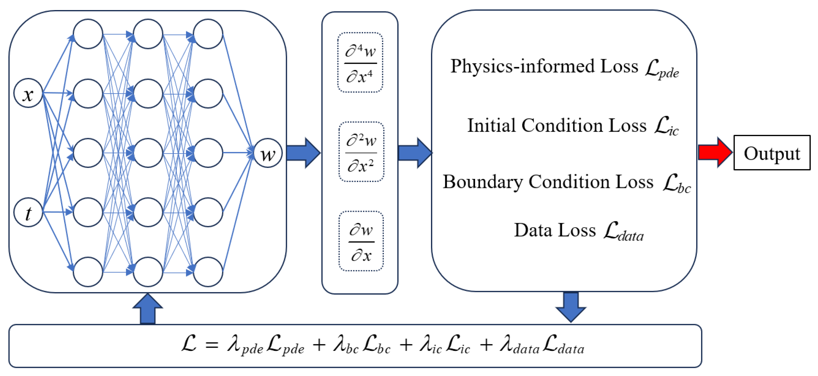
In this study, a physics-informed neural network (PINN) is developed as the primary physics layer. Figure 1 illustrates the architecture of the proposed PINN. The PINN approximates the deflection field w(x,t) using a neural network and incorporates the governing equation, boundary conditions, initial condition, and limited monitoring data established in Section 2 into a unified loss function. Here, ‘physics-informed’ indicates that the network is trained under explicit equilibrium, boundary, and initial constraints embedded in the loss, rather than being a pure data-fit model. The time-dependent coefficients (e.g., E_eff(t)) are provided by established constitutive relations, improving interpretability and reducing the number of free degrees of freedom. In this manner, long-term camber trends can be predicted under “strong physics constraints with sparse data”.

A multilayer feedforward fully connected network is employed to approximate the deflection response:

$$\widehat{w}(x,t)={\mathcal{N}}_{\theta }(f(x,t))$$

(10)

where $\theta$ denotes the network parameters, and $f(x,t)$ is the constructed input feature vector. In this work, a multilayer perceptron (MLP) with four hidden layers is adopted, with the numbers of neurons set to [64, 128, 64, 32]. The hyperbolic tangent ($\mathrm{t}\mathrm{a}\mathrm{n}\mathrm{h}$) is used as the activation function. To enhance training stability, Xavier initialization is adopted for the network weights, and the biases are initialized to zero. The network output is a scalar deflection $\widehat{w}(x,t)$.

Based on the time-dependent beam equation established in Section 2, the PDE residual of the PINN is defined as

$$\mathcal{R}(x,t)=-E_{\mathrm{eff}}(t)I{\displaystyle \frac{{\partial }^4\widehat{w}(x,t)}{\partial x^4}}+q_{\mathrm{g}}+q_{\mathrm{q}}(t)+q_{\mathrm{ps}}(x,t)$$

(11)

A quasi-static assumption is adopted, i.e., for any fixed t, the beam satisfies static bending equilibrium. The fourth-order spatial derivative of the deflection, ${\partial }^4\widehat{w}/\partial x^4$, is computed via automatic differentiation to ensure the differentiability and numerical consistency of the PDE constraint. Although we denote w(x,t), the governing constraint is quasi-static; t serves as a parameter that drives E_eff(t), q(t), and q_ps(x,t). The PINN enforces equilibrium for a family of quasi-static problems across t. To improve numerical conditioning, an appropriate scaling is applied to the PDE residual to enhance training stability. The scaling is also introduced to ensure unit-format consistency by converting the PDE residual into a dimensionless form for loss evaluation.

The primary PINN model is trained using a composite loss function consisting of the physics constraint, boundary conditions, initial condition, and monitoring data:

$$\mathcal{L}={\lambda }_{\mathrm{pde}}{\mathcal{L}}_{\mathrm{pde}}+{\lambda }_{\mathrm{bc}}{\mathcal{L}}_{\mathrm{bc}}+{\lambda }_{\mathrm{ic}}{\mathcal{L}}_{\mathrm{ic}}+{\lambda }_{\mathrm{data}}{\mathcal{L}}_{\mathrm{data}}$$

(12)

$${\mathcal{L}}_{\mathrm{pde}}={\displaystyle \frac{1}{N_{\mathrm{f}}}}\sum _{i=1}^{N_{\mathrm{f}}}{\left|\mathcal{R}(x_i,t_i)\right|}^2$$

(13)

$${\mathcal{L}}_{\mathrm{bc}}={\displaystyle \frac{1}{N_{\mathrm{b}}}\sum _{\mathrm{j}=1}^{N_{\mathrm{b}}}}\left(|\widehat{w}(0,t_{\mathrm{j}}){|}^2+|\widehat{w}(L,t_{\mathrm{j}}){|}^2\right)$$

(14)

$${\mathcal{L}}_{\mathrm{ic}}={\displaystyle \frac{1}{N_0}\sum _{\mathrm{k}=1}^{N_0}}|\widehat{w}(x_{\mathrm{k}},0){|}^2$$

(15)

$${\mathcal{L}}_{\mathrm{data}}={\displaystyle \frac{1}{N_{\mathrm{d}}}\sum _{\mathrm{m}=1}^{N_{\mathrm{d}}}}|\widehat{w}(x_{\mathrm{mid}},t_{\mathrm{m}})-w_{\mathrm{obs}}(t_{\mathrm{m}}){|}^2$$

(16)

The network is trained using the Adam optimizer for 15,000 epochs with an initial learning rate of 1 × 10⁻³ (weight decay 1 × 10⁻⁶). A stepwise learning-rate decay (StepLR, step size 2000, γ = 0.8) is adopted to improve convergence stability. In the PINN training, N_f = 3000 collocation points are used for the PDE residual. The time coordinate is stratified across the three construction stages, while x is sampled uniformly along the span. For boundary constraints, N_b = 500 points are generated at x = 0 and x = L with random times. For the initial condition, N₀ = 500 points are sampled along the span at t = 0. In this study, simply supported displacement conditions are adopted as the primary boundary constraints, and t = 0 is treated as the reference state of the monitoring time axis to characterize subsequent long-term deformation evolution. The monitoring-data term uses midspan deflection observations to calibrate and correct the overall trend.

3.2. Modeling of Additional-Effect Correction

After the constructed primary PINN model converges during training, the predicted deflection at the midspan location $x_{\mathrm{mid}}=L/2$ can be obtained for any time t, denoted as ${\widehat{w}}_{\mathrm{PINN}}(t)$. In addition to the effects of empirical creep–shrinkage and prestress losses on the actual camber, there remain additional influences from unmodeled factors such as model-form errors, high-frequency environmental fluctuations, and thermal effects. By comparing the PINN prediction with the monitored midspan deflection $w_{\mathrm{obs}}(t)$, the additional effect can be defined as

$$w_{\mathrm{r}}(t)=w_{\mathrm{obs}}(t)-{\widehat{w}}_{\mathrm{PINN}}(t)$$

(17)

Under the design assumption that the primary PINN captures the dominant low-frequency physics-driven trend to a sufficient extent, a small-amplitude correction model driven by environmental variables is established within the range of the additional effect. This correction aims to make the final prediction closer to the measured camber while remaining physically bounded and without altering the overall trend. This decomposition is intentionally problem-oriented rather than purely algorithm-driven. In the present application, the primary objective of the residual learner is not to reconstruct the entire camber evolution in an end-to-end manner, but to provide a controlled correction to the discrepancy that remains after the dominant physics-consistent trend has been extracted by the PINN. Such a design is particularly suitable for sparse-monitoring bridge scenarios, where the main long-term response is governed by relatively smooth mechanism-based evolution, whereas the remaining deviations are typically lower-dimensional, monitoring-correlated, and more amenable to structured residual learning. The explicit expression for the final prediction is

$$w_{\mathrm{final}}(t)={\widehat{w}}_{\mathrm{PINN}}(t)+{\widehat{w}}_{\mathrm{r}}(t)$$

(18)

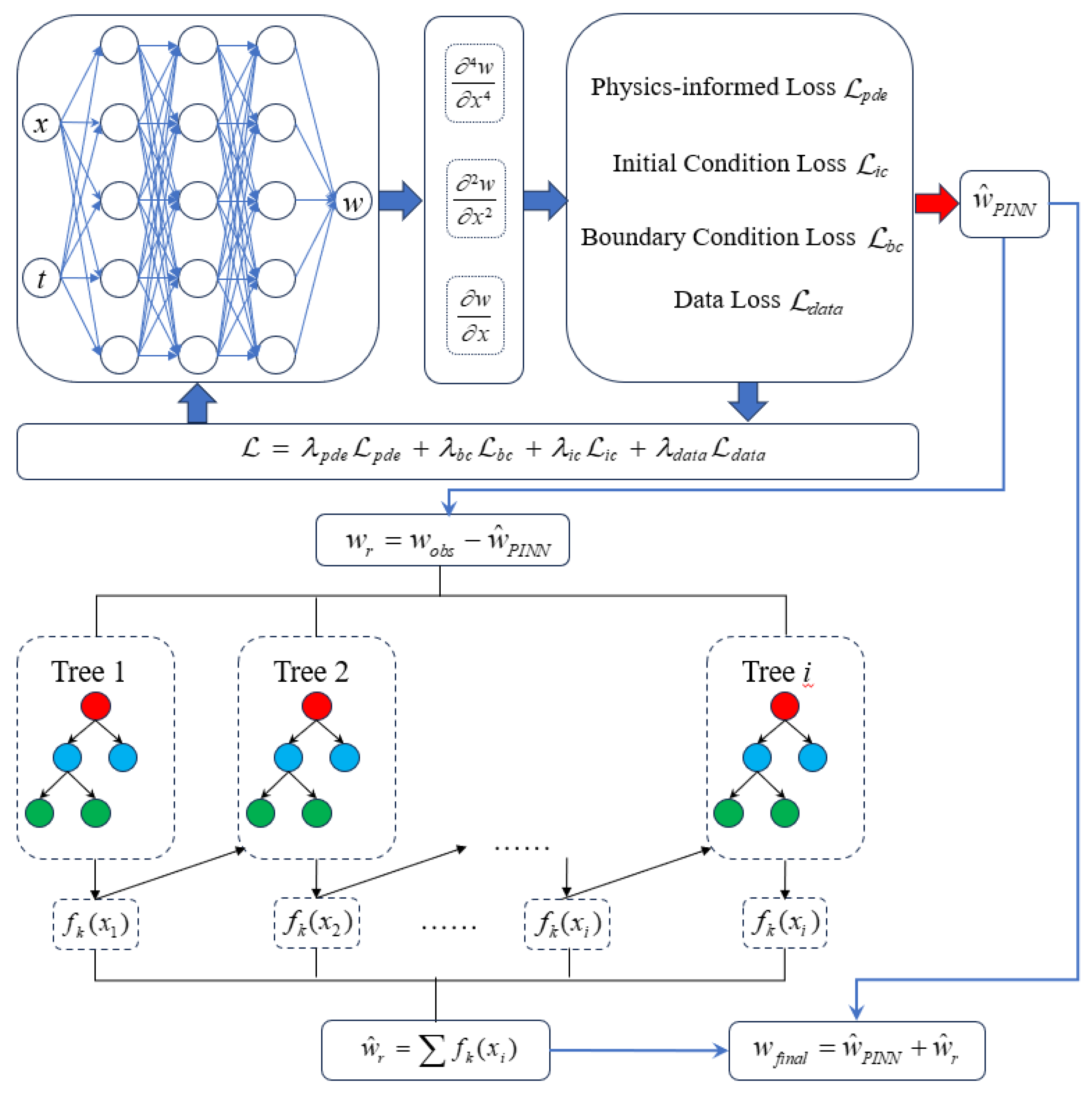
For the choice of the regression model, the gradient boosting tree algorithm XGBoost (eXtreme Gradient Boosting) is adopted as the residual learner. The overall architecture of the model after adding the residual learner is shown in Figure 2. Compared with deep neural networks, XGBoost typically requires fewer samples, is less sensitive to feature scaling and distributions, and can provide stable performance for structured small-sample regression problems. In addition, it offers fast training and relatively interpretable hyperparameters. The regression model can be written as

$${\widehat{w}}_{\mathrm{r}}(t)=f_{\mathrm{XGB}}\left(z(t);\mathit{\beta }\right)$$

(19)

where $\mathit{\beta }$ denotes the tree-model parameters determined through training. In this study, the XGBoost residual learner is configured with n_estimators = 400, max_depth = 3, learning_rate = 0.05, subsample = 0.8, and colsample_bytree = 0.8, with L2 regularization reg_lambda = 1.0. During training, the time instants with measured deflection are selected to form the sample set. The residual mean squared error ${\mathcal{L}}_{\mathrm{res}}$ is used as the objective function, and a train–validation split in the time domain is employed to evaluate model performance. The ${\mathcal{L}}_{\mathrm{res}}$ is expressed as:

$${\mathcal{L}}_{\mathrm{res}}={\displaystyle \frac{1}{N_{\mathrm{d}}}\sum _{i=1}^{N_{\mathrm{d}}}}{\left(r(t_i)-\widehat{r}(t_i)\right)}^2$$

(20)

4. Experiments and Data

4.1. Test Preparation

In this experiment, a 42.5-grade low-alkali ordinary Portland cement was used as the binder. The coarse aggregate consisted of continuously graded crushed stone, with the particle size ranges of 5–10 mm for the small fraction and 10–20 mm for the medium fraction. To improve the workability of the fresh mix and the later-age performance, fly ash was incorporated into the binder at a dosage of 3.7%, and the fine aggregate content was 28%.

To obtain concrete material properties under the same conditions as those of the test beam, a batch of standard concrete specimens was cast simultaneously with the beam using 150 mm × 150 mm × 150 mm cube molds. The specimens were cured under the same environmental conditions as the test beam (same-condition curing). Material tests, including compressive strength, were conducted on the day of beam loading. The measured concrete material properties are listed in

Table 1. Mechanical properties of concrete.

Curing Condition	Age	Average Cube Compressive Strength (MPa)	Elastic Modulus (MPa)
Natural curing	12 d	45.4	3.37 × 104
	20 d	54.2	3.52 × 104
	28 d	54.2	3.52 × 104
	30 d after final stressing	58.6	3.58 × 104
	60 d after final stressing	58.2	3.58 × 104

.

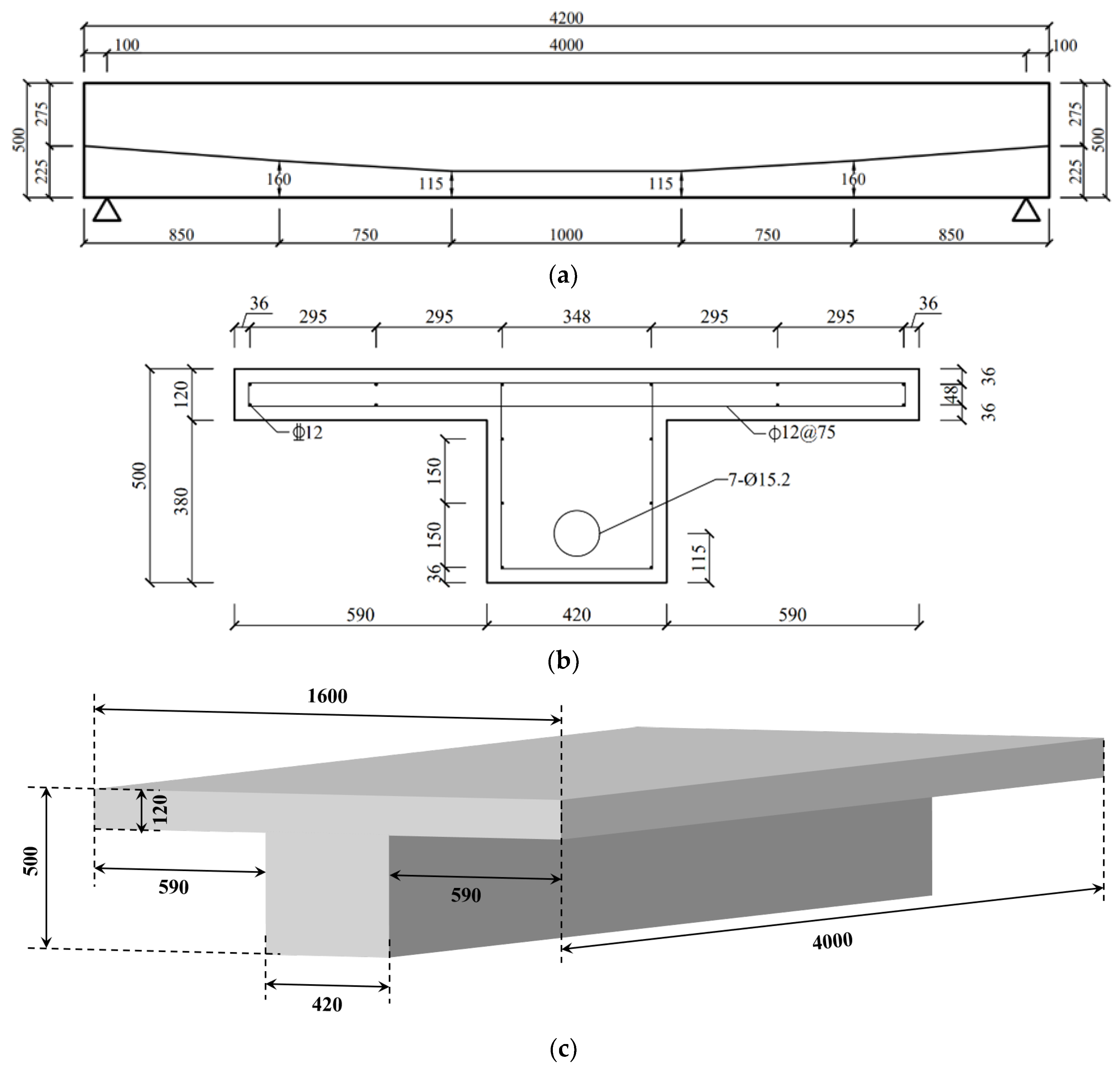
The test program adopted a 24 m-span post-tensioned prestressed concrete (PC) simply supported box girder for a 350 km/h high-speed railway prefabricated ballastless track system as the prototype. The model girder was designed according to similarity theory, with a geometric scale factor of 1:4. The structural dimensions and reinforcement details of the test girder are shown in Figure 3. The designed tendon layout and the locations of the selected control points are shown in Figure 3a. To investigate the effects of key construction and service parameters on the long-term deformation response of the girder, comparative tests were conducted by varying the following factors: the age at final stressing, the control stress at final stressing, the loading age of the secondary permanent load, and the curing regime. The parameter combinations for each specimen are summarized in

Table 2. Design parameters of the test girders.

Specimen ID	Age at Initial Stressing	Control Stress at Initial Stressing	Age at Final Stressing	Control Stress at Final Stressing	Loading Age of the Secondary Permanent Load
PC1	12 d	0.4 fpk	28 d	0.73 fpk	60 d
PC2	12 d	0.4 fpk	20 d	0.65 fpk	60 d
PC3	12 d	0.4 fpk	20 d	0.73 fpk	60 d
PC4	12 d	0.4 fpk	20 d	0.73 fpk	30 d
PC5	12 d	0.4 fpk	20 d	0.73 fpk	90 d

. All specimens were cured under natural curing conditions. High-strength low-relaxation prestressing strands were used, specified as 15.2 mm seven-wire strands (7-ϕ15.2), with a nominal diameter of 15.2 mm, nominal cross-sectional area of 140 mm², elastic modulus of 1.95 × 10⁵ MPa, and ultimate tensile strength grade of 1860 MPa. The prestressing ducts were formed using 70 mm diameter corrugated ducts, and their spatial positions were ensured by coordinating with positioning mesh reinforcement. For conventional reinforcement, 12 mm diameter HRB400 bars were used as longitudinal load-carrying reinforcement, and 12 mm diameter HPB300 bars were used as stirrups. Prestress was applied using the post-tensioning method. The secondary permanent load was simulated by uniformly stacking plain concrete blocks, corresponding to an equivalent line load of 20.216 kN/m for the model girder.

4.2. Experimental Procedure

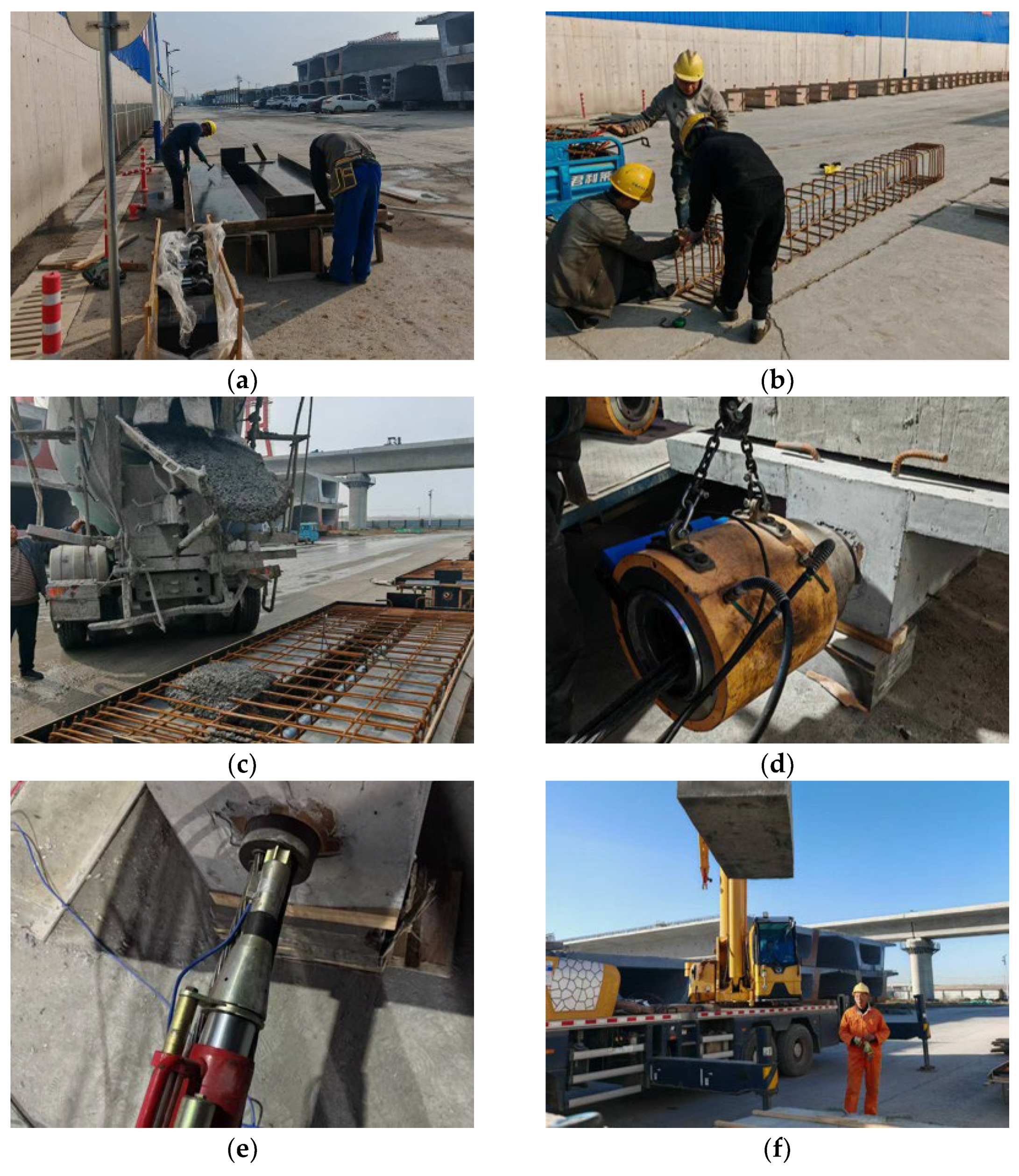
The scaled girder specimens were fabricated using timber formwork. The formwork fabrication procedure is shown in Figure 4a. To reduce formwork deformation during concrete casting, temporary supports made of timber studs were installed on the exterior side of the formwork. For components requiring reserved openings/embedded parts, positioning mesh reinforcement was used to fix their locations inside the formwork, and their positions and stability were rechecked prior to casting. Before pouring, the inner surfaces of the formwork were cleaned and uniformly coated with a release agent to ensure proper concrete forming quality and demolding performance.

The reinforcement cage was assembled by tying, as illustrated in Figure 3, and the tying process is shown in Figure 4b. The completed reinforcement cage was placed integrally into the prepared timber formwork, and the metal corrugated ducts were threaded through the reserved holes in the positioning mesh. Ready-mixed concrete was supplied for casting. The concrete casting process is shown in Figure 4c. During placement, an internal vibrator was used for adequate compaction to ensure concrete densification and to avoid under-vibration or over-vibration. After casting, the top surface of the girder was screeded and finished, and the specimen was covered with felt for curing until the age for initial stressing was reached, at which point prestressing was carried out.

Prestress in the girder specimens was applied using the post-tensioning method, with single-end stressing. After curing, the strands were installed and initial stressing was conducted. The prestressing procedure is shown in Figure 4d–f. Prior to stressing, one end of the strand was fitted through a through-hole (center-hole) load cell, and the procedure was performed in accordance with standard requirements for the full sequence of prestressing operations, including stressing, load holding, and anchorage. After initial stressing, the specimen was moved onto the test bed, compensation loads were applied, monitoring instruments were installed, and measurements were initiated. The relevant procedure is shown in Figure 4f. Final stressing procedure was essentially the same as that for initial stressing.

4.3. Monitoring and Data Acquisition

The monitoring program primarily measured the midspan displacement and the ambient temperature and humidity. Ambient temperature and humidity were collected and stored using an automated data acquisition system. Specifically, the sensor data were acquired and archived via a JMWS-1D-M temperature–humidity acquisition module, and a JMTX-2023 DTU cellular communication module was used to enable remote data transmission and acquisition.

Midspan displacement was measured using dial indicators installed at the beam midspan and at the supports. The midspan dial indicator was used to measure the vertical deformation of the beam, while the support dial indicators were used to measure support settlement, which was subsequently employed to correct the midspan deformation. The midspan and support displacements were measured using dial indicators with a resolution of 0.01 mm. After the initial stressing of the test beam, the beam was moved onto the supports, the instruments were installed, and the initial readings were recorded.

Ambient temperature and relative humidity were automatically sampled at a fixed interval of 30 min by the environmental monitoring module. Midspan displacement (camber) was obtained by manual readings using dial indicators. During the early stage, readings were taken once per day; as the magnitude of camber variation gradually decreased, the reading frequency was reduced to once every 2 days or 3 days while maintaining a consistent measurement routine. All time-series records were time-stamped, synchronized, and aligned onto a unified time axis for subsequent analysis.

4.4. Data Analysis

All time-series were first synchronized and aligned to a unified timeline. Because the camber observations were collected manually with a relatively low sampling frequency, the camber dataset contained limited points; therefore, obvious abnormal readings were removed by manual screening based on engineering judgment (e.g., physically implausible jumps inconsistent with the overall trend). The “abnormal characteristics” of the environmental records refer to outliers in the raw temperature and relative-humidity time series. We adopted the interquartile range (IQR) criterion for robust outlier detection. Specifically, for each variable, we computed the first and third quartiles (Q₁, Q₃) and IQR = Q₃ − Q₁. Samples outside the range [Q₁ − 1.5IQR, Q₃ + 1.5IQR] were regarded as outliers and removed (or replaced by the nearest valid values). This IQR-based procedure is distribution-agnostic and robust for field monitoring data. Missing temperature–humidity data were handled as follows: short gaps (≤3 h) were filled using linear interpolation; for longer gaps, we compared the on-site monitoring records with data from a nearby official meteorological station and found negligible discrepancies, and therefore used the meteorological-station records to supplement the missing segments. The cleaned temperature–humidity series were then used for daily aggregation and subsequent model inputs.

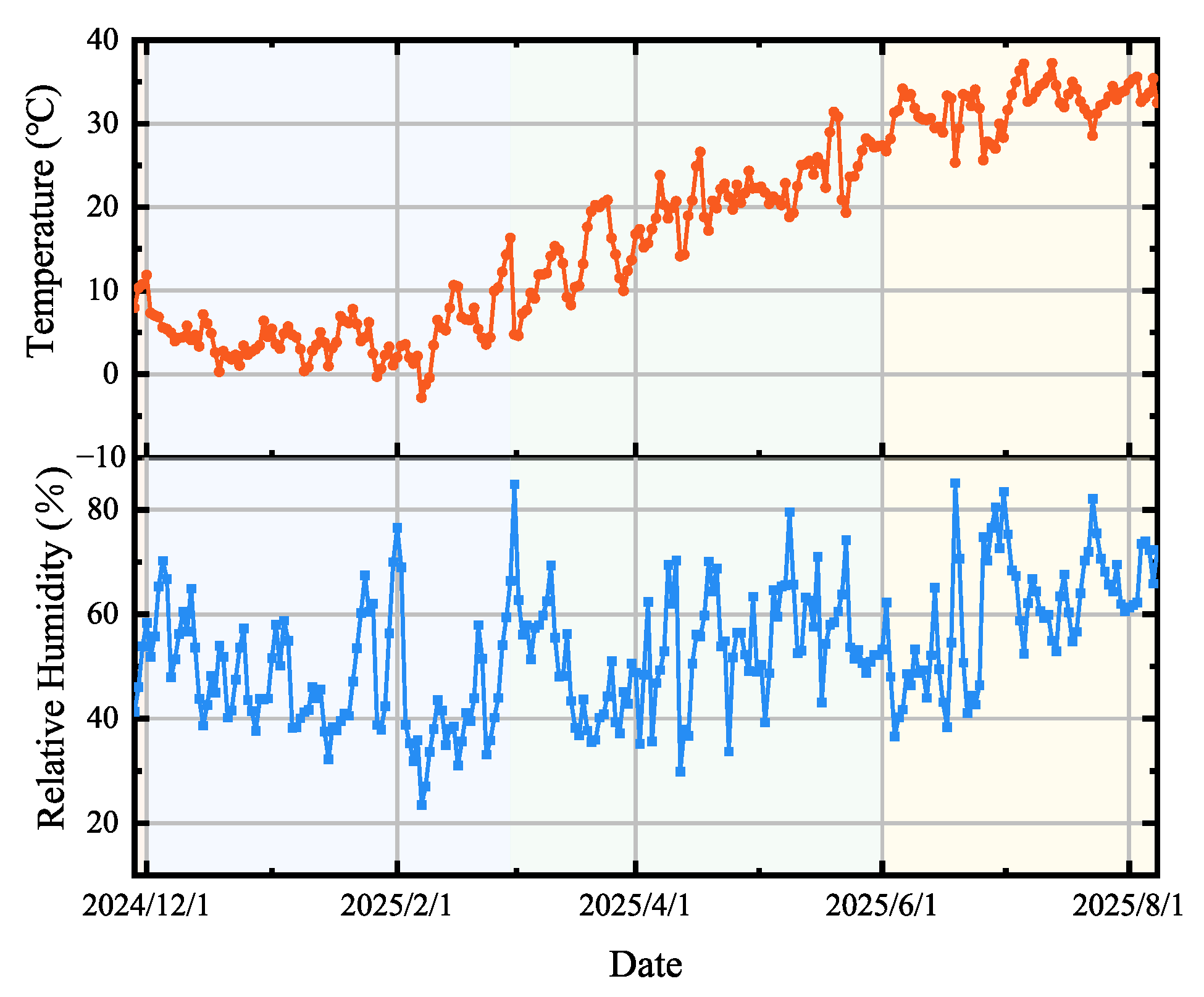
Figure 5 shows the time histories of the average ambient temperature and relative humidity during the monitoring period. As can be observed, both temperature and humidity exhibited periodic variations. The daily average ambient temperature ranged from −5 °C to 35 °C, consistent with local climatic conditions, and the daily relative humidity ranged from 20% to 90%, also consistent with local humidity variations. Such periodic fluctuations in ambient temperature and humidity induced certain high-frequency oscillations and localized turning points in the camber evolution.

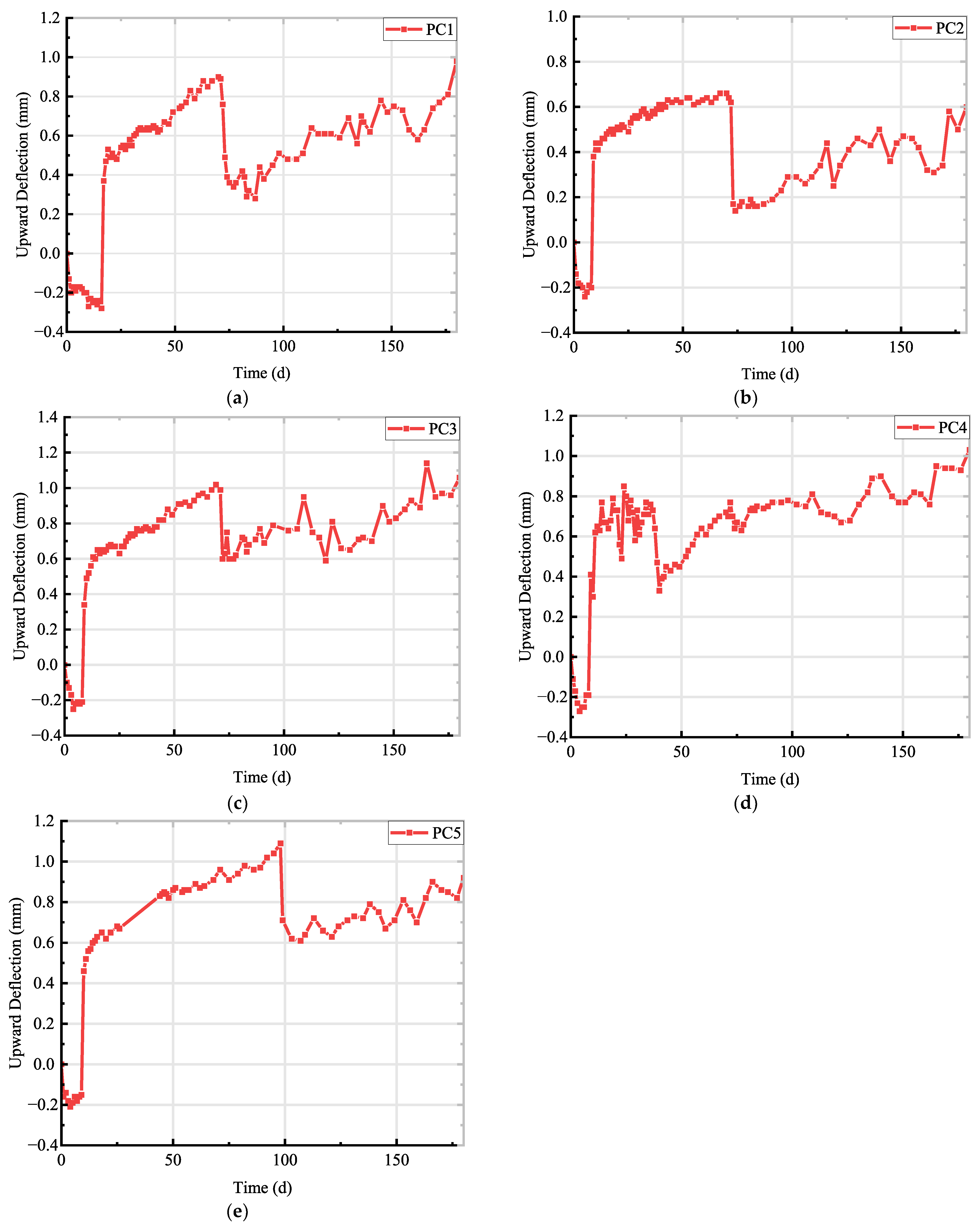
The measured camber evolution obtained from the experiment is shown in Figure 6. It can be clearly observed that the midspan camber of the girder exhibits an overall increasing trend. After the completion of final stressing, the midspan camber shows an abrupt increase, whereas a pronounced abrupt decrease occurs after the application of the secondary permanent load, indicating a significant construction-stage effect.

5. Model Analysis and Results

5.1. Single-Girder Analysis

Based on the overall PINN–XGBoost framework proposed in Section 3, the five scaled test girders obtained in Section 4 are treated as mutually independent objects and modeled separately. As described in Section 4, all test girders share identical geometric dimensions in terms of cross-sectional configuration and span length, whereas they differ in casting time, stressing time, and the time of applying the secondary permanent load. For the i-th girder, denoted as PCi (i = 1, 2, … 5), an individual physics-informed neural network (PINN) is established to approximate the deflection over the span, with the governing equation given in Section 2.

At the PINN level, all girders adopt exactly the same network architecture, input-feature normalization scheme, loss-term weights, and optimizer settings to ensure comparability across specimens. Differences among the test girders are reflected only in:

(1)

their respective key construction time instants (e.g., the time of final stressing and the time when the secondary permanent load is applied);

(2)

their respective prestress levels and loss-related parameters;

(3)

the measured deflection monitoring data.

For each girder, a subset of the monitored time-history data is used to train the PINN by minimizing a loss function that jointly comprises the residual of the governing equation, boundary conditions, initial condition, and the data-misfit term. After completing the single-girder PINN calibration, the difference between the measured deflection and the PINN-predicted deflection is computed at all monitored time instants, yielding a residual sequence. Subsequently, following the method described in Section 3.2, an independent XGBoost residual regression model is trained for each girder using the residuals as outputs and the corresponding environmental features at the same time instants as inputs. In this way, a separately trained PINN-XGBoost hybrid model is obtained for each girder.

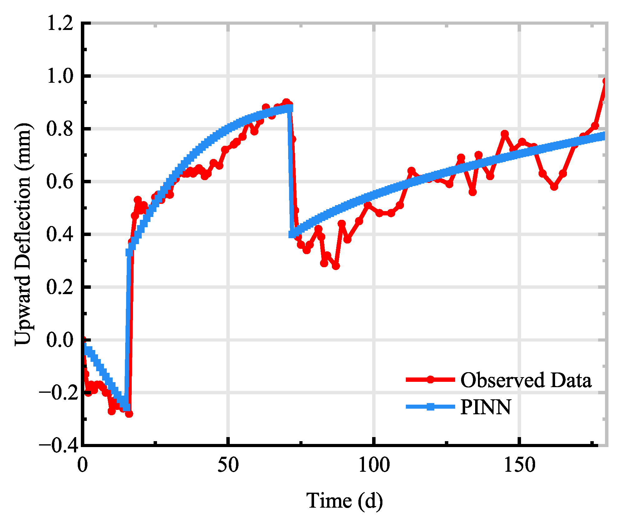
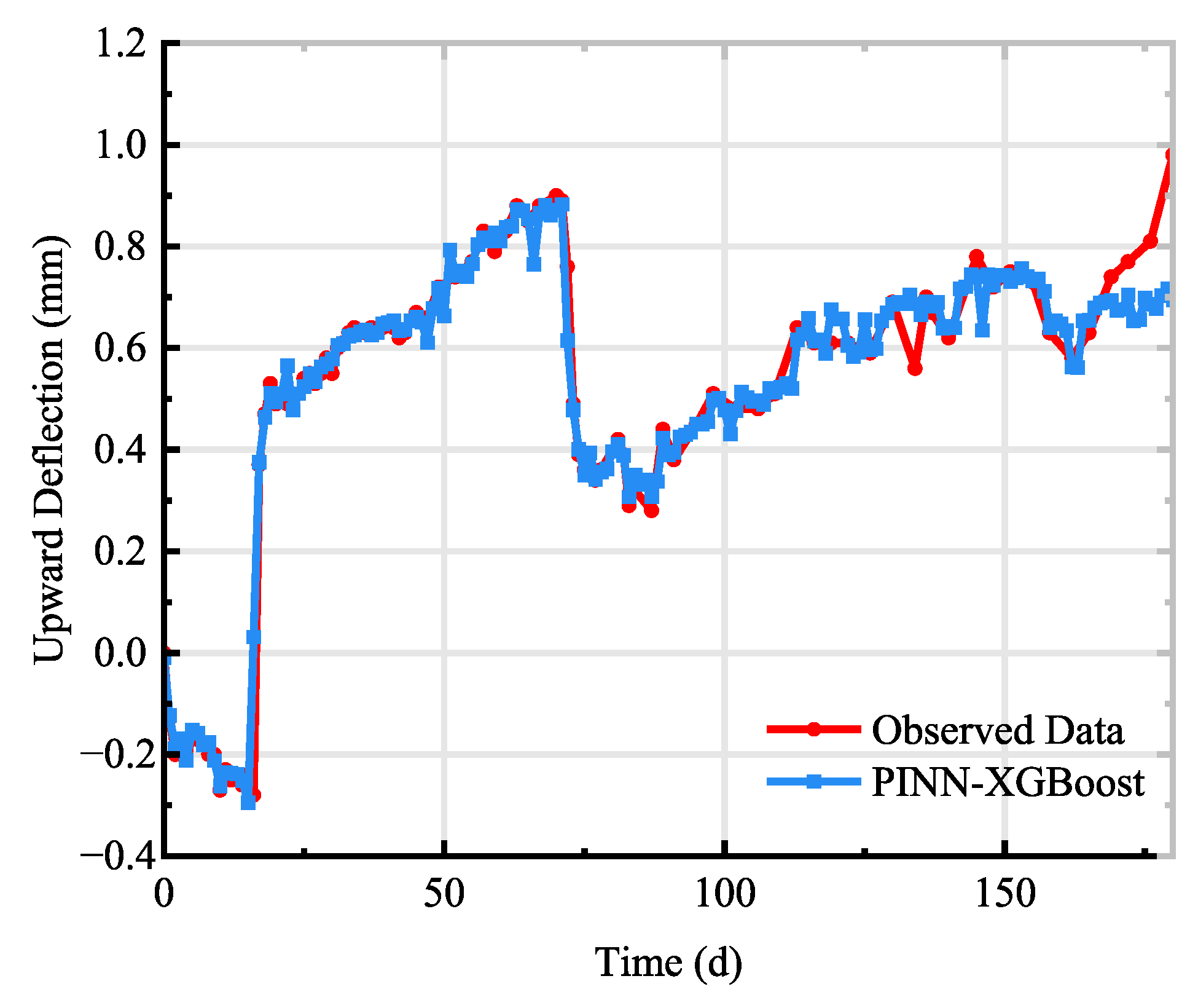
Taking PC1 as an example, the prediction results obtained using the pure PINN framework are shown in Figure 7, and the training and prediction results of the PINN–XGBoost model are shown in Figure 8. As indicated in Figure 7, the pure PINN reproduces the main trend of camber evolution reasonably well, remaining consistent with the measured series while producing a smoother curve. This is consistent with the modeling objective of the PINN, which extracts the low-frequency trend through governing-equation constraints supplemented by monitoring-data calibration.

However, because the primary PINN model does not explicitly incorporate day-to-day fluctuations in ambient temperature and humidity, its capability to track local peaks and valleys, short-period oscillations, and certain stage-wise turning points in the measured curve is relatively limited. This manifests as a “smoother” predicted curve with attenuated local fluctuation amplitudes. Such discrepancies can be interpreted as follows: the PINN layer is primarily responsible for characterizing the physical main trend driven by creep–shrinkage and prestress losses, whereas environmental and other unmodeled effects are delegated to the residual layer.

As shown in Figure 8, after introducing XGBoost-based correction, the agreement between the predicted curve and the measured data improves markedly. The predicted curve becomes closer to the measured series and exhibits richer local variability, indicating that the residual layer effectively compensates for the underfitting of high-frequency disturbances and localized nonlinear details by the primary model. This improvement is consistent with the intended two-layer design, in which the PINN represents the dominant low-frequency trend and the environment-driven residual learner provides a small, controlled compensation for additional effects without altering the overall evolution pattern.

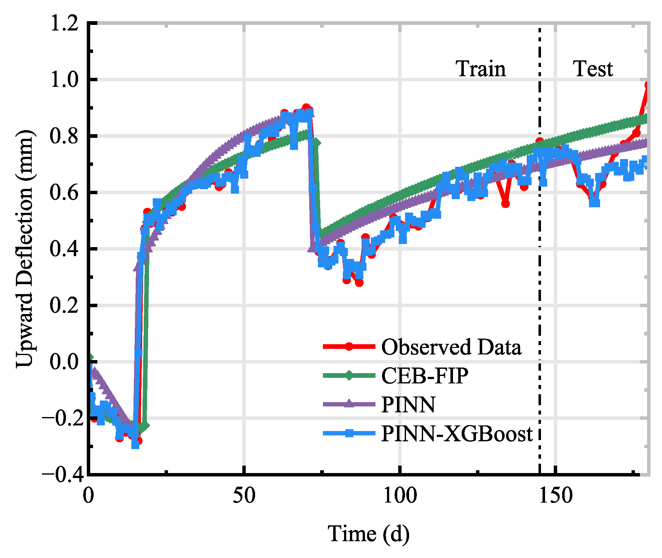
To verify the superiority of the proposed model, a theoretical calculation was performed for girder PC1 based on the CEB-FIP model. The resulting theoretical curve was compared with the predictions from the PINN and the PINN-XGBoost models, as shown in Figure 9. The monitoring time series were split chronologically, where the first 80% of the monitoring period was used for training and the remaining 20% (36 days) was reserved for chronological extrapolation analysis over an unseen future interval. Owing to sparse manual readings and partial missing observations in this stage, this segment was used mainly for trend-consistency assessment rather than as a fully quantified out-of-sample benchmark. The train/test intervals are explicitly marked in the prediction figures. The PINN and the residual learner were trained using training-interval data only. Residuals for XGBoost training were computed only within the training interval, and preprocessing used training-only statistics. As can be observed from Figure 9, all three approaches provide a reasonable overall evolution trend of the midspan camber: the camber gradually develops before and after the completion of final stressing and continues to evolve in the subsequent stage, followed by a pronounced response jump after the time of applying the secondary permanent load. The theoretical calculation captures the overall development trend to some extent; however, because it relies on empirical creep-shrinkage-related losses and typically substitutes specimen-specific material and environmental conditions with average representations, it cannot fully reflect the actual response of an individual girder under natural curing and periodic temperature–humidity fluctuations. Consequently, stage-wise bias accumulation may occur at the single-girder level, leading to more noticeable deviations from the measured values during certain time intervals.

In contrast, by embedding the governing equation into the learning process and calibrating parameters and responses using monitoring data, the PINN can achieve predictions that are closer to measurements under physically consistent constraints. While maintaining the same overall trend and the locations of stage-wise response jumps as the PINN, the PINN-XGBoost model exhibits a stronger capability to track local fluctuations in the measured curve, and its overall agreement is superior to that of the standalone PINN. Moreover, PINN-XGBoost explicitly separates additional influences that are difficult to represent within the physics-based model (e.g., model-form errors, high-frequency environmental fluctuations, and thermal effects) from the main trend and compensates for them in a controlled manner, thereby further improving the agreement over the entire monitoring period.

In summary, under the setting of independent single-girder modeling, the pure PINN can stably extract the physics-driven main trend of long-term camber while preserving prediction smoothness. After incorporating XGBoost-based residual correction using temperature–humidity anomaly features, the proposed hybrid model can effectively compensate for biases caused by environmental and other unmodeled factors without undermining the physical plausibility of the main trend, leading to further improvements in both local-detail fidelity and overall error control.

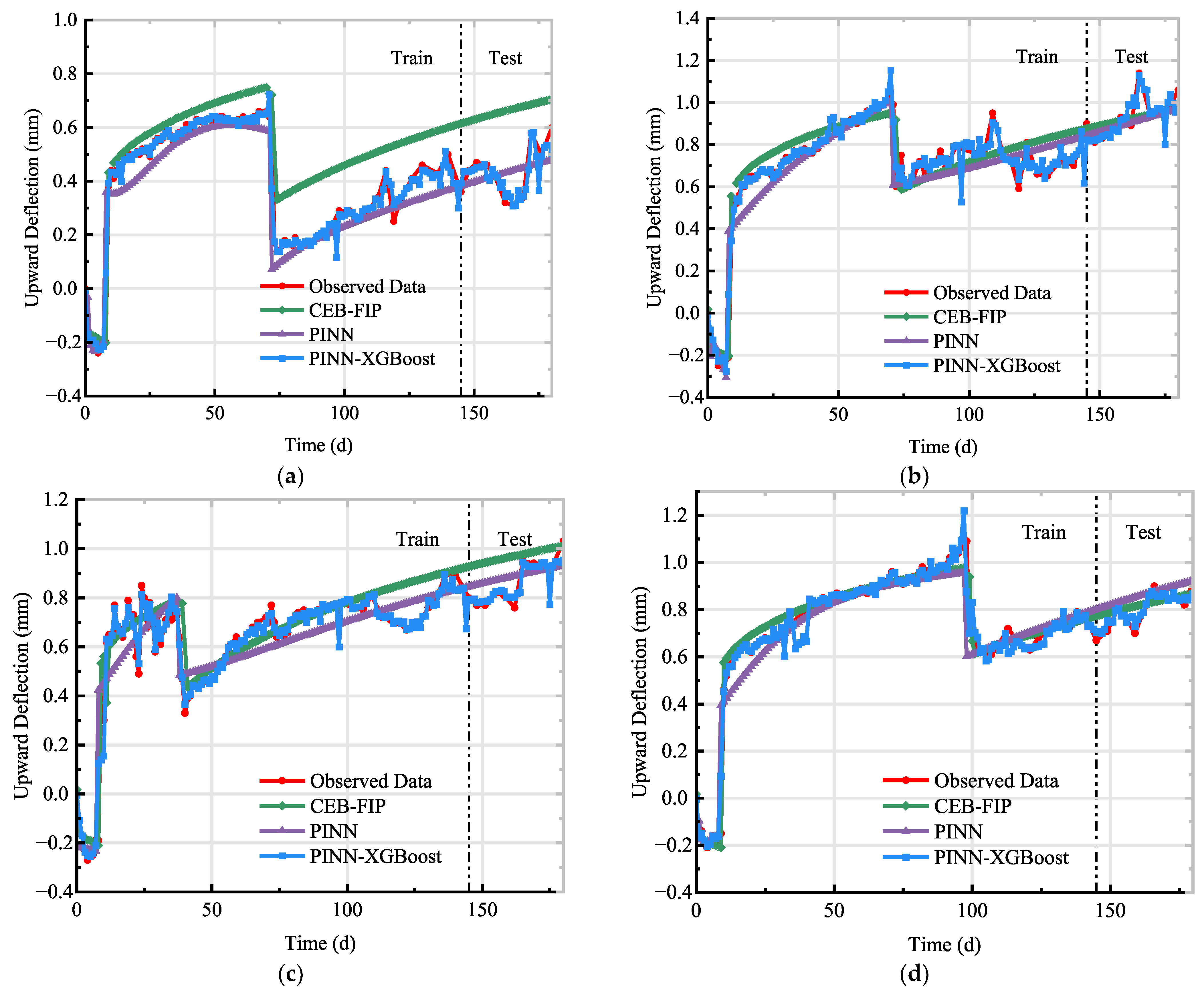
To examine the applicability of the proposed framework to other girders, the same framework was applied to additional scaled girders of the same girder type but with different design parameters. The predicted camber histories obtained by the multiple models for each scaled girder are shown in Figure 10. As indicated in Figure 9 and Figure 10, the PINN–XGBoost workflow shows a qualitatively similar pattern across the independently calibrated girders, i.e., the PINN captures the main trend, whereas the residual learner provides limited compensation for local monitoring-level discrepancies.

For the predictions of PC2–PC5, the pure PINN remains largely consistent with the measured curves in terms of the long-term evolution trend and produces smoother outputs. On this basis, after incorporating XGBoost correction driven by environmental features, the hybrid model yields predictions that are closer to the measured data for each girder. Within the present dataset and under independent single-girder calibration, this result indicates that the two-layer decomposition into the main trend and additional effects can improve agreement with the observed data.

Regarding the theoretical calculation, Figure 10 clearly shows that, because noticeable differences exist among girders, the theoretical model exhibits varying degrees of bias in single-girder predictions. By contrast, the PINN and PINN–XGBoost models can “assimilate and calibrate” each individual girder using monitoring data. This repeated good performance across the independently calibrated girders supports the practical applicability of the proposed workflow in multi-girder monitoring scenarios.

As indicated in Figure 9 and Figure 10, the model using only the physics-informed neural network (PINN) yields camber time-history curves with trends comparable to those measured in monitoring, while producing smoother predictions. After further introducing XGBoost-based residual correction driven by environmental parameters, the PINN–XGBoost model achieves closer agreement with the measured values for each girder in the present dataset. This repeated pattern across the independently calibrated girders indicates that the proposed two-layer decomposition remains practically effective under varied construction-condition combinations within the present dataset. More specifically, the PINN consistently captures the physics-dominated main trend, whereas the residual learner provides limited monitoring-level correction associated with environmental and other unmodeled effects. It should be emphasized that the present validation is performed under independent girder-wise calibration rather than cross-specimen transfer learning. Therefore, the consistency observed across girders should be interpreted as evidence of workflow applicability in a monitoring-oriented setting, rather than proof of strict predictive generalization or transferable inter-specimen modeling.

5.2. Model Evaluation

To evaluate model performance in a transparent manner, metrics are required to describe fitting quality and error characteristics from different perspectives. Because the available monitoring data are limited and the later extrapolation stage contains sparse manual readings with partial missing observations, the quantitative metrics reported in this study are focused on the first 80% of the monitoring history. Specifically, the coefficient of determination (R²), mean absolute error (MAE), and root mean squared error (RMSE) are adopted as the primary criteria. These three metrics reflect explained variance, average absolute error, and sensitivity to larger deviations, respectively, and are therefore used to assess model performance within the observed data interval available for quantitative comparison. For the remaining 20% future interval, the analysis is presented primarily as chronological extrapolation with qualitative trend comparison, rather than as a strict statistical benchmark.

The coefficient of determination (R²) quantifies the extent to which the model explains the variance of the target variable. Values closer to 1 indicate better agreement with the data. The mean absolute error (MAE) is the mean of the absolute differences between predictions and observations, which directly reflects the average error magnitude and is less sensitive to outliers, making it suitable for characterizing typical error levels. A smaller MAE indicates higher predictive accuracy. The root mean squared error (RMSE) is computed as the square root of the mean of squared differences between predictions and observations and reflects the overall error level; because it assigns a higher penalty to larger errors, it is more sensitive to outliers. A smaller RMSE indicates better predictive performance. The formulas for R², RMSE, and MAE are given as follows:

$$R^2=1-{\displaystyle \frac{{\displaystyle \sum _{i=1}^n{(y_i-{\widehat{y}}_i)}^2}}{{\displaystyle \sum _{i=1}^n{(y_i-\overline{y})}^2}}}$$

(21)

$$MAE={\displaystyle \frac{1}{n}}\sum _{i=1}^n\left|{\widehat{y}}_i-y_i\right|$$

(22)

$$RMSE=\sqrt{{\displaystyle \frac{{\displaystyle \sum _{i=1}^n{(y_i-{\widehat{y}}_i)}^2}}{n}}}$$

(23)

where $y_i$ and ${\widehat{y}}_i$ denote the measured (ground-truth) value and the predicted value of the i-th sample, respectively; $\overline{y}$ is the mean of the measured values; and n is the number of samples.

Table 3. Quantitative evaluation metrics of different models over the first 80% of the monitoring history.

Girder	Model	R2	MAE	RMSE
PC1	PINN	0.954	0.063	0.084
	PINN-XGBoost	0.976	0.023	0.053
	Theoretical calculation	0.856	0.077	0.129
PC2	PINN	0.920	0.055	0.066
	PINN-XGBoost	0.980	0.015	0.033
	Theoretical calculation	0.680	0.108	0.136
PC3	PINN	0.928	0.059	0.078
	PINN-XGBoost	0.989	0.018	0.030
	Theoretical calculation	0.923	0.064	0.085
PC4	PINN	0.885	0.079	0.094
	PINN-XGBoost	0.979	0.021	0.040
	Theoretical calculation	0.890	0.070	0.095
PC5	PINN	0.967	0.046	0.061
	PINN-XGBoost	0.996	0.011	0.020
	Theoretical calculation	0.977	0.036	0.052
Averaged results	PINN	0.931	0.060	0.077
	PINN-XGBoost	0.984	0.018	0.035
	Theoretical calculation	0.865	0.076	0.099

summarizes the evaluation metrics of different models over the first 80% of the monitoring history, where direct quantitative comparison with observed data is available under limited-data conditions. Based on the comparison results for PC1-PC5 in Table 3, the three methods exhibit a clear performance hierarchy in terms of goodness-of-fit (R²) and error metrics (MAE and RMSE). The proposed PINN–XGBoost model consistently achieves the best performance for all girders, with R² stably ranging from 0.976 to 0.996, MAE from 0.011 to 0.023, and RMSE from 0.020 to 0.053, indicating lower fitting and prediction errors within the evaluated monitoring interval. In comparison, the PINN ranks second in overall accuracy, whereas the theoretical calculation shows larger variability.

Averaged over the five girders, PINN–XGBoost attains a mean R² of 0.984, MAE of 0.0176, and RMSE of 0.0352. Relative to the PINN, whose mean R² is 0.9308, the mean R² increases by 0.0532 (approximately a 5.7% relative improvement). Meanwhile, MAE and RMSE decrease by approximately 70.9% and 54.0%, respectively. These results indicate that, on top of the physics-based constraints provided by the PINN, incorporating a residual component to represent additional effects can substantially reduce both systematic deviation and error dispersion within the observed data interval. The consistently good performance across the five girders suggests that the proposed workflow can be calibrated and applied in a stable manner under different construction-condition combinations. However, this should not be interpreted as evidence of cross-specimen transfer generalization, because each girder was modeled independently.

5.3. Interpretation of Model Behavior and Applicability

The improved predictive performance of the hybrid model should not be interpreted simply as the consequence of adding a more flexible regression component. Rather, it arises from a task-consistent decomposition of the prediction problem. In the proposed framework, the PINN is responsible for capturing the low-frequency, mechanism-dominated evolution of camber governed primarily by creep, shrinkage, prestress loss, and stage-dependent loading. Because these effects are embedded through the governing equation and auxiliary constraints, the resulting prediction remains smooth, physically plausible, and consistent with the observed stage-wise response jumps. This explains why the standalone PINN is able to reproduce the overall long-term trend more reliably than the purely theoretical calculation under sparse-monitoring conditions.

By contrast, the residual learner is introduced only after the main trend has been identified and is therefore tasked with compensating the remaining discrepancy between the PINN prediction and the measurements. This discrepancy may arise from model-form simplifications, unmodeled thermal or hygro-environmental effects, local monitoring fluctuations, and other specimen-specific influences that are difficult to encode explicitly in the quasi-static physics layer. In this sense, the role of XGBoost is not to redefine the structural mechanics of camber development, but to provide a bounded correction at the monitoring level. The closer agreement of the PINN–XGBoost model with the measured curves therefore reflects the effectiveness of separating trend-dominated and discrepancy-dominated components, rather than merely increasing model flexibility.

This interpretation also helps clarify the broader applicability of the proposed workflow. Within the present dataset, a qualitatively consistent pattern is observed across the independently calibrated girders: the PINN captures the mechanism-dominated trend, whereas the residual learner provides limited compensation for local deviations. Such repeated behavior supports the practical usefulness of the two-layer workflow for sparse-monitoring bridge applications after girder-wise calibration. The current results should be understood as evidence that the proposed decomposition remains effective across multiple girders with different construction-condition combinations under the same overall modeling philosophy.

A further implication is that uncertainty quantification and transferability remain open methodological extensions rather than completed components of the present study. The current framework is deterministic and is intended primarily to improve long-term trend prediction and monitoring-level agreement under limited observations. Future work should therefore examine uncertainty-aware formulations, more explicit thermo-hygro-mechanical coupling when richer environmental observations are available, and cross-girder transfer strategies under limited calibration data.

5.4. Practical Limitations and Deployment Considerations

The proposed framework is developed on an Euler–Bernoulli beam-based governing equation and validated on scaled simply supported girders. Extension to full-scale bridges is a plausible next step, but it will require additional modeling and validation to account for system-level effects beyond the present scaled-girder setting. Nevertheless, full-scale deployment may require additional modeling components to account for system-level effects (multi-girder interaction, continuous-span constraints, bearing/slab restraints, and temperature gradients). In such cases, the physics layer can be upgraded (e.g., refined beam theory or multi-span constraints) while retaining the same “physics backbone + residual correction” architecture. Training a PINN is more expensive than fitting a purely data-driven regressor because it enforces PDE residuals through automatic differentiation. After training, online inference is fast (a forward pass), and the residual learner (XGBoost) is lightweight.

The physics layer is designed to operate under sparse monitoring because the governing equation, boundary/initial conditions, and staged loading history provide strong constraints. For reliable deployment, at minimum, the system should collect midspan deflection (with support readings if settlement correction is needed) and ambient temperature–humidity records synchronized in time. In our setup, the displacement sensor resolution is 0.01 mm, and the residual correction is used as a bounded small-amplitude compensation rather than altering the physics-driven trend.

However, the approach may degrade when (i) monitoring data are corrupted (sensor drift, bias, or long missing intervals), (ii) boundary conditions or structural state change abruptly (bearing slip, unexpected settlement, damage), or (iii) environmental/loading conditions fall outside the training distribution, in which case the residual learner may extrapolate unreliably. Practical mitigation includes data-quality screening, monitoring the residual statistics as an alarm indicator, bounding the correction magnitude, and periodically re-calibrating/retraining the model when a persistent distribution shift is detected.

6. Conclusions

Building on established hybrid physics–data modeling and discrepancy-correction paradigms, this study developed a monitoring-oriented workflow for long-term midspan camber prediction of prestressed concrete girders under small-sample conditions. First, an Euler–Bernoulli beam–based mechanical framework is established, where key time-dependent mechanisms—including creep, shrinkage, and prestress losses—are incorporated into the governing equation and embedded into the PINN loss function to learn the main camber trend. Subsequently, additional influences that are difficult to explicitly represent in the physics-based model, such as daily temperature–humidity fluctuations, are aggregated and compensated at the measurement-discrepancy level via a gradient boosting tree residual learner. In this way, long-term prediction accuracy is improved while maintaining physical consistency. The main conclusions are as follows:

(1)

A stage-aware physics-informed prediction framework tailored to long-term camber prediction was developed. Creep–shrinkage representations and the effective modulus method were adopted to capture age-dependent stiffness evolution. Together with instantaneous loss, relaxation loss, and creep–shrinkage-induced losses, the effective prestress was determined, yielding a time-dependent beam governing equation with an associated set of boundary and initial conditions that can be directly incorporated into the PINN to provide a physics-consistent basis for learning the dominant low-frequency camber trend.

(2)

A hybrid prediction strategy based on a two-layer decomposition into a mechanism-dominated main trend and a measurement-level discrepancy was proposed, resulting in the PINN–XGBoost model. After the primary PINN captures the overall camber evolution, the difference between measurements and PINN predictions is defined as the additional effect and is predicted using XGBoost. The hybrid model provides limited discrepancy compensation without overriding the underlying physical trend, thereby improving predictive accuracy.

(3)

Comparative results across the five independently calibrated girders indicate that the proposed hybrid workflow is effective for practical monitoring-oriented camber prediction under the present engineering measurement setting. For each girder, the PINN–XGBoost model achieves closer agreement with the observed data than the standalone PINN and the theoretical calculation within the evaluated monitoring interval, with R² ranging from 0.976 to 0.996, MAE from 0.011 to 0.023, and RMSE from 0.020 to 0.053 over the first 80% of the monitoring history. The repeated good predictive performance across different girders supports the engineering applicability of the proposed method in multi-girder monitoring scenarios with sparse measurements and periodic environmental fluctuations. However, this effectiveness is demonstrated under independent girder-wise calibration and should not be interpreted as evidence of formal cross-specimen transferability or strict predictive generalization.

Overall, the contribution of the proposed workflow should be understood at the level of a structured, problem-oriented implementation rather than the introduction of a new general hybrid modeling paradigm. Its main value lies in explicitly separating the mechanism-dominated long-term camber trend from the monitoring-level discrepancy and then modeling these two components in a complementary manner. For sparse-monitoring bridge applications, this decomposition is advantageous because it preserves physical plausibility at the trend level while improving local agreement with observations through bounded residual correction. Within the present scaled-specimen dataset, the proposed PINN–XGBoost workflow demonstrates repeated effectiveness across multiple girders after independent girder-wise calibration. The results therefore support its practical applicability for monitoring-oriented long-term camber prediction under varied construction-condition combinations and periodic environmental fluctuations.

This study also has limitations. First, the current validation is based on scaled girders rather than long-term deployment on full-scale in-service bridges. Second, although the monitoring data partially reflect realistic sparse and irregular field-like conditions, the present study does not include dedicated robustness benchmarks such as synthetic noise perturbation, controlled missing-data ablation, or leave-one-girder-out transfer evaluation. Third, the present framework remains deterministic and does not provide uncertainty-aware prediction.

Future research will focus on uncertainty-aware formulations, transferability across girders with limited monitoring data, more explicit thermo-hygro-mechanical coupling when richer environmental observations are available, and validation under full-scale field monitoring conditions.

References

1. Tong, T.; Liu, Z.; Zhang, J.; Yu, Q. Long-Term Performance of Prestressed Concrete Bridges under the Intertwined Effects of Concrete Damage, Static Creep and Traffic-Induced Cyclic Creep. Eng. Struct. 2016, 127, 510–524. [Google Scholar] [CrossRef]
2. Asamoto, S.; Kato, K.; Maki, T. Effect of Creep Induction at an Early Age on Subsequent Prestress Loss and Structural Response of Prestressed Concrete Beam. Constr. Build. Mater. 2014, 70, 158–164. [Google Scholar] [CrossRef]
3. Deng, L.; Yan, W.; Nie, L. A Simple Corrosion Fatigue Design Method for Bridges Considering the Coupled Corrosion-Overloading Effect. Eng. Struct. 2019, 178, 309–317. [Google Scholar] [CrossRef]
4. Shi, Y.; Wang, Y.; Wang, L.-N.; Wang, W.-N.; Yang, T.-Y. Bridge Tower Warning Method Based on Improved Multi-Rate Fusion Under Strong Wind Action. Buildings 2025, 15, 2733. [Google Scholar] [CrossRef]
5. Shi, Y.; Wang, Y.; Wang, L.-N.; Wang, W.-N.; Yang, T.-Y. Bridge Cable Performance Warning Method Based on Temperature and Displacement Monitoring Data. Buildings 2025, 15, 2342. [Google Scholar] [CrossRef]
6. He, Z.; Li, W.; Salehi, H.; Zhang, H.; Zhou, H.; Jiao, P. Integrated Structural Health Monitoring in Bridge Engineering. Autom. Constr. 2022, 136, 104168. [Google Scholar] [CrossRef]
7. Figueiredo, E.; Brownjohn, J. Three Decades of Statistical Pattern Recognition Paradigm for SHM of Bridges. Struct. Health Monit. 2022, 21, 3018–3054. [Google Scholar] [CrossRef]
8. Ji, W.; Li, X.; He, J.; Zhang, X.; Li, J. Research Status of Monitoring, Detection, and Intelligent Identification of Weathering Steel Bridges. J. Constr. Steel Res. 2024, 220, 108814. [Google Scholar] [CrossRef]
9. Hoskere, V.; Hassanlou, D.; Rahman, A.U.; Bazrgary, R.; Ali, M.T. Unified Framework for Digital Twins of Bridges. Autom. Constr. 2025, 175, 106214. [Google Scholar] [CrossRef]
10. FIB. FIB Model Code for Concrete Structures 2010; John Wiley & Sons: Hoboken, NJ, USA, 2013. [Google Scholar]
11. Wendner, R.; Hubler, M.H.; Bažant, Z.P. The B4 Model for Multi-Decade Creep and Shrinkage Prediction. In Proceedings of the Mechanics and Physics of Creep, Shrinkage, and Durability of Concrete, Cambridge, MA, USA, 22–25 September 2013; ASCE: Reston, VA, USA, 2013; pp. 429–436. [Google Scholar]
12. Neville, A. Time Effects in Concrete Structures. Eng. Struct. 1989, 11, 202–203. [Google Scholar] [CrossRef]
13. Park, Y.-S.; Lee, Y.-H. Incremental Model Formulation of Age-Dependent Concrete Character and Its Application. Eng. Struct. 2016, 126, 328–342. [Google Scholar] [CrossRef]
14. Wang, W.; Gong, J. New Relaxation Function and Age-Adjusted Effective Modulus Expressions for Creep Analysis of Concrete Structures. Eng. Struct. 2019, 188, 1–10. [Google Scholar] [CrossRef]
15. Yapar, O.; Basu, P.K.; Nordendale, N. Accurate Finite Element Modeling of Pretensioned Prestressed Concrete Beams. Eng. Struct. 2015, 101, 163–178. [Google Scholar] [CrossRef]
16. Moreira, L.S.; Sousa, J.B.M.; Parente, E. Nonlinear Finite Element Simulation of Unbonded Prestressed Concrete Beams. Eng. Struct. 2018, 170, 167–177. [Google Scholar] [CrossRef]
17. Li, R.; He, Q.; Zhu, S.; Yan, J.; Zhai, W. A New Methodology for Pre-Camber Design of a Long-Span Bridge Considering Dynamic Train Load and Complex Environmental Effects. Eng. Struct. 2024, 302, 117349. [Google Scholar] [CrossRef]
18. Kumar, S.; Nallasivam, K. Modal Analysis of a Prestressed Concrete Box-Girder Bridge Using the Finite Element Technique. J. Vib. Eng. Technol. 2025, 14, 14. [Google Scholar] [CrossRef]
19. Flah, M.; Nunez, I.; Ben Chaabene, W.; Nehdi, M.L. Machine Learning Algorithms in Civil Structural Health Monitoring: A Systematic Review. Arch. Comput. Methods Eng. 2020, 28, 2621–2643. [Google Scholar] [CrossRef]
20. Zhu, S.; Yang, M.; Xiang, T.; Xu, X.; Li, Y. Advanced Time-Series Prediction of Bridge Long-Term Deflection Using the Learning Models. Structures 2024, 67, 106967. [Google Scholar] [CrossRef]
21. Oh, B.K.; Park, H.S.; Glisic, B. Prediction of Long-Term Strain in Concrete Structure Using Convolutional Neural Networks, Air Temperature and Time Stamp of Measurements. Autom. Constr. 2021, 126, 103665. [Google Scholar] [CrossRef]
22. Wang, X.; Xie, G.; Liu, W.; Kong, H.; Gao, Y. A Long-Term Vertical Displacement Prediction Method of Concrete Bridges Based on Meteorological Shared Data and Optimized GRU Model. Measurement 2025, 253, 117811. [Google Scholar] [CrossRef]
23. Chen, Y.; Xie, Q.; Li, Y.; Liang, R.; Zhu, L. A Review of ML for Bridge Vertical Displacement. KSCE J. Civ. Eng. 2026, 30, 100464. [Google Scholar] [CrossRef]
24. Chen, Z.; Ma, M.; Li, T.; Wang, H.; Li, C. Long Sequence Time-Series Forecasting with Deep Learning: A Survey. Inf. Fusion 2023, 97, 101819. [Google Scholar] [CrossRef]
25. Zhang, M.; Guo, T.; Zhang, G.; Liu, Z.; Xu, W. Physics-Informed Deep Learning for Structural Vibration Identification and Its Application on a Benchmark Structure. Philos. Trans. R. Soc. A Math. Phys. Eng. Sci. 2023, 382, 20220400. [Google Scholar] [CrossRef]
26. He, Z.; Huang, T.-L.; Chen, B. Physics-Informed Graph Transformer Network for Predicting Cable-Stayed Bridge Structural Deflection Response. Adv. Eng. Inform. 2026, 69, 103897. [Google Scholar] [CrossRef]
27. Ma, Y.; Zhang, B.; Huang, K.; Wang, L. Probabilistic Prediction and Early Warning for Bridge Bearing Displacement Using Sparse Variational Gaussian Process Regression. Struct. Saf. 2025, 114, 102564. [Google Scholar] [CrossRef]
28. Xu, B.; Liu, C. A Deep Kernel Regression-Based Forecasting Framework for Temperature-Induced Strain in Large-Span Bridges. Eng. Struct. 2025, 323, 119259. [Google Scholar] [CrossRef]
29. Entezami, A.; Behkamal, B.; De Michele, C.; Mariani, S. A Kernelized Deep Regression Method to Simultaneously Predict and Normalize Displacement Responses of Long-Span Bridges via Limited Synthetic Aperture Radar Images. Struct. Health Monit. 2025. [Google Scholar] [CrossRef]
30. Karniadakis, G.E.; Kevrekidis, I.G.; Lu, L.; Perdikaris, P.; Wang, S.; Yang, L. Physics-Informed Machine Learning. Nat. Rev. Phys. 2021, 3, 422–440. [Google Scholar] [CrossRef]
31. Hu, H.; Qi, L.; Chao, X. Physics-Informed Neural Networks (PINN) for Computational Solid Mechanics: Numerical Frameworks and Applications. Thin-Walled Struct. 2024, 205, 112495. [Google Scholar] [CrossRef]
32. Ecemiş, A.S.; Yildizel, S.A.; Beskopylny, A.N.; Stel’makh, S.A.; Shcherban’, E.M.; Aksoylu, C.; Madenci, E.; Özkılıç, Y.O. Sustainable Concrete with Waste Tire Rubber and Recycled Steel Fibers: Experimental Insights and Hybrid PINN-CatBoost Prediction. Polymers 2025, 17, 2910. [Google Scholar] [CrossRef]
33. Mohamud, M.A.; Alasiri, M.R.; Özdöner, N.; Yıldızel, S.A.; Özkılıç, Y.O. Physics-Guided Machine Learning Framework for RCA Concrete by Experimental Database, Modelling, and Statistical Validation. Sci. Rep. 2026, 16, 7907. [Google Scholar] [CrossRef] [PubMed]
34. Özkılıç, Y.O.; Karalar, M.; Alasiri, M.R.; Zeybek, Ö.; Yildizel, S.A. A Hybrid CNN–PINN–NSGA-II Framework for Physics-Consistent Surrogate Modeling of Reinforced Concrete Beams Incorporating Waste Fired Clay. Buildings 2026, 16, 682. [Google Scholar] [CrossRef]
35. Haywood-Alexander, M.; Arcieri, G.; Kamariotis, A.; Chatzi, E. Response Estimation and System Identification of Dynamical Systems via Physics-Informed Neural Networks. Adv. Model. Simul. Eng. Sci. 2025, 12, 8. [Google Scholar] [CrossRef] [PubMed]
36. Liu, J.; Li, Y.; Sun, L.; Wang, Y.; Luo, L. Physics and Data Hybrid-Driven Interpretable Deep Learning for Moving Force Identification. Eng. Struct. 2025, 329, 119801. [Google Scholar] [CrossRef]
37. Wu, Y.; Yin, Z.; Gao, Y.; Yang, S.; Hou, Y. Constitutive Model-Constrained Physics-Informed Neural Networks Framework for Nonlinear Structural Seismic Response Prediction. Comput. Methods Appl. Mech. Eng. 2025, 443, 118079. [Google Scholar] [CrossRef]
38. Teloli, R.d.O.; Tittarelli, R.; Bigot, M.; Coelho, L.; Ramasso, E.; Moal, P.L.; Ouisse, M. A Physics-Informed Neural Networks Framework for Model Parameter Identification of Beam-like Structures. Mech. Syst. Signal Process. 2025, 224, 112189. [Google Scholar] [CrossRef]
39. Wu, T.; Zhu, W.; Tang, L.; Lang, L.; Xu, J.; Yuan, Q.; Zhou, Z. Accurate Structural Displacement Reconstruction from Acceleration and Computer Vision Measurements Using Physics-Informed Neural Networks. Mech. Syst. Signal Process. 2025, 235, 112961. [Google Scholar] [CrossRef]
40. Park, H.-W.; Hwang, J.-H. Predicting the Early-Age Time-Dependent Behaviors of a Prestressed Concrete Beam by Using Physics-Informed Neural Network. Sensors 2023, 23, 6649. [Google Scholar] [CrossRef]
41. Li, X.; Zhang, F.-L.; Xiang, W.; Liu, W.-X.; Fu, S.-J. Structural Health Monitoring System Based on Digital Twins and Real-Time Data-Driven Methods. Structures 2024, 70, 107739. [Google Scholar] [CrossRef]
42. Zhai, G.; Spencer, B.F.; Yan, J.; Liao, W.; Gu, D.; Contiguglia, C.P.; Demartino, C.; Xu, Y. Coupled Data/Physics-Driven Framework for Accurate and Efficient Structural Response Simulation. Eng. Struct. 2024, 327, 119636. [Google Scholar] [CrossRef]
43. Xin, Y.; Cai, Y.-S.; Wang, Z.-C.; Li, J.; Hou, W.-C.; Li, C. Hybrid-Driven Digital Twin Framework for Time-Variant Reliability Assessment of Civil Structures. Struct. Control Health Monit. 2025, 2025, 1167999. [Google Scholar] [CrossRef]
44. Kang, C.; Walker, M.; Bartels, J.-H.; Marzahn, G.; Marx, S. Digital Twin Technologies for Bridge Lifecycle Management-Literature Insights and a Pilot Study on the Nibelungen Bridge. Results Eng. 2025, 28, 108288. [Google Scholar] [CrossRef]
45. Mahar, N.; Sen, S.; Mevel, L. An Attention-Augmented Long Short-Term Memory Network for PINN-Based Structural Health Monitoring. Eng. Struct. 2025, 340, 120673. [Google Scholar] [CrossRef]
46. Yang, L.; Meng, X.; Karniadakis, G.E. B-PINNs: Bayesian Physics-Informed Neural Networks for Forward and Inverse PDE Problems with Noisy Data. J. Comput. Phys. 2021, 425, 109913. [Google Scholar] [CrossRef]
47. Yang, M.; Foster, J.T. Multi-Output Physics-Informed Neural Networks for Forward and Inverse PDE Problems with Uncertainties. Comput. Methods Appl. Mech. Eng. 2022, 402, 115041. [Google Scholar] [CrossRef]
48. Pensoneault, A.; Zhu, X. Efficient Bayesian Physics Informed Neural Networks for Inverse Problems via Ensemble Kalman Inversion. J. Comput. Phys. 2024, 508, 113006. [Google Scholar] [CrossRef]
49. Psaros, A.F.; Meng, X.; Zou, Z.; Guo, L.; Karniadakis, G.E. Uncertainty Quantification in Scientific Machine Learning: Methods, Metrics, and Comparisons. J. Comput. Phys. 2023, 477, 111902. [Google Scholar] [CrossRef]
50. Gong, F.; Xia, Y.; Ling, Z.; Lozano, F.; He, T. Bayesian Deep Learning Based Bridge Condition Assessment Considering Uncertainty Quantification of Missing Data. Eng. Struct. 2026, 348, 121753. [Google Scholar] [CrossRef]
51. Wang, Q.; Liu, Q.; Ma, Z.; Wang, J.-F.; Ni, Y.-Q.; Ren, W.; Wang, H.-B. Data Interpretation and Forecasting of SHM Heteroscedastic Measurements Under Typhoon Conditions Enabled by an Enhanced Hierarchical Sparse Bayesian Learning Model with High Robustness. Measurement 2023, 230, 114509. [Google Scholar] [CrossRef]
52. Zhang, Q.; Guo, M.; Zhao, L.; Li, Y.; Zhang, X.; Han, M. Transformer-Based Structural Seismic Response Prediction. Structures 2024, 61, 105929. [Google Scholar] [CrossRef]
53. Zhang, G.; He, C.; Zhang, J.; Zhai, Y.; Zhang, Z.; Jiang, L.; Guo, W. Prediction of Bridge Structure Response and Resilience Assessment Under Main-Aftershock: LSTM-Transformer Model Based on Adaptive Learning Rate Framework. Eng. Struct. 2025, 345, 121449. [Google Scholar] [CrossRef]
54. Öchsner, A. Euler-Bernoulli Beam Theory. In Classical Beam Theories of Structural Mechanics; Springer: Berlin/Heidelberg, Germany, 2021; pp. 7–66. [Google Scholar]
Figure 1. Architecture of the PINN model.
Buildings 16 01380 g001
Figure 2. Architecture of the PINN–XGBoost model.
Buildings 16 01380 g002
Figure 3. Geometry of the test girder (unit: mm): (a) elevation view of the scaled girder; (b) midspan cross-section; (c) three-dimensional view.
Buildings 16 01380 g003
Figure 4. On-site fabrication process of the test girder: (a) formwork fabrication; (b) reinforcement tying; (c) concrete casting; (d) preparation for prestressing; (e) prestressing (tensioning); (f) load application.
Buildings 16 01380 g004
Figure 5. Daily average ambient temperature and relative humidity during the monitoring period.
Buildings 16 01380 g005
Figure 6. Evolution of midspan camber for the scaled girders: (a) PC1; (b) PC2; (c) PC3; (d) PC4; (e) PC5.
Buildings 16 01380 g006
Figure 7. Predicted midspan camber of girder PC1 using the PINN model.
Buildings 16 01380 g007
Figure 8. Predicted midspan camber of girder PC1 using the PINN-XGBoost model.
Buildings 16 01380 g008
Figure 9. Multi-model comparison of midspan camber prediction for girder PC1.
Buildings 16 01380 g009
Figure 10. Multi-model camber prediction results for the scaled girders after model training: (a) PC2; (b) PC3; (c) PC4; (d) PC5.
Buildings 16 01380 g010