A Performance Evaluation Model for Building Construction Enterprises Based on an Improved Least Squares Support Vector Machine

Abstract

Under the combined pressures of dual carbon policy constraints, the integration of intelligent construction technologies, and intensifying market competition, the development of a scientific and robust performance evaluation system has become essential for building construction enterprises seeking to enhance their core competitiveness. Traditional evaluation methods, however, often suffer from incomplete indicator systems and limited capability in addressing high-dimensional and nonlinear problems, rendering them inadequate for the evolving demands of the industry. To address these challenges, this study proposes a performance evaluation model for building construction enterprises based on the least squares support vector machine (LSSVM), optimized by an improved Pied Kingfisher Optimizer (IPKO). Drawing on environment–behavior theory, the model incorporates three environmental and ten behavioral factors. To overcome the limitations of the original PKO algorithm—namely, insufficient exploration capability and weak local search—the exploration phase of PKO is integrated with that of the Marine Predators Algorithm. Empirical results demonstrate that: (1) the proposed IPKO outperforms Particle Swarm Optimization (PSO), Whale Optimization Algorithm (WOA), Sparrow Search Algorithm (SSA), Dung Beetle Optimizer (DBO), Ospery Optimization Algorithm (OOA), and the original PKO in most benchmark functions; (2) the ReliefF feature selection algorithm improves the model’s test set accuracy by approximately 2.18%; and (3) the IPKO-LSSVM model achieves 6.53%, 4.16%, and 6.74% higher prediction accuracy than Backpropagation Neural Networks (BPNN), Random Forest (RF), and eXtreme Gradient Boosting (XGBoost), respectively. These findings highlight the model’s effectiveness in addressing small-sample, high-dimensional, and nonlinear problems, offering a scientifically sound and practical tool for performance evaluation in building construction enterprises.

1. Introduction

The construction industry plays an important role in achieving modernization and industrialization. It not only supports economic development but also creates numerous employment opportunities [1]. However, since 2020, China’s construction industry has been affected by the new coronavirus epidemic, the complex and changeable international political and economic environment, and the contraction of real estate investment. With multiple constraints from the dual carbon policy, digital transformation, and new safety production regulations, the industry’s development is facing fundamental changes. Enhancing the sustainability of building construction enterprises is a key challenge for the industry today [2,3]. Performance evaluation is a basic tool for building construction enterprises, helping them improve and make strategic decisions. Through appropriate indicators, scientific performance evaluation can guide building construction enterprises toward sustainable development [4]. Therefore, the scientific performance evaluation method is of great significance to the sustainable development of building construction enterprises.

With the deepening of transformation and development in the construction industry, the production and operations of building construction enterprises need to shift from extensive expansion to refined operations. The limitations of the traditional performance evaluation system are increasingly significant, resulting in a lack of effective support for landing enterprise strategy, resource allocation, and risk prevention and control. Specifically, the traditional performance evaluation system primarily focuses on financial performance. Although some studies also consider non-financial indicators, such as environmental and social performance, most have problems, such as incomplete evaluation [4]. In recent years, many scholars have realized the importance of non-financial indicators in enterprise performance evaluation and have constructed an enterprise performance evaluation index system based on the triple bottom line theory [5] and ESG theory [6]. However, the triple bottom line theory and ESG theory both focus on measuring enterprise performance across different elements statically, making it difficult to reveal the mechanisms underlying enterprise performance. This study introduces the environment–behavior theory (EBT) and provides a ‘process-oriented’ explanatory framework. The framework can be interpreted as stating that an enterprise’s performance results are the direct product of its internal behavior, which is constrained by the external environment. Compared with the static descriptions of the triple bottom line theory and ESG theory, the EBT theory can more deeply analyze the causal chain underlying enterprise performance differences and provide a theoretical basis for the construction of a scientific, dynamic performance evaluation system for construction enterprises.

Although many scholars have conducted extensive research on the performance evaluation of building construction enterprises, in light of the demand for digital and low-carbon transformation of the construction industry, the existing theories and methods remain insufficient. First of all, the existing research mostly adopts qualitative analysis, fuzzy comprehensive evaluation, traditional statistical methods, and other quantitative methods, which make it difficult to deal with the high-dimensional, nonlinear, and dynamic characteristics of construction enterprise performance. Secondly, the existing quantitative models mostly draw on the Balanced Scorecard and other methods used in the manufacturing industry and do not consider the project-based characteristics of building construction enterprises. Finally, from the perspective of data utilization, existing research methods mostly ignore heterogeneous multi-source data, resulting in a significant lag in evaluation.

Given that the current research does not include external factors in the performance evaluation system of building construction enterprises, this paper constructs a scientific and applicable performance evaluation system for building construction enterprises by introducing the environment–behavior theory. Then, aiming to address the problems of small sample size, high dimensionality, and nonlinearity in the performance evaluation of building construction enterprises, this paper introduces the least squares support vector machine (LSSVM) and optimizes the LSSVM model using the IPKO. Finally, based on the environment–behavior theory and the LSSVM model, an Improved Pied Kingfisher Optimizer (IPKO) is used to construct the performance evaluation model for building construction enterprises.

Compared with existing relevant literature, the main contributions of this paper are as follows:

• Based on the environment–behavior theory, this paper constructs a scientific and applicable performance evaluation system for building construction enterprises.
• In this paper, the ReliefF feature selection algorithm is introduced to improve the model’s accuracy on the test set.
• This paper proposes an IPKO that significantly improves the parameter optimization efficiency of LSSVM.

The remainder of this paper is organized as follows: Section 2 presents the literature review. Section 3 introduces the indicator system constructed in this paper. Section 4 describes the research methodology proposed in this paper. Section 5 conducts a case study. Section 6 discusses and analyzes the performance of the proposed method. Section 7 summarizes the research content of this paper and its limitations.

2. Literature Review

2.1. Research Status of the Construction Enterprise Performance Evaluation Index System

At present, many scholars have developed a comprehensive index framework covering risk management and control, strategic landing, sustainable development, and digital empowerment to address the development needs of the construction industry. The financial risk-oriented performance evaluation index system prioritizes early risk warning, focusing on corporate solvency and the prevention and control of bankruptcy risk. Wang et al. [7] selected multiple indicators, such as income growth rate, net profit margin, and asset-liability ratio, to construct an enterprise financial performance evaluation system and put forward practical countermeasures to address key challenges in the system’s implementation. Vibhakar et al. [8] developed a financial performance evaluation framework for building construction enterprises based on financial factors such as investor returns, business efficiency, and operational management. The empirical analysis shows that this method can effectively reflect the financial trend of building construction enterprises. The strategic multidimensional integration index system breaks through the limitations of a single financial dimension and enables strategic landing and total factor coordination. Zhang et al. [9] used machine learning methods to analyze the impact of customer satisfaction on corporate performance and financial performance. Empirical research shows that customer satisfaction is positively related to a company’s financial performance. Gunasekara et al. [10] constructed a performance evaluation index system for construction contractors based on seven non-price dimensions, with safety and quality as the core. The sustainable development-oriented indicator system responds to the global dual-carbon goals and ESG regulatory requirements and expands the dimensions of environmental and social responsibility. Dong et al. [11] constructed a power enterprise performance evaluation system that combines financial indicators and ESG. The index system emphasizes the balance of the four dimensions of economy, environment, society, and governance. Kocmanová et al. [12] integrated ESG, economic indicators, stock market value, and risk into a unified evaluation framework and constructed an enterprise performance evaluation system based on environmental, social, corporate governance, and economic dimensions. The index system integrates ESG, finance, risk, and market value, and transcends traditional performance evaluation. The digital empowerment index system emerged with technological change, focusing on the efficiency of digital technology applications. Shin et al. [13] believe that BIM technology can transform performance evaluation from traditional, lagging, and subjective judgment to data-based, real-time, and objective evaluation. This paper emphasizes that the professionalism and systematicness of technology applications are the key to improving the performance of construction projects.

Although the current research has achieved certain results, the performance evaluation index system for building construction enterprises developed in the current research generally does not consider external influencing factors, such as macro policy and fluctuations in raw material prices, and ignores the influence of internal and external environmental variables. Environment–behavior theory (EBT) can effectively address this deficiency. Starting from the interactive logic of external environment-internal behavior-performance output, this theory comprehensively covers the correlation between external environmental factors, such as policy and market, and internal behaviors, such as enterprise operations, and effectively addresses the problems of a single research object and a lack of systematicness in the past [14]. At the same time, its quantitative analysis logic can accurately describe the interaction mechanism between the environment and behavior, deeply explore the complex motivations behind performance, and provide a scientific basis for the construction of a performance evaluation index system for building construction enterprises [14,15,16]. Based on EBT, this paper constructs a theoretical framework of ‘environment–behavior–performance’. Among them, the environment is the pre-variable. Factors such as policy support, market competition intensity, and regional development level constitute the external factors of enterprise operation, which will constrain and stimulate the internal behavior of enterprises. Behavior is an intermediary variable that refers to the operational behavior of enterprises under environmental stimuli. Behavior is the direct cause of performance output. In the same external environment, different behaviors will produce different performance results. Performance is the result variable that reflects the advantages and disadvantages of the enterprise’s adaptability to the external environment.

2.2. The Shortcomings of Current Performance Evaluation Research Methods for Building Construction Enterprises

In performance evaluations of building construction enterprises, most current studies rely on fixed-weight and linear-weighted models, thereby ignoring the strong nonlinear relationships among different risk factors. In order to evaluate the impact of political, economic, climate, and other risk factors on the performance evaluation of building construction enterprises, Abramov [17] transformed the risk probability given by experts into static weights based on the AHP–Monte Carlo framework, and then obtained the risk value of the project duration by a linear weighting method. Lam [18] used an improved multi-criteria decision-making model with an entropy-fuzzy VIKOR model to evaluate the financial performance of building construction enterprises. Although the model replaces subjective weighting with the objective entropy-weighting method, the weights of each index remain static and cannot be dynamically adjusted during an emergency. At the same time, it treats each index as an independent variable, ignoring higher-order collinear and nonlinear relationships among them. Rathore et al. [19] developed a performance evaluation model based on a hierarchical fuzzy expert system that combines quantitative and qualitative analyses. This method has strong interpretability but is highly subjective. Wang [7] summarized the weighting methods for enterprise financial performance evaluation systems and emphasized that once the weights in most previous research methods are determined, it is difficult to dynamically adjust them to market fluctuations. Hıdıroğlu [20] used the European Quality Management Foundation’s self-assessment model, using expert scoring to score the ‘process’ and ‘customer’ dimensions, and their weights were solidified during the research phase. At the same time, it treats each risk factor as an independent index, ignoring the complex, nonlinear relationships among them. Due to the inability to deeply solve the complex nonlinear relationship between social, economic, environmental, and other key factors and the performance of building construction enterprises, and the weight of each index is fixed, when the weight of each index changes due to special circumstances, the performance evaluation model will face the risk of distortion. Therefore, the above methods are difficult to achieve an accurate performance evaluation of building construction enterprises. In light of the above pain points, this study introduces the LSSVM model to effectively address the nonlinear relationships among the indicators.

2.3. Applicability of LSSVM in This Study

In modern construction engineering, effectively handling high-dimensional, nonlinear datasets with limited sample sizes has consistently been a significant challenge. Common machine learning models, such as artificial neural networks, often perform poorly on ‘small sample-high-dimensional nonlinear’ problems, such as performance evaluation in building construction enterprises, due to their high computational requirements and poor generalization. To address this issue, Support Vector Machine (SVM) is frequently applied in construction engineering due to its excellent generalization ability and kernel-based methods [21]. SVM can effectively handle complex nonlinear relationships among different factors by mapping data into a high-dimensional space. However, traditional SVM models still have shortcomings, such as low computational efficiency in construction engineering. The least squares support vector machine (LSSVM), which builds upon the traditional SVM model, transforms the SVM inequality constraints into equality constraints, thereby avoiding the complex quadratic programming problem of SVM. This enables the LSSVM model to retain the advantages of SVM, such as strong generalization ability, while achieving faster convergence [22]. Therefore, compared to traditional SVM models, the LSSVM model is better suited to solving high-dimensional, nonlinear problems with limited sample sizes. Zhu et al. [23] developed a carbon-emission price prediction model based on LSSVM. Empirical analysis shows that LSSVM achieves superior predictive accuracy compared to traditional models. Han et al. [24] applied LSSVM to the solution of multiphysics field–transient coupling problems. Empirical analysis indicates that the LSSVM model has strong generalization ability and low computational cost. Cheng et al. [25] demonstrated the superiority of the LSSVM model for solving small-sample problems through empirical analysis. The paper emphasizes that LSSVM is particularly suitable for solving small-sample, high-dimensional, and nonlinear problems and can effectively reduce the risk of overfitting. Zhang et al. [26] developed a building energy consumption prediction model based on LSSVM. Compared to traditional BP neural networks, LSSVM has greater fitting and predictive capabilities. Song et al. [27] applied the LSSVM model to predict dissolved oxygen content in water bodies, validating its superiority for handling high-dimensional nonlinear problems. From the above analysis, the LSSVM model performs well in dealing with high-dimensional, nonlinear, and limited-sample-size problems. Therefore, this paper introduces the LSSVM model into the performance evaluation of building construction enterprises.

2.4. The Advantages and Improvement of PKO

The performance of LSSVM heavily depends on the selection of hyperparameters [28]. In recent years, many scholars have frequently employed optimization algorithms such as Particle Swarm Optimization (PSO) [29] and Whale Optimization Algorithm (WOA) [30] to optimize the hyperparameters of LSSVM. However, the PSO relies on historical optimal solutions of individuals and the swarm, making it prone to local optima. Moreover, it is sensitive to parameter settings, and unreasonable parameter configurations can easily lead to oscillation or stagnation. In contrast, the WOA exhibits relatively low efficiency during the local search phase, often resulting in insufficient optimization accuracy for LSSVM hyperparameters. Bouaouda et al. [31] proposed the Pied Kingfisher Optimizer (PKO) by imitating the hunting behavior of the pied kingfisher. The PKO employs a multi-stage search mechanism inspired by the fishing strategy of the pied kingfisher. This mechanism effectively balances exploration and exploitation, endowing the algorithm with efficient global search. Furthermore, the PKO can dynamically adjust the search step size and direction to adapt to different dataset characteristics, demonstrating significant convergence speed and effectively saving computational time. Cong et al. [32] proposed an improved PKO for path planning in maritime UAV rescue missions. Empirical analysis shows that the improved PKO significantly outperforms PSO, WOA, BES, and other algorithms in terms of convergence accuracy and convergence speed. Beşkirli et al. [33] extended the PKO to binary space for the first time, applying it to solve facility location problems in logistics and supply chains. This study demonstrates the significant advantages and great potential of the PKO in complex discrete problems through empirical analysis, providing new insights for the application of metaheuristic algorithms in specific engineering contexts. In research on chip surface defect classification, Chen et al. [34] employed the PKO to optimize feature selection, significantly improving SVM classification performance. Sivaramkrishnan et al. [35] introduced the PKO into smart-grid energy management schemes to address energy management challenges in electric vehicle charging systems. This paper systematically demonstrates the PKO’s superior performance in reducing operational costs and improving grid efficiency. Additionally, empirical analysis shows that the PKO achieves the fastest convergence rate among several representative metaheuristic algorithms in recent years. From the above analysis, the PKO has strong global search ability, fast convergence, and a dynamic weight adjustment mechanism. Therefore, this paper aims to optimize the LSSVM model using the PKO.

From the above analysis, it can be seen that existing research does not fully consider the environmentally sensitive characteristics of the construction industry, and existing research methods cannot effectively address small-sample, high-dimensional, and nonlinear problems. Therefore, this paper introduces the PKO algorithm and LSSVM model to construct a scientific and applicable performance evaluation model of building construction enterprises. At the same time, to address the problem of insufficient solution space and poor local search ability in classical PKO, this study introduces an exploration strategy based on the Marine Predator Algorithm (MPA) [36] to effectively optimize the hyperparameters of LSSVM.

3. Construction of the Indicator System

3.1. Environment-Related Influencing Factors

Environmental factors are important factors affecting the normal operation of building construction enterprises and have a key impact on their behavior and performance. The environmental factors of building construction enterprises can be divided into industry, regional, and social environments.

3.1.1. Relevant Indicators of Industry Environment

The performance of building construction enterprises is closely related to the industry environment. The better the industry environment of building construction enterprises, the more prominent their performance. Among them, the industry environment of building construction enterprises is characterized by market competitiveness. Market competitiveness can reflect the industry environment of building construction enterprises to a certain extent. High market competitiveness among building construction enterprises usually indicates higher profitability and access to financing, and a more favorable industry environment [3,37]. Therefore, this study selects ‘market competitiveness’ to characterize the industry environment of building construction enterprises.

3.1.2. Relevant Indicators of Regional Environment

The regional economy’s growth trend is an important regional environmental factor for measuring the performance of building construction enterprises, as it directly affects the expansion space and economic benefits of enterprise projects. From the perspectives of enterprise and regional development planning, the factors reflecting the regional economic situation are rich and diverse, including regional economic growth rates, total GDP, per capita income, industrial structure, and so on. However, total GDP does not reflect the differences in regional development. Per capita income is strongly influenced by the population structure, and the industrial structure cannot accurately gauge economic growth. The regional economic growth rate comprehensively reflects the dynamic trend of the regional macroeconomy in production and distribution, as well as the regional industrial structure, market environment, and other factors. These factors are related to the actual needs of construction projects. In addition, data on regional economic growth rates are published by government departments and are standardized and authoritative. The overall performance of building construction enterprises is positively correlated with the macroeconomic environment. The higher the regional economic growth rate, the higher the market demand for construction, and the better the overall performance of building construction enterprises [38,39]. This study selects the ‘regional economic growth rate’ to characterize the regional environment of building construction enterprises.

3.1.3. Relevant Indicators of Social Environment

The social environment also affects the performance evaluation of building construction enterprises to a certain extent, including policy support. The degree of policy support reflects the level of government emphasis on the construction industry. Proactive and supportive policies can create favorable conditions for corporate development. The greater the degree of policy support, the more effectively a company’s economic benefits and comprehensive competitiveness can be enhanced [40]. Conversely, if a construction enterprise does not receive strong policy backing, it may face increased compliance costs and constraints on its performance improvement. This study selects the index of ‘degree of policy support’ to characterize the social environment of building construction enterprises.

3.2. Influencing Factors Related to Behavior

Behavior mainly refers to the internal management measures and strategies adopted by building construction enterprises in response to the external environment, which can reflect the management ability, operational efficiency, and competitive advantage of enterprises. The behavior factors of building construction enterprises can be characterized into four aspects: financial behavior, green environmental protection behavior, social behavior, and enterprise operation and management behavior.

3.2.1. Relevant Indicators of Financial Behavior

Financial performance is the first element for the survival and development of building construction enterprises. The financial health of building construction enterprises is directly related to their further development [1]. Among them, net profit margin, asset-liability ratio, and current ratio are important financial ratios for measuring the financial performance of building construction enterprises [1,41]. The net profit margin reflects the construction company’s profitability. A high net profit margin usually indicates that the enterprise has strong cost control and product service capabilities [1,41,42]. The asset-liability ratio and current ratio can reflect an enterprise’s ability to repay its debts. The asset-liability ratio reflects the long-term debt level of corporate finance. A higher asset-liability ratio for a construction enterprise may indicate greater financial risk and debt repayment pressure [1,41]. The current ratio measures a company’s short-term solvency. The higher the current ratio of a construction enterprise, the stronger its short-term solvency [1,41]. Based on the above analysis, this study selects ‘net profit rate’, ‘asset-liability ratio’, and ‘current ratio’ to characterize the financial behavior of building construction enterprises.

3.2.2. Related Indicators of Green Environmental Behavior

With the full implementation of China’s dual carbon plan, the concept of green environmental protection has been receiving increasing attention from building construction enterprises [43]. The proportion of environmental protection investment can directly reflect the importance of building construction enterprises for environmental protection. The traditional view is that building construction enterprises will invest heavily in environmental protection, which will seriously affect their economic development. However, relevant research shows that [44] appropriate environmental protection investment can not only enhance the brand value and social reputation of building construction enterprises, but also improve their financial performance. The level of environmental performance is also related to the management of carbon emissions by building construction enterprises [45]. The compliance rate of energy conservation and emission reduction is not only positively related to the non-financial performance of building construction enterprises, but also reflects the sustainable development level of these enterprises [46,47]. Therefore, this study selects ‘environmental protection investment proportion’ and ‘energy conservation and emission reduction compliance rate’ to characterize the green environmental protection behavior of building construction enterprises.

3.2.3. Relevant Indicators of Social Behavior

The social behavior of building construction enterprises refers to the extent to which they fulfill their social responsibilities. Combined with the relevant characteristics of the construction industry, the social behavior of building construction enterprises can be summarized into two parts: responsibility to customers and responsibility to the public. Among them, customer satisfaction is a key responsibility. There is a significant positive correlation between customer satisfaction and corporate financial performance. Higher customer satisfaction can directly contribute to the company’s revenue and profit growth by improving customer loyalty, repeat purchases, and word of mouth [9,48]. The public’s trust can be reflected in a corporation’s social reputation. Enterprises with a high social reputation usually perform well in safety production and social contribution, which are important factors affecting the sustainable development of enterprises. At the same time, a good social reputation will increase the trust of the government, consumers, investors, and other stakeholders in the enterprise, thereby indirectly affecting the performance of building construction enterprises [3,49]. In this study, ‘customer satisfaction’ and ‘corporate social reputation’ are used to characterize the social behavior of building construction enterprises.

3.2.4. Relevant Indicators of Enterprise Operation and Management Behavior

The operation and management behavior of an enterprise can be comprehensively reflected by three indicators: ‘employee training level’, ‘R&D intensity’, and ‘safety accident rate’. These three indicators reflect the operational and management levels of enterprises across three aspects: training, technology research and development, and safety production. A certain amount of staff training is conducive to improving employee performance and providing more competitive human resources, thereby enhancing the efficiency and competitiveness of enterprises [50]. The R&D intensity reflects the level of emphasis a construction company places on technological innovation. Effective R&D intensity enhances the firm’s technological innovation capability, thereby strengthening its market competitiveness [51]. In the long run, the investment in technology research and development will help promote the sustainable development of building construction enterprises. The incidence of safety accidents is the core index of enterprise safety management performance, and its level directly reflects the effectiveness of safety management behavior and risk control measures of building construction enterprises [52]. The high incidence of safety accidents will not only affect the operational performance of building construction enterprises but may also affect their financial performance and social reputation. Therefore, this study selects ‘employee training level’, ‘R&D intensity’, and ‘safety accident rate’ to characterize enterprise operation and management behavior.

Based on the above analysis, this study constructs a performance evaluation index system for building construction enterprises, comprising two first-level indicators and 13 second-level indicators, as shown in

Table 1. Construction enterprise performance evaluation system.

Primary Indicator	Secondary Indicator	Data Sources	Unit	References
Environmental Factors (E)	$E_1$: market Competitiveness	Expert scoring	\	[3,37]
	$E_2$: regional Economic Growth Rate	China City Statistical Yearbook	%	[38,39]
	$E_3$: degree of Policy Support	Expert scoring	\	[40]
Behavioral Factors (B)	$B_1$: net profit rate	Enterprise Financial Statements	%	[1,41,42,43]
	$B_2$: asset-liability ratio	Enterprise Financial Statements	%	[1,41,42]
	$B_3$: current ratio	Enterprise Financial Statements	%	[45]
	$B_4$: environmental protection investment proportion	Enterprise Financial Statements	%	[47,48]
	$B_5$: energy conservation and emission reduction compliance rate	Corporate Environmental Report	\	[3,9,49,50]
	$B_6$: customer satisfaction	Expert scoring	\	[51]
	$B_7$: corporate social reputation	Expert scoring	%	[52]
	$B_8$: employee training level	Enterprise Financial Statements	Incidents per million hours worked	[53]
	$B_9$: R&D intensity	Enterprise Financial Statements	%	[1,41,42,43]
	$B_{10}$: safety accident rate	Accident statistics table	%	[1,41,42]

. Among them, $E_1$, $E_3$, $B_6$, $B_7$, and $B_8$ are qualitative indicators, that is, indicators derived from qualitative methods. The remaining indicators are quantitative, that is, indicators that collect data using quantitative methods. $B_2$ and $B_{10}$ are cost-based indicators. The lower the index score, the higher the performance of building construction enterprises. The remaining indicators are benefit indicators; the higher the index score, the better the performance of building construction enterprises.

3.3. Acquisition Method of Index Data

Market competitiveness ($E_1$) measures the industry environment of building construction enterprises. The greater the market competitiveness, the higher the enterprise’s position in the industry. The index data can be obtained by an expert scoring method. Among them, the expert score between 80 points to 100 points indicates that the market competitiveness of the construction enterprise is very large; the score between 60 and 80 indicates that the company’s market competitiveness is greater; the score between 40 and 60 points indicates that the market competitiveness of the enterprise is general; the score between 20 and 40 indicates that the company’s market competitiveness is poor; a score between 0 and 20 indicates that the company’s market competitiveness is poor.

The regional economic growth rate ($E_2$) reflects the economic environment in the region where the construction enterprise is located. The index data can be obtained from the China City Statistical Yearbook. The index unit is ‘%’, and the calculation formula is as shown in Equation (1):

$$G={\displaystyle \frac{{\gamma }_t-{\gamma }_{t-1}}{{\gamma }_{t-1}}}\times 100\%$$

(1)

where $G$ is the regional economic growth rate, ${\gamma }_t$ is the actual regional income in the current period, ${\gamma }_{t-1}$ is the actual regional income of the previous period.

The degree of Policy support ($E_3$) reflects the social environment of building construction enterprises. In this study, the relevant data for this index were obtained using an expert scoring method. Among them, the scoring basis mainly includes national and local policy documents, industry policy evaluation reports, and related documents. In addition, according to the Standard Value of Enterprise Performance Evaluation, the relevant descriptions of policy support include: policy coverage, implementation efficiency, talent introduction and other aspects. In this study, government departments, business management, and university experts were invited to score these aspects. The index is qualitative, with no unit. Among them, the expert score between 80 points to 100 points indicates that the policy support of the construction enterprise is very strong; the score between 60 and 80 indicates that the company’s policy support is greater; the score between 40 and 60 points indicates that the policy support of the enterprise is general; the score between 20 points and 40 points indicates that the enterprise’s policy support is poor; a score between 0 and 20 indicates that the company’s policy support is poor.

Net profit rate ($B_1$) better reflects the enterprise’s profitability. For building construction enterprises, the net profit rate is mainly affected by material and labor costs, income structure, and the market environment. The higher the index, the stronger the enterprises’ ability to control costs and expenses, and the better the profitability. The data of this index can be obtained from the annual financial statements issued by the enterprise, and the unit is ‘%’. The calculation formula is shown in Equation (2):

$$k={\displaystyle \frac{a}{b}}\times 100\%,$$

(2)

where $k$ is the net profit margin, $a$ is the net profit of the enterprise during the statistical period, and $b$ is the operating income of the same period.

The asset-liability ratio ($B_2$) reflects the long-term solvency and financial risk of building construction enterprises. An appropriate asset-liability ratio can increase an enterprise’s business volume. A high debt ratio may indicate that an enterprise’s financial risk is high. Enterprise managers should control the asset-liability ratio and balance the relationship between enterprise development and risk. The data of this index can be obtained from the financial statements issued by the enterprise, and the unit is ‘%’. The calculation formula is shown in Equation (3):

$$\epsilon ={\displaystyle \frac{A}{B}}\times 100\%,$$

(3)

where $\epsilon$ is the asset-liability ratio, $A$ is the total liabilities, composed of current liabilities and non-current liabilities, $B$ is the total assets, composed of current assets and non-current assets.

The current ratio ($B_3$) is a key financial metric for evaluating an enterprise’s short-term debt repayment capacity, reflecting whether a company’s liquid assets can cover its short-term liabilities. The internationally accepted reasonable range for this indicator is 1.5–2.0. When the ratio falls below 1.0, current assets are insufficient to meet current liabilities, indicating a short-term solvency gap. Conversely, a ratio exceeding 3.0 suggests idle capital, such as excessive cash not utilized for operations or investments. Data for this indicator can be obtained from financial statements released by the enterprise, with the unit expressed as ‘%’. The calculation formula is provided in Equation (4):

$$\delta ={\displaystyle \frac{a}{b}}\times 100\%,$$

(4)

where $\delta$ is the flow ratio, $a$ is current assets, and $b$ is current liabilities.

The environmental protection investment proportion ($B_4$) reflects the importance of building construction enterprises to environmental protection. According to the Evaluation Standard for Green Construction of Building and Municipal Engineering (GB T50640-2023) [53] jointly issued by the Ministry of Housing and Urban-Rural Development of the People’s Republic of China and the State Administration of Market Supervision and Administration, the calculation formula of this index is shown in Equation (5). The relevant data for this indicator can be obtained from the enterprise’s public financial statements.

$$E={\displaystyle \frac{C_e}{T_r}}\times 100\%,$$

(5)

The energy conservation and emission reduction compliance rate ($B_5$) can be used to characterize the implementation effect of building construction enterprises in energy-saving and emission-reduction efforts. The relevant data for this indicator can be obtained by querying the enterprise’s annual environmental report and the environmental assessment bulletin issued by the national or local ecological environment department. The unit of this index is ‘%’, and the calculation formula is shown in Equation (6):

$$m={\displaystyle \frac{\mathrm{c}}{d}}\times 100\%,$$

(6)

where $m$ is the energy conservation and emission reduction compliance rate, $c$ is the number of standard projects, and $d$ is the total number of survey items.

Customer satisfaction ($B_6$) reflects the market performance and brand image of building construction enterprises. In this study, the expert scoring method was used to score the index. The customer satisfaction index is scored by experts based on the quality, construction period, after-sales service, and other aspects of the enterprise project, drawing on their own experience. The index is qualitative and has no units. Among them, the expert score between 80 points and 100 points indicates that the customer satisfaction of the construction enterprise is high; the score between 60 and 80 indicates that the company’s customer satisfaction is high; the score between 40 and 60 points indicates that the customer satisfaction of the enterprise is general; the score between 20 and 40 indicates that the company’s customer satisfaction is low; the score between 0 and 20 indicates that the company’s customer satisfaction is very low.

Corporate social reputation ($B_7$) reflects the degree of trust stakeholders have in building construction enterprises. In this study, the expert scoring method was used to score the index. The index is qualitative and has no units. Among them, the expert score between 80 points and 100 points indicates that the social reputation of the construction enterprise is high; the score between 60 and 80 indicates that the company’s social reputation is high; the score between 40 and 60 indicates that the company’s social reputation is general; the score between 20 and 40 points indicates that the company’s social reputation is low; a score between 0 and 20 indicates that the company’s social reputation is low.

The employee training level ($B_8$) can be used to characterize the extent of attention enterprises pay to improving employees’ skills. The relevant data of this index can be obtained from the public financial statements of the enterprise, and the unit is ‘%’. The calculation formula is shown in Equation (7):

$$\omega ={\displaystyle \frac{a}{b}}\times 100\%,$$

(7)

where $\omega$ is the proportion of employee training investment, $a$ is the training cost, $b$ is the total labor cost.

The R&D intensity ($B_9$) can be used to measure the importance of building construction enterprises to technological innovation. The higher the proportion of technology R investment, the faster the pace of technology iteration, which helps enterprises maintain a leading market position. The data of this index can be obtained from the public financial statements of the enterprise, and the unit is ‘%’. The calculation formula is shown in Equation (8):

$$\phi ={\displaystyle \frac{a}{b}}\times 100\%,$$

(8)

where $\phi$ is the R&D intensity, $a$ is the total cost of R&D, $b$ is the operating income of the enterprise.

The safety accident rate ($B_{10}$) can reflect the frequency of accidents per unit time or unit exposure risk. In this study, the relevant data for the $B_{10}$ index were obtained from the accident statistics table. The unit of the index is ‘Incidents per million hours worked’, and the calculation formula is as shown in Equation (9):

$$AR={\displaystyle \frac{a}{b}}\times {10}^6,$$

(9)

where $AR$ indicates the safety accident rate, $a$ represents the number of accidents, $b$ represents the total working time in the statistical period.

4. Materials and Methods

4.1. Sample Collection

A total of 309 Chinese building construction enterprises are included as samples in this study, with their relevant information sourced from the official websites of provincial and municipal housing and construction departments and from the enterprises’ own websites. These enterprises are located across the vast majority of China’s provinces and municipalities, including Beijing, Shanghai, Guangdong, Henan, and Tibet. To ensure the authenticity of data sources, the basic information of the collected enterprises was evaluated and verified.

Subsequently, this study constructs the dataset based on the collected basic enterprise information and the indicator system proposed in Section 3. The data acquisition methods for quantitative indicators are detailed in Section 3.2, while the remaining five qualitative indicators were obtained through the expert scoring method. This study invited eight experts with over 10 years of professional experience and extensive management expertise in the construction field to participate in the questionnaire survey. Detailed information about each expert is presented in

Table 2. Basic information about experts.

No.	Work Unit	Title	Professional Field	Length of Work Years
(1)	Building construction enterprise	Professor-level senior engineer	Construction Engineering	16
(2)	Building construction enterprise	Professor-level senior engineer	Construction Engineering	12
(3)	Building construction enterprise	Senior engineer	Construction Engineering	6
(4)	Building construction enterprise	Senior engineer	Construction Engineering	14
(5)	Government	Section chief	Construction Administration	11
(6)	Government	Section chief	Construction Administration	7
(7)	Higher educational institutions	Professor	Construction Management	8
(8)	Higher educational institutions	Professor	Construction Management	14

.

The scores of each expert in Table 2 are averaged and quantified into corresponding grades to obtain the original data for the qualitative indicators. Since the data for qualitative indicators are obtained through a questionnaire survey, it is necessary to test their reliability and validity.

By calculating Cronbach’s alpha coefficient, this study performed the reliability analysis. Among the questionnaire survey results from 309 building construction enterprises, the minimum Cronbach’s alpha coefficient was 0.742. Therefore, the Cronbach’s alpha coefficients of all enterprise survey data exceeded the minimum threshold of 0.7, indicating good reliability of the questionnaire used in this study. The validity analysis employed the KMO test as analytical tool. In the validity test of questionnaire survey results from 309 building construction enterprises, the minimum KMO value was 0.813 (>0.8). Therefore, all test results exceeded the minimum validity requirements, indicating that the questionnaire survey in this study was valid.

4.2. Classification of Performance Levels

Currently, there is no unified standard for classifying performance evaluation levels in building construction enterprises, and different scholars have adopted different criteria. Yuan [54] aiming to improve the quality management level of power engineering and achieve standardization of power engineering quality management, divided construction quality management into five levels: Outstanding, Excellent, Good, Normal, and Pass, with intervals of [95, 100], [90, 95], [80, 90], [70, 80], and [60, 70], respectively. Lam [18] proposed an MCDM model that classifies performance levels into Excellent, Good, Average, Poor, and Very Poor based on scores, using a comprehensive entropy-fuzzy VIKOR model to evaluate and compare the financial performance of building construction enterprises; however, no specific intervals for each level were provided. Puspitasari [55] divides employee performance into five levels: excellent, good, medium, disappointment, and poor. Among them, the corresponding scoring intervals for the five grades are (90, 100], (80, 90], (70, 80], (60, 70], and [0, 60], respectively. To improve the effectiveness of safety prevention in coal enterprises, Liu [56] divided safety prevention performance grades into unqualified, qualified, medium, good, and excellent. Among them, the scoring intervals corresponding to the five grades are [0, 60], (60, 70], (70, 80], (80, 90], and (90, 100].

Based on the policy document of the Interim Measures for the Administration of Credit in the Construction Market (No. 241), this paper classifies performance levels into five categories: Excellent Level (V), Good Level (V), Qualified Level (III), Improvement Needed Level (II), and Unqualified Level (I). Specifically, Excellent Level (V) indicates that the building construction enterprise has an extremely high-performance level, with outstanding performance across all indicators, leading the industry, and requiring no further performance management measures. Good Level (IV) indicates that the enterprise has a relatively high-performance level, with a stable financial status, strong profitability, and strong project management and quality control capabilities; however, senior executives should not overlook potential areas for optimization and should further enhance core competitiveness to reach the excellent level. Qualified Level (III) indicates that the enterprise has a medium performance level, with significant performance indicators meeting industry benchmarks and capable of regular operation, but with weak risk resistance; it is necessary to identify key indicators affecting performance improvement and formulate targeted performance management measures to enhance performance. Improvement Needed Level (II) indicates that the enterprise has low performance, with multiple key indicators below the industry average and certain operational risks; management personnel need to take immediate measures to improve performance, and operations can continue only with unanimous approval from the board of directors. Unqualified Level (I) indicates that the enterprise has an extremely low performance level, with all indicators seriously lagging and posing extremely high risks. Immediate measures are required to improve performance, and all construction tasks must be suspended immediately.

This study obtained the performance evaluation grades of various building construction enterprises through questionnaire surveys. To address label leakage or endogeneity, this study also invited five experts to rate the performance of building construction enterprises. Experts only contact the enterprise’s comprehensive case materials after anonymization and score the enterprise’s performance level according to the performance level classification standard. In this study, the average score of five experts serves as the performance score for building construction enterprises. Among them, the enterprise score (90, 100] indicates that the enterprise performance evaluation level is Excellent Level (V), the enterprise score (80, 90] indicates that the enterprise performance evaluation level is Good Level (IV), the score (70, 80] indicates that the enterprise performance evaluation level is Qualified Level (III), the score (60, 70] indicates that the enterprise performance evaluation level is Improvement Needed Level (II), the score (0, 60] indicates that the enterprise performance evaluation level is Unqualified Level (I). The information of the five experts is shown in

Table 3. Basic information about five experts.

No.	Work Unit	Title	Professional Field	Length of Work Years
(1)	Building construction enterprise	Professor-level senior engineer	Construction Engineering	35
(2)	Building construction enterprise	Senior engineer	Construction Engineering	18
(3)	Government	Section chief	Construction Administration	9
(4)	Higher educational institutions	Associate professor	Construction Management	7
(5)	Higher educational institutions	Lecturer	Construction Management	6

.

This study verifies the questionnaire’s reliability by calculating Cronbach’s alpha. The Cronbach’s alpha coefficient for the questionnaire was 0.8152, which was greater than 0.8. This shows that the questionnaire is reliable. Among the 309 building construction enterprises, 17 were rated as Excellent Level (V), 51 as Good Level (IV), 115 as Qualified Level (III), 89 as Improvement Needed Level (II), and 37 as Unqualified Level (I).

4.3. LSSVM Model

The least squares support vector machine (LSSVM) is a variant of the support vector machine that employs the squared loss function as the empirical risk. This approach replaces inequality constraints with equality constraints, transforming the model training into solving a system of linear equations, thereby simplifying computation and reducing training time. It applies to nonlinear, high-dimensional, and small-sample problems and has been successfully applied in various domains.

Let the sample set be ${\left\{\left(x_i,y_i\right)\right\}}_{i,j=1}^n$, where $x_i\in R^d,y_i\in R$. The decision function is $f\left(x\right)=w^T\phi \left(x\right)+b$. The core of the LSSVM model is to solve the following optimization problem:

$$\begin{array}{c}\mathrm{m}\mathrm{i}\mathrm{n}{\displaystyle \frac{1}{2}}{\Vert w\Vert }^2+{\displaystyle \frac{1}{2}}\gamma {\displaystyle \sum _{i=1}^n}{\xi }_i^2\\ \mathrm{s}.\mathrm{t}.y_i=w^T\phi \left(x_i\right)+b+{\xi }_i, i=1,\dots ,n\end{array},$$

(10)

where $\gamma$ is the regularization parameter, and ${\xi }_i$ is the error between the actual value and the predicted value.

The Lagrange function can be constructed as:

$$L(w,b,\xi ,\alpha )={\displaystyle \frac{1}{2}}{\Vert w\Vert }^2+\gamma \sum _{i=1}^n{\xi }_i^2-\sum _{i=1}^n{\alpha }_i\left(w^T\phi \left(x_i\right)+b+{\xi }_i-y_i\right),$$

(11)

where ${\alpha }_i$ is the Lagrange multiplier.

Taking partial derivatives of the Lagrange function $L$ with respect to $w,b,{\xi }_i$ and ${\alpha }_i$ respectively, we have:

$${\displaystyle \frac{\mathsf{\partial }L}{\mathsf{\partial }w}}=0, {\displaystyle \frac{\mathsf{\partial }L}{\mathsf{\partial }b}}=0, {\displaystyle \frac{\mathsf{\partial }L}{\mathsf{\partial }{\xi }_i}}=0, {\displaystyle \frac{\mathsf{\partial }L}{\mathsf{\partial }{\alpha }_i}}=0,$$

(12)

after calculation, we obtain:

$$\{\begin{array}{l}w={\displaystyle \sum _{i=1}^n}{\alpha }_i\phi \left(x_i\right)\\ {\displaystyle \sum _{i=1}^n}{\alpha }_i=0\\ \alpha =\gamma {\xi }_i\\ y_i=w^T\phi \left(x_i\right)+b+{\xi }_i\end{array}.$$

(13)

By eliminating $w$ and ${\xi }_i$, Equation (13) can be rewritten as the following equation:

$$\left[\begin{array}{cc}0& I^T\\ I& \Omega +{\displaystyle \frac{1}{\gamma }}E\end{array}\right]\left[\begin{array}{c}b\\ \alpha \end{array}\right]=\left[\begin{array}{c}0\\ y\end{array}\right],$$

(14)

where ${\Omega }_{ij}=\kappa \left(x_i,x_j\right)$ is the kernel function.

4.4. Pied Kingfisher Optimizer and Its Improved Strategy

4.4.1. Pied Kingfisher Optimizer

Pied Kingfisher Optimizer (PKO) is a novel meta-heuristic algorithm proposed by Bouaouda [31] in 2024. The inspiration for this algorithm comes from the four typical behaviors of spotted kingfishers in nature: habitat, hover, dive, and cohabitation. In the optimization algorithm, the habitat behavior and hovering behavior can be regarded as the exploration process, the diving behavior as the development process, and the commensalism behavior as the local escape process to prevent the above behaviors from falling into local optima [57].

Before starting the algorithm optimization, the population needs to be initialized. The mottled kingfisher optimizer algorithm starts the entire subsequent search process by randomly generating a set of initial values in the search space, as shown in Equation (15) [57]:

$$X=LB+\left(UB-LB\right)\times rand\left(\right),$$

(15)

where $X$ represents the location of the spotted kingfisher, $UB$ and $LB$ are the upper and lower bounds of the search range, and $rand\left(\right)$ is a random number between [0, 1].

• Habitat and hover stage

In PKO, perching and hovering behaviors can be regarded as the exploration process of the algorithm. The position update formulas of the kingfisher during inhabitation and hovering are shown in Equations (16) and (17) [57]:

$$X_i^{t+1}=X_i^t+\alpha \times T\times \left(X_j^t-X_i^t\right),$$

(16)

$$\alpha =2\times randn(1,D)-1,$$

(17)

where $X_i^{t+1}$ represents the position of the $i$-th spotted kingfisher at the $t+1$ iteration, $X_i^t$ represents the position of the $i$-th spotted kingfisher at the $t$ iteration, and $X_j^t$ represents the position of the $j$-th spotted kingfisher at the t iteration. $T$ is a parameter that distinguishes the habitat and hovering behavior of spotted kingfishers. $\alpha$ is a random pointing parameter, $randn\left(\right)$ is a random normal distribution value, and $D$ is the dimension of the problem.

When the kingfisher is inhabiting, the expression of the $T$ parameter is shown in Equations (18) and (19) [57]:

$$T=\left(\mathrm{e}\mathrm{x}\mathrm{p}\left(1\right)-\mathrm{e}\mathrm{x}\mathrm{p}{\left({\displaystyle \frac{t-1}{{Max}_{Iter}}}\right)}^{{\displaystyle \frac{1}{BF}}}\right)\times \mathrm{c}\mathrm{o}\mathrm{s}\left({Crest}_{angles}\right),$$

(18)

$${Crest}_{angles}=2\pi \times rand,$$

(19)

where ${Max}_{Iter}$ represents the maximum number of iterations, $BF$ is a fixed value of 8, and $randn\left(\right)$ is a random number between [0, 1].

The expression of the $T$ parameter is shown in Equations (20) and (21) when the kingfisher is hovering [57]:

$$T={beating}_{rate}\times {\left({\displaystyle \frac{t}{{Max}_{Iter}}}\right)}^{{\displaystyle \frac{1}{BF}}},$$

(20)

$${beating}_{rate}=rand\times \left({\displaystyle \frac{Fitness\left(j\right)}{Fitness\left(i\right)}}\right),$$

(21)

where $Fitness\left(i\right)$ is the fitness of the $i$-th kingfisher, and $Fitness\left(j\right)$ is the fitness of the $j$-th kingfisher randomly selected.

2.

Diving stage

Diving behavior is the predation behavior of the kingfisher. After finding food in the habitat and hovering stage, it will quickly dive into the water to capture. The mathematical model of this behavior can be expressed by Equations (22)–(25) [57]:

$$X_i^{t+1}=X_i^t+HA\times o\times \alpha \times \left(b-X_{best}^t\right),$$

(22)

$$HA=rand\times \left({\displaystyle \frac{Fitness\left(i\right)}{Fitness\left(Best\right)}}\right),$$

(23)

$$o=2\mathrm{l}\mathrm{n}\left({\displaystyle \frac{-3}{W_{\mathrm{m}\mathrm{a}\mathrm{x}}}}\right),$$

(24)

$$b=X_i^t+o^2\times randn\times X_{best}^t,$$

(25)

where $X_{best}^t$ is the optimal position of the spotted kingfisher at time $t$, and $\alpha$ is the random pointing parameter, as shown in Equation (17). The $Fitness\left(Best\right)$ is the best fitness for the current iteration process.

3.

Commensalism stage

In the commensalism stage, the kingfisher and the otter cooperate to hunt to improve the predation efficiency. This stage can be represented by a mathematical formula, as shown in Equation (26) [57]:

$$X_i^{t+1}=\{\begin{array}{cc}{X}_m^t+o\times \alpha \times abs\left(X_i^t-X_n^t\right)& if rand\left(\right)>\left(1-PE\right)\\ X_i\left(t\right)& otherwise\end{array},$$

(26)

where $X_m^t$ and $X_n^t$ are the positions of two individuals randomly selected from the population at time $t$, and $PE$ is given by Equation (27) [57]:

$$PE={PE}_{max}-\left({PE}_{max}-{PE}_{min}\right)\times \left({\displaystyle \frac{t}{{Max}_{Iter}}}\right)$$

(27)

where ${PE}_{max}$ is constant 0.5, ${PE}_{min}$ is constant 0.

4.4.2. Improvement Strategies for the Pied Kingfisher Optimizer

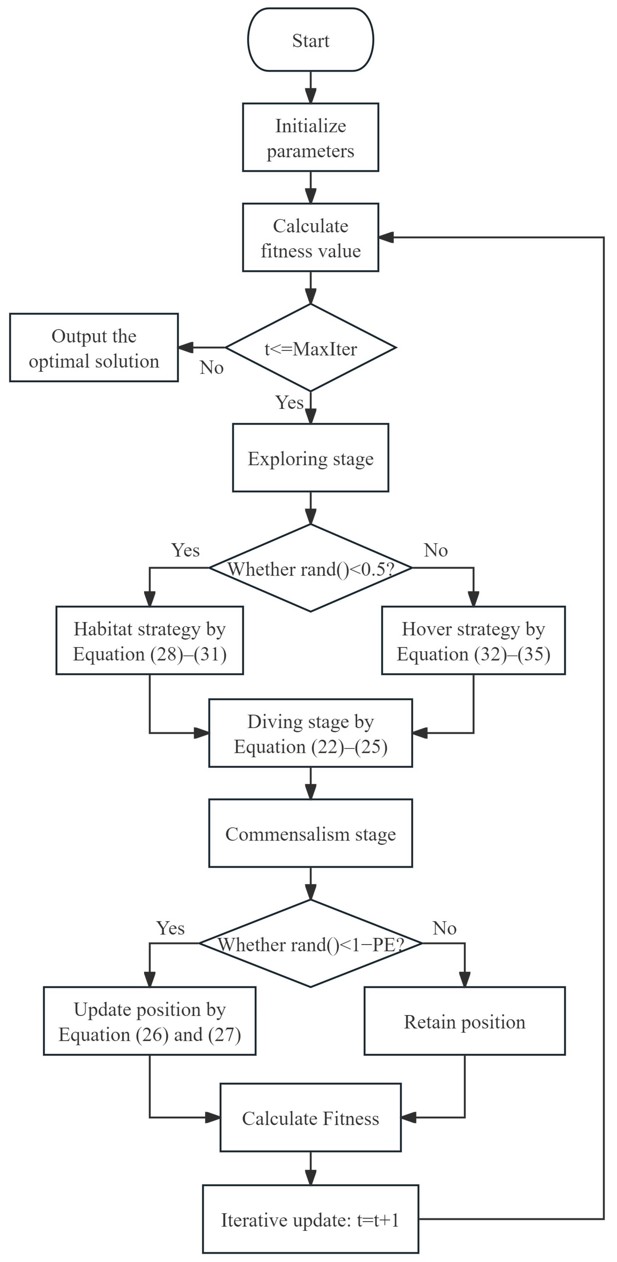
The original PKO suffers from low exploration of the solution space and poor local search capabilities. Inspired by the Marine Predator Algorithm (MPA) [36], this subsection proposes an improved PKO. This algorithm integrates the exploration phase of the PKO with the exploration phase of the MPA, which can effectively address the shortcomings of the original PKO and help the PKO escape from local optima. The exploration phase of the improved PKO algorithm is as follows.

When rand() < 0.5, the position is still updated using the original formula [36]:

$$X_i^{t+1}=X_i^t+\alpha \times T\times \left(X_j^t-X_i^t\right),$$

(28)

$$\alpha =2\times randn(1,D)-1,$$

(29)

$$T={beating}_{rate}\times {\left({\displaystyle \frac{t}{{Max}_{Iter}}}\right)}^{{\displaystyle \frac{1}{BF}}},$$

(30)

$${beating}_{rate}=rand\times \left({\displaystyle \frac{Fitness\left(j\right)}{Fitness\left(i\right)}}\right),$$

(31)

When 0.5 < rand() < 0.8, the position is updated using the exploration phase of the MPA. This stage simulates the high-speed movement of predators, employing Lévy flight to drive global search:

$$stepsize\left(i,j\right)=RL\left(i,j\right)\times \left(Elite\left(i,j\right)\hspace{0.25em}-Prey\left(i,j\right)\right),$$

(32)

$$Prey\left(i,j\right)=Prey\left(i,j\right)+P\times R\times stepsize\left(i,j\right),$$

(33)

where $\mathit{Prey}\left(i,j\right)$ is the $j$-th dimensional position of the $i$-th individual, $Elite\left(i,j\right)$ is the position of the optimal individual, $RL\left(i,j\right)$ is the Lévy flight random vector, $P = 0.5$ is the step size control parameter, and R is a random number in the interval [0, 1].

The relevant formulas for Lévy flight are as follows [36]:

$$RL=u/{\left|v\right|}^{{\displaystyle \frac{1}{\beta }}} ,$$

(34)

$${\sigma }_u={\left({\displaystyle \frac{\Gamma \left(1+\beta \right)\times sin\left(\frac{\Pi \beta }{2}\right)}{\Gamma \left(\frac{1+\beta }{2}\right)\times \beta \times \left(2^{\frac{\left(\beta -1\right)}{2}}\right)}}\right)}^{{\displaystyle \frac{1}{\beta }}},$$

(35)

where $\Gamma$ is the gamma function, $u$ and $v$ are used to calculate the magnitude and direction of the Lévy flight step size, $u ~ N(0, {\sigma }_u^2)$,$v ~ N(0, {\sigma }_v^2)$, ${\sigma }_v = 1$, and $\beta = 1.5$.

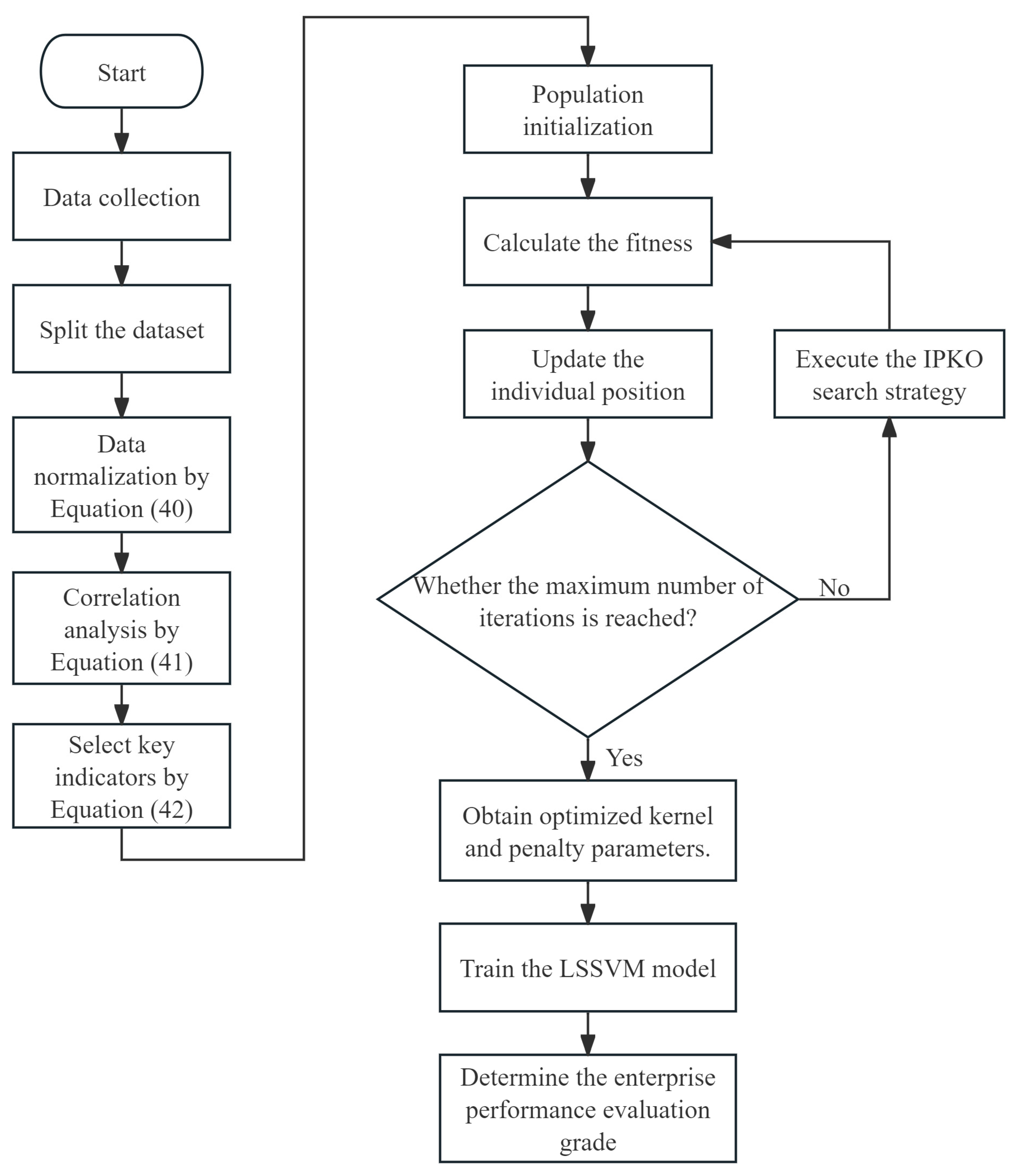
The flowchart of the IPKO is shown in Figure 1.

4.5. Model Framework and Its Evaluation Metric System

The performance evaluation method for building construction enterprises proposed in this paper is based on the LSSVM model, with hyperparameter tuning implemented using IPKO. This method includes steps such as data collection, performance level classification, data preprocessing, case analysis, and effectiveness evaluation. Figure 2 illustrates the flowchart of the performance evaluation method proposed in this paper.

The effectiveness evaluation of the IPKO-LSSVM model constitutes one of the pivotal research components in this study. To comprehensively assess its performance, three additional machine learning approaches, namely Backpropagation Neural Networks (BPNN), Random Forest (RF), and eXtreme Gradient Boosting (XGBoost), were employed for comparative analysis against the LSSVM model. All models were optimized by IPKO. The evaluation metrics employed for each model encompass Accuracy, Precision, Recall, and F1-Score, which are calculated as follows [58]:

$$\mathrm{A}\mathrm{c}\mathrm{c}\mathrm{u}\mathrm{r}\mathrm{a}\mathrm{c}\mathrm{y}={\displaystyle \frac{TP+TN}{TP+TN+FP+FN}},$$

(36)

$$\mathrm{P}\mathrm{r}\mathrm{e}\mathrm{c}\mathrm{i}\mathrm{s}\mathrm{i}\mathrm{o}\mathrm{n}={\displaystyle \frac{TP}{TP+FP}},$$

(37)

$$\mathrm{R}\mathrm{e}\mathrm{c}\mathrm{a}\mathrm{l}\mathrm{l}={\displaystyle \frac{TP}{TP+FN}},$$

(38)

$$\mathrm{F}1\text{-}\mathrm{S}\mathrm{c}\mathrm{o}\mathrm{r}\mathrm{e}=2\times {\displaystyle \frac{\mathrm{P}\mathrm{r}\mathrm{e}\mathrm{c}\mathrm{i}\mathrm{s}\mathrm{i}\mathrm{o}\mathrm{n}\times \mathrm{R}\mathrm{e}\mathrm{c}\mathrm{a}\mathrm{l}\mathrm{l}}{\mathrm{P}\mathrm{r}\mathrm{e}\mathrm{c}\mathrm{i}\mathrm{s}\mathrm{i}\mathrm{o}\mathrm{n}+\mathrm{R}\mathrm{e}\mathrm{c}\mathrm{a}\mathrm{l}\mathrm{l}}}.$$

(39)

where $TP$, $TN$, $FP$, and $FN$ represent the number of true positives, true negatives, false positives, and false negatives, respectively.

The modeling logic of the IPKO-LSSVM model constructed in this study strictly follows the theoretical framework of EBT. Specifically, the input layer of the model consists of environmental and behavioral variables from the EBT theoretical framework, and the output layer corresponds to the performance results in that framework. The training of the LSSVM model is essentially to fit the complex nonlinear mapping relationship of ‘environment–behavior-performance’ presented by sample data. The improved PKO algorithm determines the mapping relationship by searching for the optimal model parameters to obtain the most accurate mathematical expression. Therefore, this model is not a data-driven black box but an empirical model that translates EBT theory into a verifiable, computable framework.

5. Results

This section will conduct a case study using the performance evaluation model for building construction enterprises proposed earlier. The CPU of the computer used in the experiment is 12th Gen Intel (R) Core (TM) i7-12700H, the memory is 16 G, and the code was written in MATLAB 2022a.

5.1. Data Preprocessing

Based on the data acquisition method described above, the partial data obtained are shown in

Table 4. Partial sample data.

No.	${\mathit{E}}_1$	${\mathit{E}}_2$	${\mathit{E}}_3$	${\mathit{B}}_1$	${\mathit{B}}_2$	${\mathit{B}}_3$	${\mathit{B}}_4$	${\mathit{B}}_5$	${\mathit{B}}_6$	${\mathit{B}}_7$	${\mathit{B}}_8$	${\mathit{B}}_9$	${\mathit{B}}_{10}$	$\mathit{Y}$
(1)	5	6.3	5	3.05	71.70	1.75	1.58	96.5	4	5	5	2.15	0.08	V
(2)	5	5.2	5	0.85	86.6	1.08	2.39	95.9	5	5	4	3.55	0.09	IV
(3)	5	5.2	5	1.85	80.80	1.66	1.56	95.7	5	5	5	0.31	0.11	IV
(4)	5	6.0	5	0.65	91.64	0.93	1.61	96.8	5	5	5	0.81	0.07	III
(5)	5	5.2	5	2.63	88.13	0.96	0.59	96.2	5	5	5	1.85	0.1	IV
(6)	3	5.8	4	−7.10	94.91	0.94	0.82	84.6	4	5	4	1.88	0.14	II
$\dots$	$\dots$	$\dots$	$\dots$	$\dots$	$\dots$	$\dots$	$\dots$	$\dots$	$\dots$	$\dots$	$\dots$	$\dots$	$\dots$	$\dots$
(308)	2	8.4	1	0.13	83.8	1.18	1.08	86.8	3	2	1	1.21	0.41	I
(309)	2	8.9	2	0.97	84.2	1.17	1.11	87.6	3	2	3	0.93	0.36	II

, where $E_1-B_{10}$ correspond to the 13 secondary indicators selected in Table 1, and $Y$ represents the performance level. After preprocessing, this dataset can be used as input data to train and test the IPKO-LSSVM.

5.1.1. Division of Modeling Sample Set

A reasonable division of the data set helps improve the model’s generalization ability, avoid overfitting or underfitting, and ensure objective, accurate evaluation results. Considering that the number of samples collected is only 309, which belongs to the small sample problem, this paper randomly divides the training set and the test set according to the ratio of 7:3. In order to ensure the reproducibility of this article, the random number seed is set to 42.

Table 5. The basic situation of the training set and the test set.

Sample Set	Sample Size	Number of Samples for Each Performance Level
		I	II	III	IV	V
Training set	217	12	36	81	62	26
Test set	92	5	15	34	27	11

presents the basic situation of the divided training and test sets.

This paper uses 217 samples for the training set and 92 for the test set, with 81 and 34 samples at performance level III, respectively. The ratio between training and test sets is approximately 7:3, which also applies to the remaining performance levels.

5.1.2. Data Normalization

The machine learning model is sensitive to data quality and feature distribution, so it is necessary to normalize the original data to eliminate the influence of dimensional differences on model training. Min-Max Scaling was selected as the normalization method in this paper. This method preserves the relative magnitude of the data while stretching or compressing it to the target range.

For the j-th feature, let the original data be $x_{ij}$, and the normalized data be ${\overline{x}}_{ij}$. The following formula can be used to map all data to the range [0, 1]:

$${\overline{x}}_{ij}={\displaystyle \frac{x_{ij}-\mathrm{m}\mathrm{i}\mathrm{n}\left(x_{ij}\right)}{\mathrm{m}\mathrm{a}\mathrm{x}\left(x_{ij}\right)-\mathrm{m}\mathrm{i}\mathrm{n}\left(x_{ij}\right)}}$$

(40)

In this paper, Equation (40) is used to process the divided training set and test set, respectively, and then input them into the IPKO-LSSVM model for performance level evaluation.

5.2. Correlation Analysis

The Pearson correlation coefficient $\rho$ is used to measure the degree and direction of linear correlation between two continuous variables. When $\rho$ > 0.8, the correlation between the two variables is strong; when 0.7 < $\rho$ < 0.8, the correlation is moderate; and when $\rho$ < 0.7, the correlation is weak.

$$\rho ={\displaystyle \frac{\sum _{i=1}^n\left(x_i-\overline{x}\right)\left(y_i-\overline{y}\right)}{\sqrt{\sum _{i=1}^n{\left(x_i-\overline{x}\right)}^2{\left(y_i-\overline{y}\right)}^2}}}$$

(41)

where $x_i$ and $y_i$ represent the data values of two continuous variables, while $\overline{x}$ and $\overline{y}$ denote their respective means.

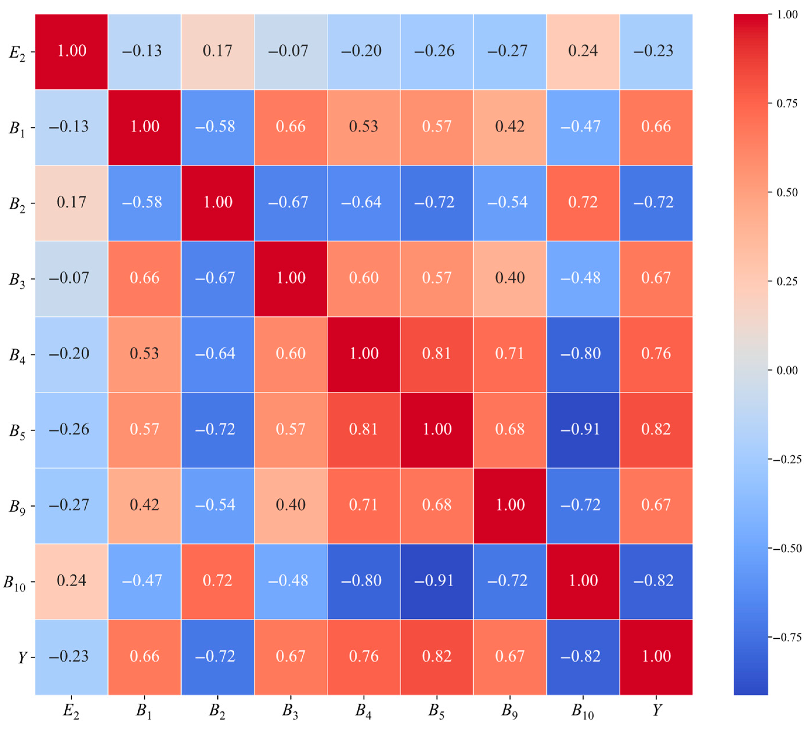
In this paper, the normalized data are substituted into Equation (41) to calculate the Pearson correlation coefficient. Figure 3 illustrates the correlations among continuous variables.

As shown in Figure 3, 75% of the indicators exhibit weak or moderate correlations with performance levels, suggesting that nonlinear methods, such as LSSVM, are suitable for performance evaluation in building construction enterprises.

5.3. Feature Selection

Feature selection plays an important role in the training of machine learning models, as it can effectively eliminate redundant features and improve model accuracy. This study employs the ReliefF algorithm for feature selection. The ReliefF algorithm, proposed by Kononenko [59], randomly selects a sample from the training set. For each sample $R_i$, it searches for $k$ nearest neighbors $H_j$ with the same class as $R_i$ and $k$ nearest neighbors $M_j$ with a different class from $R_i$. The weight of feature $A$ is then calculated according to the following formula [59]:

$$W(A)=W(A)-{\displaystyle \frac{1}{mk}}{\sum }_{j=1}^{k}diff(A,R_i,H_j)+{\displaystyle \frac{1}{mk}}{\sum }_{c\ne class\left(R_i\right)}\left[{\displaystyle \frac{p\left(c\right)}{1-p\left(class\right(R_i\left)\right)}}{\sum }_{j=1}^{k}diff(A,R_i,M_j(c\left)\right)\right],$$

(42)

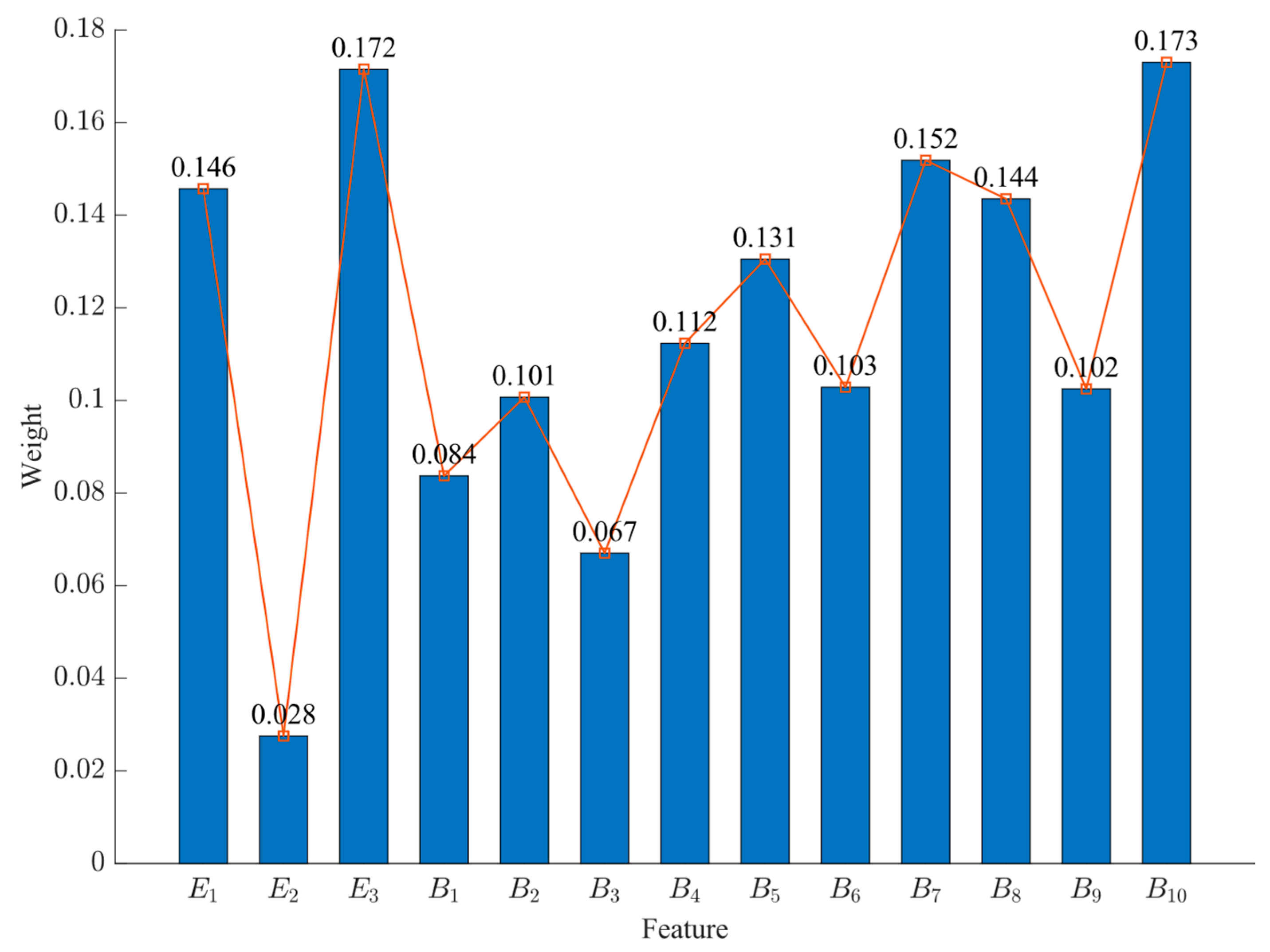
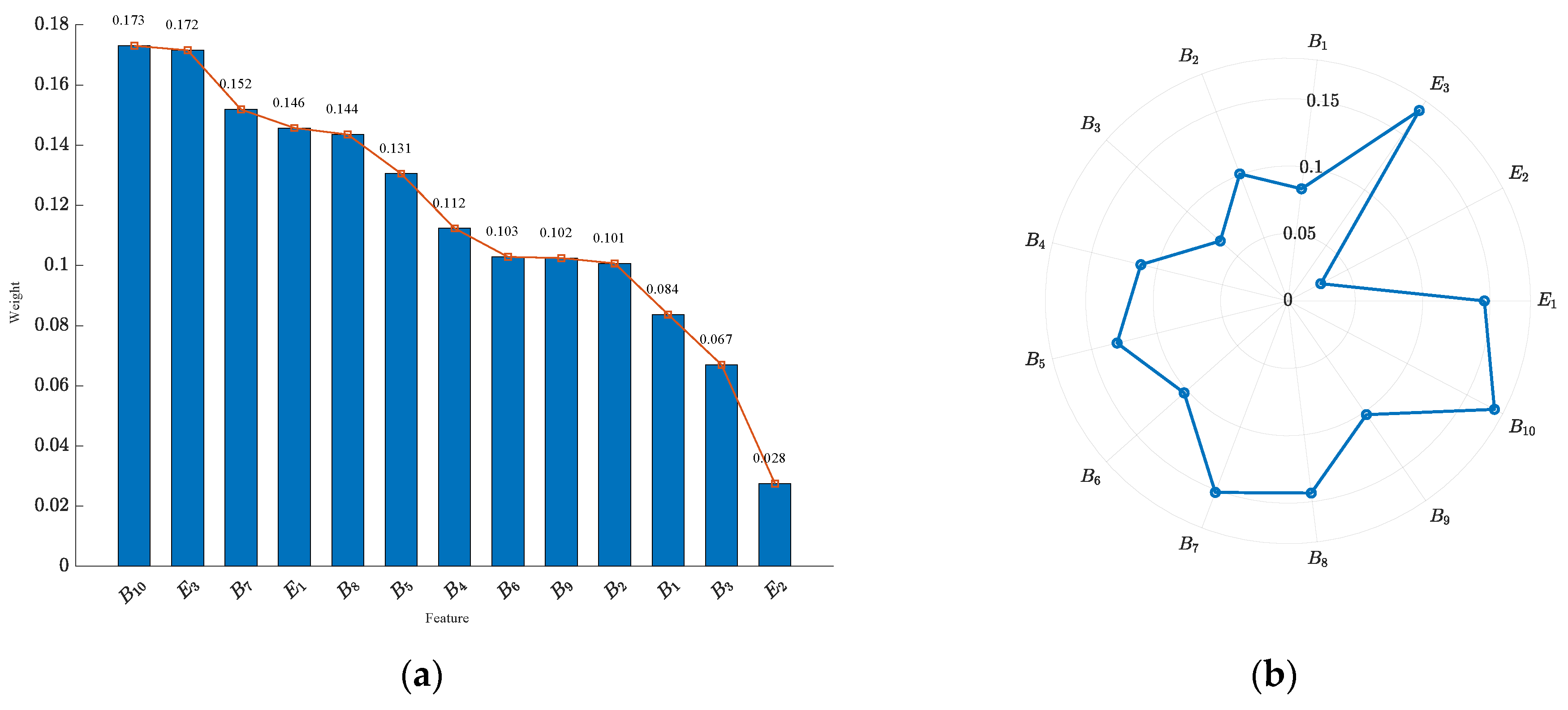
where $m$ is the number of iterations, $diff(\cdot )$ represents the distance, and $p(\cdot )$ denotes the prior probability of the target class. The ranking of weights for each indicator is shown in Figure 4.

It can be seen that the weight of the safety accident rate ($B_{10}$) is the highest, about 0.173. This is because the incidence of safety accidents is related to the operating qualifications and market reputation of building construction enterprises, and it is a red line for maintaining the sustainable development of building construction enterprises. The policy support ($E_3$) is the second-highest at 0.172. This is because policy support determines whether building construction enterprises are on a fast-growth track, which is a key factor in their sustainable development. The regional growth rate ($E_2$) has the lowest weight of 0.028. This may be because it takes a long time for changes in regional economic growth rates to affect the specific projects of building construction enterprises, which have little impact on enterprise performance in any given year. This study considers removing the two indicators with the lowest weights, namely $E_2$ and $B_3$. For a detailed discussion on how the model accuracy changes after removing different numbers of features, please refer to Section 6.

5.4. Cross-Validation and IPKO Parameter Optimization

Cross-validation is commonly used to evaluate the generalization ability of machine learning models on independent datasets. k-fold cross-validation is one of the most widely used techniques. Specifically, the dataset is randomly partitioned into $k$ mutually exclusive subsets of approximately equal size. In each of the $k$ iterations, $k-1$ subsets are combined to form the training set, while the remaining single subset serves as the validation set. This procedure is repeated $k$ times, ensuring that every subset serves as the validation set exactly once. The final model performance is reported as the average of the evaluation metrics obtained across all $k$ validation rounds.

In this paper, 5-fold cross-validation was used further to verify the generalization capability of the IPKO-LSSVM model and parameter optimization. The 217 samples in the training set were approximately evenly divided into five parts, and the fitness function for parameter optimization of the IPKO was set as the average misclassification rate of five experiments. In addition, the population size of IPKO is set to $N=10$, the maximum number of iterations is $T=100$, and the random walk parameter $\alpha =8$. The optimization range of parameter $\gamma$ for LSSVM is [1, 1000], and the optimization range of $\sigma$ is [0.1, 10].

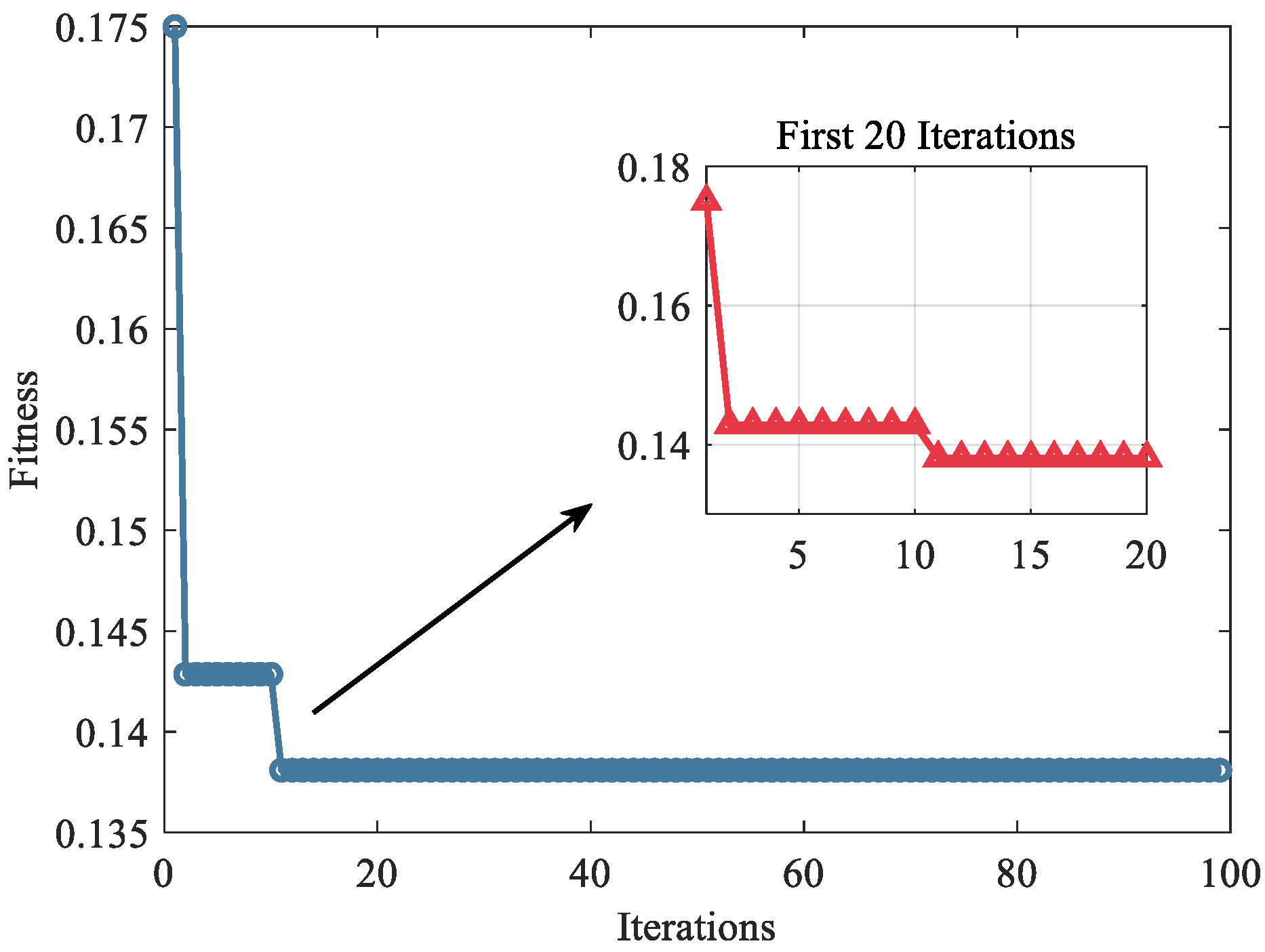
After inputting the validation set data and parameters, IPKO continuously searches for the optimal solution within the solution space range by virtue of its unique mechanism and finally converges to the optimal solution. Figure 5 shows the detailed process of IPKO parameter optimization.

In Figure 5, the fitness of IPKO decreased to approximately 0.143 within the first five generations. At the 11th generation, the fitness of IPKO decreased by 0.00476 compared to the 5th generation, which exceeded the threshold of 0.001, prompting IPKO to continue iterating. Subsequently, it eventually reached the maximum number of iterations, converging at 0.138. The optimal parameters for the LSSVM model were determined as $\gamma = 233.024$ and $\sigma = 3.084$.

Across the five experiments, the IPKO-LSSVM was evaluated on the validation sets and yielded accuracies of 83.33%, 88.10%, 88.10%, 88.10%, and 83.33%, precision values of 88.97%, 86.89%, 92.50%, 88.61%, and 87.87%, recall values of 86.47%, 87.14%, 82.65%, 92.16%, and 80.40%, and F1-scores of 0.8728, 0.8625, 0.8256, 0.8895, and 0.8225, respectively. Averaged across all five experiments, the model attained an accuracy of 86.19%, a precision of 88.97%, a recall of 85.76%, and an F1 score of 0.8546, indicating that the IPKO-LSSVM effectively captures underlying patterns in the data while maintaining a relatively low risk of overfitting.

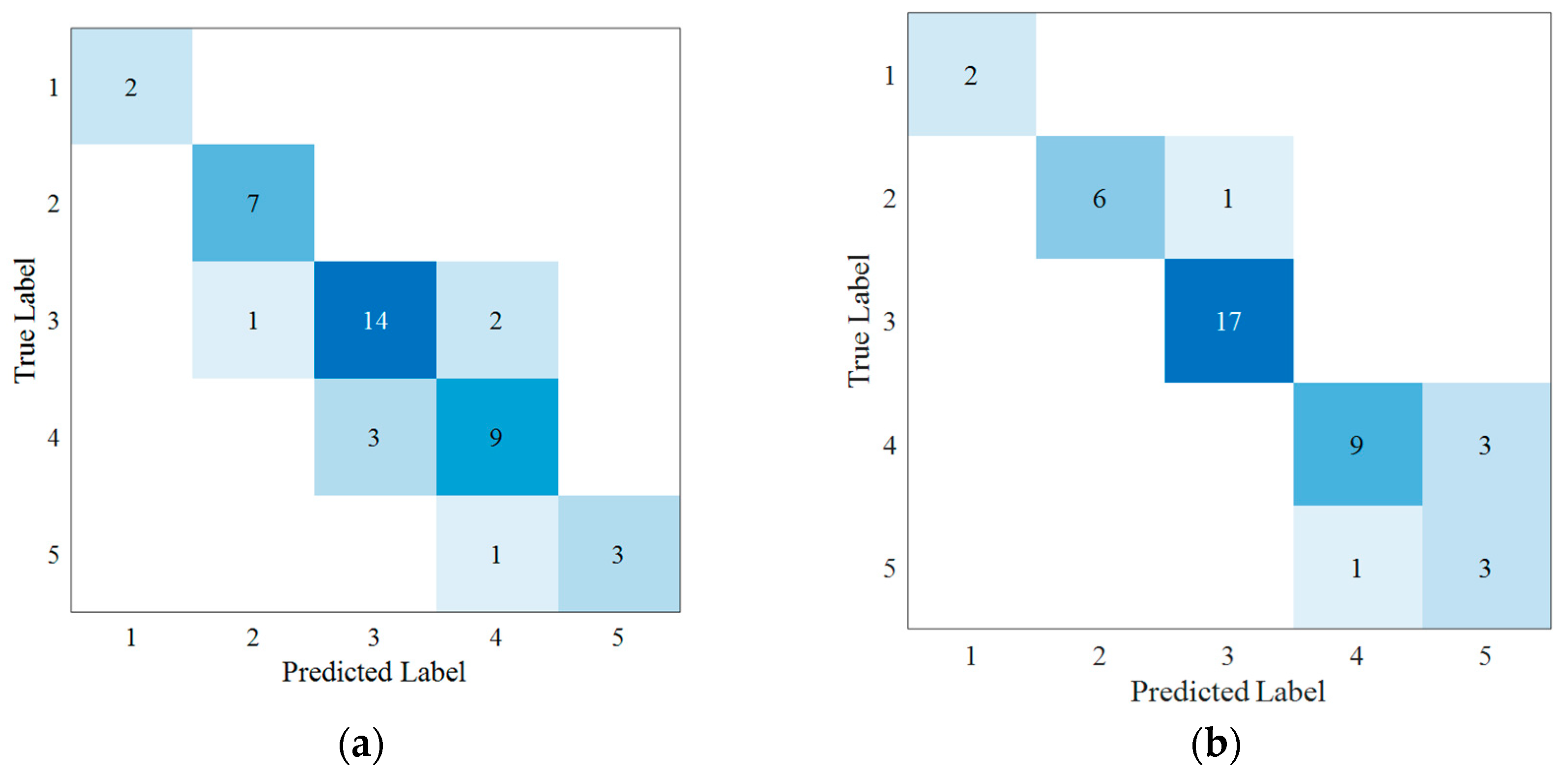
Furthermore, we plotted the confusion matrices obtained during the cross-validation process to provide a more intuitive illustration of the model’s classification performance on the validation set of each fold. As shown in Figure 6, the confusion matrices across the five experiments exhibit a consistently similar pattern: the number of correctly classified samples predominates in each category, while the number of misclassified samples remains relatively small, further confirming that the model maintains a low misclassification rate. These results collectively demonstrate that the IPKO-LSSVM possesses a certain degree of generalization capability and reliable classification performance on the current dataset.

5.5. Performance Evaluation of Building Construction Enterprises

In the previous subsection, we employed the IPKO to optimize hyperparameters for the LSSVM model. By constructing a two-dimensional search space and using average misclassification rate as the performance metric, we ultimately determined the optimal parameter combination. This subsection will substitute the optimal parameters into the LSSVM model for training.

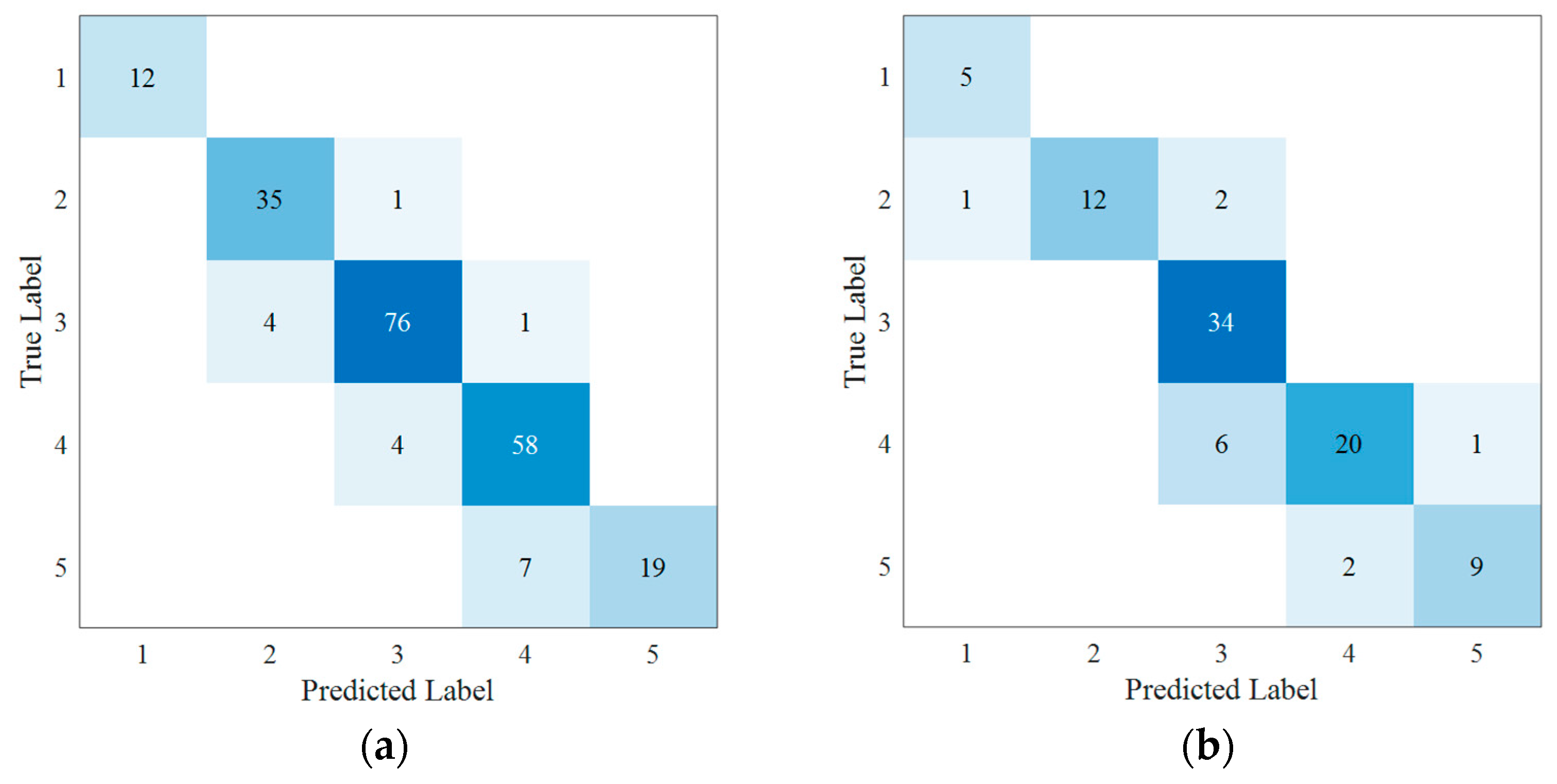
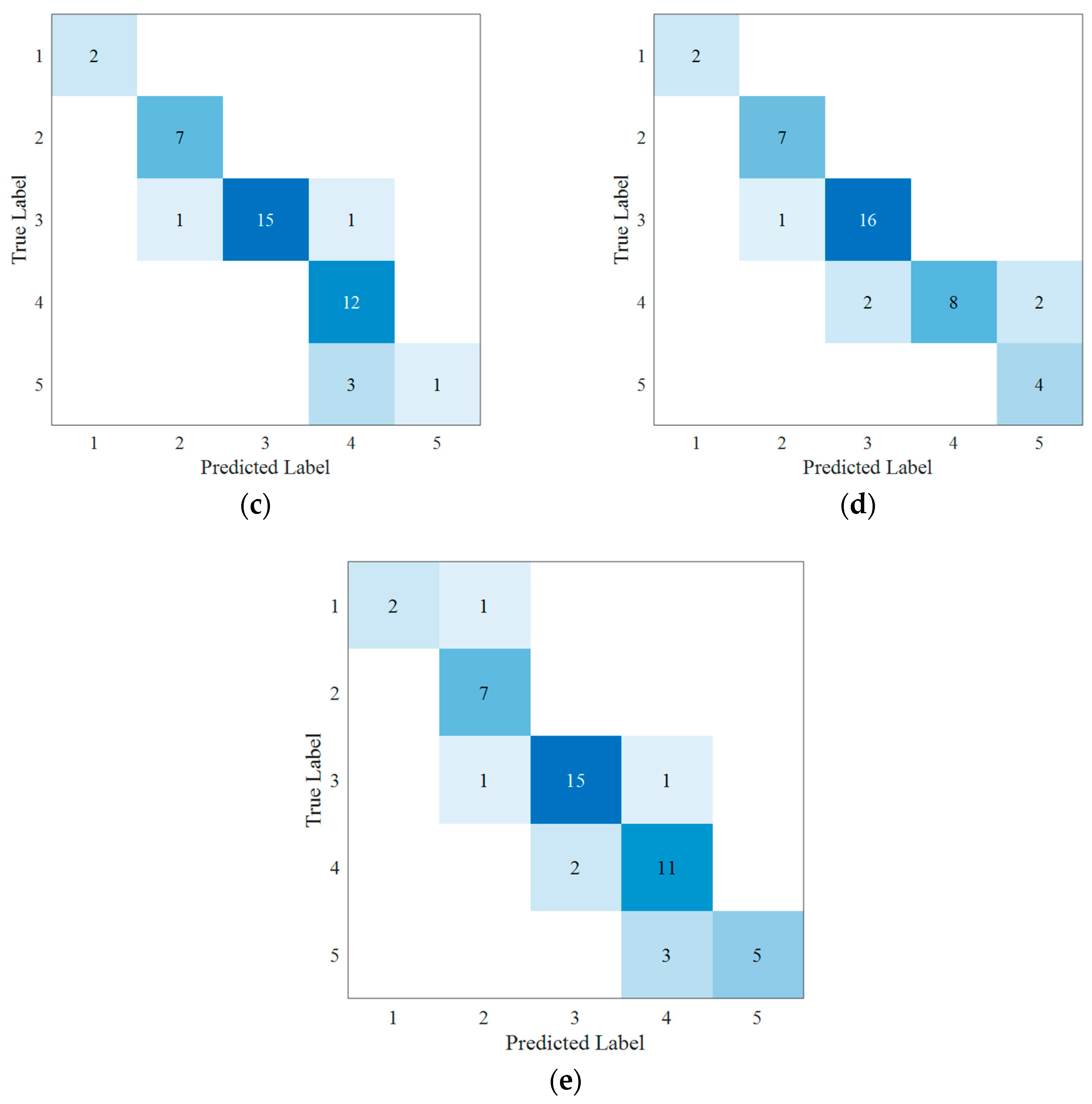
The IPKO-LSSVM model achieved an accuracy of 92.17%, a precision of 94.29%, a recall of 91.53%, and an F1-score of 0.9245 on the training set. In addition, the model achieved an accuracy of 86.96%, a precision of 89.04%, a recall of 87.18%, and an F1-score of 0.8732 on the test set. The confusion matrix composed of the results obtained from performance evaluation using this model is shown in Figure 7.

The confusion matrix clearly illustrates the model’s misclassification patterns, showing which categories it confuses. The training set misclassified 17 samples, while the test set misclassified 12. Among these misclassified samples, those with performance grades III and IV were incorrectly classified more frequently. This is because samples with performance grades III and IV exhibit high feature-space similarity, making it difficult for the model to learn a clear decision boundary. Specifically, employees in these two grades often demonstrate similar value distributions across multiple evaluation indicators, such as corporate social reputation and employee training levels.

In addition, we specifically selected the HNYJ group as a concrete case for analysis. By inputting the relevant data for this group into the established IPKO-LSSVM model, we obtained a performance evaluation result of III for the HNYJ group, indicating that its performance level is rated ‘Qualified’. This suggests that the building construction enterprise meets industry-average standards in key indicators and can meet standard operational requirements.

Financially, the enterprise shows average profitability with manageable financial risks but has weak risk resistance. In terms of market competitiveness, the enterprise has a presence but a limited market share, and its brand influence is relatively small. At the management level, basic systems and procedures are in place to support project management and quality control. However, efficiency and effectiveness need improvement. In terms of technological innovation, the enterprise primarily relies on traditional technical methods, adopts new technologies cautiously, and lacks independent research and development capabilities. In terms of social responsibility, the enterprise complies with basic laws and regulations but invests relatively little in environmental protection, public welfare, and employee benefits. HNYJ group can enhance its financial resilience by controlling costs and cash flow through refined management. At the same time, the group can accelerate the digitization and standardization of management processes to improve construction efficiency.

6. Discussion

6.1. The Performance of IPKO

This study selected PSO, WOA, SSA, DBO, OOA and PKO for comparison with the IPKO. The optimization performance of each algorithm was evaluated using the IEEE CEC2022 standard test set. The population size of the five algorithms mentioned above was set to $N=30$, the maximum number of iterations was $T=1000$, and the dimension of the test functions was $\dim =10$. Each algorithm was run 30 times on each benchmark function, and the average results were taken.

Table 6. The statistical indicators of the seven algorithms (dim = 10).

${\mathrm{F}}_1$	Best Value	Worst Value	Mean	Std	Median	Average Time	Rank
PSO	300.000	300.005	300.001	0.001	300.000	0.117	2
WOA	4049.864	45,493.167	19,712.323	8760.024	21,346.839	0.128	7
SSA	300.000	300.000	300.000	0.000	300.000	0.468	1
DBO	300.000	2238.815	572.760	594.935	305.517	0.314	5
OOA	3337.386	11,273.858	7943.181	2194.717	7975.032	0.313	6
PKO	300.003	324.033	301.950	4.517	300.573	0.391	4
IPKO	300.033	308.557	301.241	1.884	300.462	0.362	3
${\mathrm{F}}_2$	Best Value	Worst Value	Mean	Std	Median	Average Time	Rank
PSO	400.006	476.744	409.699	21.416	403.988	0.114	4
WOA	400.395	666.826	441.932	54.140	415.676	0.134	6
SSA	400.003	467.842	408.082	11.654	404.691	0.487	3
DBO	400.553	495.537	433.179	35.623	411.577	0.338	5
OOA	519.592	3002.611	1549.082	692.531	1448.938	0.330	7
PKO	400.005	408.916	406.796	2.601	406.911	0.413	2
IPKO	400.021	408.916	406.377	3.032	407.047	0.394	1
${\mathrm{F}}_3$	Best Value	Worst Value	Mean	Std	Median	Average Time	Rank
PSO	600.001	630.642	610.580	9.039	608.442	0.212	4
WOA	614.238	656.266	637.330	10.899	638.215	0.234	6
SSA	600.000	631.282	604.712	6.711	601.692	0.681	3
DBO	600.799	628.529	612.175	8.795	609.913	0.465	5
OOA	625.279	669.013	645.433	10.219	645.100	0.515	7
PKO	600.000	600.007	600.001	0.002	600.000	0.617	2
IPKO	600.000	600.001	600.000	0.000	600.000	0.595	1
${\mathrm{F}}_4$	Best Value	Worst Value	Mean	Std	Median	Average Time	Rank
PSO	802.985	847.758	820.297	9.262	818.904	0.131	3
WOA	815.207	892.168	840.231	16.651	839.726	0.159	6
SSA	814.924	848.753	829.851	7.028	829.849	0.512	4
DBO	812.333	860.692	832.418	11.635	829.438	0.371	5
OOA	825.769	866.290	851.176	10.589	855.404	0.366	7
PKO	805.970	836.813	816.317	6.916	815.919	0.458	2
IPKO	803.980	825.869	813.366	5.276	811.442	0.447	1
${\mathrm{F}}_5$	Best Value	Worst Value	Mean	Std	Median	Average Time	Rank
PSO	900.000	1446.539	934.500	114.839	900.000	0.169	4
WOA	958.715	1985.978	1367.011	277.986	1361.327	0.204	7
SSA	920.364	1482.315	1353.998	205.273	1467.952	0.643	5
DBO	904.519	1257.867	981.127	100.209	928.346	0.454	3
OOA	1141.279	1752.513	1357.116	151.000	1317.992	0.470	6
PKO	900.000	900.000	900.000	0.000	900.000	0.575	2
IPKO	900.000	900.000	900.000	0.000	900.000	0.536	1
${\mathrm{F}}_6$	Best Value	Worst Value	Mean	Std	Median	Average Time	Rank
PSO	1821.118	13,998.092	3846.378	2637.621	2687.876	0.108	1
WOA	2044.185	8156.548	4120.482	1867.118	3543.258	0.134	3
SSA	1818.841	8127.246	4635.014	1994.475	4363.223	0.478	4
DBO	1954.870	8232.359	4646.832	2227.344	4372.185	0.333	5
OOA	2129.761	30,934,006.602	5,199,714.290	9,175,983.028	669,935.090	0.313	7
PKO	1848.617	8114.343	4965.168	2296.427	5098.202	0.407	6
IPKO	1830.582	8014.258	3916.230	1955.216	3609.334	0.391	2
${\mathrm{F}}_7$	Best Value	Worst Value	Mean	Std	Median	Average Time	Rank
PSO	2000.996	2072.143	2032.406	15.819	2029.946	0.257	4
WOA	2025.312	2129.490	2069.285	31.684	2056.990	0.276	6
SSA	2000.995	2068.615	2027.319	13.513	2021.984	0.767	3
DBO	2021.619	2070.806	2033.719	12.432	2029.791	0.532	5
OOA	2046.404	2147.025	2087.619	26.288	2084.644	0.612	7
PKO	2000.001	2030.574	2017.517	8.711	2021.055	0.760	2
IPKO	2000.001	2022.537	2016.630	8.411	2020.995	0.740	1
${\mathrm{F}}_8$	Best Value	Worst Value	Mean	Std	Median	Average Time	Rank
PSO	2202.112	2344.138	2236.048	42.174	2220.442	0.292	7
WOA	2219.070	2274.299	2232.627	9.747	2230.106	0.310	6
SSA	2201.431	2342.602	2225.090	22.595	2221.085	0.777	3
DBO	2221.235	2241.041	2228.070	5.094	2227.844	0.531	4
OOA	2223.943	2253.634	2232.536	6.808	2230.835	0.675	5
PKO	2202.375	2223.888	2220.102	4.919	2220.974	0.787	2
IPKO	2200.864	2222.882	2220.074	3.691	2220.515	0.762	1
${\mathrm{F}}_9$	Best Value	Worst Value	Mean	Std	Median	Average Time	Rank
PSO	2485.502	2676.216	2491.859	34.820	2485.502	0.213	1
WOA	2529.784	2712.019	2598.353	52.048	2601.021	0.231	6
SSA	2529.284	2529.840	2529.321	0.141	2529.284	0.656	4
DBO	2529.284	2636.722	2542.721	24.949	2533.330	0.470	5
OOA	2672.946	2829.580	2750.265	35.364	2748.305	0.548	7
PKO	2529.284	2529.284	2529.284	0.000	2529.284	0.595	2
IPKO	2529.284	2529.284	2529.284	0.000	2529.284	0.589	2
${\mathrm{F}}_{10}$	Best Value	Worst Value	Mean	Std	Median	Average Time	Rank
PSO	2500.174	3302.514	2596.150	148.948	2614.893	0.191	7
WOA	2500.644	3329.934	2686.938	269.591	2626.862	0.216	5
SSA	2403.602	3003.215	2638.455	128.053	2631.664	0.610	4
DBO	2500.462	2654.875	2525.111	54.913	2501.027	0.417	3
OOA	2520.109	2957.972	2691.919	108.110	2683.012	0.471	6
PKO	2500.282	2500.597	2500.403	0.088	2500.412	0.561	2
IPKO	2500.129	2500.525	2500.361	0.085	2500.366	0.559	1
${\mathrm{F}}_{11}$	Best Value	Worst Value	Mean	Std	Median	Average Time	Rank
PSO	2750.476	4475.102	2993.997	328.697	2900.001	0.262	6
WOA	2619.584	3060.751	2936.160	78.741	2941.603	0.295	5
SSA	2600.000	2912.721	2845.927	100.727	2900.000	0.724	4
DBO	2600.000	3213.030	2792.925	144.617	2750.497	0.469	3
OOA	2911.379	4627.606	3966.462	493.553	4054.879	0.622	7
PKO	2600.000	2900.000	2770.000	151.202	2900.000	0.714	2
IPKO	2600.000	2900.000	2660.000	122.051	2600.000	0.691	1
${\mathrm{F}}_{12}$	Best Value	Worst Value	Mean	Std	Median	Average Time	Rank
PSO	2848.532	2966.377	2875.872	32.198	2857.394	0.275	5
WOA	2864.791	3034.011	2894.295	38.224	2875.012	0.302	6
SSA	2861.435	2910.090	2867.261	8.517	2865.174	0.787	3
DBO	2863.269	2936.004	2873.870	15.160	2868.292	0.518	4
OOA	2900.724	3300.246	3061.735	81.360	3048.233	0.655	7
PKO	2859.369	2863.495	2861.920	1.024	2861.435	0.741	1
IPKO	2858.620	2863.495	2861.953	0.959	2861.435	0.728	2

presents the statistical indicators for different algorithms across test functions, including the mean, standard deviation, best and worst values, median, and average fitness running time over 30 experiments. The best–performing algorithm and its corresponding data for each benchmark function are highlighted in bold.

As shown in Table 6, the IPKO demonstrates the best optimization performance. The average rankings of the seven algorithms are 4.00, 5.75, 3.42, 4.33, 6.58, 2.42 and 1.42, respectively. Therefore, the performance ranking of each algorithm is IPKO > PKO > SSA > PSO > DBO> WOA > OOA. The average optimal fitness values of the IPKO on most benchmark functions are closer to the theoretical values than those of PKO. On benchmark function F6, the average optimal fitness of the PKO is 4965.168, while that of the IPKO is 3916.230, which is approximately 21.12% lower than that of the PKO. On benchmark function F11, the average optimal fitness of the PKO is 2770.000, while that of the IPKO is 2660.000, which is approximately 3.97% lower than that of the PKO. In addition, the IPKO achieves first place on eight benchmark functions.

Although its optimization performance is slightly inferior to other algorithms on some functions, the average optimal fitness remains close to the theoretical values. Compared with PKO and SSA, IPKO has lower computational time, with reductions of approximately 10% and 15% across multiple benchmark functions. However, the calculation time of IPKO is higher than that of the PSO, WOA, DBO, and OOA, which still presents certain limitations.

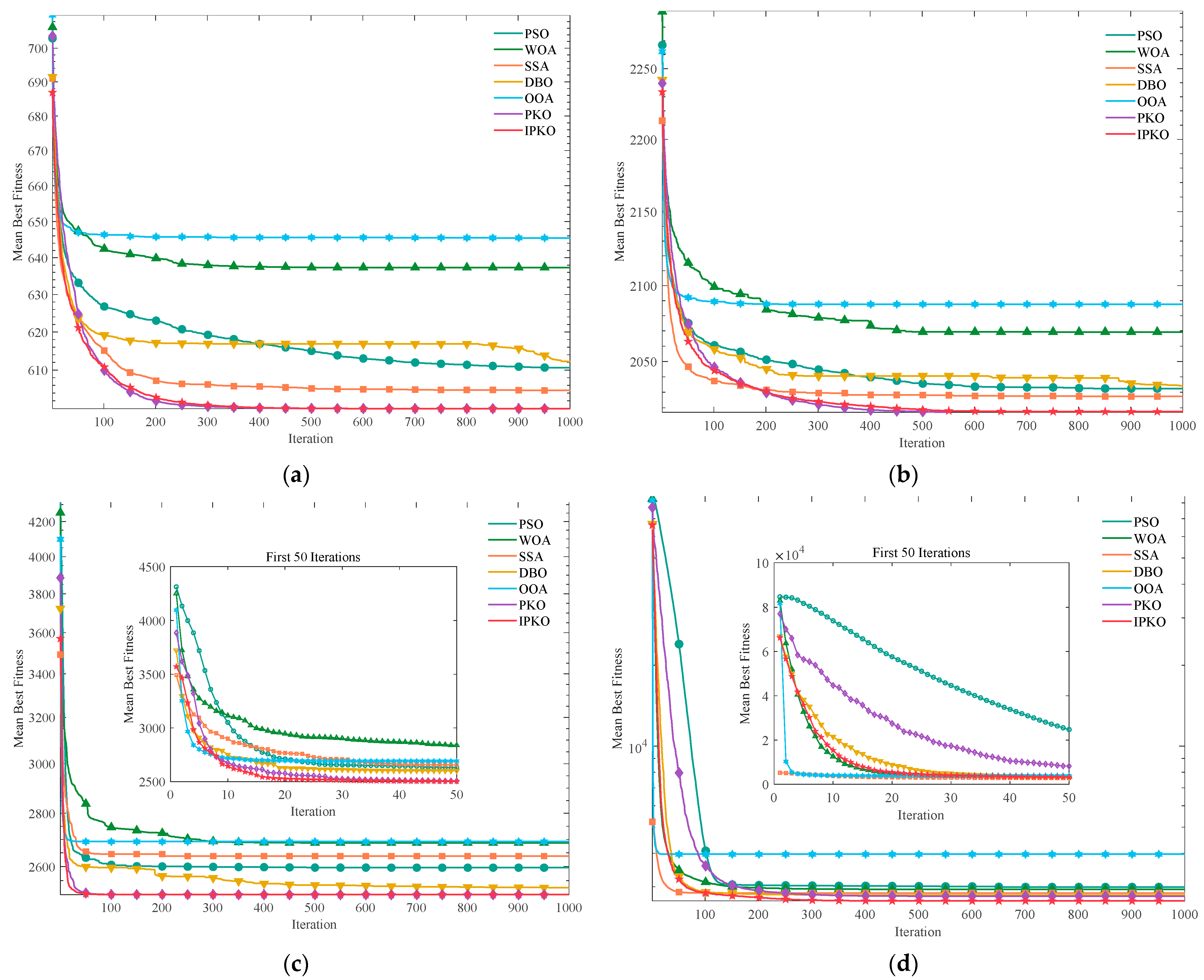
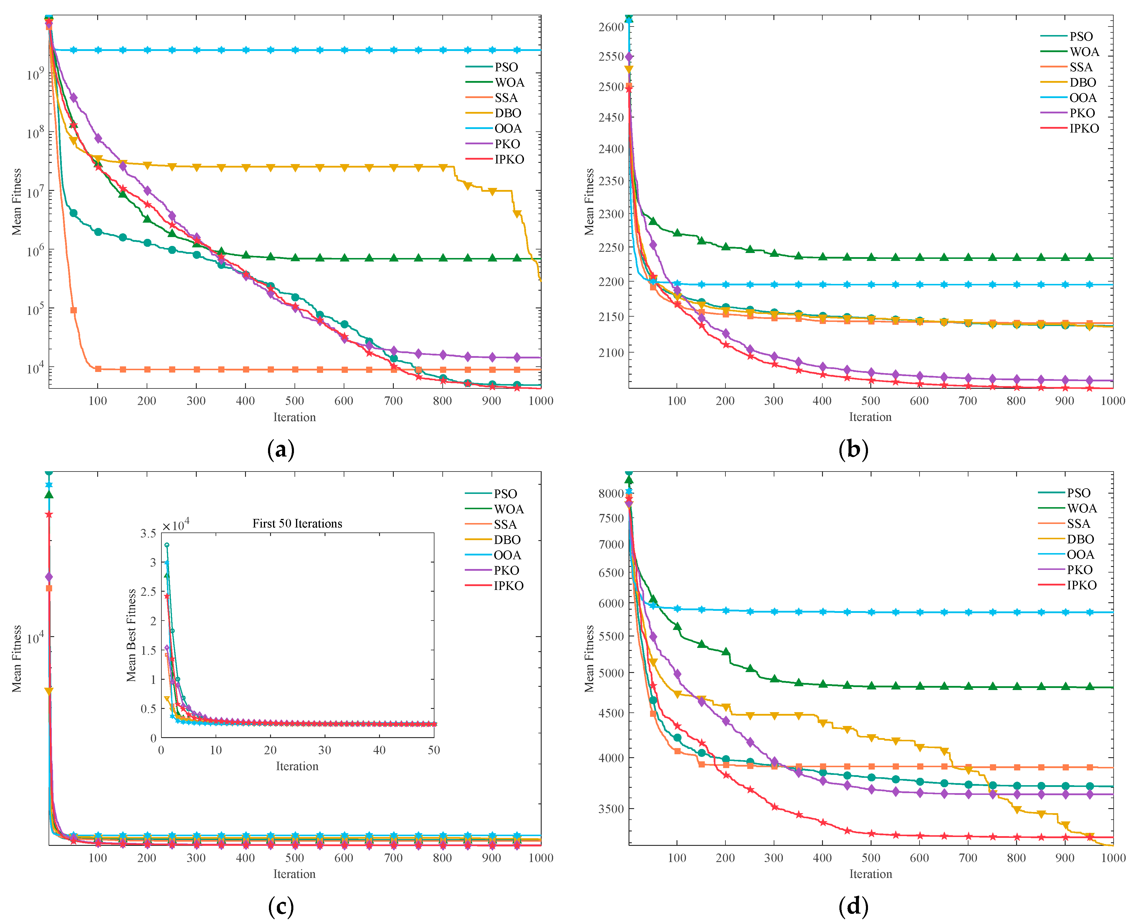
In addition, we have plotted the mean fitness curves for each algorithm. Due to space limitations, we only present a subset of the figures. Figure 8 demonstrates that IPKO exhibits strong performance across multiple complex problems and successfully escapes local optima on several occasions.

To further evaluate the performance of the IPKO, this paper keeps other parameters unchanged and only changes the dimension of the benchmark functions to dim = 20. On this basis, comparative experiments were conducted, and the experimental results are shown in

Table 7. The statistical indicators of the seven algorithms (dim = 20).

${\mathrm{F}}_1$	Best Value	Worst Value	Mean	Std	Median	Average Time	Rank
PSO	310.725	339.322	319.205	7.004	318.157	0.149	2
WOA	13,485.544	33,942.814	23,216.775	5564.383	22,617.944	0.151	5
SSA	303.894	2470.346	817.311	628.325	536.938	0.507	1
DBO	10,515.967	45,402.783	26,547.635	8975.896	23,755.031	0.367	6
OOA	29,881.318	107,886.771	49,108.997	15,726.453	44,802.261	0.330	7
PKO	4872.420	26,228.599	12,762.191	5217.986	11,003.246	0.439	4
IPKO	4181.956	16,844.570	8379.659	2729.741	7985.423	0.427	3
${\mathrm{F}}_2$	Best Value	Worst Value	Mean	Std	Median	Average Time	Rank
PSO	407.913	475.783	433.651	26.118	418.586	0.143	1
WOA	472.095	694.870	565.937	69.448	558.745	0.147	6
SSA	400.834	475.434	447.969	19.216	449.084	0.494	2
DBO	412.954	673.600	494.807	65.683	475.874	0.334	5
OOA	1744.538	5177.540	3133.800	883.504	3100.313	0.326	7
PKO	449.096	474.890	451.953	7.638	449.129	0.436	3
IPKO	445.005	474.839	455.528	10.913	449.237	0.424	4
${\mathrm{F}}_3$	Best Value	Worst Value	Mean	Std	Median	Average Time	Rank
PSO	617.456	658.836	638.662	9.330	638.572	0.317	5
WOA	649.894	711.385	668.133	13.056	668.268	0.320	6
SSA	608.379	655.765	631.511	11.023	631.186	0.776	3
DBO	608.133	658.595	632.140	12.104	632.663	0.522	4
OOA	647.789	695.805	677.240	10.227	677.378	0.672	7
PKO	600.000	600.858	600.192	0.215	600.147	0.799	2
IPKO	600.051	600.553	600.153	0.099	600.115	0.795	1
${\mathrm{F}}_4$	Best Value	Worst Value	Mean	Std	Median	Average Time	Rank
PSO	839.800	918.410	867.029	19.005	864.675	0.184	3
WOA	883.695	988.983	921.191	31.052	909.858	0.189	6
SSA	864.672	928.349	892.841	13.226	889.546	0.557	4
DBO	846.879	975.651	911.783	27.180	908.391	0.382	5
OOA	930.440	1000.012	969.479	16.183	974.032	0.406	7
PKO	829.226	874.622	849.429	13.548	851.738	0.506	2
IPKO	823.879	875.527	847.654	15.139	848.751	0.504	1
${\mathrm{F}}_5$	Best Value	Worst Value	Mean	Std	Median	Average Time	Rank
PSO	1099.400	3033.297	2105.968	496.664	2163.400	0.197	4
WOA	1819.983	6688.204	3564.762	1148.225	3130.215	0.206	7
SSA	1566.789	2738.603	2329.334	292.421	2423.405	0.593	5
DBO	1061.290	3960.880	1993.528	650.892	1882.195	0.392	3
OOA	2381.775	5019.173	3511.010	607.411	3452.793	0.428	6
PKO	900.035	1735.409	994.246	169.621	926.896	0.536	2
IPKO	900.000	1017.175	908.621	22.031	901.662	0.525	1
${\mathrm{F}}_6$	Best Value	Worst Value	Mean	Std	Median	Average Time	Rank
PSO	1907.670	29,703.801	4863.769	5738.770	2564.476	0.145	2
WOA	41,098.301	4,596,420.875	688,866.470	916,653.150	393,823.270	0.155	6
SSA	1865.691	25,010.580	8928.162	8346.611	5077.590	0.519	3
DBO	2452.731	3,039,116.595	280,377.346	653,190.853	18,473.925	0.342	5
OOA	1.065 × 109	5.660 × 109	2.449 × 109	1.180 × 109	2.127 × 109	0.313	7
PKO	1897.637	25,596.720	14,310.629	9955.676	15925.591	0.436	4
IPKO	2192.440	15,020.083	4249.666	2407.188	3972.449	0.427	1
${\mathrm{F}}_7$	Best Value	Worst Value	Mean	Std	Median	Average Time	Rank
PSO	2057.633	2279.556	2136.473	54.441	2125.486	0.376	4
WOA	2122.415	2464.643	2233.734	79.163	2223.061	0.388	7
SSA	2046.206	2414.607	2140.655	84.430	2116.780	0.916	5
DBO	2078.797	2233.956	2135.479	44.186	2113.815	0.586	3
OOA	2143.847	2275.732	2195.376	29.683	2190.430	0.782	6
PKO	2024.750	2125.553	2061.464	26.993	2061.338	0.903	2
IPKO	2022.432	2114.835	2050.965	21.155	2049.332	0.900	1
${\mathrm{F}}_8$	Best Value	Worst Value	Mean	Std	Median	Average Time	Rank
PSO	2222.308	2797.285	2313.005	140.249	2228.493	0.465	5
WOA	2234.409	2523.866	2302.575	80.512	2258.701	0.464	4
SSA	2221.535	2460.396	2297.434	75.821	2253.240	1.042	3
DBO	2223.285	2502.670	2324.298	87.716	2318.347	0.687	6
OOA	2236.415	2724.518	2390.259	156.629	2350.162	0.947	7
PKO	2221.233	2254.637	2226.277	6.700	2224.170	1.067	2
IPKO	2220.687	2228.507	2223.039	1.666	2222.748	1.040	1
${\mathrm{F}}_9$	Best Value	Worst Value	Mean	Std	Median	Average Time	Rank
PSO	2465.346	2465.374	2465.359	0.008	2465.357	0.387	1
WOA	2504.988	2645.397	2554.253	40.548	2536.767	0.384	6
SSA	2480.781	2480.804	2480.785	0.008	2480.781	0.917	2
DBO	2480.804	2609.901	2506.456	31.797	2496.975	0.606	5
OOA	2830.885	5012.130	3454.637	529.701	3308.914	0.801	7
PKO	2480.782	2480.909	2480.809	0.030	2480.797	0.902	4
IPKO	2480.781	2481.207	2480.798	0.077	2480.783	0809	3
${\mathrm{F}}_{10}$	Best Value	Worst Value	Mean	Std	Median	Average Time	Rank
PSO	2500.397	4995.410	3711.292	909.093	3940.615	0.299	4
WOA	2501.195	6273.223	4811.128	1218.311	5147.982	0.306	6
SSA	2500.879	4959.062	3897.766	791.276	4098.703	0.789	5
DBO	2500.934	5847.136	3177.323	1116.381	2501.901	0.520	1
OOA	2610.276	7401.351	5852.332	1580.832	6361.502	0.647	7
PKO	2500.440	4988.423	3634.044	870.305	3953.895	0.748	3
IPKO	2500.517	5221.770	3246.204	902.197	2500.801	0.724	2
${\mathrm{F}}_{11}$	Best Value	Worst Value	Mean	Std	Median	Average Time	Rank
PSO	2900.669	5883.114	3001.193	544.308	2901.770	0.470	5
WOA	3104.659	4324.252	3470.549	227.744	3433.006	0.476	6
SSA	2600.000	3000.000	2926.667	78.492	2900.000	1.072	4
DBO	2600.000	3086.753	2910.085	75.479	2900.000	0.679	3
OOA	8166.170	10,165.982	9143.636	493.016	9193.944	0.976	7
PKO	2900.260	2900.845	2900.476	0.147	2900.434	1.094	2
IPKO	2900.000	2900.569	2900.198	0.195	2900.205	1.091	1
${\mathrm{F}}_{12}$	Best Value	Worst Value	Mean	Std	Median	Average Time	Rank
PSO	2890.984	3690.732	3153.619	257.145	3176.139	0.501	6
WOA	2954.932	3384.008	3074.052	113.156	3033.928	0.513	5
SSA	2944.850	3082.631	2998.506	37.496	2991.864	1.158	3
DBO	2950.947	3299.830	3057.088	79.570	3043.533	0.733	4
OOA	3550.864	4471.066	4100.108	237.469	4157.030	1.047	7
PKO	2936.830	2985.598	2943.716	8.408	2941.734	1.156	1
IPKO	2936.831	2969.902	2943.946	5.808	2942.116	1.152	2

. The best–performing algorithm and its corresponding data for each benchmark function are highlighted in bold.

Based on Table 7, the average rankings of the seven algorithms on the CEC2022 standard test set with dim = 20 are 3.50, 5.83, 3.33, 4.167, 6.833, 2.53, and 1.75, respectively. Therefore, the performance ranking of each algorithm is IPKO > PKO > SSA > PSO > DBO > WOA > OOA. IPKO demonstrates superior global optimization capability. The partial mean fitness curves of each algorithm on the benchmark functions when dim = 20 are shown in Figure 9.

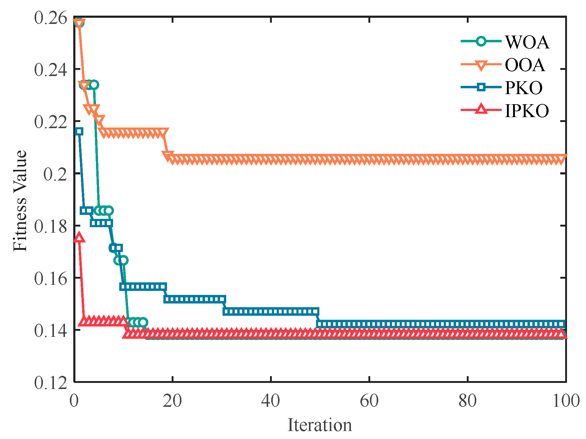
The performance of the IPKO in the LSSVM parameter optimization problem is also worth discussing. This paper selects WOA, OOA and PKO, for LSSVM parameter optimization and compares their parameter optimization processes with IPKO. Figure 10 shows the fitness curves of each algorithm.

In Figure 10, the IPKO converges the fastest, with its fitness rapidly decreasing to approximately 0.142 within the first few generations, then dropping further to around 0.138 near the 15th generation and finally converging. The WOA’s fitness decreases to approximately 0.18 in the early generations, subsequently escaping local optima multiple times. The PKO demonstrates moderate parameter optimization capability, eventually converging at approximately 0.138, while the OOA exhibits the poorest optimization ability, converging only at approximately 0.206.

6.2. The Performance of LSSVM

The model’s predictive outcomes are partially influenced by dataset partitioning, making appropriate partitioning strategies crucial for improving accuracy. This study employed multiple partitioning approaches, applying training and test sets in ratios of 6:4, 7:3, 8:2, and 9:1 to the IPKO-LSSVM model to evaluate their impact on prediction performance. The model’s performance metrics under different partitioning ratios are presented in

Table 8. The influence of different proportions of the training set and the test set on performance evaluation results.

Training set	Proportion	Accuracy	Precision	Recall	F1-Score
	90%	91.01%	91.32%	90.99%	0.9100
	80%	91.53%	92.97%	92.34%	0.9258
	70%	92.17%	94.29%	91.53%	0.9245
	60%	92.43%	94.11%	92.58%	0.9324
Test set	Proportion	Accuracy	Precision	Recall	F1-Score
	10%	84.02%	82.36%	80.13%	0.8093
	20%	85.25%	88.37%	79.17%	0.8274
	30%	86.96%	89.04%	87.18%	0.8732
	40%	83.87%	85.03%	82.38%	0.8342

.

As the test set proportion increased from 10% to 30%, the accuracy and recall improved. However, when the proportion further rose to 40%, the model’s performance metrics declined. This indicates that the optimal training performance is achieved when the proportion of the training set and test set is 7:3. Therefore, this study adopts a 7:3 split for the data set.

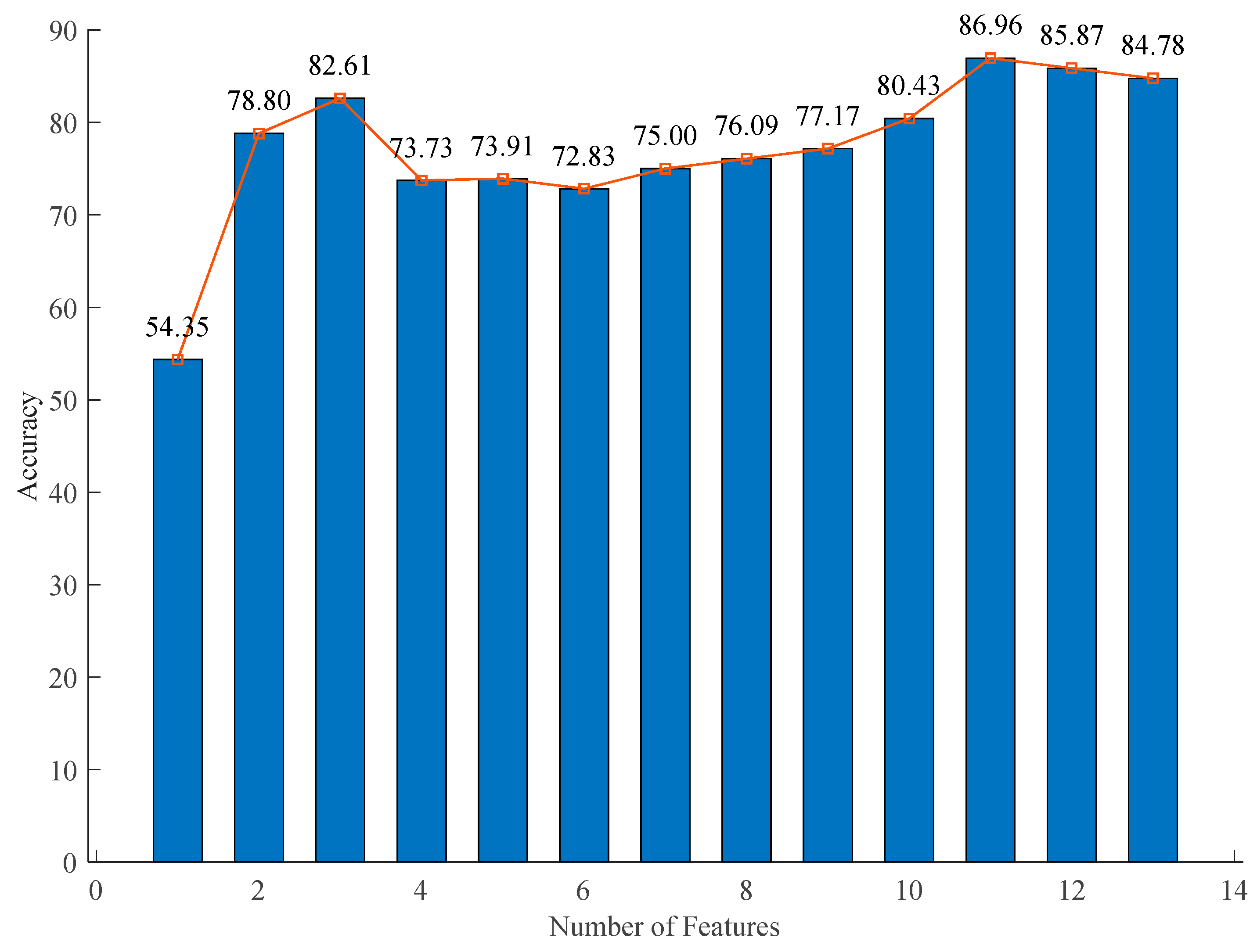
Feature selection improves the model’s accuracy. The following discussion will focus on improving the IPKO-LSSVM model’s performance using the ReliefF algorithm. Figure 11 shows the test set accuracy of the IPKO-LSSVM model as the number of features varies.

The results in Figure 11 show that when selecting 11 features, the IPKO-LSSVM model achieves the highest testset accuracy, improving by 2.18% compared to using all features.

To further demonstrate the superiority of the IPKO-LSSVM model, this paper compares it with BPNN, RF, and XGBoost, all of which use IPKO for parameter optimization. The performance of each model on the test set is shown in

Table 9. The performance of different machine learning models.

Model	Accuracy	Precision	Recall	F1-Score
IPKO-BPNN	80.43%	83.24%	77.09%	0.7874
IPKO-RF	82.80%	84.71%	78.70%	0.8093
IPKO-XGBoost	80.22%	75.37%	72.05%	0.7213
IPKO-LSSVM	86.96%	89.04%	87.18%	0.8732

.

From the experimental results in Table 9, it can be seen that the IPKO-LSSVM model significantly outperforms the other three comparison models in all evaluation metrics, fully demonstrating the superiority of the IPKO-LSSVM method. Specifically, the accuracy of IPKO-LSSVM reaches 90.22%, which is an improvement of 6.53%, 4.16%, and 6.74% over IPKO-BPNN, IPKO-RF, and IPKO-XGBoost, respectively.

In terms of precision, IPKO-LSSVM performs excellently, achieving 89.04%, nearly 14% higher than IPKO-XGBoost (75.37%), indicating that this model is more reliable at identifying positive samples and has a lower false-positive rate. For the recall metric, IPKO-LSSVM also performs best (87.18%), indicating that the model effectively captures positive samples, significantly reducing the miss rate.

Overall, the F1-score, as the harmonic mean of precision and recall, better reflects the model’s performance. The F1-score of IPKO-LSSVM reaches 0.8732, significantly higher than IFA-RF (0.8093), IFA-BPNN (0.7874), and IFA-XGBoost (0.7213), indicating that the IPKO-LSSVM model developed in this study is suitable for evaluating the performance of building construction enterprises.

To investigate the impact of the ReliefF algorithm and IPKO on LSSVM performance, this study conducted ablation experiments comparing the performance evaluation results of four models on the test set: LSSVM (with ReliefF), LSSVM (without ReliefF), IPKO-LSSVM (with ReliefF), and IPKO-LSSVM (without ReliefF), as shown in

Table 10. The performance of different models.

Model	Accuracy	Precision	Recall	F1-Score
LSSVM (with ReliefF)	83.70%	86.62%	80.92%	0.8313
LSSVM (without ReliefF)	81.52%	83.52%	79.60%	0.8122
IPKO-LSSVM (with ReliefF)	86.96%	89.04%	87.18%	0.8732
IPKO-LSSVM (without ReliefF)	84.78%	86.07%	84.77%	0.8485

.

Based on the results in Table 9, after feature selection using the ReliefF algorithm, the accuracy of both LSSVM and IPKO-LSSVM improved by 2.18%. Meanwhile, after optimization using the IPKO algorithm, the accuracy of LSSVM increased by 3.26%. The ReliefF-based IPKO-LSSVM proposed in this paper achieved a 5.44% improvement in accuracy compared to the original LSSVM.

6.3. Comparison with Traditional Methods

The analytic hierarchy process (AHP) and fuzzy comprehensive evaluation method are common methods for enterprise performance evaluation. These studies usually use the AHP to calculate the weight of each index, then use the fuzzy comprehensive evaluation method to determine the enterprise’s performance level [60]. In this paper, the performance evaluation model is compared with the traditional evaluation method to verify its advanced nature.

The core of the AHP is to transform decision makers’ subjective judgments into quantifiable weight vectors using a systematic hierarchical structure and pairwise comparisons [61]. The construction formula for the analytic hierarchy process can be based on relevant research results [60,61]. In this study, eight experts in Section 4.1 were divided into four groups, and the importance of each index was scored on a ‘1–9’ scale. The specific scoring results are shown in

Table 11. Calculation results based on AHP.

Index	The First Group of Experts		The Second Group of Experts		The Third Group of Experts		The Fourth Group of Experts
	Weight	Sort	Weight	Sort	Weight	Sort	Weight	Sort
$E$	0.3429	2	0.3336	2	0.2371	2	0.3416	2
$B$	0.6571	1	0.6664	1	0.7629	1	0.6584	1
$E_1$	0.2190	1	0.1821	2	0.1643	2	0.2178	1
$E_2$	0.0283	12	0.0269	11	0.0181	13	0.0457	9
$E_3$	0.0956	3	0.1246	3	0.0547	8	0.0781	5
$B_1$	0.1517	2	0.0890	5	0.2264	1	0.1200	3
$B_2$	0.0555	6	0.0558	6	0.0650	6	0.0283	10
$B_3$	0.0555	6	0.0296	10	0.0650	6	0.0598	6
$B_4$	0.0348	10	0.0141	13	0.0221	12	0.0253	11
$B_5$	0.0348	11	0.0375	9	0.0311	10	0.0253	11
$B_6$	0.0956	3	0.0968	4	0.1461	3	0.0864	4
$B_7$	0.0555	6	0.0520	7	0.0755	4	0.0525	7
$B_8$	0.0555	6	0.0183	12	0.0272	11	0.0498	8
$B_9$	0.0956	3	0.2212	1	0.0711	5	0.1964	2
$B_{10}$	0.0226	13	0.0520	7	0.0332	9	0.0147	13

.

Table 11 shows that the AHP method yields significantly different weights for the first-level indicators, whereas the weights and rankings of the second-level indicators are significantly different. For example, the first group of experts considered the top three important secondary indicators as $E_1$ (0.2190), $B_1$ (0.1517) and $B_6$ (0.0555). The second group of experts considered that the top three important secondary indicators were $B_9$ (0.2212), $E_1$ (0.1821) and $E_3$ (0.1246). The third group of experts believed that the top three important secondary indicators were $B_1$(0.2264), $E_1$(0.1643) and $B_6$ (0.1461). The fourth group of experts believed that the first three important secondary indicators were $E_1$ (0.2178), $B_9$ (0.1643), and $B_1$ (0.1461). This difference may be due to the expert’s subjective judgment that the score is too different. At the same time, the index weight distribution obtained by the AHP method is relatively uneven, with obvious differences in the weights of different indices. The IPKO-LSSVM model used in this study is based on existing qualitative and quantitative data for feature selection, thereby avoiding direct subjective judgments of indicator importance. Therefore, the weight calculation method of this study is scientific and advanced.

To avoid the influence of subjective weight on fuzzy comprehensive evaluation results, this study uses the objective weight obtained by the IPKO-LSSVM model as the index weight for the fuzzy comprehensive evaluation method. In this study, the eight experts in Section 4.1 are divided into four groups. At the same time, the four membership functions of triangular membership function [62], trapezoidal membership function [62], Gaussian membership function [62], and Sigmoid membership function [63] are selected and set to these four groups of experts. Due to space limitations, this paper presents only the performance levels of six groups of construction enterprises; the results are shown in

Table 12. Fuzzy comprehensive evaluation performance grade evaluation results.

Building Construction Enterprise	The First Group of Experts	The Second Group of Experts	The Third Group of Experts	The Fourth Group of Experts
HNYJ group	2	2	2	3
SCG	3	2	3	3
CCEED group	4	3	3	3
JSSJ group	3	3	3	3
JZNC group	2	2	2	2
LYCG	2	2	3	2

.

Table 11 shows that there are clear differences in the evaluation results across the four groups, due to their different membership functions. For example, the first, second, and third groups of experts all rate the HNYJ group’s performance as medium (2). Still, the fourth group of experts believes the construction enterprise’s performance is good (3). Only the JSSJ and JZNC groups, two construction enterprise groups, have the same performance level calculation results. This may be because the fuzzy comprehensive evaluation method’s calculation results are highly influenced by subjectively defined membership functions, and different membership functions yield different results [64]. The IPKO-LSSVM model proposed in this paper adopts a data-driven approach to determine the final evaluation level by addressing the nonlinear relationship between indicators and performance evaluation levels and does not require selecting the membership function based on subjective expert judgment. Therefore, the performance evaluation model based on IPKO-LSSVM developed in this study is scientifically sound and advanced.

6.4. Interpretability Analysis

The interpretability of machine learning models is of paramount importance. To further investigate how the thirteen secondary indicators selected in this paper influence the performance evaluation conducted by IPKO-LSSVM, this study presents the importance ranking of each indicator after ReliefF feature selection, as illustrated in Figure 12.

It can be observed that among the thirteen indicators, the two most important ones are the safety accident rate $B_{10}$ and policy support $E_3$. The safety accident rate carries the highest weight among all indicators, which is highly consistent with the fundamental characteristics of the construction industry. The construction industry is inherently high-risk, and safety serves as the fundamental prerequisite for sustainable business operations. Therefore, enterprises should increase investments in safety construction costs and related expenditures, proactively monitor relevant production data to enhance their performance evaluation ratings. Furthermore, the construction industry is policy-sensitive; construction enterprises should actively align with national strategic priorities and systematically track industry policy developments.

7. Conclusions

This paper proposes a performance evaluation model of building construction enterprises based on IPKO-LSSVM. Through the analysis of 309 cases of building construction enterprises, the validity of the model proposed in this paper is verified. The case analysis shows that the IPKO-LSSVM model achieves 86.96% accuracy on the test set, 89.04% precision, 87.18% recall, and an F1-score of 0.8732. To address the problem that traditional PKO has insufficient solution space and weak local search ability, this study combines the exploration stage of the PKO with that of the Marine Predator Algorithm to propose an IPKO. Compared with PSO, WOA, SSA, DBO, OOA, and PKO, the IPKO shows better optimization performance across most benchmark functions. In the LSSVM parameter optimization problem, the IPKO not only effectively prevents premature convergence of the PSO but also achieves better optimization performance than the original PKO. To evaluate the generalization ability of machine learning models on datasets, this paper uses 5-fold cross-validation and demonstrates that the IPKO-LSSVM model exhibits low overfitting risk. In addition, compared with BPNN, RF, and XGBoost, the IPKO-LSSVM model achieves better prediction accuracy, with an improvement of about 6%.

This study still has the following limitations:

• The data used in this paper on building construction enterprises are all from China, which may limit the model’s applicability in other regions.
• Although the IPKO has excellent predictive accuracy, its computational time is long, which may limit its applicability in other performance evaluation scenarios.

Future research can be carried out on the following aspects:

• Data on building construction enterprises from around the world should be collected to build a more comprehensive database.
• The average optimization time of the IPKO should be further reduced.

References

1. Abdel-Basset, M.; Ding, W.; Mohamed, R.; Metawa, N. An integrated plithogenic MCDM approach for financial performance evaluation of manufacturing industries. Risk Manag. 2020, 22, 192–218. [Google Scholar] [CrossRef]
2. Liao, P.-C.; Liao, J.-Q.; Wu, G.; Wu, C.-L.; Zhang, X.-L.; Ma, M.-C. Comparing international contractors’ CSR communication patterns: A semantic analysis. J. Clean. Prod. 2018, 203, 353–366. [Google Scholar] [CrossRef]
3. Dang, X.; Peng, J.; Deng, X. How to improve the environmental, social and governance performance of Chinese construction enterprises based on the fuzzy set qualitative comparative analysis method. Sustainability 2024, 16, 3153. [Google Scholar] [CrossRef]
4. Ibrahim, A.; Zayed, T.; Lafhaj, Z. Enhancing construction performance: A critical review of performance measurement practices at the project level. Buildings 2024, 14, 1988. [Google Scholar] [CrossRef]
5. Pasamar, S.; Bornay-Barrachina, M.; Morales-Sánchez, R. Institutional pressures for sustainability: A triple bottom line approach. Eur. J. Manag. Bus. Econ. 2025, 34, 460–484. [Google Scholar] [CrossRef]
6. Zeng, H.; Li, R.Y.M.; Zeng, L. Evaluating green supply chain performance based on ESG and financial indicators. Front. Environ. Sci. 2022, 10, 982828. [Google Scholar] [CrossRef]
7. Wang, Z. Construction of Enterprise Financial Performance Evaluation System. Asia Pac. Econ. Manag. Rev. 2025, 2. [Google Scholar] [CrossRef]
8. Vibhakar, N.N.; Johari, S.; Tripathi, K.K.; Jha, K.N. Development of financial performance evaluation framework for the Indian construction companies. Int. J. Constr. Manag. 2023, 23, 1527–1539. [Google Scholar] [CrossRef]
9. Zhang, Y.; Wang, Y.; Ji, Y.; Du, X. A Machine Learning Approach to Examine Impacts of Customer Satisfaction on Financial Performance of Firms via Online Reviews. J. Cases Inf. Technol. (JCIT) 2025, 27, 1–21. [Google Scholar]
10. Gunasekara, K.; Perera, S.; Hardie, M.; Jin, X. A contractor-centric construction performance model using non-price measures. Buildings 2021, 11, 375. [Google Scholar] [CrossRef]
11. Dong, R.; Shao, C.; Xin, S.; Lu, Z. A sustainable development evaluation framework for Chinese electricity enterprises based on SDG and ESG coupling. Sustainability 2023, 15, 8960. [Google Scholar] [CrossRef]
12. Kocmanová, A.; Dočekalová, M.P.; Meluzín, T.; Škapa, S. Sustainable investing model for decision makers (Based on research of manufacturing industry in the Czech Republic). Sustainability 2020, 12, 8342. [Google Scholar] [CrossRef]
13. Shin, M.-H.; Kim, H.-Y.; Liao, J.-F. Performance measurement and analysis of building information modeling (BIM) applications in the railway infrastructure construction phase. Appl. Sci. 2024, 14, 502. [Google Scholar] [CrossRef]
14. Chang, T.; Wu, Y.; Deng, X.; Wang, X.; Yan, Y. The impact of environmental stimuli on the psychological and behavioral compliance of international construction employees. Front. Psychol. 2024, 15, 1395400. [Google Scholar] [CrossRef] [PubMed]
15. Radassao, L.; Zappalà, S. Organizational Environmental Policies and Pro-Environmental Behaviors: The Sequential Mediating Role of Organizational and Co-Worker Green Climates. Sustainability 2025, 17, 1165. [Google Scholar] [CrossRef]
16. Proshansky, H.M.; Ittelson, W.H.; Rivlin, L.G. Environmental Psychology: Man and His Physical Setting; Holt, Rinehart and Winston: New York, NY, USA, 1970. [Google Scholar]
17. Abramov, I.; AlZaidi, Z.A.K. Evaluation of the Effective Functioning of Construction Enterprises in the Conditions of Occurrence of Diverse Risk Factors. Buildings 2023, 13, 995. [Google Scholar] [CrossRef]
18. Lam, W.S.; Lam, W.H.; Jaaman, S.H.; Liew, K.F. Performance Evaluation of Construction Companies Using Integrated Entropy–Fuzzy VIKOR Model. Entropy 2021, 23, 320. [Google Scholar] [CrossRef]
19. Rathore, Z.; Elwakil, E. Hierarchical fuzzy expert system for organizational performance assessment in the construction industry. Algorithms 2020, 13, 205. [Google Scholar] [CrossRef]
20. Hıdıroğlu, D. Self-assessment performance measurement in construction companies: An application of the EFQM excellence model on processes and customer stages. Procedia Comput. Sci. 2019, 158, 844–851. [Google Scholar] [CrossRef]
21. Shaqadan, A. Prediction of concrete strength using support vector machines algorithm. In Proceedings of the Materials Science Forum; Trans Tech Publications Ltd.: Wollerau, Switzerland, 2020; pp. 9–17. [Google Scholar]
22. Cai, Z.; Xu, W.; Meng, Y.; Shi, C.; Wang, R. Prediction of landslide displacement based on GA-LSSVM with multiple factors. Bull. Eng. Geol. Environ. 2016, 75, 637–646. [Google Scholar] [CrossRef]
23. Zhu, B.; Ye, S.; Wang, P.; Chevallier, J.; Wei, Y.M. Forecasting carbon price using a multi-objective least squares support vector machine with mixture kernels. J. Forecast. 2022, 41, 100–117. [Google Scholar] [CrossRef]
24. Han, X.; Zhao, X.; Wu, Y.; Qu, Z.; Li, G. A least squares–support vector machine for learning solution to multi-physical transient-state field coupled problems. Eng. Appl. Artif. Intell. 2024, 138, 109321. [Google Scholar] [CrossRef]
25. Cheng, K.; Skliarenko, N.V. Research on an intelligent fan cultural sustainability design method based on CPO-CNN-LSSVM. Sci. Rep. 2025, 16, 993. [Google Scholar] [CrossRef] [PubMed]
26. Zhang, S.; Chang, Y.; Li, H.; You, G. Research on Building Energy Consumption Prediction Based on Improved PSO Fusion LSSVM Model. Energies 2024, 17, 4329. [Google Scholar] [CrossRef]
27. Song, C.; Yao, L.; Hua, C.; Ni, Q. A water quality prediction model based on variational mode decomposition and the least squares support vector machine optimized by the sparrow search algorithm (VMD-SSA-LSSVM) of the Yangtze River, China. Environ. Monit. Assess. 2021, 193, 363. [Google Scholar] [CrossRef]
28. Zhao, Y.-P.; Wang, J.-J.; Li, X.-Y.; Peng, G.-J.; Yang, Z. Extended least squares support vector machine with applications to fault diagnosis of aircraft engine. ISA Trans. 2020, 97, 189–201. [Google Scholar] [CrossRef] [PubMed]
29. Gong, X.-L.; Liu, X.-H.; Xiong, X.; Zhuang, X.-T. Forecasting stock volatility process using improved least square support vector machine approach. Soft Comput. 2019, 23, 11867–11881. [Google Scholar] [CrossRef]
30. Gu, B.; Shen, H.; Lei, X.; Hu, H.; Liu, X. Forecasting and uncertainty analysis of day-ahead photovoltaic power using a novel forecasting method. Appl. Energy 2021, 299, 117291. [Google Scholar] [CrossRef]
31. Bouaouda, A.; Hashim, F.A.; Sayouti, Y.; Hussien, A.G. Pied kingfisher optimizer: A new bio-inspired algorithm for solving numerical optimization and industrial engineering problems. Neural Comput. Appl. 2024, 36, 15455–15513. [Google Scholar] [CrossRef]
32. Cong, W.; Yi, H.; Yu, F.; Chen, J.; Chen, X.; Xu, F. An improved pied kingfisher optimizer for maritime UAV path planning. Appl. Sci. 2024, 14, 11816. [Google Scholar] [CrossRef]
33. Beşkirli, A. A Transfer Function-Based Binary Version of Improved Pied Kingfisher Optimizer for Solving the Uncapacitated Facility Location Problem. Biomimetics 2025, 10, 526. [Google Scholar] [CrossRef]
34. Chen, K.; Wang, W.; Zhang, Z. Feature Selection for Chip Defect Identification Using the Pied Kingfisher Algorithm. In Proceedings of the 2024 30th International Conference on Mechatronics and Machine Vision in Practice (M2VIP), Leeds, UK, 3–5 October 2024; pp. 1–5. [Google Scholar]
35. Sivaramkrishnan, M.; Ramkumar, M.S.; Uday, K.; Kanan, M.; Raj, C.M.; Giri, J. Reconfigurable Smart Grid Management for Electric Vehicle Charging and the Integration of Renewable Energy Sources using Pied Kingfisher Optimizer. In Proceedings of the 2025 International Conference on Machine Learning and Autonomous Systems (ICMLAS), Bangkok, Thailand, 10–12 March 2025; pp. 1960–1966. [Google Scholar]
36. Faramarzi, A.; Heidarinejad, M.; Mirjalili, S.; Gandomi, A.H. Marine Predators Algorithm: A nature-inspired metaheuristic. Expert Syst. Appl. 2020, 152, 113377. [Google Scholar] [CrossRef]
37. Zhou, G.; Liu, L.; Luo, S. Sustainable development, ESG performance and company market value: Mediating effect of financial performance. Bus. Strategy Environ. 2022, 31, 3371–3387. [Google Scholar] [CrossRef]
38. Puci, J.; Demi, A.; Kadiu, A. Impact of macroeconomic variables on the construction sector. Corp. Bus. Strategy Rev. 2023, 4, 22–30. [Google Scholar]
39. Ibrahimov, O.; Vancsura, L.; Parádi-Dolgos, A. The Impact of Macroeconomic Factors on the Firm’s Performance—Empirical Analysis from Türkiye. Economies 2025, 13, 111. [Google Scholar] [CrossRef]
40. Li, X.; Lu, Y. How green credit policy shapes financial performance: Evidence from Chinese listed construction energy-saving enterprise. Front. Environ. Sci. 2022, 10, 1004247. [Google Scholar] [CrossRef]
41. Zamani, L.; Beegam, R.; Borzoian, S. Portfolio selection using Data Envelopment Analysis (DEA): A case of select Indian investment companies. Int. J. Curr. Res. Acad. Rev. 2014, 2, 50–55. [Google Scholar]
42. Yao, F.; Ji, Y.; Li, H.X.; Liu, G.; Tong, W.; Liu, Y.; Wang, X. Evaluation of informatization performance of construction industrialization EPC enterprises in China. Adv. Civ. Eng. 2020, 2020, 1314586. [Google Scholar] [CrossRef]
43. Jiang, W.; Wong, J.K. Key activity areas of corporate social responsibility (CSR) in the construction industry: A study of China. J. Clean. Prod. 2016, 113, 850–860. [Google Scholar] [CrossRef]
44. Mishra, T.; Datta, P.; Behera, B. Corporate environmental responsibility, financial performance and environmental outcomes in India: A review. Discov. Sustain. 2024, 5, 213. [Google Scholar] [CrossRef]
45. Brooks, C.; Oikonomou, I. The effects of environmental, social and governance disclosures and performance on firm value: A review of the literature in accounting and finance. Br. Account. Rev. 2018, 50, 1–15. [Google Scholar] [CrossRef]
46. Jiang, X.; Kim, S.; Lu, S. Limited accountability and awareness of corporate emissions target outcomes. Nat. Clim. Change 2025, 15, 279–286. [Google Scholar] [CrossRef]
47. Sun, X.; Jia, X.; Oliva, R. The Impact of Carbon Targets on Firms’ Carbon Performance. arXiv 2025, arXiv:2508.05811. [Google Scholar] [CrossRef]
48. Januadhistianto, P.; Hatmoko, J.U.D.; Sriyana, S. Case Study of Customer Satisfaction In A State-Owned Construction Companies. Eduvest-J. Univers. Stud. 2024, 4, 555–567. [Google Scholar] [CrossRef]
49. Hao, S.; Ren, C.; Zhang, L. Research on performance evaluation of coal enterprises based on grounded theory, entropy method and cloud model from the perspective of ESG. Sustainability 2022, 14, 11526. [Google Scholar] [CrossRef]
50. Nekhili, M.; Boukadhaba, A.; Nagati, H.; Chtioui, T. ESG performance and market value: The moderating role of employee board representation. Int. J. Hum. Resour. Manag. 2021, 32, 3061–3087. [Google Scholar] [CrossRef]
51. Xia, Y.; Wei, X.; Tang, J. Analysis and evaluation of Enterprise performance appraisal index based on fuzzy AHP model. Sci. Program. 2022, 2022, 6915812. [Google Scholar] [CrossRef]
52. Muñoz-La Rivera, F.; Mora-Serrano, J.; Oñate, E. Factors influencing safety on construction projects (FSCPs): Types and categories. Int. J. Environ. Res. Public Health 2021, 18, 10884. [Google Scholar] [CrossRef]
53. GB/T 50640-2023; Assessment Standard for Green Construction of Building and Municipal Engineering. China Architecture Publishing & Media Co., Ltd.: Beijing, China, 2023.
54. Yuan, T.-P.; Ou, J.-F.; Wang, J.; Zhang, W. Systematic Thinking and Evaluation of Construction Quality Management Standardization of Power Engineering in China. Adv. Civ. Eng. 2022, 2022, 6129713. [Google Scholar] [CrossRef]
55. Puspitasari, N.B.; Ramadhani, N.A.; Rosyada, Z.F. Preparation of employee performance assessment with a combination of management by objective and behaviorally anchor rating scale. World J. Adv. Eng. Technol. Sci. 2023, 9, 296–306. [Google Scholar] [CrossRef]
56. Liu, Q.; Shang, J.; Wang, J.; Li, M.; Li, T. Research on the evaluation of the operating effectiveness of the safety double prevention mechanism of coal mine enterprises based on matter-element extension. Process Saf. Environ. Prot. 2024, 185, 899–909. [Google Scholar] [CrossRef]
57. Hu, B.; Zheng, X.; Lai, W. EPKO: Enhanced pied kingfisher optimizer for numerical optimization and engineering problems. Expert Syst. Appl. 2025, 278, 127416. [Google Scholar] [CrossRef]
58. Nie, Y.; Zhang, Q.; Hou, L.; Du, L.; Zhao, X.; Xue, Y.; Lin, Z.; Cao, X.; Wang, Z. TBM rock mass classification using XGBoost and Interpretable Machine learning. Adv. Eng. Inform. 2025, 66, 103459. [Google Scholar] [CrossRef]
59. Robnik-Šikonja, M.; Kononenko, I. Theoretical and Empirical Analysis of ReliefF and RReliefF. Mach. Learn. 2003, 53, 23–69. [Google Scholar] [CrossRef]
60. Salehzadeh, R.; Ziaeian, M. Decision making in human resource management: A systematic review of the applications of analytic hierarchy process. Front. Psychol. 2024, 15, 1400772. [Google Scholar] [CrossRef] [PubMed]
61. Saaty, T.L. The Analytic Hierarchy Process: Planning, Priority Setting, Resources Allocation; Mcgraw-Hill: New York, NY, USA, 1980. [Google Scholar]
62. Setiawan, A.; Arumi, E.R.; Sukmasetya, P. Fuzzy membership functions analysis for usability evaluation of online credit hour form. J. Eng. Sci. Technol. 2020, 15, 3189–3203. [Google Scholar]
63. Kalhor, A.; Araabi, B.N.; Lucas, C. Generating flexible convex hyper-polygon validity regions via sigmoid-based membership functions in TS modeling. Appl. Soft Comput. 2015, 28, 589–598. [Google Scholar] [CrossRef]
64. Fang, Y.; Zheng, X.; Peng, H.; Wang, H.; Xin, J. A new method of the relative membership degree calculation in variable fuzzy sets for water quality assessment. Ecol. Indic. 2019, 98, 515–522. [Google Scholar] [CrossRef]
Figure 1. The flowchart of the IPKO.
Buildings 16 01361 g001
Figure 2. Performance evaluation method flow chart.
Buildings 16 01361 g002
Figure 3. Correlation heatmap.
Buildings 16 01361 g003
Figure 4. The weights of various indicators.
Buildings 16 01361 g004
Figure 5. The fitness curve of IPKO.
Buildings 16 01361 g005
Figure 6. Confusion matrix diagram on validation set: (a) The first fold; (b) the second fold; (c) the third fold; (d) the fourth fold; (e) the fifth fold.
Buildings 16 01361 g006aBuildings 16 01361 g006b
Figure 7. Confusion matrix diagram: (a) Training set; (b) test set.
Buildings 16 01361 g007
Figure 8. The average fitness curve of each algorithm (dim = 10): (a) F3; (b) F7; (c) F10; (d) F11.
Buildings 16 01361 g008
Figure 9. The average fitness curve of each algorithm (dim = 20): (a) F6; (b) F7; (c) F8; (d) F10.
Buildings 16 01361 g009
Figure 10. The fitness curve of WOA, OOA, PKO and IPKO.
Buildings 16 01361 g010
Figure 11. The impact of the number of features on model performance.
Buildings 16 01361 g011
Figure 12. Feature Importance Ranking: (a) Bar chart; (b) radar chart.
Buildings 16 01361 g012