Seismic Performance of Shaped Steel Tubes

Abstract

Conventional buckling-restrained braces (BRBs) with rectangular steel tube confinement suffer from stress concentration and inefficient material utilization, limiting their seismic performance. To address these limitations, this study proposes a novel non-rectangular concrete-filled steel tube BRB system incorporating elliptical and corrugated cross-sections. Comprehensive finite element simulations using ABAQUS are conducted to systematically investigate the influence of key geometric parameters—wall thickness (1–14 mm), corner radius (40–55 mm), and corrugation angle (30–75°)—on hysteretic behavior, load-bearing capacity, and failure modes. The results demonstrate that optimized non-rectangular sections achieve load-bearing capacity comparable to conventional rectangular designs (e.g., elliptical section with 12 mm wall thickness reaches 10.02 MN, a 75% increase over 1 mm thickness) while significantly improving material efficiency. Corrugated sections exhibit enhanced weak-axis performance, with equivalent viscous damping ratios exceeding the NIST-recommended threshold of 0.25. Parametric analyses reveal that wall thickness above 12 mm yields diminishing returns; corner radius reduction to 40 mm triggers local buckling yet increases peak capacity; and corrugation angles exceeding 50° induce instability. All non-buckling models satisfy AISC compression strength adjustment factor requirements (β ≤ 1.3). This study systematically evaluates non-rectangular BRB geometries, filling a critical gap in the literature and providing design guidelines that leverage shape optimization to enhance both seismic resilience and material economy.

1. Introduction

Owing to their exceptional energy dissipation capacity, buckling-restrained braces (BRBs) have been widely implemented in seismic-resistant structures. Their seismic resilience is highly influenced by the design of the restraining system. Conventional rectangular steel tube confinement often leads to stress concentration and suboptimal material usage. To address these issues, we propose a novel structural system: a non-rectangular steel tube concrete-constrained buckling-restrained brace.

The influence of corrugation geometry on composite tube failure was studied by Abdewi et al. [1]. Loughlan et al. [2] later extended this work using finite element analysis to examine local interactions in thin-walled sections. Elliptical steel tubes have also gained attention for their structural benefits. Chen [3], for instance, performed parametric analyses on how geometric parameters affect corrugated tube behavior. Compared to traditional shapes, elliptical sections offer a high strength-to-weight ratio, good ductility, and direction-dependent stiffness, providing distinct strong and weak axes, as noted by Sheng [4].

Due to the non-axisymmetric nature of the elliptical cross-section and its relatively weak property in the weak-axis direction, the overall stability is particularly important. Experiments have shown that when the displacement amplitude does not exceed too much, the lateral deformation and strain of the elliptical constrained tube are much lower than the yield strain, demonstrating excellent overall stability [5]. Further research has found that, under similar bearing capacity, the elliptical cross-section can significantly reduce weight. When the aspect ratios of the long and short axes are 1.6 and 2.0, respectively, the weight reduction can be 30% and 40% [5].

At the same time, the corrugated cross-section also exhibits outstanding mechanical properties. He et al. pointed out that the corrugated steel plate, due to its good out-of-plane stiffness, can more effectively distribute concentrated loads and improve material utilization efficiency; at the same time, the corrugated cross-section can better adapt to multi-directional deformation during the loading process, especially showing better ductility and bearing capacity in the weak-axis direction [6]. The research by Li et al. further indicates that the geometric parameters, such as the height and average diameter of the corrugated tube, have a direct impact on its bearing capacity, stiffness, and energy dissipation performance [7]. Moreover, the corrugated geometric shape can enhance the interaction with concrete, and studies have shown that the new type of component using corrugated steel tubes has a stronger constraint effect on the core concrete, with the maximum strength index reaching 1.33, confirming that the corrugated cross-section can achieve a better combined effect [8].

Despite growing interest in non-rectangular steel tubes for structural applications, systematic investigations quantifying the influence of key geometric parameters—such as wall thickness, corner radius, and corrugation angle—on the hysteretic behavior, failure mechanisms, and overall seismic performance of non-rectangular BRB systems remain lacking. Furthermore, the trade-offs between load-bearing capacity, material efficiency, and stability across different cross-sectional shapes have not been systematically evaluated, leaving designers without clear guidance for shape optimization. This study addresses these critical gaps by establishing a validated benchmark through finite element modeling of conventional rectangular BRBs, followed by systematic evaluation of elliptical and corrugated cross-sections. Through comprehensive numerical simulations, we analyze the influence of geometric parameters on hysteretic response and failure modes, identify optimal configurations for seismic performance, and propose a tailored stability design method based on local stability behavior.

2. Materials and Methods

2.1. Modeling

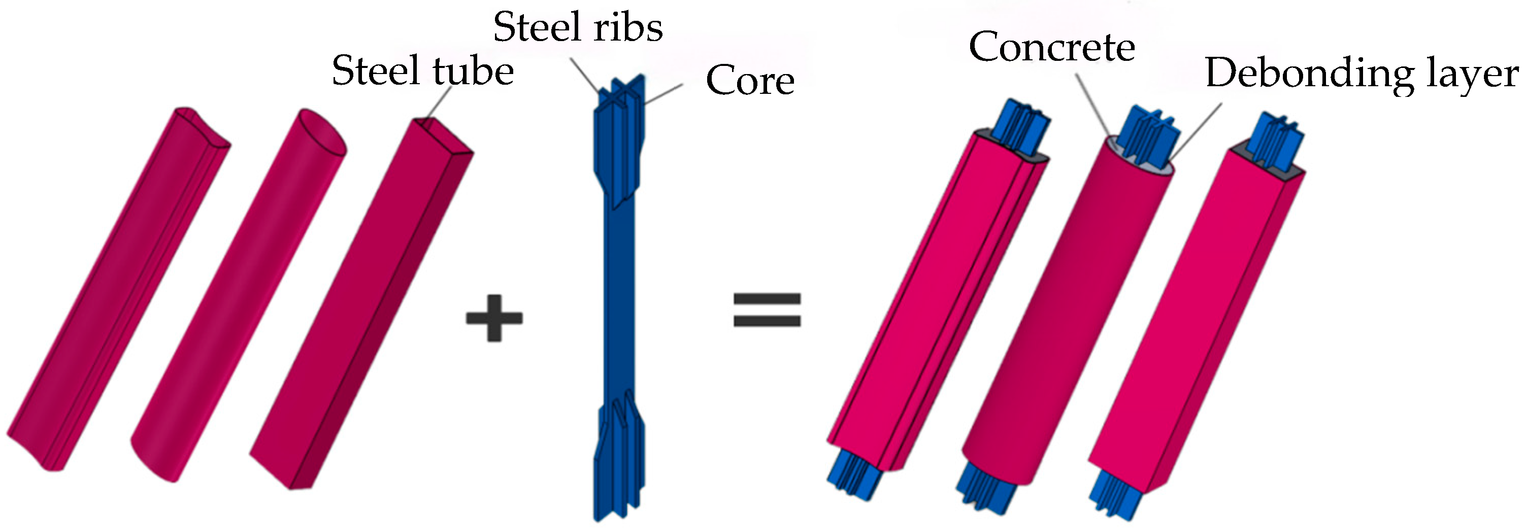
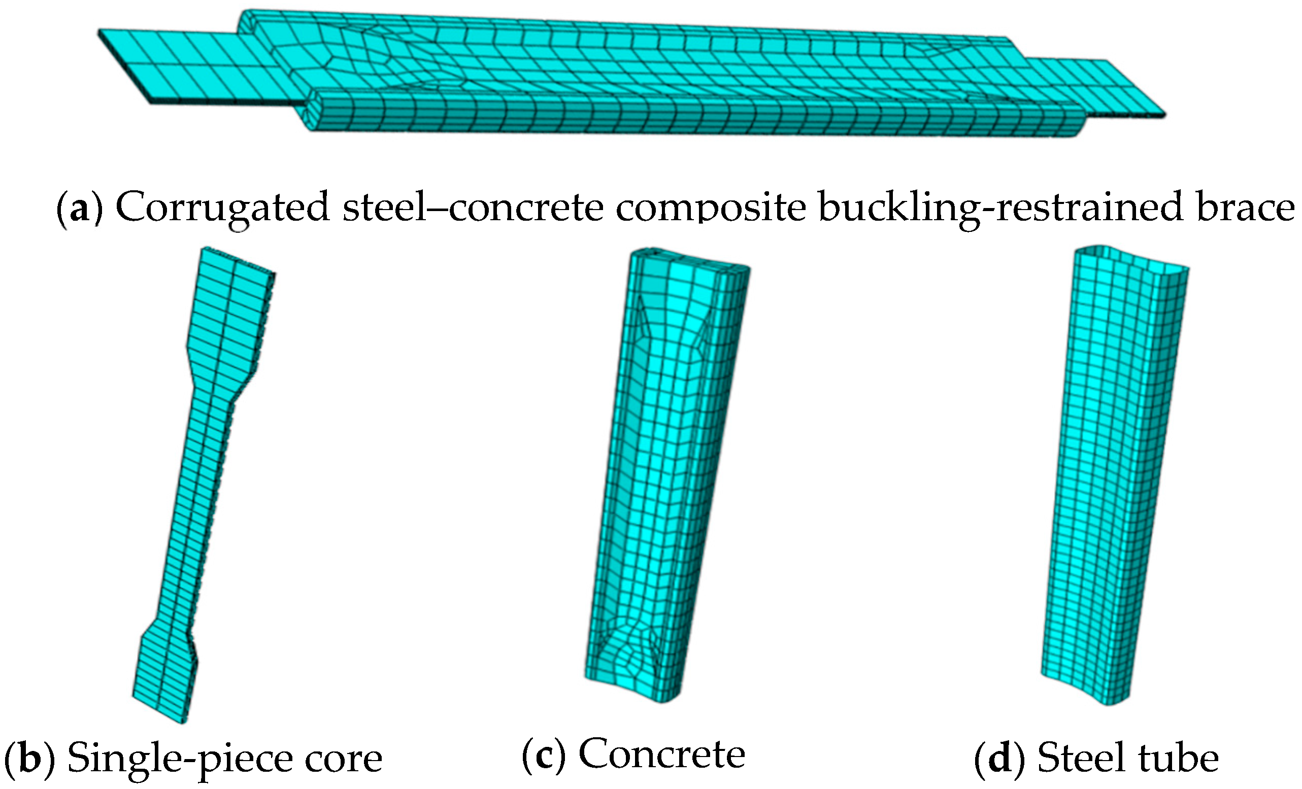
The finite element model of corrugated steel–concrete composite buckling-restrained braces comprises three components: the core steel brace unit, the inner concrete layer, and the outer casing (Figure 1).

The core brace is modeled as a straight-line element. A 2 mm debonding layer is incorporated between the steel and the surrounding concrete to prevent full bonding, thereby avoiding undesirable stress concentrations. The presence of stiffeners introduces geometric complexity to the concrete, complicating mesh generation and potentially influencing simulation accuracy. To simplify the modeling process, the connections between stiffeners and the core brace are merged using an equivalent stiffness approach. Key geometric parameters of the core unit are as follows: total length of 3438 mm, with the energy-dissipating section measuring 160 mm in width and 1600 mm in length, and the connection section measuring 280 mm in width and 594 mm in length; and the uniform thickness is 25 mm.

The modeling process for concrete is similar to that for corrugated steel pipes, employing solid elements for construction with the concrete material specified as C40. Furthermore, the outer casing comprises corrugated steel pipes, manufactured by rolling and welding steel plates into circular or elliptical shapes using rolling machines, followed by corrugation forming via specific equipment. This includes elliptical, rectangular, top-square–bottom-round, pentagonal, and square steel pipes, serving to constrain lateral deformation of the core components.

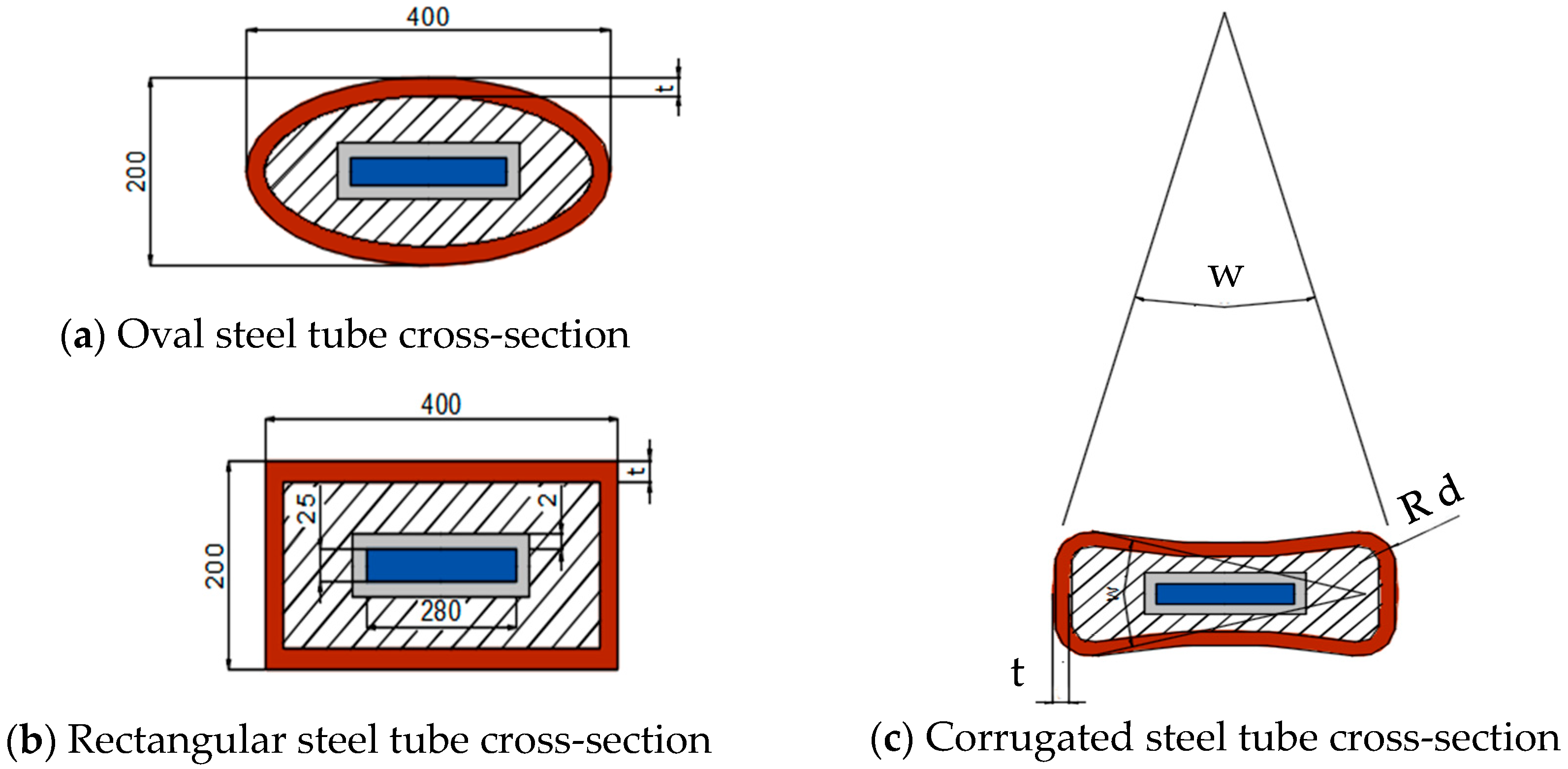
The outer casing is represented using shell elements. Consistent with the corrugated steel pipe manufacturing process and the experimental results reported by Lin [9], the material for the steel casing is defined as Q235, with a total length of 2600 mm. The rectangular casing cross-section measures 400 mm × 200 mm, while the elliptical casing has a major axis radius of 200 mm and a minor axis radius of 100 mm.

In this study, Abaqus software (Dassault Systèmes, Waltham, MA, USA) was used for finite element analysis.

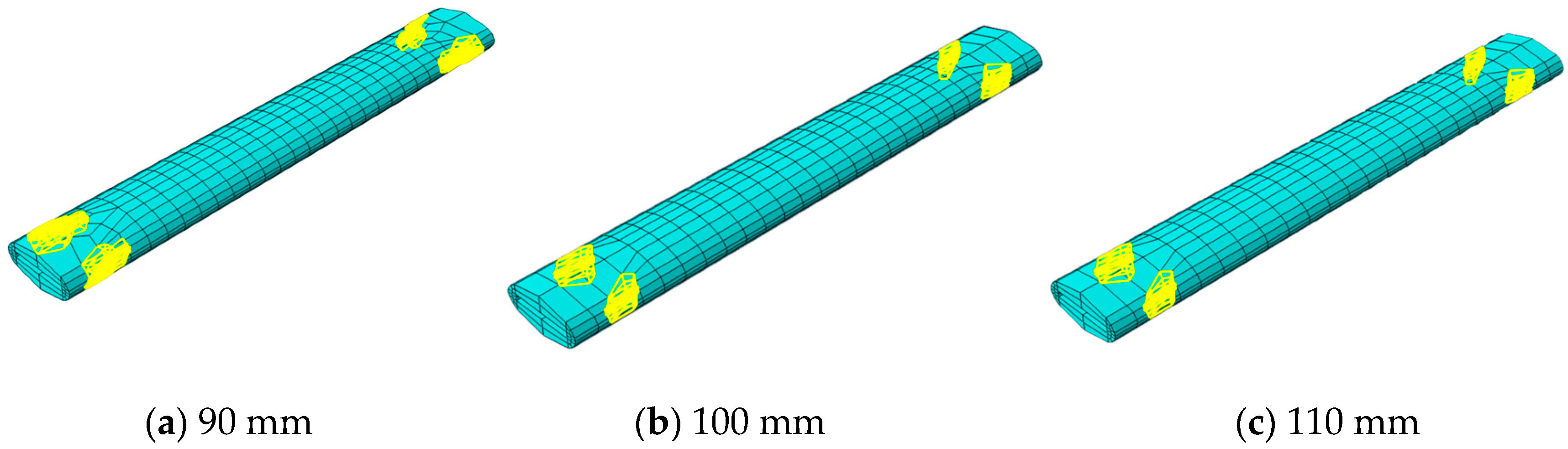
The mesh discretization of the finite element models (Figure 2) critically influences simulation accuracy, convergence behavior, and computational efficiency. Although finer meshes generally improve accuracy, they also increase computational cost and can impede convergence. Through mesh sensitivity analysis, Chen [3] established that a simulation error within 3% indicates a mesh suitable for research purposes. Accordingly, the mesh size was determined based on the cross-sectional characteristics of each model, through iterative refinement of individual components and repeated meshing, accompanied by continuous accuracy checks until predefined criteria were met. Taking the concrete component in Model e-5 as an example: a mesh size of 90 mm resulted in a 5.89% probability of analysis errors; at 100 mm, the error rate dropped to 1.95%; at 110 mm, it increased slightly to 2.13%. Balancing computational efficiency and solution accuracy, a mesh size of 100 mm was adopted for this component. Other parts (e.g., the outer casing and the steel core) did not require the same level of mesh refinement and are meshed using default settings without additional refinement. The mesh configurations for all other models were determined analogously through case-by-case calibration.

The maximum axial load is represented by Py (N), and the yield load is represented by Pm (N).

As the mesh size increases from 90 mm to 110 mm (Figure 3), the maximum axial load (Py) monotonically increases from 9,606,980 N to 10,208,800 N, indicating that mesh refinement leads to a reduction in the peak load. This trend is fully consistent with the observations by Feklistova et al. in their fracture simulations of elastic-brittle bodies, where decreasing element size resulted in lower maximum loads without spontaneous convergence [10]. In contrast, the yield load drops from 5,426,300 N to 5,376,460 N when the mesh size increases from 90 mm to 100 mm, and then remains constant at 100 mm and 110 mm. This suggests that the yield load is less sensitive to mesh size and stabilizes at coarser meshes, while the finer mesh (90 mm) may capture a slightly higher initial yield point due to better resolution of local stress concentrations. The distinct convergence behaviors of these two indicators highlight the necessity of monitoring both load-bearing capacity and yield load in mesh convergence studies to fully assess the reliability of numerical predictions.

As the mesh refines, the location of the first local bulge shifts from the outer weak axis to the outer strong axis. Specifically, at mesh sizes of 110 mm and 100 mm, the bulge occurs on the outer weak axis at similar positions; when the mesh is refined to 90 mm, the bulge location moves to the outer strong axis (still adjacent to the weak-axis side). This indicates that mesh size significantly influences the spatial distribution of the local buckling mode: coarser meshes may suppress or obscure the true buckling pattern, while finer meshes capture the initiation point more accurately.

In addition to load-carrying capacity, the influence of mesh size on energy dissipation was evaluated. The cumulative plastic dissipation energy (ALLPD) at the end of the loading history was extracted for the three mesh configurations (90, 100, and 110 mm) of Model e-5. As summarized in

Table 1. Grid size division.

Mesh Size	90 mm	100 mm	110 mm
Py (N)	9,606,980	10,023,700	10,208,800
The degree of change compared to 100 mm for Py	−4.16%	0%	1.85%
Pm (N)	5,426,300	5,376,460	5,376,460
Total ALLPD (×109 N·mm)	1.22293	1.22297	1.22295
The degree of change compared to 100 mm for total ALLPD	−8.5%	0%	8.3%

, the total ALLPD values are nearly identical, with a maximum deviation of only 0.085% relative to the 100 mm mesh. This confirms that the energy dissipation prediction is essentially mesh-insensitive within the studied range, and the selected mesh size of 100 mm provides reliable results.

The complexity of meshing is primarily governed by the cross-sectional geometry described by three parameters—w, d, and t—all of which are based strictly on the sequential construction of CAD drawings. Here, w denotes the curvature of each side relative to its adjacent corner points; d is the fillet radius at the intersection of two adjacent sides, representing the smoothness of the transition; and t is the thickness of the outer steel tube. The combination of these parameters not only defines the sectional shape of the model but also directly affects the difficulty of meshing. Consequently, for different models, meshing strategies must be tailored according to their specific values of w, d, and t.

A proper definition of mechanical interactions is essential for achieving accurate and convergent solutions. Under cyclic axial loading, the buckling-restrained brace undergoes repeated contact and separation between components. The interaction between the core steel support and the concrete is modeled as surface-to-surface contact, with a friction coefficient of 0.3 in the tangential direction. This value is consistent with the range commonly adopted in finite element analyses of concrete-filled steel tubular structures, where a friction coefficient of 0.35 is frequently used for the steel–concrete interface; accordingly, 0.3 can be regarded as a slightly conservative yet still reasonable engineering choice [11]. A tie constraint is applied between the inner and outer concrete layers to simulate their composite action.

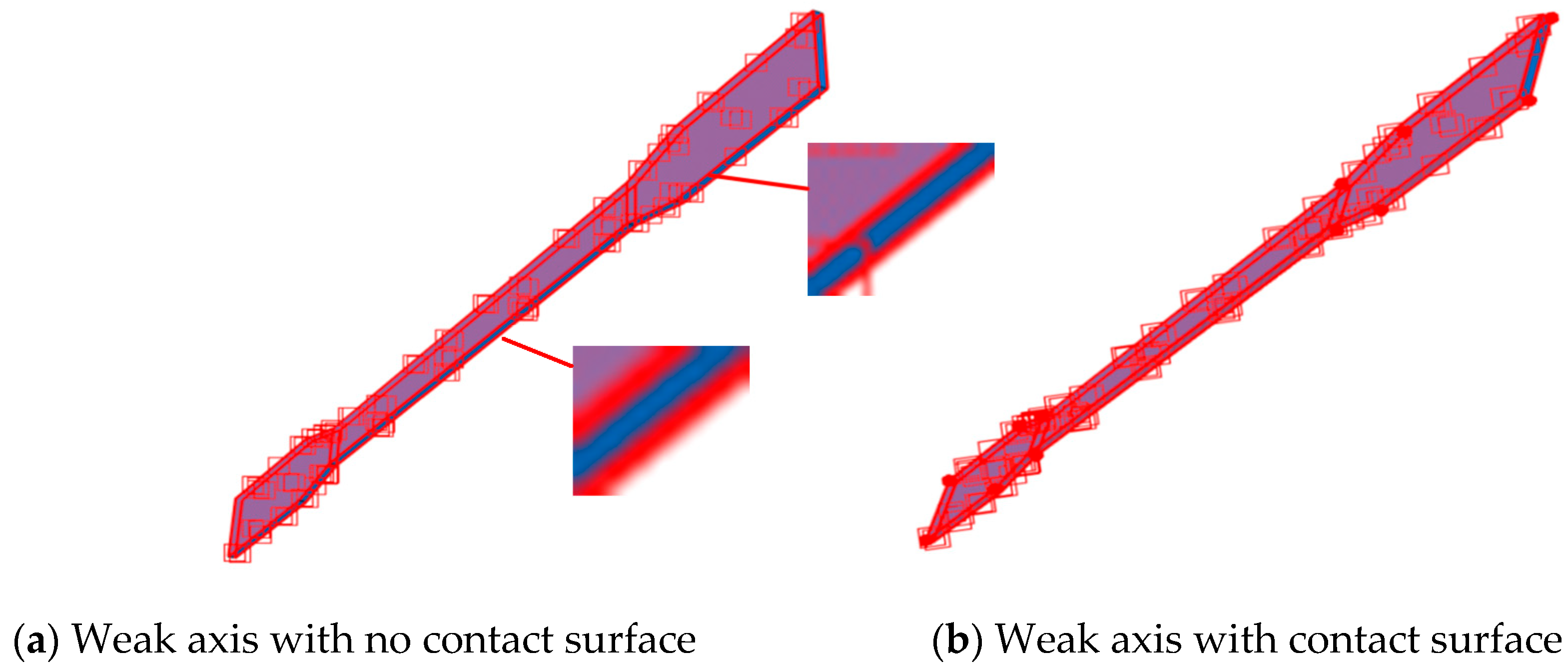
In the contact setup, the normal behavior employs hard contact with allowance for separation after contact, while the tangential behavior defines the maximum elastic slip as 0.005% of the characteristic surface dimension. Based on the mesh size of the model contact surface, the characteristic surface dimension is set to 100 mm (corresponding to the mesh size of the concrete component). Therefore, the maximum elastic slip is calculated as 0.005% × 100 mm = 0.005 mm. The calculations were performed with friction coefficients of 0.2, 0.3, and 0.4 (

Table 2. The influence of the friction coefficient.

Coefficient of Friction	0.2	0.3	0.4
Py (N)	10,211,300	10,023,700	10,210,500
Pm (N)	5,376,460	5,376,460	5,376,460

). The results indicate that the yield load remains unchanged across all three values. The ultimate load capacity exhibits a slight decrease at 0.3, yet the overall fluctuation is less than 1.9%, and the values at 0.2 and 0.4 are nearly identical, showing no monotonic trend. Therefore, within the range of ±0.1, the influence of the friction coefficient on the load-bearing capacity is negligible.

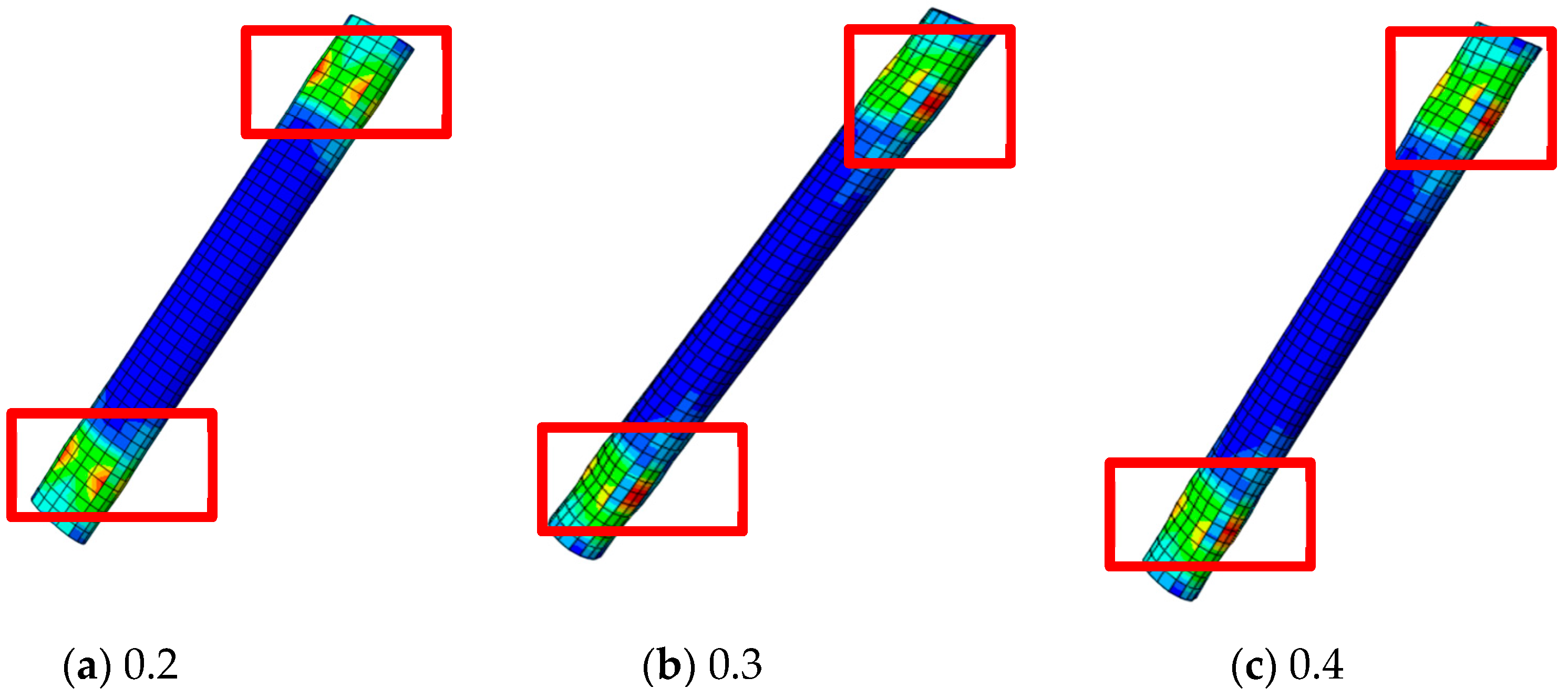
In the Figure 4, the red indicates the maximum stress, while blue indicates the minimum stress. We find that the location of stress concentration shifts progressively toward the weaker axis as the friction coefficient increases.

The finite element model exhibits significant nonlinearity and geometrical complexity, which challenge convergence. The corrugated profile of the steel tube creates an irregular geometry for both the tube itself and the adjacent concrete. Furthermore, the need to accommodate the core brace results in a complex geometry for the inner concrete layer. The presence of a gap between the core brace and the concrete, combined with the cyclic contact-separation process during loading, further complicates the numerical solution.

The initial geometric defect is modeled as a first-order buckling mode with a specified amplitude. In this study, the amplitude is set at L/44 = 78.14 mm/L/55 = 62.51 mm, where L = 3438 mm represents the total length of the component—a value consistent with typical initial defect parameters in steel structures. The buckling mode is derived through eigenvalue buckling analysis and normalized in ABAQUS to ensure the maximum displacement component equals 1.

Table 3. Parameters of the finite element model in this paper.

Number	w (°)	d (mm)	t (mm)	Load Displacement
i-1			12	15 mm, 39 mm, 55 mm
i-2			12	5.4 mm, 9 mm, 18 mm, 30.6 mm, 41.4 mm, 54 mm, 63 mm
r-1	45	45	2	15 mm, 39 mm, 55 mm
r-2	45	45	10	15 mm, 39 mm, 55 mm
r-3	45	45	12	15 mm, 39 mm, 55 mm
r-4	45	45	14	15 mm, 39 mm, 55 mm
r-5	45	40	12	15 mm, 39 mm, 55 mm
r-6	45	55	12	15 mm, 39 mm, 55 mm
r-7	30	45	2	15 mm, 39 mm, 55 mm
r-8	50	45	2	15 mm, 39 mm, 55 mm
r-9	60	45	2	15 mm, 39 mm, 55 mm
r-10	70	45	2	15 mm, 39 mm, 55 mm
r-11	75	45	2	15 mm, 39 mm, 55 mm
e-1			1	22 mm, 44 mm
e-2			4	22 mm, 44 mm
e-3			7	22 mm, 44 mm
e-4			10	22 mm, 44 mm
e-5			12	22 mm, 44 mm
e-6			12	15 mm, 39 mm, 55 mm

presents a comprehensive summary of all finite element models analyzed in this study, categorized by cross-sectional type: rectangular (i-series), corrugated (r-series), and elliptical (e-series). For each model, the table specifies the key geometric parameters—corrugation angle w (in degrees), corner radius d (in mm), and wall thickness t (in mm)—along with the applied displacement loading protocol.

The displacement values listed in the rightmost column (e.g., 15 mm, 39 mm, and 55 mm for most models; 22 mm and 44 mm for e-1 through e-5; and a multi-step protocol for i-2) represent the peak displacement amplitudes imposed during the cyclic loading simulations. These values are critical for understanding the loading history applied to each model:

Overall, 15 mm, 39 mm, and 55 mm correspond to three successive loading steps with increasing displacement amplitudes. These values were selected to cover core strain ranges from approximately 0.94% to 3.44% and the loading displacement is symmetrical at both ends.

For elliptical models e-1 through e-5, a two-step protocol with 22 mm and 44 mm displacements was employed to assess thickness effects under moderate loading conditions.

Model i-2 utilizes a more refined seven-step protocol (5.4 mm, 9 mm, 18 mm, 30.6 mm, 41.4 mm, 54 mm, and 63 mm) to enable detailed investigation of cumulative plastic damage evolution.

The systematic variation in both geometric parameters and loading protocols across these models enables comprehensive parametric analysis of how wall thickness, corner radius, and corrugation angle influence hysteretic behavior, load-bearing capacity, and failure modes under cyclic loading.

It should be noted that this study focused on the hysteresis responses at different amplitudes, but did not conduct a quantitative analysis of cumulative damage effects (stiffness degradation ratio, cumulative energy dissipation, etc.). This will be the main direction of future research.

Let the angle be w (°), the radius of the corner radius be d (mm), and the wall thickness be t (mm) (Figure 5).

Taking the rectangular cross-section of the i-1 model as an example, the steel core has a width (weak-axis direction) b = 400 mm and a thickness (strong-axis direction) h = 200 mm, with a bilinear kinematic hardening model adopted to simulate the material behavior.

The moment of area

$$A=b\times h=400\times 200=\mathrm{80,000} {\mathrm{mm}}^2$$

The moments of inertia about the weak axis

$$I_{\min }={\displaystyle \frac{b{h}^3}{12}}={\displaystyle \frac{400\times {200}^3}{12}}\approx 2.667\times {10}^8 {\mathrm{mm}}^4$$

The moments of inertia about the strong axis

$$I_{\max }={\displaystyle \frac{h{b}^3}{12}}={\displaystyle \frac{200\times {400}^3}{12}}\approx 1.067\times {10}^9 {\mathrm{mm}}^4$$

The weak-axis inertia is defined as a smaller value, while the strong-axis inertia is defined as a larger value.

The yield load Pm under ideal elastoplastic conditions is directly calculated from the cross-sectional area A = b × h and the yield load σ_y.

$$P\mathrm{m}=A\times {\sigma }_y$$

With σ_y = 235 MPa:

$$\mathrm{Pideal}=A\times {\sigma }_y=\mathrm{18,800} \mathrm{KN}$$

For the reported Pm and Py values (Pm ≈ 5376 kN, Py ≈ 8098 kN), the ratios are Pm/Pideal ≈ 28.6% and Py/Pideal ≈ 43.1%, respectively.

In BRB design, the stress of the steel core at the maximum design strain must be estimated via the hardening curve, and due to the confinement effect, the maximum compressive capacity typically exceeds the tensile one. Hence, a compression strength adjustment factor β is introduced, along with the material overstrength factor Ry and strain hardening factor ωy, to determine the maximum compressive capacity Py. Py calculates according to the following formula [12].

$$Py=\beta \times R_y\times {\omega }_y\times Pm$$

In practice, Pm can be identified from the skeleton curve (connecting the peak points of each cycle): the force at the first noticeable nonlinear deviation on the skeleton curve corresponds to the yield load, which in the hysteretic curve can be approximated as the maximum compression value at the end of the first cycle. Meanwhile, Py is directly taken as the absolute maximum tensile or compressive force attained in all cycles, serving as an indicator of the BRB’s ultimate load-bearing capacity.

2.2. Selection of Material Constitutive Models

2.2.1. Steel Material Model

Under seismic loading, the support experiences a small number of hysteresis cycles with large displacement. The commonly employed double-polyline and five-polyline material constitutions in simulations fail to accurately reflect the mechanical behavior of steel under cyclic loading with large deformations [13]. Based on Shi’s [14] investigation into the mechanical properties of Q235 structural steel under cyclic stress, it was found that the Combined Hardening model within the ABAQUS (2020) finite element analysis software effectively simulates metal’s cyclic hardening and Bauschinger effect, accurately reflecting the mechanical behavior of steel under large-deformation cyclic loading.

The Combined Hardening model represents the combined effect of the Isotropic Hardening model and the Kinematic Hardening model. The Isotropic Hardening model posits that yield surfaces undergo uniform contraction within the three-dimensional stress space, being applicable to monotonic loading. The Kinematic Hardening model proposes that yield surfaces undergo rigid translation within the three-dimensional stress space while maintaining consistent dimensions. This model accounts for the von Kisinger effect and effectively simulates the effects of cyclic loading [3]. The Combined Hardening model integrates features of both, positing that the yield surface can undergo contraction and translation in all directions [3].

The growth of plastic strain in the Combined Hardening model is governed by the following equation:

$$\mathrm{F}=\mathrm{f}(\mathsf{\sigma }-\mathsf{\alpha })-{\mathsf{\sigma }}^0=0$$

In the formula, f (σ − α) is the equivalent Mises yield load, S^dev is the deviatoric stress tensor, and α^dev is the deviatoric part of the back stress, which represents the translation of the yield surface center in stress space and is used to describe the Bauschinger effect.

$$\mathrm{f}(\mathsf{\sigma }-\mathsf{\alpha })=\sqrt{{\displaystyle \frac{3}{2}}(S^{dev}-{{\displaystyle \alpha }}^{dev})•(S^{dev}-{{\displaystyle \alpha }}^{dev})}$$

The isotropic hardening portion within the Combined Hardening model determines the size of the yield surface (σ⁰), with its relationship to the equivalent plastic strain defined as follows:

$${\sigma }^0=\sigma {|}_0+Q_{\infty }(1-e^{-b{\epsilon }_{\mathrm{pl}}})$$

σ|₀ is the yield load at zero plastic strain; Q_∞ is the maximum change in the yield surface, reflecting the increase in stress amplitude due to cyclic hardening; b is a parameter controlling the rate of hardening, which determines the saturation rate of the yield surface with respect to the accumulated plastic strain.

The kinematic hardening part is described by the superposition of multiple back stress components.

$$\mathsf{\alpha }={\displaystyle \sum _{\mathrm{k}=1}^{\mathrm{N}}{\mathsf{\alpha }}_{\mathrm{k}}}$$

Each component evolves as follows:

$$\mathsf{\alpha }=C_K{\displaystyle \frac{1}{{{\displaystyle \sigma }}^0}}(\sigma -{\mathsf{\alpha }}_{\mathrm{k}}){{\displaystyle \frac{1}{\epsilon }}}^{pl}-{\gamma }_k{\alpha }_k{{\displaystyle \frac{1}{\epsilon }}}^{pl}$$

In the formula, N is the number of back stress components (N = 4 is adopted to ensure sufficient fitting accuracy); C_k is the initial follower hardening modulus; γ_k is the nonlinear parameter controlling the saturation of back stress with plastic strain development; and ${{\displaystyle \frac{1}{\epsilon }}}^{pl}$ is the equivalent plastic strain rate.

When conducting the parameter analysis in this paper, the parameter settings for the Combined Hardening model were based on the results obtained by Shi et al. [14] and Shu [13] after conducting material property tests on Q235B steel.

The final calibrated material parameters for Q235 steel are as follows. The elastic properties are defined by a Young’s modulus of E = 2.06 × 10⁵ MPa and a Poisson’s ratio of v1 = 0.3. The initial yield load at zero plastic strain, σ|₀, is 235 MPa. For the isotropic hardening component, the parameters are Q_∞ = 45 MPa, which represents the maximum change in the yield surface, and b = 2.5, which controls the rate of hardening. The kinematic hardening behavior is captured by superposing four back stress components (N = 4). The corresponding material constants for each component are: C₁ = 6000 MPa and γ₁= 150; C₂ = 5000 MPa and γ₂ = 120; C₃ = 4000 MPa and γ₃ = 100; and C₄= 3000 MPa and γ₄ = 80.

2.2.2. Concrete Material Model

The concrete is modeled using the Concrete Damaged Plasticity (CDP) model in ABAQUS, which is suitable for simulating the mechanical behavior of concrete under cyclic and dynamic loading [3]. The compressive skeleton curve is based on the Popovics model [15] and is modified to account for the confinement effect of the steel tube; the tensile softening behavior is described using a stress–crack opening strain relationship. This study takes C40 concrete as an example, with a cubic compressive strength of f_cu = 40 MPa. The complete parameter definitions and an illustrative calculation are provided below (

Table 4. Elastic parameter.

Parameter	Value	Unit
Young’s modulus Ec	30,000	MPa
Poisson’s ratio ν2	0.2	-

and

Table 5. CDP parameters.

Parameter	Value	Unit
Dilation angle ψ	20	°
Eccentricity ϵ	0.1	-
Ratio of biaxial to uniaxial compressive strength fb0/fc0	1.16	-
Second stress invariant ratio Kc	0.667	-
Viscosity parameter μ	0.0005	-

).

For the compressive concrete constitutive model, researchers [16,17,18,19] proposed an improved model:

$$y=\frac{Ax+(B-1)x^2}{1+(A-2)x+B{x}^2}$$

$$y=\frac{{\sigma }_c}{f_{cc}}$$

$$x=\frac{{\epsilon }_c}{{\epsilon }_{cc}}$$

The f_cc and ε_cc represent the compressive strength and peak strain of the restrained concrete, respectively, and constraint adjustment parameter ξ = 5.0 [16], calculated using the following formula:

$${\epsilon }_{cc}={\epsilon }_{co}(1+{\displaystyle \frac{f_r}{f_{co}}}\cdot \xi )$$

$$f_{cc}=f_{co}+k_0\cdot f_r$$

In the formula, f_co denotes the compressive strength of unreinforced concrete (with f_cu = 40 MPa), where f_co = 0.76, f_cu = 30.4 MPa; ε_co represents the peak strain of unreinforced concrete; f_r is the effective restraint stress, accounting for both corrugation patterns and wall thickness effects; and k₀ is the restraint efficiency coefficient.

The peak strain of unreinforced concrete:

$${\epsilon }_{co}=0.7{(f_{co})}^{0.31}\cdot {10}^{-3}$$

If f_co = 30.4 MPa, the ε_co = 2.02 × 10⁻³.

The modulus of elasticity:

The secant modulus:

$$E_{\sec }={\displaystyle \frac{f_{cc}}{{\epsilon }_{cc}}}$$

$$E_c=5000\sqrt{f_{cu}}=5000\cdot \sqrt{40}=\mathrm{31,623} \mathrm{MPa}$$

Based on the above peak points, a complete stress–strain relationship was generated using the Popovics form of the skeleton curve, and was converted into the yield load-non-elastic strain data required for the ABAQUS CDP model, as shown in Table 3. The first row in the table corresponds to the initial yield point (with non-elastic strain of 0), the third row represents the peak point (40.0 MPa @ non-elastic strain 0.0011576), and the subsequent rows represent the softening section.

Example calculation (using corrugated steel pipe-reinforced concrete as a case study): Effective restraint stress f_r = 4.5 MPa, with a restraint efficiency coefficient k₀ = 1.2.

$$f_{cc}=30.4+1.2\times 4.5=35.8 \mathrm{MPa}$$

$$E_{\sec }={\displaystyle \frac{31.4}{0.00232}}=\mathrm{13,534} \mathrm{MPa}$$

$${\epsilon }_{cc}=2.02\times {10}^{-3}\times (1+{\displaystyle \frac{4.5}{30.4}}\times 5)=3.51\times {10}^{-3}$$

The input data of compressive stress–non-elastic strain listed in

Table 6. Input data for stress behavior.

Yield Stress (MPa)	Inelastic Strain
0.79598	0
30.0	0.00024118
40.0	0.001157587
36.0	0.003800003
31.0	0.006486247
26.0	0.009146676
23.0	0.011783124
21.0	0.014402941
18.0	0.01701214

is based on the peak point of the aforementioned constrained concrete (f_cc = 35.8 MPa, ϵ_cc = 0.003515). After generating a complete stress–strain relationship using the Popovics form of the skeleton curve, it is then converted into non-elastic strain through the following formula:

$${\epsilon }_{incel}={\epsilon }_{total}-{\displaystyle \frac{\sigma }{{\mathrm{E}}_{\mathrm{c}}}}$$

The third row of Table 6 (40.0 MPa @ inelastic strain 0.0011576) corresponds to the peak point of unrestrained concrete, which is used to define the initial yield surface in the CDP model. The peak strength f_cc of restrained concrete is indirectly reflected in the definition of the compressive damage parameter and simulates the restraint effect through damage evolution.

The tensile strength of concrete is calculated as follows:

$$f_t=0.26\times {\left(f_{cu}\right)}^{2/3}$$

With f_cu = 40 MPa:

$$f_t=0.26\times {\left(f_{cu}\right)}^{2/3}=0.26\times {40}^{2/3}=3.04 \mathrm{MPa}$$

The peak tensile strain is calculated as follows:

$${\epsilon }_t=65\times {10}^{-6}\times {f_t}^{0.54}=65\times {10}^{-6}\times {3.04}^{0.54}=1.16\times {10}^{-4}$$

Linear softening is one of the widely used stretching softening models [20]. The linear softening is adopted for the tensile softening segment, and the softening modulus is taken as E_ts = 0.1 E_c [20], where the tensile data is based on strain.

Both the compressive and tensile damage (

Table 7. Tensional force as input data.

Yield Stress (MPa)	Crack Strain
0.82994081	0
3.4586835	3.27 × 10−5
1.2122085	0.000257269
0.6898757	0.000423833
0.49436852	0.000579379
0.39207116	0.000731768
0.32866448	0.000882826
0.28519805	0.001033191
0.25335558	0.001183143
0.22890855	0.001332824

and

Table 8. Compressive damage input data.

Damage Parameter dc	Inelastic Strain
0	0
0.130458915	0.00024118
0.136844943	0.001157587
0.56580698	0.003800003
0.737657565	0.006486247
0.814491898	0.009146676
0.857041437	0.011783124
0.883898342	0.014402941
0.902347918	0.01701214

) are based on the energy equivalence hypothesis. The relationship between the damage parameter dd and the stress and inelastic strain is defined as follows:

The compressive damage parameter dc is defined, and it is input in tabular form (Table 8).

The tensile damage parameter dt is defined similarly, based on the cracking strain (

Table 9. Tensile damage input data.

Tensile Damage Parameter dt	Cracking Strain
0	0
0.009890894	3.27 × 10−5
0.589625097	0.000257
0.747783867	0.000424
0.815250437	0.000579
0.852905746	0.000732
0.877092164	0.000883
0.894020959	0.00103
0.906577092	0.00118
0.916286803	0.001332824

).

The compressive damage parameter dc and tensile damage parameter dt are defined based on the energy equivalence hypothesis, combined with stress–strain curves calibrated from design codes.

For damage factor calculation, using the energy equivalence hypothesis, the damage variable is derived from the ratio of the damaged elastic modulus to the initial undamaged modulus:

$$d_c=1-\sqrt{{\displaystyle \frac{{\sigma }_c}{{\mathrm{E}}_{\mathrm{c}}\cdot {\epsilon }_{\mathrm{c}}}}}$$

where σ_c and ϵ_c are the compressive stress and total strain at a given point on the descending branch.

Similarly, the tensile damage parameter dt is computed as:

$$d_t=1-\sqrt{{\displaystyle \frac{{\sigma }_t}{{\mathrm{E}}_{\mathrm{c}}\cdot {\epsilon }_{\mathrm{t}}}}}$$

With σ_t and ϵ_t being the tensile stress and total strain in the softening regime.

In the concrete damaged plasticity model, stiffness recovery is governed by the compression recovery factor and the tension recovery factor. In this study, the compression recovery factor is set to wc = 1, indicating full recovery of compressive stiffness upon crack closure, while the tension recovery factor is taken as wt = 0, implying that tensile stiffness does not recover after cracking, and these apply in the whole analysis.

However, in the CDP model of ABAQUS, the damage is typically set to zero at the peak stress to maintain an undamaged unloading stiffness before softening begins. In practical numerical simulations, a small non-zero damage value is often assigned at the peak point to improve convergence while still capturing the onset of micro-cracking. Therefore, in Table 8, the damage value at the peak point is taken as 0.1368 (slightly above zero), a common practice adopted in [3,20] that balances numerical stability and physical consistency.

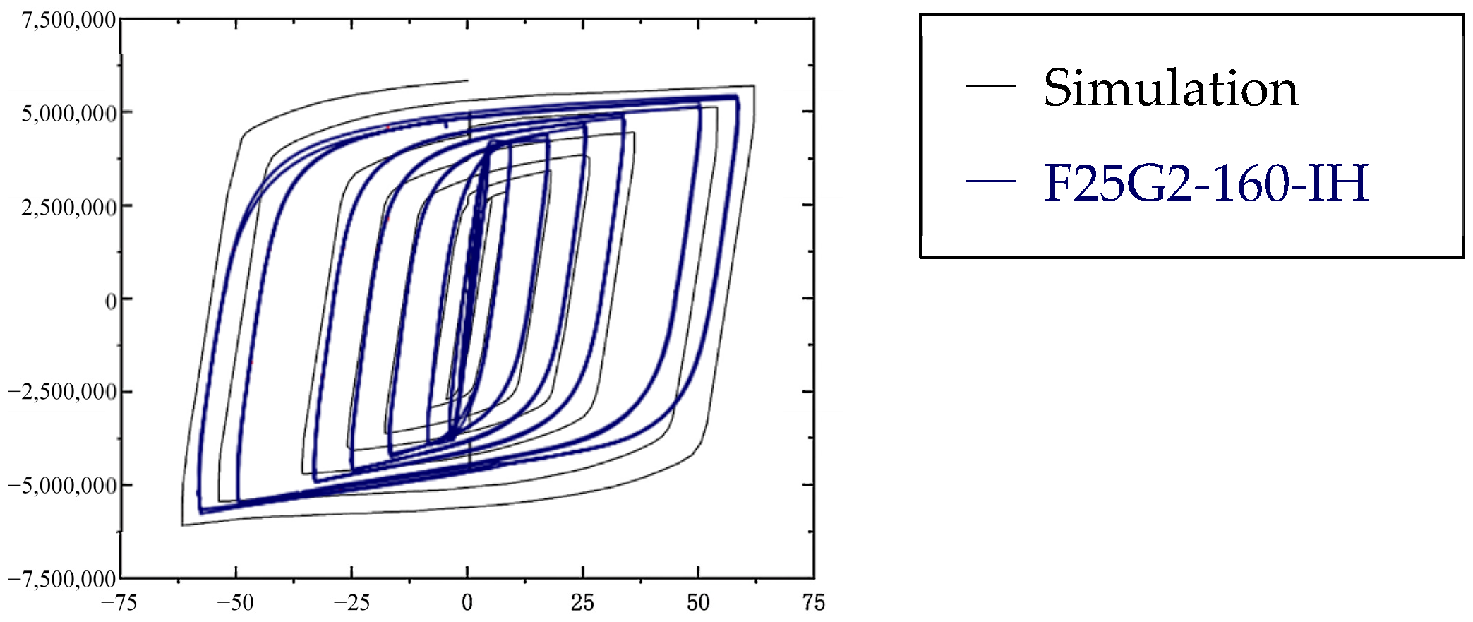
To validate the accuracy of the calibrated combined hardening model parameters for Q235 steel, a single-element model in ABAQUS was used to replicate the cyclic loading response of the F25G2-160-IH specimen from the thin-profile BRB tests by Lin et al. [9]. The simulated hysteresis curve was compared with the digitized experimental curve. After normalization by the core length Lc = 1800 mm and the yield load Py = 4162 kN, the simulated curve showed good agreement with the experimental hysteresis loop extracted from Lin et al. (Figure 6), accurately capturing the Bauschinger effect and cyclic hardening characteristics of the steel. Quantitative error metrics indicated a root mean square error (RMSE) of 0.042, a relative error of 2.3% for the peak tensile force, and 3.1% for the peak compressive force, all within acceptable ranges. These results confirm the reliability of the calibrated parameters in describing the cyclic constitutive behavior of Q235 steel.

2.3. Finite Element Analysis Comparison

2.3.1. Model Variables

For wall thickness, while maintaining other parameters constant, the effect of wall thickness variations (

Table 10. Elliptical finite element model parameters.

Number	t (mm)	Py (N)	Local Bulging Observed
e-1	1	5,736,720	No
e-2	4	6,415,350	No
e-3	7	9,062,490	No
e-4	10	9,141,280	No
e-5	12	10,023,700	No
e-6	12	9,428,560	Yes

and

Table 11. Parameters related to wall thickness of corrugated steel tubes.

Number	w (°)	d (mm)	t (mm)	Py (N)	Local Bulging Observed
r-1	45	45	2	7,900,156	No
r-2	45	45	10	8,039,110	No
r-3	45	45	12	8,049,170	No
r-4	45	45	14	8,138,400	No

) on the hysteretic behavior of the corrugated section was analyzed. Based on the established research parameters, the hysteresis curve of buckling-restrained braces with different wall thicknesses can be determined.

Elliptical Sections: For elliptical cross-sections, increasing wall thickness from 1 mm to 12 mm produces a monotonic and substantial increase in load-bearing capacity, from 5.74 MN (e-1) to 10.02 MN (e-5)—a 75% improvement. Notably, all elliptical models remained stable with no observed local buckling throughout the thickness range. The examination of the corresponding hysteresis curves (Figure 7) reveals a progressive enhancement in hysteretic behavior: The e-1 model exhibits a noticeably less full hysteresis loop compared to its thicker counterparts, indicating relatively lower energy dissipation capacity. As thickness increases to 4 mm (e-2), 7 mm (e-3), 10 mm (e-4), and finally 12 mm (e-5), the hysteresis curves become increasingly full and stable, with e-5 demonstrating the most favorable energy dissipation characteristics. This monotonic improvement can be attributed to the enhanced flexural stiffness of the elliptical tube, which provides progressively greater confinement to the core concrete, delays steel yielding, and maintains stable composite action under cyclic loading.

Based on the geometric parameters of the elliptical section with a major axis a = 400 mm and a minor axis c = 200 mm, the diameter-to-thickness ratio D/t is defined using the minor axis cc as the characteristic dimension D. As the diameter-to-thickness ratio monotonically decreases from 200/1 = 200 (e-1, wall thickness 1 mm) to 200/12 ≈ 16.7200/12 ≈ 16.7 (e-5, wall thickness 12 mm), the load-bearing capacity of the specimens continuously increases from 5.74 MN to 10.02 MN, an improvement of 75%. Throughout the entire range of diameter-to-thickness ratios, all elliptical models remained stable with no occurrence of local buckling.

The evolution of hysteretic performance is positively correlated with the load-bearing capacity: as the diameter-to-thickness ratio decreases, the fullness of the hysteresis curves progressively improves. The e-1 model with the largest diameter-to-thickness ratio (D/t = 200) exhibits significant pinching in its hysteresis loops and relatively low energy dissipation capacity. As the diameter-to-thickness ratio decreases successively to 50 (e-2), 28.6 (e-3), 20 (e-4), and 16.7 (e-5), the hysteresis loops gradually become fuller and more stable, with the e-5 model demonstrating the most favorable energy dissipation characteristics. This monotonic improvement stems from the enhanced flexural stiffness of the elliptical tube as wall thickness increases: a smaller diameter-to-thickness ratio provides stronger confinement to the core concrete, delays steel yielding, and maintains stable composite action. Simultaneously, the inherent smoothness of the elliptical geometry promotes uniform stress distribution, allowing the additional material to be utilized efficiently while avoiding instability.

The elliptical geometry’s inherent smoothness facilitates uniform stress distribution, allowing additional material to be efficiently utilized without triggering instability.

In addition to geometric parameters, the loading protocol also significantly influences the buckling behavior of BRBs. A comparison between Models e-5 and e-6, which share identical geometric parameters (wall thickness of 12 mm) but are subjected to different displacement loading histories, illustrates this effect. Model e-5 was cycled under two displacement amplitudes (22 mm and 44 mm) and did not exhibit local bulging. In contrast, Model e-6, which experienced larger displacement amplitudes (15 mm, 39 mm, and 55 mm), eventually developed local bulging. This comparison indicates that, even with identical geometric configurations, a more demanding loading protocol—characterized by larger displacement amplitudes and a greater number of cycles—can trigger local instability, thereby compromising the load-bearing capacity and energy dissipation stability of the member. Therefore, in practical engineering design, attention should be paid not only to geometric optimization but also to the intensity and number of cycles of seismic inputs when evaluating BRB performance.

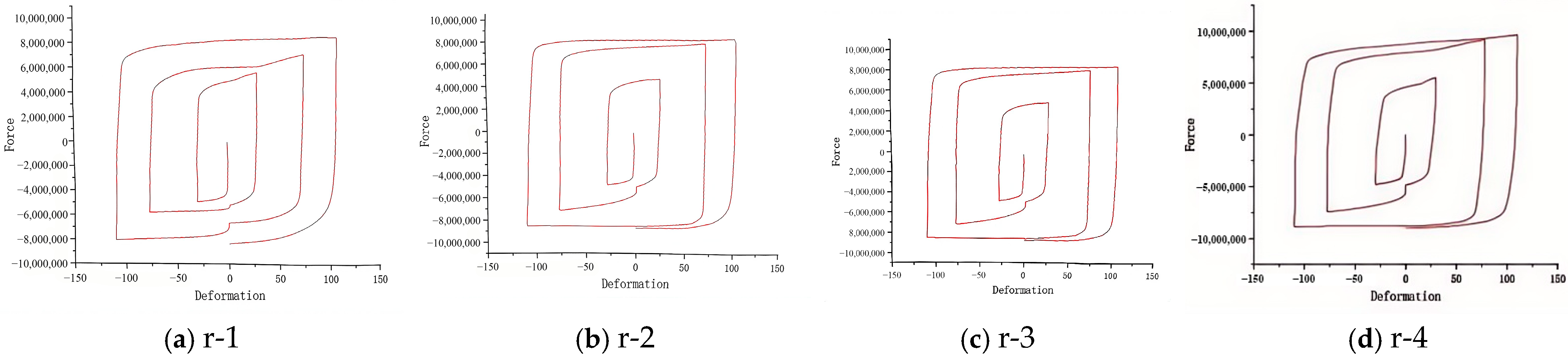
Corrugated Sections: The corrugated sections exhibit a distinctly different trend. In Figure 8, a wall thickness increase from 2 mm (r-1, 7.90 MN) to 10 mm (r-2, 8.04 MN) yields a 1.7% improvement in capacity, with further thickening to 12 mm (r-3, 8.05 MN) and 14 mm (r-4, 8.14 MN) producing still marginal gains (less than 1.5% additional improvement from r-2 to r-4). This diminishing returns phenomenon indicates that the additional material contributes primarily to elastic stiffness rather than ultimate capacity enhancement.

The corresponding hysteresis curves are as follows:

Remarkably, the hysteresis curve evolution for corrugated sections contradicts intuitive expectations. Unlike elliptical sections, where thicker walls consistently improve hysteretic behavior, the corrugated models show a progressive degradation in hysteresis loop fullness with increasing thickness. The Model r-1 (2 mm) displays the most full hysteresis characteristics, while Models r-2 (10 mm), r-3 (12 mm), and r-4 (14 mm) exhibit increasingly pinched and less well-stacked loops. This counterintuitive phenomenon requires careful mechanical interpretation.

The superior hysteretic performance of thinner corrugated tubes (r-1) can be explained by their greater flexibility, which allows the corrugated geometry to accommodate cyclic deformations through distributed bending rather than localized stress concentrations. The thin wall permits the corrugations to act as “flexural hinges,” distributing plasticity across a larger volume and maintaining stable energy dissipation. As wall thickness increases, the corrugated tube becomes progressively stiffer, suppressing this beneficial flexural mechanism and forcing deformation to concentrate at geometric discontinuities—particularly at the corrugation peaks and valleys. This stress concentration effect, combined with the inherent geometric complexity of corrugated profiles, leads to an earlier onset of localized damage mechanisms that manifest as pinched hysteresis loops, despite the modest increase in ultimate capacity.

Synthesis and Design Implications: The contrasting behaviors between elliptical and corrugated sections reveal a fundamental principle: optimal material utilization requires matching geometric form to thickness-dependent mechanical behavior. Elliptical sections, with their smooth, continuous curvature, efficiently convert additional material into enhanced performance across the entire thickness range studied. Corrugated sections, conversely, exhibit a trade-off: moderate thickness (2–10 mm) leverages the geometric flexibility for superior hysteretic performance, while thicknesses beyond the critical threshold (≥10 mm) sacrifice energy dissipation capacity for marginal gains in ultimate strength.

The “critical thickness” concept thus extends beyond mere capacity considerations to encompass hysteretic performance. For corrugated sections, the optimal design range for seismic applications may lie below the thickness that maximizes ultimate capacity, prioritizing the well-stacked hysteresis loops essential for energy dissipation over minor strength enhancements. This finding aligns with Zeng et al. [21], who observed that relatively thin plates exhibit stiffness degradation but maintain energy dissipation, while excessively thick sections within certain ranges produce well-stacked but potentially over-conservative designs. The present study quantifies this trade-off, providing engineers with actionable guidance for balancing strength, stability, and seismic performance in non-rectangular BRB design.

This investigation explores the influence of corner radius on the hysteretic behavior of corrugated steel–concrete composite buckling-restrained braces. The analysis is performed while maintaining consistent wall thickness and angle, based on the established research parameters. The impact of the corner radius on the structural performance, including maximum axial load and buckling states.

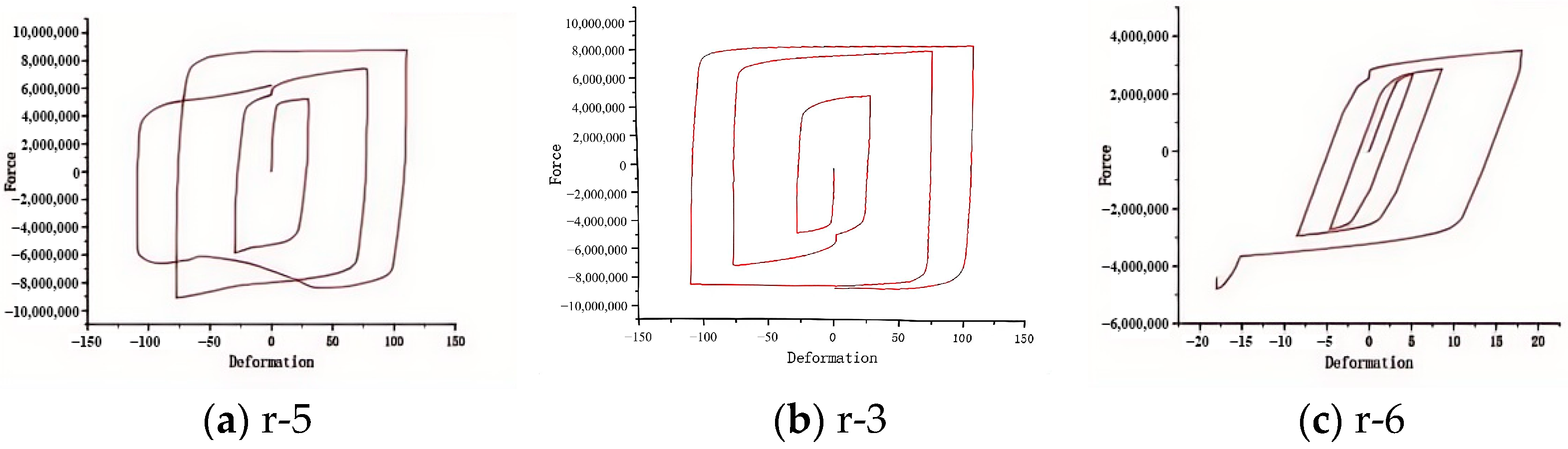
The corner radius parameter d exerts a profound and non-monotonic influence on both the load-bearing capacity and the hysteretic behavior of corrugated steel–concrete composite BRBs (

Table 12. Parameters related to the corner radius of corrugated steel tubes.

Number	w (°)	d (mm)	t (mm)	Py (N)	Local Bulging Observed
r-5	45	40	12	8,558,580	Yes
r-3	45	45	12	8,049,170	No
r-6	45	55	12	10,572,100	Yes

, Figure 9). Three distinct behavioral patterns emerge as the corner radius varies from 40 mm to 55 mm while the wall thickness (t = 12 mm) and the corrugation angle (w = 45°) are kept constant.

Reducing the corner radius from the baseline value of 45 mm to 40 mm increases the peak load capacity from 8.05 MN to 8.56 MN (an improvement of 6.3%). This gain, however, is achieved at the expense of local stability, as the model exhibits localized bulging. The corresponding hysteresis curve (Figure 9a) displays an irregular shape with pronounced distortions: abrupt changes in slope and uneven force development occur during the cycles, indicating unstable energy-dissipation behavior. From a mechanical perspective, this irregularity can be explained by the sharper corner radius, which introduces a geometric discontinuity that acts as a stress raiser; consequently, plastic deformation concentrates at the corners instead of being distributed uniformly along the corrugated profile. Although this stress concentration triggers premature local buckling, as evidenced by the observed bulging, it also engages a larger portion of the cross-section in plastic deformation before global failure occurs, thereby temporarily enhancing the peak capacity. Nevertheless, this localized mechanism produces an erratic hysteretic response and compromises the BRB’s ability to dissipate energy reliably over many cycles.

Model r-3, with the baseline corner radius of 45 mm, exhibits no local bulging and reaches a peak capacity of 8.05 MN. Among all corner-radius variants, it demonstrates the most favorable hysteretic characteristics. Its hysteresis curve (Figure 9b) is remarkably full and regular; the loading branches transition smoothly, and the force development remains stable throughout each cycle. Such a full shape reflects excellent energy-dissipation capacity, minimal pinching, and consistent cyclic-hardening behavior. The mechanical explanation lies in the geometric harmony achieved at this radius: 45 mm provides sufficient smoothness to avoid severe stress concentrations while retaining enough curvature to ensure effective load transfer between the steel tube and the concrete. This configuration allows the corrugated profile to function as intended—distributing plasticity across the entire section rather than concentrating it at geometric discontinuities.

Increasing the corner radius to 55 mm yields the highest peak capacity among all variants (10.57 MN, a 31% increase over the baseline). Paradoxically, however, this configuration triggers local bulging and highly irregular hysteretic behavior. The hysteresis curve (Figure 9c) is severely distorted: it exhibits sharp peaks, abrupt force drops, and asymmetric loops that deviate markedly from an ideally full shape. This seemingly contradictory outcome—enhanced capacity accompanied by instability and an irregular response—reveals a fundamental mechanical principle. The larger radius improves the initial load-transfer mechanism by reducing stress concentrations at the corners, thereby allowing a more uniform confinement distribution and delaying the onset of plasticity. Consequently, the section can attain a higher peak load before failure. Yet, once local buckling initiates, the larger radius creates a more abrupt geometric transition in the post-buckling regime, which leads to an unstable force-displacement response. The irregular hysteresis reflects this instability: the structure undergoes sudden stiffness changes and load redistributions during cycling, and despite its impressive ultimate capacity, it cannot sustain stable energy dissipation.

The analysis of the corner radius demonstrates that optimal seismic performance requires more than merely maximizing the peak capacity; a balanced configuration that ensures a stable hysteretic response throughout the entire loading history is essential. For the geometry studied, the baseline 45 mm radius represents such an optimum: it trades a moderate capacity (8.05 MN) for the reliable, full hysteretic behavior that is indispensable for earthquake energy dissipation. Both the reduced-radius and increased-radius configurations, despite reaching higher peak loads, exhibit irregular hysteresis and local instability. Such behavior would compromise performance in actual seismic events, where multiple cycles and stable energy dissipation are critical.

The selection of a corner radius must consider not only the ultimate strength but also the stability of the cyclic response. The 45 mm configuration shows that a moderate geometric transition provides the mechanical continuity necessary for stable composite action, whereas extremes in either direction—whether too sharp or too generous—create conditions that promote irregular behavior. Engineers should therefore prioritize configurations that yield full hysteresis loops over those that achieve only marginal gains in peak capacity at the expense of cyclic stability.

The effect of angle on hysteretic behavior was examined under constant corner radius and wall thickness. Yield stress and buckling states were evaluated for different arc radii using the established parametric set (

Table 13. Parameters related to the angle of corrugated steel tubes.

Number	w (°)	d (mm)	t (mm)	Py (N)	Local Bulging Observed
r-7	30	45	2	8,315,410	No
r-1	45	45	2	7,900,156	No
r-8	50	45	2	7,342,400	Yes
r-9	60	45	2	9,758,640	Yes
r-10	70	45	2	6,489,880	Yes
r-11	75	45	2	6,539,420	Yes

).

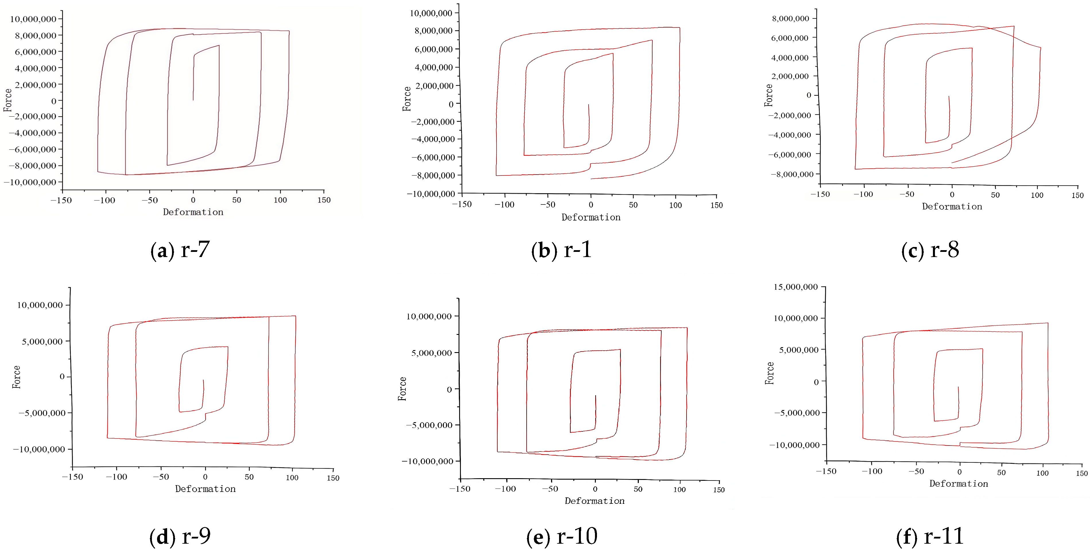
The corresponding hysteresis curves (Figure 10) are as follows:

Moderate Angles (30–45°, Models r-7 and r-1): At 30° (r-7), the structure remains stable with no local buckling and achieves a relatively high peak capacity of 8.32 MN. Its hysteresis curve (Figure 10a) is moderately full, indicating acceptable energy dissipation, yet it is not as full as the 45° configuration. From a mechanical perspective, the shallower corrugation at 30° produces a stiff and compact cross-section. While this stiffness enhances the initial load-bearing capacity and prevents buckling, it also restricts the spread of plasticity; deformation tends to concentrate in a smaller region, thereby reducing the overall hysteretic energy dissipation. As the angle increases to 50° (r-8), the peak capacity drops notably to 7.34 MN; however, the 45° (r-1) bearing capacity was higher than that of the r-8, and the hysteresis curve becomes remarkably full and regular (Figure 11), being the fullest among all angle variants and exhibiting excellent energy-dissipation capacity with minimal pinching and stable cyclic hardening. The 45° configuration appears to represent a geometric optimum: the corrugation provides sufficient flexibility to allow distributed plasticity without triggering premature instability. Within this moderate angle range, a clear trade-off exists between load-bearing capacity and hysteretic performance: 30° favors strength, whereas 45° favors energy dissipation.

At 50° (r-8), the hysteresis curve (Figure 10) exhibits pronounced irregularities—sharp peaks and abrupt force drops—indicating unstable energy-dissipation behavior. This irregularity originates from the onset of buckling: the increased corrugation angle introduces geometric discontinuities that create stress concentrations, triggering local instability and leading to an erratic post-buckling response.

At 60° (r-9), despite the presence of local buckling, the peak capacity reaches the maximum among all angle variants (9.76 MN). Remarkably, its hysteresis curve (Figure 10) is much fuller and more regular than that of r-8, approaching the fullness of the 45° configuration while delivering substantially higher capacity. This counterintuitive improvement can be explained by a change in the buckling mode: at 60°, the corrugation geometry may promote multi-wave local buckling that distributes plasticity over a larger volume, thereby enabling stable post-buckling energy dissipation. The increased angle enhances the mechanical interlock between the steel tube and concrete, improving composite action, while the greater deformation capacity allows the section to sustain higher loads before failure. Thus, 60° represents a “sweet spot” where geometric optimization simultaneously elevates strength and restores hysteretic quality.

Large Angles (70–75°, Models r-10 and r-11): Beyond 60°, further increases in angle lead to a decline in peak capacity: 70° yields 6.49 MN and 75° yields 6.54 MN, both accompanied by local buckling. Surprisingly, the hysteresis curves for these angles (Figure 10) are noticeably fuller than that of r-8, and in fact become progressively fuller as the angle increases from 70° to 75°. This trend suggests that at very large corrugation angles, the buckling mode may evolve into a more distributed pattern—possibly involving multiple half-waves—that, although initiated earlier, allows more uniform plastic straining and thus improves energy dissipation. However, the overall stiffness reduction caused by the exaggerated geometry outweighs any benefit from the altered buckling mode, resulting in lower ultimate capacities. The hysteresis curves, while relatively full, still exhibit some residual irregularities, indicating that the post-buckling response is not perfectly stable.

The angle analysis demonstrates that the corrugation angle profoundly influences not only the load-bearing capacity but also the stability and quality of the hysteretic response. A single metric—peak capacity—is insufficient to characterize seismic performance. The 45° configuration offers the most reliable energy dissipation, making it ideal for applications where dependable cyclic behavior is paramount. The 60° configuration, by contrast, achieves the highest strength while maintaining reasonably good hysteretic quality, representing a balanced choice for designs that prioritize both capacity and energy dissipation. Angles below 45° provide stable behavior but at the cost of reduced hysteretic efficiency, while angles above 60° sacrifice strength for modest gains in hysteretic fullness. Engineers must therefore carefully weigh these trade-offs and select the angle that best aligns with the specific performance objectives of the structure.

There is a significant coupling effect between the angle (w) and the corner radius (d), which together determine the stability boundary of the structure. Taking d = 45 mm as a benchmark, when the angle deviates from 45°, local bulging is induced even with a wall thickness of only 2 mm. Similarly, fixing the angle at 45° while reducing the corner radius to 40 mm or increasing it to 55 mm also leads to instability. This indicates that the stable region may be concentrated within a narrow band centered around (45°, 45 mm).

The effect of wall thickness (t) depends on this geometric foundation. Under a stable geometric combination (such as (w = 45°, d = 45 mm)), increasing the wall thickness steadily enhances the load-bearing capacity without inducing bulging. However, under inherently unstable geometric conditions (such as (w = 60°, d = 45 mm) or (w = 45°, d = 40 mm)), local bulging still occurs even when the wall thickness is increased to 12 mm. This suggests that geometric instability plays a dominant role; while wall thickness can influence the magnitude of the load capacity, it cannot fully suppress the occurrence of buckling.

This leads to a central trade-off: certain geometric combinations (such as (w = 60°, d = 45 mm, t = 2 mm)) can achieve a relatively high ultimate load capacity even in an unstable state, but this high capacity is often accompanied by bulging, which may compromise the ductility and energy dissipation capacity of the component. Conversely, stable geometric combinations (such as (w = 45°, d = 45 mm)) can enhance strength by increasing wall thickness, but the improvement is limited and comes at the cost of additional material.

2.3.2. Failure Modes

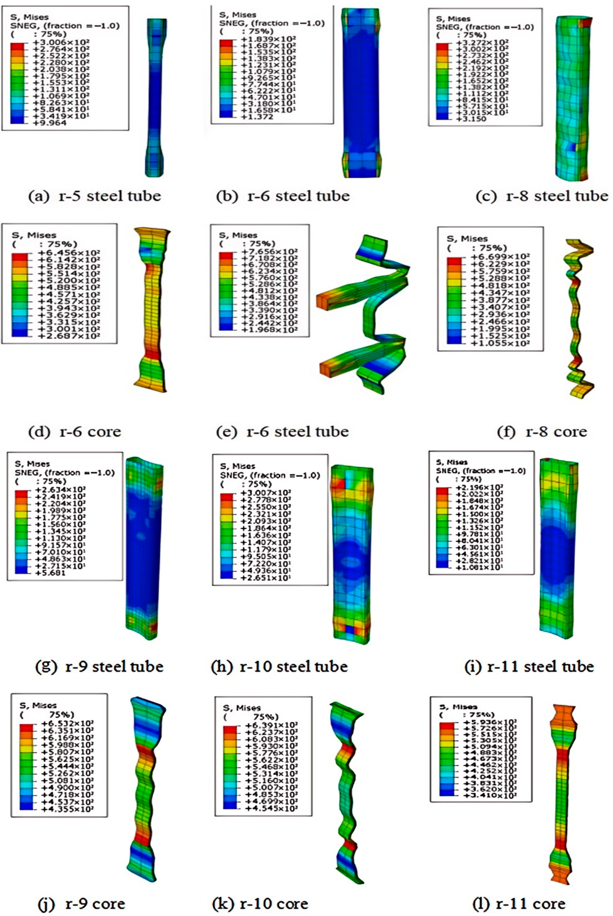
Finite element simulations indicated generally stable hysteretic responses in most buckling-restrained braces, with stress contours under peak axial load showing no failure signs, confirming effective core restraint. Six models (r-5, r-7, r-10, r-11, r-12, and r-13), however, displayed localized buckling failure, as illustrated in Figure 11.

In all six models exhibiting local buckling, the highest stress levels are consistently found at the transition regions where the corrugation geometry changes most abruptly—typically at the junctions between the flat segments and the curved corners of the corrugated profile. This phenomenon is particularly pronounced on the outer surface of the steel tube, where geometric discontinuities create natural stress raisers. Notably, the stress concentration is not confined to a single axis; rather, it manifests prominently on both the strong axis and the weak axis, indicating a complex three-dimensional stress state that engages the entire cross-section. On the weak axis, the stress concentration arises from the combined effects of axial compression and bending induced by the corrugated geometry. On the strong axis, the concentration stems from the confinement pressure exerted by the core concrete as it expands laterally under compression, which forces the steel tube to resist hoop stresses.

To facilitate observation, the deformation of the six buckling-restrained supports exhibiting localized failure was magnified. The characteristic feature of this localized failure is the pronounced bulging of the restraining elements (Figure 12). To investigate the stress distribution within each component of the buckling-restrained support in greater detail, the core and restraining elements were isolated from the composite structure, and their stress distribution plots were examined (Figure 12). The buckling modes of the core unit’s steel supports clearly reveal their divergence from the overall buckling behavior of the buckling-restrained support. The steel supports in the core unit exhibit localized bulging deformations, leading to uneven stress distribution within the support. This causes stresses to concentrate in areas of greater deformation, thereby affecting the hysteretic behavior of the buckling-restrained support.

Based on the results of isolating the core and restraint units from the overall structure and examining their stress contour plots, for the straight-line support configuration, the stress distribution within the corrugated steel pipe of the restraint unit exhibits a pronounced change as the external axial compressive load increases. As the external axial compressive load increases, the core unit of the steel support undergoes buckling and makes contact with the restraint unit. At this point, the restraint unit begins to bear the load. The local buckling half-wave number of the core unit steel support continuously increases, while its wavelength progressively decreases. Chen [3] believes that it leads to a constant increase in the local squeezing force between the core unit steel support and the restraint unit. Due to the relatively low tensile bearing capacity of concrete, the concrete on the weak axis of the support cracks under tension shortly after contact. At this point, Chen [3] claims that the elliptical steel tube on the weak axis bears tensile stress. Ultimately, this exceeds the resistance capacity of the confinement unit, rendering it incapable of providing effective confinement. Considering the stress distribution, the locations where the outer casing bulges are nearly all points of stress concentration on the weak axis. This subsequently causes the buckling-confinement support to undergo localized instability failure.

Although Takeuchi et al. previously conducted similar research, their work was based on conventional cross-sections, employed either an elastic–perfectly plastic or bilinear steel model, and utilized unbonded layers or gaps to achieve restraint [22]—differing slightly from the design approach adopted in this study. However, both investigations concur that insufficient restraint stiffness is the fundamental cause of local bulging, and both observed that bulging occurs in the stress-concentration zone along the weak axis. Specifically, in the present study, models with a wall thickness of 12 mm or more (e.g., r-3 and r-4) did not experience bulging, whereas models with a thickness of only 2 mm generally bulged when the angle exceeded 45°. This directly corroborates Takeuchi’s key conclusion: restraint stiffness is the primary factor in preventing bulging [22]. Furthermore, reducing the corner radius from 45 mm to 40 mm in this study induced bulging, which aligns with Takeuchi’s assertion that geometric discontinuities in the restrainer are prone to triggering local buckling [22].

To align the numerical results of this study with practical engineering guidelines, reference was made to the performance acceptance criteria recommended in NIST GCR 10-917-5, Seismic Design of Buckling-Restrained Braced Frames. First, the loading protocol employed in this study covers core strains ranging from 0.94% to 3.44%, satisfying the anticipated strain demands for design-level earthquakes specified in the brief [23]. Second, the hysteresis curves of all non-bulging models are full and exhibit no significant pinching; their calculated equivalent viscous damping ratios exceed the NIST-recommended threshold of 0.25 [23], thereby demonstrating excellent energy-dissipation capacity.

Taking the cycle at a displacement amplitude of 22 mm for Model e-5 as an example, the calculation of the equivalent viscous damping ratio ζeq is illustrated. This cycle corresponds approximately to the time interval from t = 1.0 to t = 2.0. From the ALLPD history, the increment of cumulative plastic dissipation energy over this cycle is obtained as Ediss = 4.60 × 10⁸ N·mm. From the hysteresis curve, the maximum load (average of absolute tensile and compressive peaks) is Fmax = 8.5 × 10⁶  N at a displacement amplitude of δ_max = 22 mm. The elastic strain energy is

$$E_{el}={\displaystyle \frac{1}{2}}{F}_{\max }\cdot {\delta }_{\max }=9.35\times {10}^7 \mathrm{N}\cdot \mathrm{mm}$$

Substituting into the formula:

$${\xi }_{eq}={\displaystyle \frac{1}{2\pi }}\cdot {\displaystyle \frac{E_{diss}}{E_{el}}}=0.78$$

Additionally, the displacement amplitude of 44 mm, the Ediss = 4.97 × 10⁸ N·mm. From the hysteresis curve, the Fmax = 10.0 × 10⁶ N at a displacement amplitude of δ_max = 44 mm. The elastic strain energy is

$$E_{el}={\displaystyle \frac{1}{2}}{F}_{\max }\cdot {\delta }_{\max }=2.2\times {10}^8 \mathrm{N}\cdot \mathrm{mm}$$

Substituting into the formula:

$${\xi }_{eq}={\displaystyle \frac{1}{2\pi }}\cdot {\displaystyle \frac{E_{diss}}{E_{el}}}=0.36$$

Moreover, the compression-strength adjustment factor β remains below 1.3 at each loading stage, and its average value also satisfies the limit of 1.15, further confirming the rationality of the model design.

Taking Model i-1 as an example, its loading protocol consists of three displacement amplitudes (15 mm, 39 mm, and 55 mm), with one cycle performed at each amplitude. The peak loads for each cycle are extracted from the hysteresis curve data, where the tensile load is taken as the positive maximum and the compressive load as the negative minimum (i.e., maximum absolute value). The compression strength adjustment factor β is calculated using the following formula:

$$\beta ={\displaystyle \frac{P_{\max ,comp}}{P_{\max ,tens}}}$$

where P_max,comp is the maximum compressive load (taken as absolute value), and P_max,tens is the maximum tensile load. The calculated results are presented in

Table 14. β values of Model i-1 for each loading cycle.

Cycle No.	Displacement Amplitude (mm)	Pmax,comp (kN)	Pmax,tens (kN)	β
1	15	9734	5376	1.81
2	39	10,010	8482	1.18
3	55	10,211	9313	1.10

.

As shown in the table, except for the first cycle, where the β value is slightly above 1.3, all subsequent cycles satisfy the β ≤ 1.3 requirement [12]. Considering the potential degree of discreteness in practical engineering and the general practice of adopting the maximum tensile–compressive strength ratio within the structure as the standard [24], the model’s overall compressive stability remains within an acceptable range.

2.3.3. Comparative Analysis

From a structural performance perspective, when comparing single-parameter data, elliptical sleeves exhibit significantly higher load-bearing capacity than rectangular and corrugated sleeves at equivalent wall thicknesses. However, rectangular steel tubes (i-1) and corrugated steel tubes (r-3) demonstrate remarkably similar stress values at Py under identical wall thicknesses (rectangular tubes being approximately 0.6% higher), with neither exhibiting buckling instability. Elliptical steel tubes, conversely, are prone to buckling compared to the other two types. Overall, the three types exhibit nearly equivalent performance in terms of static yield load-bearing capacity and resistance to buckling instability.

Furthermore, considering the research in this chapter on parameters affecting load-bearing capacity, although non-rectangular casings may buckle under specific conditions, optimizing geometric parameters such as wall thickness or corrugation corner radius can further improve stress distribution and enhance load-bearing efficiency, thereby achieving higher material utilization.

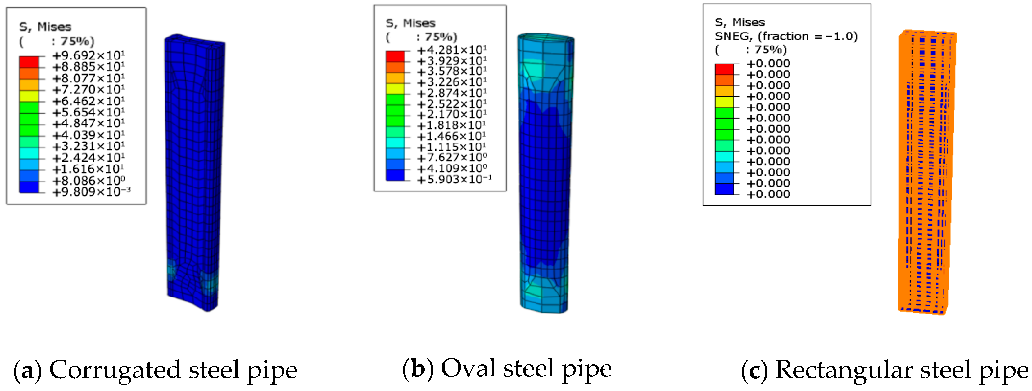
From a material-saving perspective, non-rectangular outer casings, such as elliptical or corrugated designs, demonstrate superior material utilization efficiency compared to rectangular counterparts. The key distinction lies in the fact that when interactions along the minor axis are eliminated (Figure 13), the concrete and outer casing within rectangular systems bear negligible loads (Figure 14), indicating their material strength remains largely untapped. whereas non-rectangular casings maintain a certain stress distribution under identical conditions (Figure 14), demonstrating a higher material contribution rate. This fact illustrates that the geometric characteristics of non-rectangular cross-sections enable more efficient load transfer and distribution. Consequently, they may reduce material usage while achieving equivalent confinement effects, or provide higher load-bearing capacity with the same material input, thereby delivering superior economic benefits.

To quantitatively assess the efficiency of steel utilization for different cross-sectional shapes, a material efficiency index η is defined as:

$$\eta ={\displaystyle \frac{P_y}{{\sigma }_y\cdot A_{steel}}}$$

where Py is the ultimate axial load of the BRB (N), σ_y is the yield strength of steel (taken as 235 MPa for Q235 steel), and Asteel is the total cross-sectional area of steel per unit length of the BRB (mm²), comprising both the core steel and the outer steel tube. The core steel has dimensions of 160 mm × 25 mm, giving a cross-sectional area Acore = 4000 mm². The cross-sectional area of the outer casing, Acasing, is calculated according to the specific geometry of each section.

Based on this definition,

Table 15. Elliptical steel tubes comparable to rectangular steel tubes.

Number	w (°)	d (mm)	t (mm)	Py (N)	Local Bulging Observed	β
r-3	45	45	12	8,049,170	No	1.30
e-6			12	9,428,560	Yes	1.21
i-1			12	8,098,140	No	1.10

summarizes the material efficiency indices for the three cross-sectional types with a wall thickness of t = 12 mm. The results (

Table 16. Material utilization efficiency index.

Number	Py (N)	Acasing (mm2)	Asteel (mm2)	η
r-3	8,049,170	No	1.04	1.93
e-6	9,428,560	Yes	1.07	2.70
i-1	8,098,140	No	1.06	2.04

) show that the elliptical section achieves the highest η value of 2.70, which is approximately 40% higher than that of the rectangular section (η = 1.93); the corrugated section yields an η of 2.04, about 6% higher than the rectangular counterpart. These findings indicate that, for the same amount of steel, non-rectangular sections—especially the elliptical shape—can more effectively exploit the material’s load-bearing capacity, offering significant material economy.

3. Results

This study systematically investigated the seismic performance of non-rectangular concrete-filled steel tube buckling-restrained braces through comprehensive finite element simulations, with particular focus on elliptical and corrugated cross-sections and the influence of key geometric parameters, including wall thickness, corner radius, and corrugation angle.

The results demonstrate that optimized non-rectangular configurations can achieve load-bearing capacity comparable to conventional rectangular designs while significantly improving material efficiency, particularly along the weak axis. For elliptical sections, load-bearing capacity increases consistently with wall thickness, accompanied by stable hysteretic behavior, confirming the advantages of smooth curvature in distributing stresses uniformly and utilizing additional material effectively. For corrugated sections, a critical thickness threshold was identified: below this threshold, thin walls leverage geometric flexibility to achieve superior energy dissipation; beyond it, further capacity gains diminish rapidly, and hysteresis loops become progressively pinched, revealing an inherent trade-off between strength and energy dissipation in corrugated geometries. The influence of corner radius exhibits a non-monotonic pattern: an optimal radius achieves a balance between capacity and full, stable hysteresis; smaller radii, while triggering local buckling, temporarily enhance capacity; larger radii yield higher peak loads but at the cost of irregular hysteretic response. Corrugation angle similarly demonstrates complex behavior: moderate angles provide reliable energy dissipation; a specific angle emerges as an optimal section, balancing high strength with fine hysteretic quality; excessive angles, despite promoting distributed buckling modes that improve loop fullness, cannot compensate for the accompanying reduction in capacity. Failure analysis consistently identified local buckling initiation at geometrically discontinuous transition regions, where significant stress concentrations develop on both strong and weak axes, underscoring the critical role of geometric continuity in ensuring stability.

Comparative analysis reveals that at equivalent wall thickness, elliptical sections achieve the highest absolute capacity but with buckling susceptibility, while rectangular and corrugated sections maintain stable response, with non-rectangular geometries demonstrating superior material utilization through more uniform cross-sectional stress transmission. All stable models satisfy relevant seismic design code requirements for strength adjustment and exceed prescribed energy dissipation thresholds, confirming their viability for seismic applications.

Building upon the insights gained from this study and acknowledging its inherent limitations, future research can be pursued in the following directions:

First, experimental validation is essential to bridge the gap between numerical simulation and engineering practice. As this study relies exclusively on finite element analysis, the conclusions drawn require verification through full-scale or scaled model testing. Priority should be given to quasi-static cyclic tests on the optimized configurations identified herein—such as elliptical sections with moderate wall thickness, corrugated sections near the critical thickness threshold, and those with 45 mm corner radius or 60° corrugation angle—to systematically examine failure modes, hysteretic performance, and energy dissipation capacity, thereby calibrating numerical models and establishing reliable design parameters.

Second, the analysis should be extended to more realistic seismic conditions. This study considered only static and quasi-static cyclic loading, without accounting for dynamic effects, spectral characteristics, cumulative damage or multi-directional excitation inherent in real earthquake ground motions. Subsequent research should employ dynamic time-history analyses using real ground motion records to capture the response of non-rectangular BRBs under velocity, acceleration, and higher-mode effects. Multi-component seismic inputs and soil-structure interaction should also be incorporated to provide a comprehensive assessment of performance under actual service conditions.

Third, simplified design methods and empirical formulas should be developed for practical engineering use. This study has revealed intrinsic relationships between key geometric parameters—wall thickness, corner radius, and corrugation angle—and structural performance indicators such as load-bearing capacity and hysteretic behavior. Based on the parametric results, regression analyses could yield simplified equations that enable engineers to quickly estimate critical performance metrics. In parallel, construction detailing recommendations and design guidelines should be formulated for each cross-section type to facilitate the adoption of non-rectangular BRBs in practice.

Fourth, the observed sensitivity of buckling occurrence to the loading protocol (e.g., the comparison between Models e-5 and e-6) underscores the necessity of considering realistic seismic loading histories in design. Future research should investigate the cumulative damage and low-cycle fatigue behavior under various loading protocols to establish more robust design criteria.

4. Conclusions

This study systematically evaluated the seismic performance of elliptical and corrugated concrete-filled steel tube buckling-restrained braces through finite element simulations, with emphasis on the influence of key geometric parameters, including wall thickness, corner radius, and corrugation angle. The main conclusions are as follows:

• Elliptical sections exhibit monotonic improvement in load-bearing capacity with increasing wall thickness (a 75% increase from 1 mm to 12 mm) and stable hysteretic behavior, attributed to uniform stress distribution enabled by their smooth curvature. However, compared to rectangular sections, they are more susceptible to local buckling under severe cyclic loading.
• Corrugated sections display a critical thickness threshold of approximately 10 mm: below this threshold, thin walls leverage geometric flexibility to achieve superior energy dissipation and full hysteresis loops; beyond it, capacity gains become marginal and hysteresis loops exhibit progressive pinching, revealing an inherent trade-off between strength and energy dissipation.
• Both corner radius and corrugation angle influence performance non-monotonically. An optimal combination balances load-bearing capacity with stable, full hysteresis. Deviations from these values trigger local buckling and irregular response, while a 60° angle achieves high strength while maintaining good hysteretic quality, representing a design “sweet spot.”
• Non-rectangular shapes significantly improve material utilization efficiency. At equivalent steel consumption, elliptical sections achieve an efficiency index 40% higher than rectangular sections, and corrugated sections 6% higher, demonstrating that shape optimization can reduce material consumption while maintaining or enhancing structural performance.

These findings provide quantitative guidance for optimizing non-rectangular BRB geometries, enabling engineers to balance load-bearing capacity, energy dissipation, and material economy according to specific performance objectives.

References

1. Abdewi, E.F.; Sulaiman, S.; Hamouda, A.M.S.; Mahdi, E. Quasi-static axial and lateral crushing of radial corrugated composite tubes. Thin-Walled Struct. 2008, 46, 320–332. [Google Scholar] [CrossRef] [Scilit]
2. Loughlan, J.; Yidris, N. The failure of thin-walled lipped channel compression members due to coupled local-distortional interactions and material yielding. Thin-Walled Struct. 2012, 61, 14–21. [Google Scholar] [CrossRef] [Scilit]
3. Chen, H. Research on the Hysteretic Behavior of Corrugated Steel Tube Concrete Buckling-Restrained Braces. Master’s Thesis, Harbin Institute of Technology, Harbin, China, 2021. [Google Scholar]
4. Sheng, M. Research on the Composite Load-Bearing Performance and Design Method of Elliptical Steel Tube Concrete Members. Master’s Thesis, Hefei University of Technology, Hefei, China, 2020. [Google Scholar]
5. Zhou, Y.; Shao, H.; Lui, E.M.; Zhong, G.; Li, Z. Behavior of elliptical buckling-restrained braces under cyclic axial load. Structures 2023, 48, 331–345. [Google Scholar] [CrossRef] [Scilit]
6. He, K.; Yuan, H.; Zhao, Y.; Du, X. External load crushing strength of corrugated steel-reinforced concrete pipes: Experimental testing and numerical study. Eng. Struct. 2024, 292, 112388. [Google Scholar] [CrossRef] [Scilit]
7. Li, H.; Du, Y.; Han, J.; Li, F.; Chi, P. Experimental and numerical study of low-yield-point steel corrugated pipe dampers. Soil Dyn. Earthq. Eng. 2024, 180, 108615. [Google Scholar] [CrossRef] [Scilit]
8. Liu, Z.; Shu, G.; Yao, Z.; Bian, Z.; Yun, Z.; Cheng, H.; Mao, D. Study on the Axial Compression Mechanical Performance of Double-Skin Composite Tubular Column with Inner Corrugated Steel Pipe Short Columns. J. Southwest Jiaotong Univ. 2026. Available online: https://link.cnki.net/urlid/51.1277.U.20260126.1314.002 (accessed on 3 January 2026).
9. Lin, P.C.; Tsai, K.C.; Chang, C.A.; Hsiao, Y.Y.; Wu, A.C. Seismic design and testing of buckling-restrained braces with a thin profile. Earthq. Eng. Struct. Dyn. 2016, 45, 339–358. [Google Scholar] [CrossRef] [Scilit]
10. Feklistova, E.V.; Mugatarov, A.I.; Wildemann, V.E.; Agishev, A.A. Fracture processes numerical modeling of elastic-brittle bodies with statistically distributed subregions strength values. Frat. Integrità Strutt. 2024, 68, 325–339. [Google Scholar] [CrossRef] [Scilit]
11. Wei, X.; Wu, C.T.; Xiao, L.; Li, J. Hot spot stress analysis of CFST joints considering steel–concrete contact characteristics. Adv. Eng. Sci. 2021, 53, 62–67. [Google Scholar] [CrossRef]
12. American Institute of Steel Construction. Seismic Provisions for Structural Steel Buildings; American Institute of Steel Construction: Chicago, IL, USA, 2010. [Google Scholar]
13. Shu, K. Study on the Performance of Double Steel Tube Buckling-Restrained Brace with Built-In Stiffeners. Master’s Thesis, Zhejiang University, Hangzhou, China, 2018. [Google Scholar]
14. Shi, Y.; Wang, M.; Wang, Y. Experimental study on constitutive relation of structural steel under cyclic loading. J. Build. Mater. 2012, 15, 293–300. [Google Scholar]
15. Popovics, S. A numerical approach to the complete stress-strain curve of concrete. Cem. Concr. Res. 1973, 3, 583–599. [Google Scholar] [CrossRef] [Scilit]
16. Wang, Y.; Yang, L.; Yang, H.; Liu, C. Behavior of concrete-filled corrugated steel tubes under axial compression. Eng. Struct. 2019, 183, 110887. [Google Scholar] [CrossRef] [Scilit]
17. Yang, L.; Wang, Y.; Elchalakani, M.; Fang, Y. Experimental behavior of concrete-filled corrugated steel tubular short columns under eccentric compression and non-uniform confinement. Eng. Struct. 2020, 220, 110998. [Google Scholar] [CrossRef] [Scilit]
18. Fang, Y.; Liu, C.; Yang, H.; Yang, L. Axial behavior of concrete-filled corrugated steel tubular column embeded with structural steel. J. Constr. Steel Res. 2020, 170, 106108. [Google Scholar] [CrossRef] [Scilit]
19. Fang, Y.; Wang, Y.Y.; Hou, C.; Lu, B. CFDST stub columns with galvanized corrugated steel tubes: Concept and axial behavior. Thin-Walled Struct. 2020, 157, 107073. [Google Scholar] [CrossRef] [Scilit]
20. Murthy, A.R.; Palani, G.S.; Iyer, N.R. State-of-the-art review on fracture analysis of concrete structural components. Sādhanā 2009, 34, 345–367. [Google Scholar] [CrossRef] [Scilit]
21. Zeng, C.; Zhang, Y.; Zhao, J.; Xu, G.; Wang, D.; Pan, T. A partially buckling-restrained brace with T-shaped double core for seismic retrofit: Experimental study, numerical analysis, and local stability design. Eng. Struct. 2023, 276, 115378. [Google Scholar] [CrossRef] [Scilit]
22. Takeuchi, T.; Hajjar, J.F.; Matsui, R.; Nishimoto, K.; Aiken, I. Local buckling restraint condition for core plates in buckling restrained braces. J. Constr. Steel Res. 2010, 66, 139–149. [Google Scholar] [CrossRef] [Scilit]
23. NIST GCR 10-917-5; Nonlinear Structural Analysis for Seismic Design (NEHRP Seismic Design Technical Brief No. 4, NIST GCR 10-917-5). National Institute of Standards and Technology: Gaithersburg, MD, USA, 2010. Available online: https://www.nehrp.gov/pdf/nistgcr10-917-5.pdf (accessed on 26 February 2026).
24. Tsai, K.C.; Wu, A.C.; Wei, C.Y.; Lin, P.C.; Chuang, M.C.; Yu, Y.J. Welded end-slot connection and debonding layers for buckling-restrained braces. Earthq. Eng. Struct. Dyn. 2014, 43, 1785–1807. [Google Scholar] [CrossRef] [Scilit]
Figure 1. Concrete-constrained buckling-restrained brace for non-circular steel tube.
Buildings 16 01228 g001
Figure 2. Finite element mesh generation for corrugated steel tubes.
Buildings 16 01228 g002
Figure 3. High-contrast warning for the grid division of the Model e-5 steel tubes. (Yellow highlights indicate errors).
Buildings 16 01228 g003
Figure 4. First diagram of the Model e-5’s drumming position.
Buildings 16 01228 g004
Figure 5. Cross-section and geometric parameters display.
Buildings 16 01228 g005
Figure 6. Hysteresis curve comparison.
Buildings 16 01228 g006
Figure 7. The corresponding hysteresis curve.
Buildings 16 01228 g007
Figure 8. The corresponding hysteresis curves.
Buildings 16 01228 g008
Figure 9. The corresponding hysteresis curves.
Buildings 16 01228 g009
Figure 10. The corresponding hysteresis curves.
Buildings 16 01228 g010
Figure 11. Stress contour maps of buckling-restrained supports exhibiting localized buckling failure.
Buildings 16 01228 g011
Figure 12. Longitudinal cross-section under load.
Buildings 16 01228 g012
Figure 13. Interaction contact surface configuration.
Buildings 16 01228 g013
Figure 14. Stress conditions of the casing and concrete.
Buildings 16 01228 g014