Simulation of Nonstationary Fluctuating Wind Fields Using POD Decoupling and Spline Interpolation

Abstract

Improving the simulation efficiency of the spectral representation method (SRM) for nonstationary fluctuating wind fields has attracted considerable attention. To this end, this study proposes a method based on proper orthogonal decomposition (POD) decoupling and Spline interpolation to enhance computational efficiency. This method selects a limited number of interpolation points in the time-frequency domain of the evolutionary power spectral density (EPSD) for Cholesky decomposition, utilizes the proper orthogonal decomposition (POD) technique to achieve time-frequency decoupling of the spectral matrix, and employs Spline interpolation but not the traditional Hermite-interpolation to reconstruct the complete time-frequency functions, thereby enabling the rapid synthesis of wind-velocity time histories via the FFT. Then, the wind field on a three-span frame lightning-rod structure is taken as an example to validate the reliability of the proposed method. The influences of the modal order and the number of time-frequency interpolation points on both simulation efficiency and error are investigated, and comparisons are given with the Hermite-interpolation-based method. The results indicate that the simulation efficiency is governed primarily by the modal order, and the method with Spline interpolation shows higher computational efficiency and accuracy because it can satisfy accuracy requirements at a lower modal order. Finally, a rational truncation criterion based on the cumulative energy ratio of at least 99.9% is suggested to determine the optimal modal order, thereby achieving a balance between accuracy and computational efficiency.

1. Introduction

For a stationary wind field under a well-behaved wind environment, wind-velocity statistics such as the mean, variance, power spectral density (PSD) and coherence function are time-invariant [1,2]. However, extensive studies and field measurements have demonstrated that, in peculiar wind environments such as typhoons [3,4], downbursts [5,6], and mountainous canyon winds [7,8], the above statistics and the coherence function exhibit pronounced time-varying characteristics. In other words, the wind velocity should be modeled as a nonstationary stochastic process, and the spectrum should be described in terms of the evolutionary power spectral density (EPSD) rather than the conventional PSD.

In engineering practice, the spectral representation method or harmonic synthesis method is commonly adopted, together with empirical wind spectra and coherence functions, to generate stationary or nonstationary wind fields and to further evaluate structural wind-load effects [9,10,11,12]. The simulation of stationary wind fields has been well developed. For nonstationary wind fields, however, the simulation process is extremely time-consuming compared with the stationary case [13] because the EPSD is a coupled function of time and frequency. To improve the efficiency of nonstationary wind-field simulation, research has mainly advanced along the following two aspects [14] in the past decade.

First, interpolation is used to reduce the number of Cholesky decompositions of the EPSD. This is an effective and generally applicable approach and its application has extended from frequency interpolation for stationary wind fields to time-frequency interpolation for nonstationary wind fields [15,16,17,18,19,20,21]. The decomposed spectral matrix (hereafter referred to as the H matrix) could be reconstructed using time-frequency interpolation functions.

Second, the H matrix is decoupled in the time-frequency domain to enable FFT-accelerated harmonic superposition. Using FFT techniques to perform harmonic superposition for stationary wind-field simulation has become a mature and efficient scheme [22,23]. However, since the EPSD of a nonstationary wind field is a function of both time and frequency, FFT cannot be directly invoked. To address this issue, various techniques have been proposed, such as the orthogonal polynomial method [24], wavelet-based spectral superposition [25], proper orthogonal decomposition (POD) [26], non-negative matrix factorization (NMF) [27,28], and as well other approaches [29]. These methods decouple the time-frequency coupled H matrix into a sum of products of independent time functions and frequency functions, thereby allowing the FFT to be reintroduced for the frequency-dependent functions.

In addition, by combining the above two stages, some studies have further performed time-frequency decoupling of the H matrix and the interpolation-based reconstruction of the time and frequency functions after the interpolation-enhanced Cholesky decomposition [29,30]. In this case, the selections of the decoupling scheme and the interpolation function jointly determine the simulation accuracy and efficiency. For large-scale wind-field simulation, it is necessary to investigate the influences of the decoupling scheme and the interpolation function on both the accuracy and efficiency.

Based on a detailed review of existing fast simulation methods for nonstationary wind fields, this study proposes a nonstationary wind-field simulation method based on POD-based decoupling and Spline interpolation. Specifically, a limited number of interpolation points are first selected in both the time and frequency directions for the EPSD, at which Cholesky decompositions are performed. The resulting H matrix is then decoupled via POD to obtain independent time functions and frequency functions. Next, Spline interpolation is employed to reconstruct the full time-frequency functions, thereby enabling FFT-based harmonic superposition for wind-field simulation. Finally, numerical examples and comparisons with existing methods are presented to validate the correctness of the proposed method and to demonstrate its superior computational efficiency.

2. Theoretical Background

In the simulation of a fluctuating wind field, the spatially continuous wind field should be discretized into multiple simulation points and represented as an m-dimensional zero-mean stochastic process X(t) = [x₁(t), x₂(t), …, x_m(t)]^T, where x_i(t) denotes the fluctuating wind-velocity time history at the ith point (i = 1, 2, …, m), and m is the number of simulation points. For a nonstationary wind field, the cross-correlation function matrix of X(t) and the corresponding EPSD can be expressed by Equations (1) and (2), respectively:

$$R(t, t+\mathsf{\tau })=\left[\begin{array}{cccc}{R}_{11}(t, t+\mathsf{\tau })& R_{12}(t, t+\mathsf{\tau })& \dots & R_{1m}(t, t+\mathsf{\tau })\\ R_{21}(t, t+\mathsf{\tau })& R_{22}(t, t+\mathsf{\tau })& \dots & R_{2m}(t, t+\mathsf{\tau })\\ ⋮& ⋮& \ddots & ⋮\\ R_{m1}(t, t+\mathsf{\tau })& R_{m2}(t, t+\mathsf{\tau })& \dots & R_{\mathit{mm}}(t, t+\mathsf{\tau })\end{array}\right]$$

(1)

$$S(\omega , t)=\left[\begin{array}{cccc}{S}_{11}(\omega , t)& S_{12}(\omega , t)& \dots & S_{1m}(\omega , t)\\ S_{21}(\omega , t)& S_{22}(\omega , t)& \dots & S_{2m}(\omega , t)\\ ⋮& ⋮& \ddots & ⋮\\ S_{m1}(\omega , t)& S_{m2}(\omega , t)& \dots & S_{\mathit{mm}}(\omega , t)\end{array}\right]$$

(2)

where t is the time variable, τ is the time lag, and R_jk(t, t + τ) denotes the auto-/cross-correlation function between x_j(t) and x_k(t); ω is the circular frequency (rad/s); and S_jk(ω, t) denotes the auto-/cross-evolutionary power spectral density function between the jth and kth components, which can be evaluated by the following equation:

$$S_{\mathit{jk}}(\omega , t)=\sqrt{S_{\mathit{jj}}(\omega , t)S_{\mathit{kk}}(\omega , t)}{\mathsf{\gamma }}_{\mathit{jk}}(\omega , t)$$

(3)

where γ_jk(ω, t) is the spatial coherence function. It should be noted that S_jj(ω, t) and S_kk(ω, t) are the auto-EPSDs which are determined by specific empirical spectral models (e.g., the Kaimal spectrum used in Section 4.1, given by Equations (30)–(32)). Equation (3) is essentially used to determine the off-diagonal terms in the EPSD matrix. A commonly adopted form is the Davenport coherence function, as given in Equations (4):

$${\mathsf{\gamma }}_{\mathit{jk}}(\omega , t)=\exp \left\{{\displaystyle \frac{-\omega {[C_x^2{(x_j-x_k)}^2+C_y^2{(y_j-y_k)}^2+C_z^2{(z_j-z_k)}^2]}^{1/2}}{\mathsf{\pi }(\tilde{U}(z_j, t)+ \tilde{U}(z_k, t))}}\right\}$$

(4)

where a Cartesian coordinate system is adopted in which the x, y, and z axes represent the longitudinal (along-wind), lateral (across-wind), and vertical directions, respectively. Accordingly, C_x = 6, C_y = 16, and C_z = 10 are the longitudinal, lateral, and vertical decay coefficients, respectively [31]; and $\tilde{U}(z_j, t)$ and $\tilde{U}(z_k, t)$ denote the instantaneous mean wind velocities at points j and k at time t, respectively.

The EPSD in Equation (2) can be subjected to the Cholesky decomposition as

$$S(\omega , t)=H(\omega , t)H^{T*}(\omega , t)$$

(5)

$$H(\omega , t)=\left[\begin{array}{cccc}{H}_{11}(\omega , t)& 0& \dots & 0\\ H_{21}(\omega , t)& H_{22}(\omega , t)& \dots & 0\\ ⋮& ⋮& \ddots & ⋮\\ H_{m1}(\omega , t)& H_{m2}(\omega , t)& \dots & H_{\mathit{mm}}(\omega , t)\end{array}\right]$$

(6)

where H(ω, t) is a lower triangular matrix, and H^T*(ω, t) denotes the complex conjugate transpose of H(ω, t). Its element H_jk(ω, t) can be written in the polar form as

$$H_{\mathit{jk}}(\omega , t)=|H_{\mathit{jk}}(\omega , t)|e^{i{\theta }_{\mathit{jk}}(\omega , t)}$$

(7)

$${\theta }_{\mathit{jk}}(\omega , t)={\tan }^{-1}({\displaystyle \frac{\mathrm{Im}[H_{\mathit{jk}}(\omega , t)]}{\mathrm{Re}[H_{\mathit{jk}}(\omega , t)]}})$$

(8)

where |·| denotes the modulus of a complex number; θ_jk(ω, t) is the phase angle of H_jk(ω, t); and Im[·] and Re[·] represent the imaginary and real parts of a complex number, respectively.

Accordingly, the fluctuating wind-velocity time history x_j(t) at an arbitrary simulation point j can be obtained by harmonic superposition as follows:

$$\begin{array}{cc}\hfill x_j(t)& =2\sqrt{\Delta \omega }{\displaystyle \sum _{k=1}^j{\displaystyle \sum _{l=1}^N|}} H_{\mathit{jk}}({\omega }_l, t)|\cos [{\omega }_{l}t-{\theta }_{\mathit{jk}}({\omega }_l, t)+{\mathsf{\phi }}_{\mathit{kl}}]\hfill \\ & =2\sqrt{\Delta \omega }\mathrm{Re}\left\{{\displaystyle \sum _{k=1}^j{\displaystyle \sum _{l=1}^N{H}_{\mathit{jk}}}}({\omega }_l, t)e^{i({\omega }_{l}t+{\mathsf{\phi }}_{\mathit{kl}})}\right\}\hfill \end{array}$$

(9)

where Δω = ω_u/N is the frequency increment, with ω_u being the cut-off frequency and N the number of frequency components; ω_l = lΔω (l = 1, 2, …, N) denotes the single-index angular frequency. Since a nonstationary process does not satisfy ergodicity, the single-index frequency discretization is adopted [32]. In addition, φ_kl is a set of independent random phase angles, which are uniformly distributed over [0, 2π].

For the cut-off frequency ω_u, it should be determined according to two critical factors: the energy distribution of the target wind spectrum and the dynamic characteristics of the structure. On one hand, since the energy of natural wind is predominantly concentrated in the low-frequency range (generally below 0.5 Hz), the selected cut-off frequency must be sufficiently high to capture the majority of the fluctuation energy in the evolutionary power spectral density (EPSD) [33]. On the other hand, it is crucial to ensure that ω_u covers the dominant natural frequencies of the target structure to correctly excite the resonant responses [13].

It should be noted that the above formulation is established for nonstationary stochastic processes. If the nonstationary and time-varying characteristics of the wind field are neglected, Equations (1)–(8) degenerate into a time-invariant stationary stochastic process, and the time-varying mean wind speed further reduces to a constant mean wind speed.

3. Nonstationary Wind-Field Simulation Based on POD Decoupling and Spline Interpolation

3.1. Selection of Interpolation Points

Since the EPSD exhibits different variation characteristics along the time and frequency directions, the selection of time-frequency interpolation points prior to the Cholesky decomposition should be treated differently in the two dimensions. According to Zhao and Jiang [30], a uniform distribution is suitable in the time direction (Equation (10)), whereas a non-uniform distribution is more appropriate in the frequency direction. Moreover, the adopted quartic polynomial can be tuned to meet the required distribution of frequency points (Equation (11)), providing higher adaptability. The same strategy is adopted here for selecting the time-frequency interpolation points.

$${ \tilde{t}}_i={\displaystyle \frac{i-1}{N_t-1}}{T}_0,\hspace{0.33em}\hspace{0.33em}i=1, 2,\dots , N_t$$

(10)

$${ \tilde{\omega }}_r=({\omega }_u-{\omega }_1)({\displaystyle \frac{r-1}{N_{\omega }-1}}{)}^{4\kappa }+{\omega }_1,\hspace{0.33em}\hspace{0.33em}r=1, 2,\dots , N_{\omega }$$

(11)

where ${ \tilde{t}}_i$ and ${ \tilde{\omega }}_r$ denote the interpolation points in the time and frequency directions, respectively; T₀ is the total simulation duration; N_t and N_ω are the number of interpolation points in time and frequency, respectively, which should generally satisfy N_t << M and N_ω << N, where M and N are the total numbers of time and frequency points; ω₁ and ω_u are the lower and upper bounds of the frequency range; and κ is an adjustable parameter controlling the degree of non-uniformity.

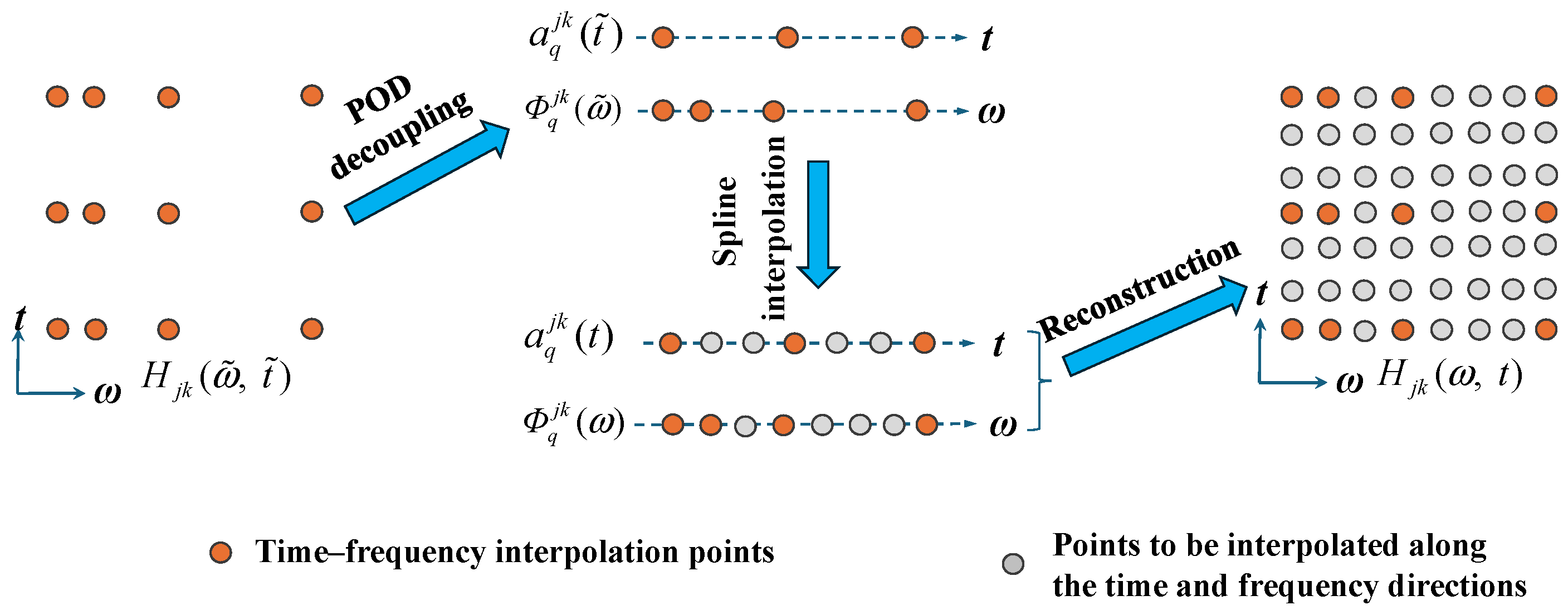
After the time and frequency interpolation points $\tilde{t}$ and $\tilde{\omega }$ are determined, the Cholesky decomposition of the EPSD is performed only at the selected interpolation points. The resulting H matrix is then decoupled via POD, and Spline interpolation is subsequently employed to reconstruct the full time and frequency functions, thereby enabling FFT-based harmonic superposition. The overall procedure is illustrated in Figure 1, and the detailed decoupling and interpolation processes are presented in Section 3.2.

3.2. POD Decoupling and Spline Interpolation

Although various decoupling methods have been proposed for the H matrix, most of them [24,25,26] can be generally expressed in the following form:

$$H_{\mathit{jk}}(\tilde{\omega }, \tilde{t})={\displaystyle \sum _{q=1}^{N_{\omega }}{a}_q^{\mathit{jk}}}(\tilde{t}){\mathsf{\Phi }}_q^{\mathit{jk}}(\tilde{\omega })\approx {\displaystyle \sum _{q=1}^{N_R}{a}_q^{\mathit{jk}}}(\tilde{t}){\mathsf{\Phi }}_q^{\mathit{jk}}(\tilde{\omega })$$

(12)

where $a_q^{\mathit{jk}}(\tilde{t})$ is the qth order time function, and ${\mathsf{\Phi }}_q^{\mathit{jk}}(\tilde{\omega })$ is the qth order frequency function; N_R is the number of retained modes in the time and frequency directions.

Tao et al. [29] compared several decoupling methods and concluded that, for the POD-based approach, an effective time-frequency decoupling can be achieved by retaining only the eigenvectors associated with relatively high eigenvalue contributions, leading to a more concise and efficient procedure. Therefore, POD is also adopted in this study.

To perform POD-based decoupling, the time-frequency function $H_{\mathit{jk}}(\tilde{\omega }, \tilde{t})$ needs to be arranged into a matrix form as

$${\tilde{H}}_{\mathit{jk}}=\left[\begin{array}{cccc}{H}_{\mathit{jk}}(\Delta \tilde{\omega }, \Delta \tilde{t})& H_{\mathit{jk}}(\Delta \tilde{\omega }, 2\Delta \tilde{t})& \dots & H_{\mathit{jk}}(\Delta \tilde{\omega }, N_t\Delta \tilde{t})\\ H_{\mathit{jk}}(2\Delta \tilde{\omega }, \Delta \tilde{t})& H_{\mathit{jk}}(2\Delta \tilde{\omega }, 2\Delta \tilde{t})& \dots & H_{\mathit{jk}}(2\Delta \tilde{\omega }, N_t\Delta \tilde{t})\\ ⋮& ⋮& \ddots & ⋮\\ H_{\mathit{jk}}(N_{\omega }\Delta \tilde{\omega }, \Delta \tilde{t})& H_{\mathit{jk}}(N_{\omega }\Delta \tilde{\omega }, 2\Delta \tilde{t})& \dots & H_{\mathit{jk}}(N_{\omega }\Delta \tilde{\omega }, N_t\Delta \tilde{t})\end{array}\right]$$

(13)

For each column vector of ${\tilde{H}}_{\mathit{jk}}$, an optimal set of orthogonal basis vectors Φ (Equation (14)) is sought such that the projection of ${\tilde{H}}_{\mathit{jk}}$ onto this basis is maximized. This set of basis vectors can be obtained by performing an eigen-decomposition of the time-averaged frequency correlation matrix R [26], as given in Equations (15) and (16):

$$\Phi =[{\Phi }_1, {\Phi }_2,\dots , {\Phi }_q{]}_{N_{\omega }\times N_{\omega }},\hspace{1em}q=1, 2,\dots , N_{\omega }$$

(14)

$$R={\displaystyle \frac{1}{N_t}}{\tilde{H}}_{\mathit{jk}}{\tilde{H}}_{\mathit{jk}}^T$$

(15)

$$R{\Phi }_q={\mathsf{\lambda }}_q{\Phi }_q$$

(16)

where λ_q is the eigenvalue associated with the qth eigenvector Φ_q. It should be noted that some studies have further modified the above decoupling procedure by performing the decomposition only for the diagonal elements of the $H_{\mathit{jk}}(\tilde{\omega }, \tilde{t})$ matrix [21,34]. Although this can improve the decomposition efficiency, the mathematical and physical meanings of the resulting frequency functions are not clearly defined. Therefore, the standard POD-based decoupling approach is still the final choice here.

According to the orthogonality of the basis vectors, Equation (17) can be obtained, where $a_q=[a_1^{\mathit{jk}}(\tilde{t}),\hspace{0.33em}{a}_2^{\mathit{jk}}(\tilde{t}),\dots ,\hspace{0.33em}{a}_q^{\mathit{jk}}(\tilde{t}){]}^T$; ${\Phi }_q=[{\mathsf{\Phi }}_1^{\mathit{jk}}(\tilde{\omega }),\hspace{0.33em}{\mathsf{\Phi }}_2^{\mathit{jk}}(\tilde{\omega }),\dots ,\hspace{0.33em}{\mathsf{\Phi }}_q^{\mathit{jk}}(\tilde{\omega })]$. Since only a subset of eigenvectors corresponds to relatively large eigenvalues, the eigenvalues are reordered in descending order, and ${\tilde{H}}_{\mathit{jk}}$ (i.e., $H_{\mathit{jk}}(\tilde{\omega }, \tilde{t})$) can be approximately reconstructed in a form similar to Equation (12), as expressed by Equation (18):

$$a_q={\Phi }_q^T{\tilde{H}}_{\mathit{jk}},\hspace{1em}q=1, 2,\dots , N_R$$

(17)

$${\tilde{H}}_{\mathit{jk}}=H_{\mathit{jk}}(\tilde{\omega }, \tilde{t})\approx {\displaystyle \sum _{q=1}^{N_R}{a}_q^{\mathit{jk}}}(\tilde{t}){\mathsf{\Phi }}_q^{\mathit{jk}}(\tilde{\omega })={\displaystyle \sum _{q=1}^{N_R}{\Phi }_q}{a}_q^T$$

(18)

After $a_q^{\mathit{jk}}(\tilde{t})$ and ${\mathsf{\Phi }}_q^{\mathit{jk}}(\tilde{\omega })$ in Equation (18) are determined, interpolation is required to reconstruct the complete time and frequency functions. The Hermite interpolation adopted by Zhao and Jiang [30] guarantees only the continuity of the first derivative. To reduce the interpolation error, a higher modal order N_R is therefore required. By contrast, Spline interpolation ensures the continuity of the second derivative and generally yields smaller errors than Hermite interpolation. Hence, Spline interpolation is selected in this study to reconstruct both the time and frequency functions. The procedure is introduced below by taking $a_q^{\mathit{jk}}(\tilde{t})$ in the time direction as an example.

Let the time-step size h_i and the principal-coordinate increment a_i be defined by Equations (19) and (20). Since, in Spline interpolation, the second derivative $S^{″}(t)$ within the interval h_i = [t_i, t_i+1] is linear, Equation (21) can be obtained. By integrating it twice and using the function values at the two endpoints of the interval, a_i and a_i+1, the piecewise polynomial expression over the interval can be derived, as given in Equation (22):

$$h_i=t_{i+1}-t_i$$

(19)

$$a_i=a_q^{\mathit{jk}}(t_i)$$

(20)

$$S^{″}(t)={\displaystyle \frac{t_{i+1}-t}{h_i}}{M}_i+{\displaystyle \frac{t-t_i}{h_i}}{M}_{i+1},\hspace{1em}\hspace{0.33em}t\in [t_i,t_{i+1}],\hspace{0.33em}\hspace{0.33em}{h}_i=t_{i+1}-t_i$$

(21)

$$\begin{array}{cc}\hfill a_q^{\mathit{jk}}(t)\approx S_i(t)& ={\displaystyle \frac{M_i{(t_{i+1}-t)}^3}{6h_i}}+{\displaystyle \frac{M_{i+1}{(t-t_i)}^3}{6h_i}}\hfill \\ & +(a_i-{\displaystyle \frac{M_i{h}_i^2}{6}}){\displaystyle \frac{t_{i+1}-t}{h_i}}+(a_{i+1}-{\displaystyle \frac{M_{i+1}{h}_i^2}{6}}){\displaystyle \frac{t-t_i}{h_i}},\hspace{0.33em}\hspace{0.33em}t\in [t_i, t_{i+1}]\hfill \end{array}$$

(22)

where t_i is the ith time interpolation point; M_i is the second-derivative value at t_i; and S_i(t) denotes the Spline polynomial constructed over the ith interval.

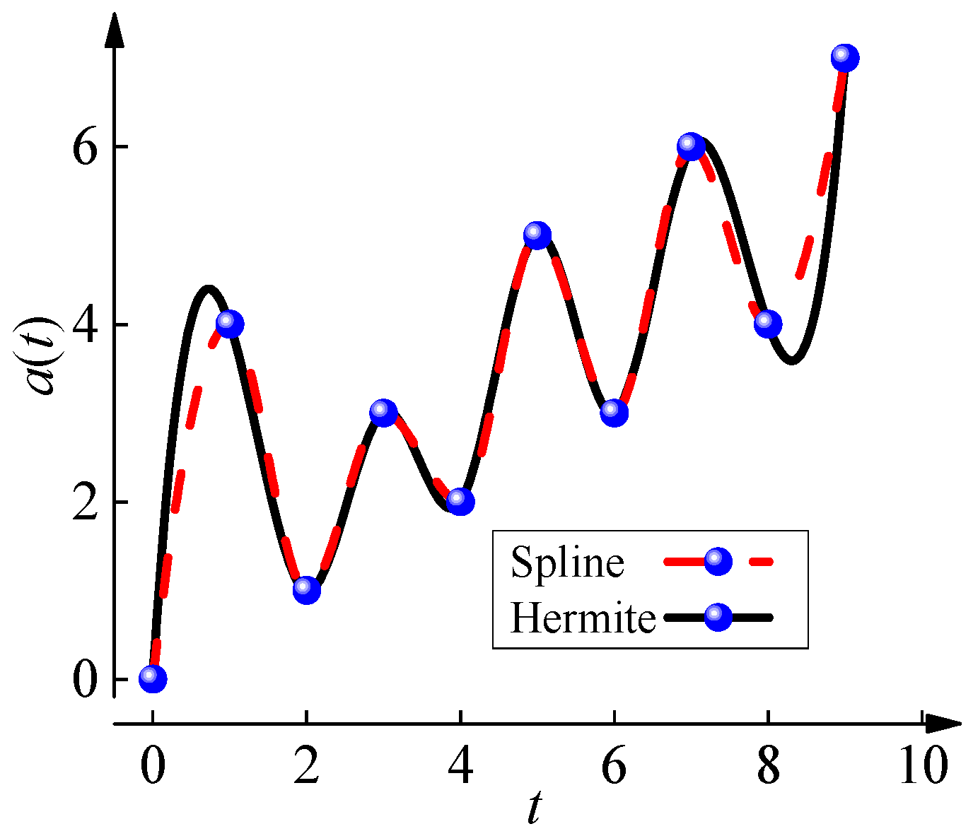
Then, taking the first derivative of Equation (22) over the intervals [t_i−1, t_i] and [t_i, t_i+1], respectively, and enforcing the equality of the left and right first derivatives at t = t_i, the system of equations governing the second derivatives at all interior nodes can be derived, as given in Equation (23). Meanwhile, according to the not-a-knot boundary condition, the continuity of the third derivative is required at the first and last interior nodes, as expressed in Equation (24). By combining Equations (23) and (24), the coefficients M_i in Equation (22) can be determined. Figure 2 presents a comparison between the piecewise functions obtained using Spline interpolation and Hermite interpolation, taking ten equally spaced time interpolation knots as an example.

$$h_{i-1}{M}_{i-1}+2(h_{i-1}+h_i)M_i+h_i{M}_{i+1}=6[{\displaystyle \frac{a_{i+1}-a_i}{h_i}}-{\displaystyle \frac{a_i-a_{i-1}}{h_{i-1}}}],\hspace{0.33em}\hspace{0.33em}i=2,\dots , N_t-1$$

(23)

$$\left\{\begin{array}{l}\begin{array}{l}{S}^{‴}(t)={\displaystyle \frac{M_{i+1}-M_i}{h_i}}\\ h_2{M}_1-(h_1+h_2)M_2+h_1{M}_3=0\end{array}\hfill \\ h_{N_t-1}{M}_{N_t-2}-(h_{N_t-2}+h_{N_t-1})M_{N_t-1}+h_{N_t-2}{M}_{N_t}=0\hfill \end{array}\right.$$

(24)

As shown in Figure 2, owing to the not-a-knot boundary condition in Spline interpolation, the first two segments and the last two segments are represented by the same polynomial. Here, the smoothness is quantitatively defined by the order of derivative continuity: the Spline method maintains C² continuity (continuous second-order derivatives) across all nodes, resulting in a very smooth curve with minimized global curvature, especially when the number of data points is limited. In comparison, the Hermite curve is constructed locally over segments and maintains only C¹ continuity [35], making it less smooth in the overall sense than the Spline interpolation.

3.3. FFT-Based Harmonic Superposition

After completing the decoupling and interpolation-based reconstruction described above, FFT can be employed to accelerate the harmonic superposition. The procedure is as follows:

Substituting Equation (18) into Equation (9) yields Equation (25). For Equation (25), FFT can be invoked to accelerate the harmonic superposition. However, the time variable t needs to be discretized into equally spaced instants [Δt, 2Δt,…, MΔt] with M = 2N. Accordingly, Equation (25) can be rewritten as Equations (26) and (27):

$$x_j(t)=2\sqrt{\Delta \omega }\mathrm{Re}\left\{{\displaystyle \sum _{k=1}^j{\displaystyle \sum _{q=1}^{N_R}{a}_q^{\mathit{jk}}}}(t){\displaystyle \sum _{l=1}^N{\mathsf{\Phi }}_q^{\mathit{jk}}}({\omega }_l)e^{i({\omega }_{l}t+{\mathsf{\phi }}_{\mathit{kl}})}\right\}$$

(25)

$$x_j(p\Delta t)=2\sqrt{\Delta \omega }\mathrm{Re}\left\{e^{i\Delta \omega p\Delta t}{\displaystyle \sum _{k=1}^j{\displaystyle \sum _{q=1}^{N_R}{a}_q^{\mathit{jk}}}}(p\Delta t){\displaystyle \sum _{l=0}^{M-1}{B}_q^{\mathit{jkl}}}{e}^{i(\Delta \omega )(p\Delta t)l}\right\}$$

(26)

$$B_q^{\mathit{jkl}}=\left\{\begin{array}{ll}{\mathsf{\Phi }}_q^{\mathit{jk}}(l\Delta \omega +\Delta \omega )e^{i{\mathsf{\phi }}_{\mathit{kl}}},\hfill & l=0, 1,\dots , N-1,\hfill \\ 0,\hfill & l=N, N+1,\dots , M-1.\hfill \end{array}\right.$$

(27)

where p = 0, 1, …, M − 1.

To prevent frequency aliasing in the simulated fluctuating wind field, the time interval Δt should also satisfy Equation (28) [32]:

$$\Delta t\le {\displaystyle \frac{2\mathsf{\pi }}{2{\omega }_u}}={\displaystyle \frac{2\mathsf{\pi }}{2N\Delta \omega }}={\displaystyle \frac{2\mathsf{\pi }}{M\Delta \omega }}$$

(28)

In this study, Equation (28) is taken as an equality. Therefore, Equation (25) can be expressed in the following form:

$$x_j(p\Delta t)=2\sqrt{\Delta \omega }\mathrm{Re}\left\{e^{i\Delta \omega p\Delta t}{\displaystyle \sum _{k=1}^j{\displaystyle \sum _{q=1}^{N_R}{a}_q^{\mathit{jk}}}}(p\Delta t){\displaystyle \sum _{l=0}^{M-1}{B}_q^{\mathit{jkl}}}{e}^{ilp\frac{2\pi }{M}}\right\}$$

(29)

4. Numerical Validation

4.1. Nonstationary Fluctuating Wind-Field Simulation Results

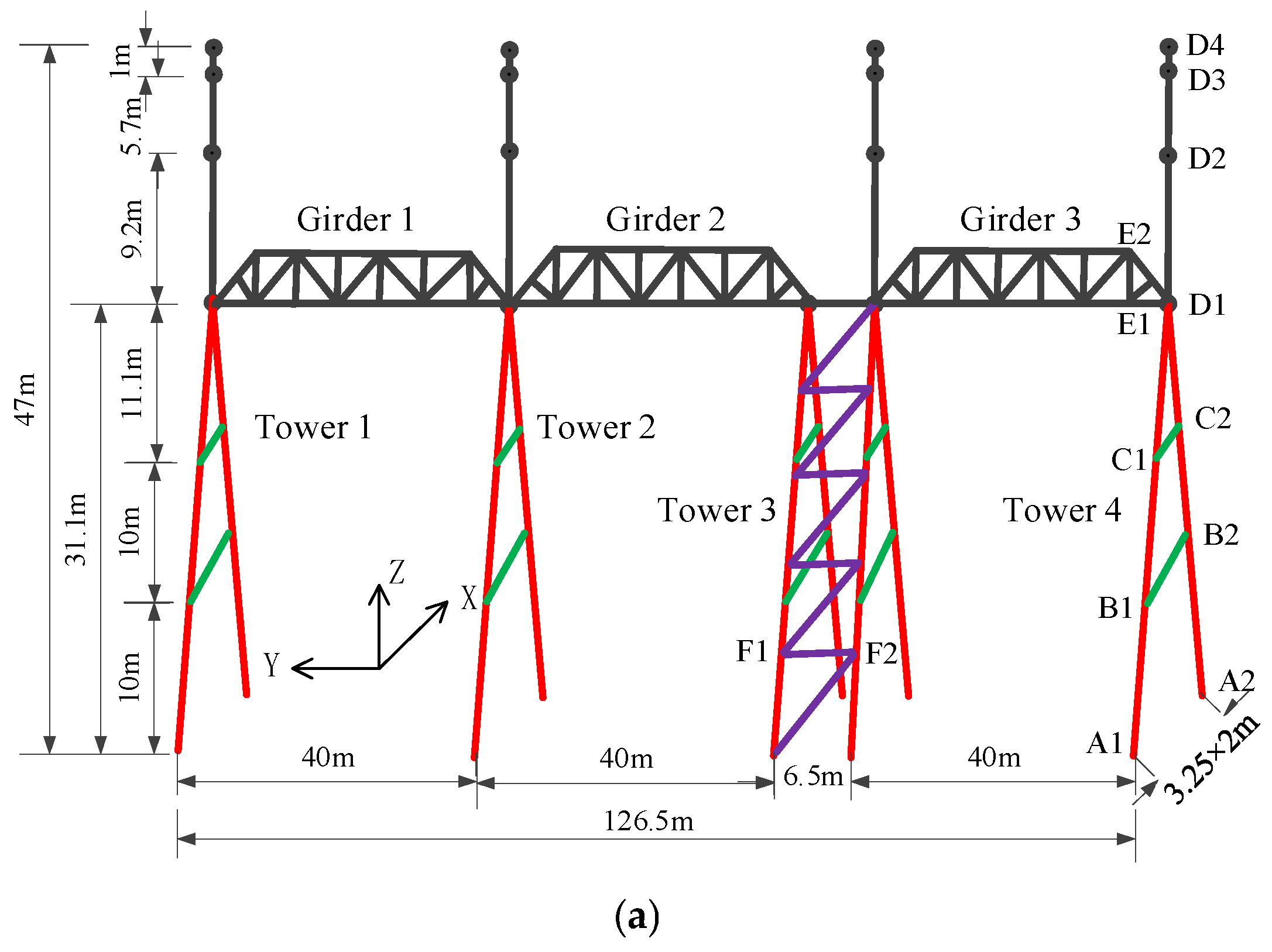
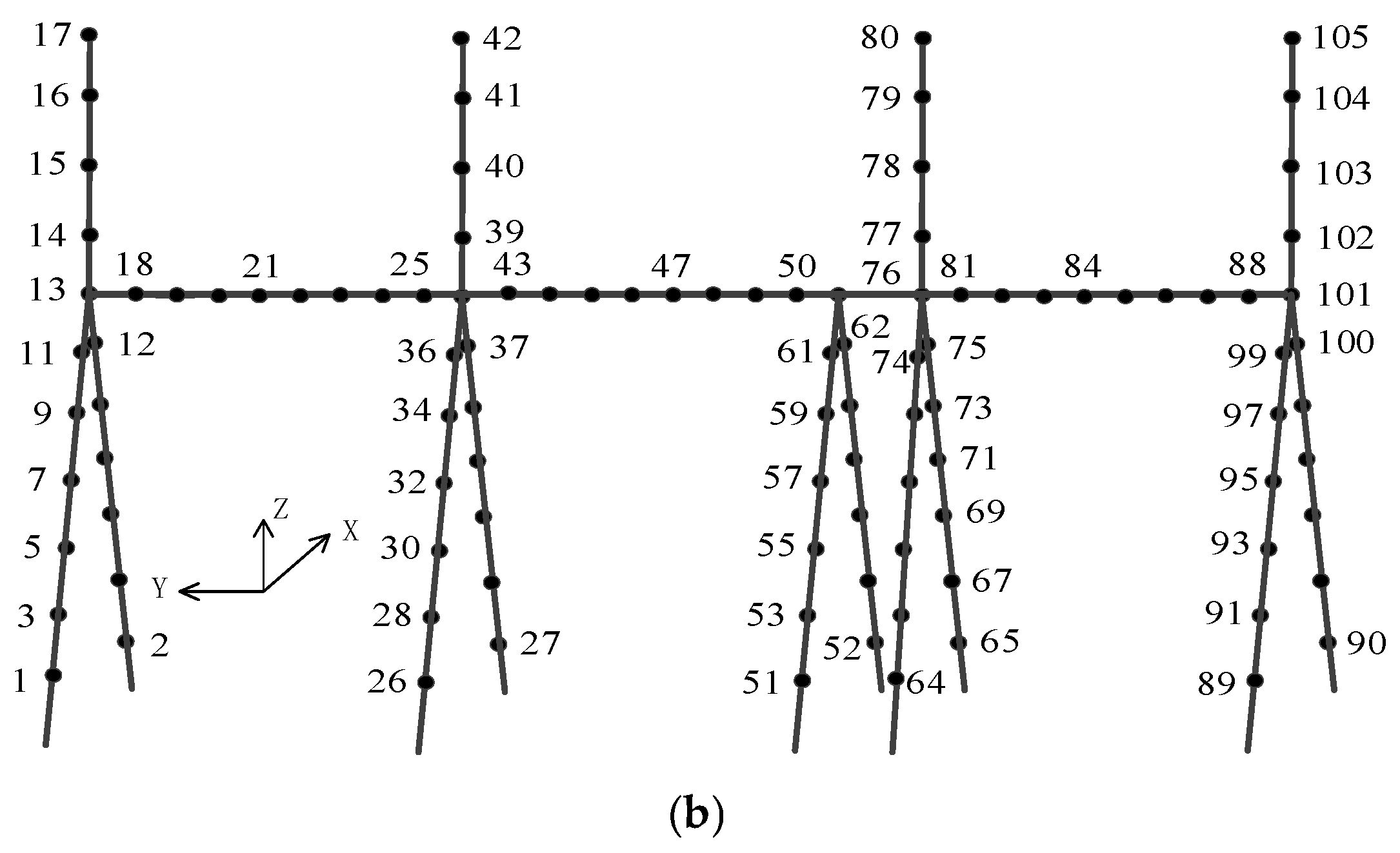
To validate the proposed non-stationary fluctuating wind field simulation method, this section conducts a simulation of the X-direction wind field for the three-span frame lightning-rod structure (Figure 3a) presented in Dong et al. [36]. The 105 wind-velocity simulation points adopted herein are plotted in Figure 3b (In the structural model, a global Cartesian coordinate system is defined relative to the structural geometry: the X-axis is perpendicular to the plane of the frames (corresponding to the along-wind direction), the Y-axis is parallel to the length direction of the girders (corresponding to the across-wind direction), and the Z-axis aligns with the vertical height of the towers). The simulation is implemented by programming in Matlab 2025a, and the computational environment is as follows: Intel (R) Core (TM) i5-14600KF CPU @ 3.50 GHz and 32 GB RAM (Intel, Santa Clara, CA, USA).

In the simulation, the target spectrum in the along-wind direction adopts the evolutionary spectrum S(ω, t) (Equations (30)–(32)) modulated from the Kaimal spectrum [37,38]. The time-varying mean wind speed is obtained by modulating the mean wind (Equations (33) and (34)), and the vertical variation of the mean wind speed follows the exponential wind profile (Equation (35)), as detailed below:

$$S(\omega , t)=|A(\omega , t){|}^{2}S(\omega )$$

(30)

$${\displaystyle \frac{\omega S(\omega )}{2\mathsf{\pi }{u_{*}}^2}}={\displaystyle \frac{200f}{{(1+50f)}^{5/3}}}$$

(31)

$$A(\omega , t)=\sqrt{{\displaystyle \frac{\tilde{U}(z, t)}{\overline{U}(z)}}{\left\{{\displaystyle \frac{1+50\frac{\omega z}{2\mathsf{\pi }\overline{U}(z)}}{1+50\frac{\omega z}{2\mathsf{\pi }\tilde{U}(z, t)}}}\right\}}^{5/3}}$$

(32)

$$\tilde{U}(z,t)=d(t)\overline{U}(z)$$

(33)

$$d(t)={\alpha }_0{t}^{{\beta }_0}{e}^{-\mathsf{\lambda }t}, {\alpha }_0>0, {\beta }_0, \mathsf{\lambda }\ge 0$$

(34)

$$\overline{U}(z)=U_r{({\displaystyle \frac{z}{10}})}^{\alpha }$$

(35)

where A(ω, t) is the modulation function, which is a coupled function of time and frequency; S(ω) is the Kaimal spectrum; f = nz/$\overline{U}(z)$ is the Monin coordinate; $\overline{U}(z)$ is the mean wind speed; n = ω/2π is the fluctuating-wind frequency; $u_{*}$ = K$\overline{U}(z)$/log(z/z₀) is the friction velocity, with K = 0.4 being the von Karman constant; z is the height of the simulation point above the ground; d(t) is the time-modulation function, and it can be shown from its derivative that it attains its maximum at t_max = β₀/λ; U₁₀ is the mean wind speed at z = 10 m, and U₁₀ = 20 m/s is adopted in this study; z₀ and α are the roughness length and terrain roughness exponent, respectively. For terrain category A, the Code for Wind-resistant Design of Highway Bridges specifies (JTG/T 3360-01-2018) [39] α = 0.12, and z₀ = 0.01 can be adopted [40].

Other basic parameters used in the simulation are listed in

Table 1. Basic computational parameters.

Parameters	Value	Parameters	Value
Cut-off frequency	ωu = 4π	Total simulation duration	T0 = 600 s
Number of frequency points	N = 1200	Number of time points	M = 2400
Frequency increment	Δω = ωu/N = 0.0105 rad/s	Time step	Δt = T0/M = 0.25 s
Shape parameter	β0 = 4	Peak time	tmax = 300 s
Modal order	NR = 3	Peak value	d(tmax) = 1
Adjustable parameter	κ = 0.8	Number of interpolation points	Nt = 30 and Nω = 20

. In this study, considering the flexibility of the three-span frame lightning-rod structure, its dominant natural frequencies are relatively low, with the first and second lateral bending frequencies being 0.75 Hz and 2.09 Hz [40], respectively. Consequently, ω_u = 4π rad/s (i.e., 2.0 Hz) was selected, which is sufficient to cover both the significant wind energy range and the primary modal frequencies. Furthermore, this value corresponds to the time step Δt = 0.25 s employed in the simulation (ω_u = π/Δt), thereby satisfying the Nyquist–Shannon sampling theorem to prevent frequency aliasing [41]. The selections of N_R, N_t, and N_ω will be further discussed in the next section.

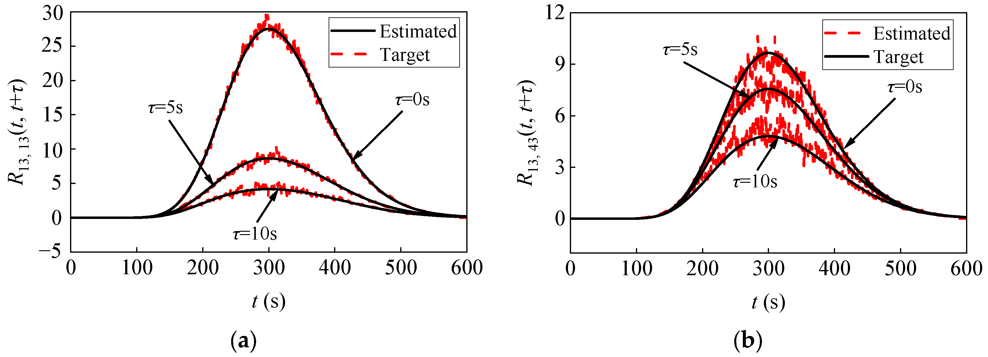
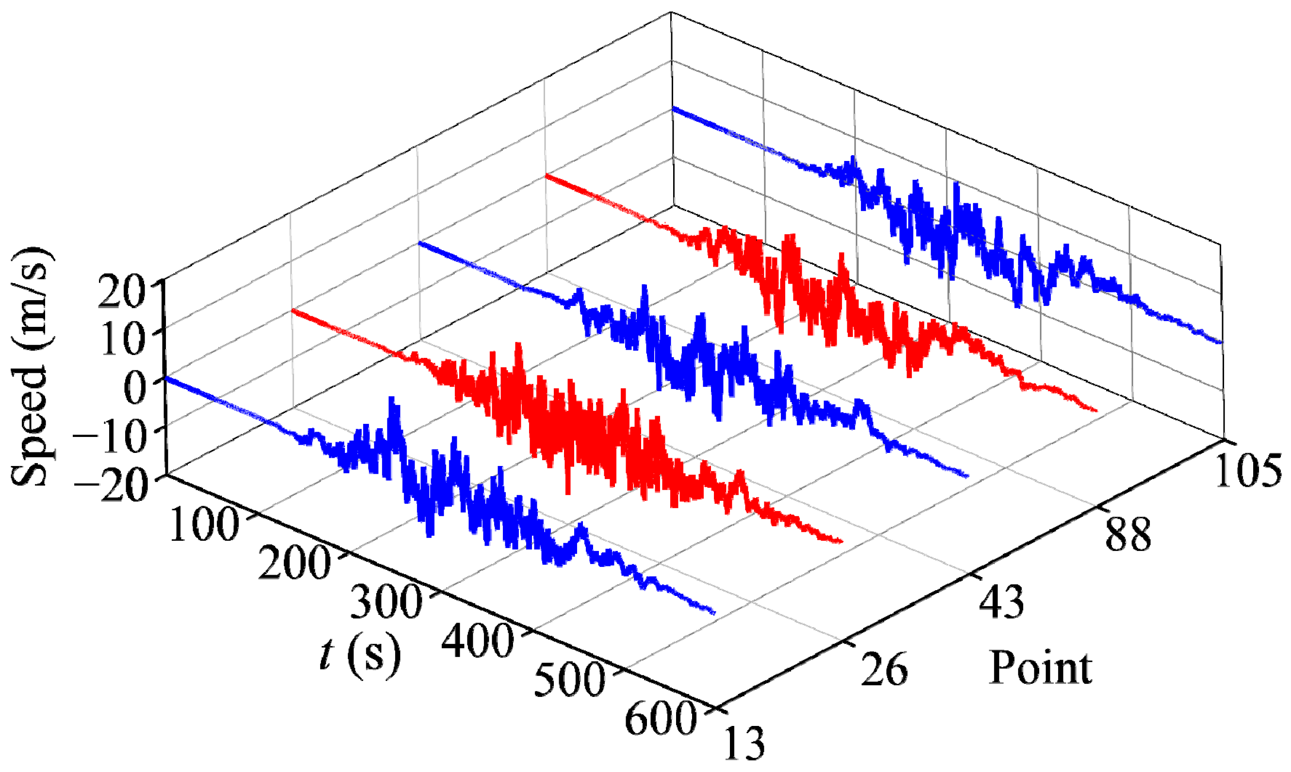
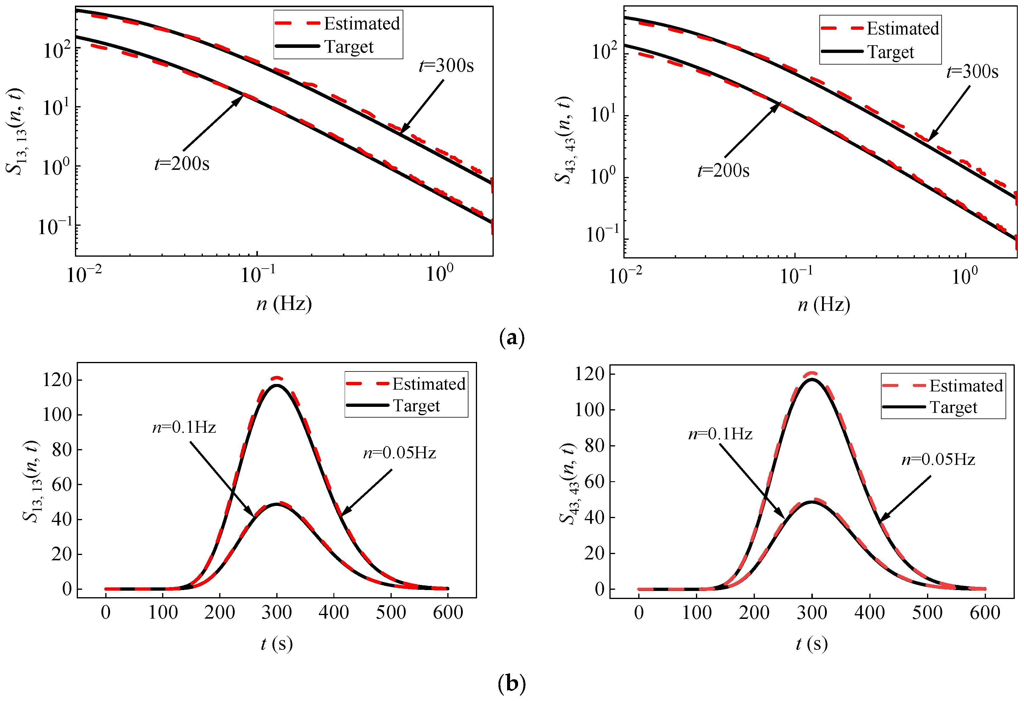
The 10 min along-wind fluctuating wind-velocity time histories at Point 13, 26, 43, 88, and 105 (Figure 3b) obtained from the present simulation are shown in Figure 4. In order to validate the effectiveness of the proposed method in simulating nonstationary fluctuating wind velocities, 2000 wind-speed samples are generated for Point 13 and Point 43, respectively, and the sample-averaged EPSD and correlation functions are then obtained accordingly (Equations (36) and (37)).

$${\overline{S}}_{\mathit{jj}}(\omega ,t)={\displaystyle \frac{1}{N_{\mathrm{samp}}}}{\displaystyle \sum _{r=1}^{N_{\mathrm{samp}}}{S}_{\mathit{jj}}^r(\omega ,t)}$$

(36)

$${\overline{R}}_{\mathit{jk}}(t,t+\mathsf{\tau })={\displaystyle \frac{1}{N_{\mathrm{samp}}}}{\displaystyle \sum _{r=1}^{N_{\mathrm{samp}}}E[{\mathrm{V}}_j^r(t){\mathrm{V}}_k^r(t+\mathsf{\tau })]}$$

(37)

where ${\overline{S}}_{\mathit{jj}}(\omega ,t)$ and ${\overline{R}}_{\mathit{jk}}(t, t+\mathsf{\tau })$ denote the sample-averaged EPSD and the auto-/cross-correlation function, respectively; N_samp is the number of samples; $S_{jj}^r$(ω, t) is the EPSD of the rth wind-speed sample; and $V_j^r$ and $V_k^r$(t + τ) are the wind speeds at the jth and kth measurement points at time instants t and t + τ in the rth sample, respectively.

Comparison with the target results (Figure 5 and Figure 6) indicates that the resulting mean EPSD and autocorrelation functions agree well with the targets. Owing to the large distance between Point 13 and Point 43, the cross-correlation function between the two points exhibits relatively large scatter, yet it still fluctuates around the target values. These results demonstrate that the proposed method has high fidelity and is capable of effectively simulating nonstationary fluctuating wind fields.

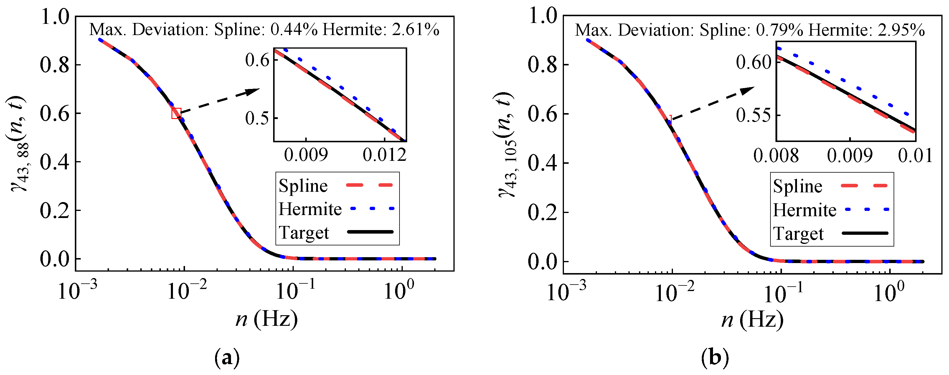
To demonstrate the superiority of Spline interpolation, Hermite interpolation is also adopted for comparison. The coherence functions at t = 300 s obtained by the two interpolation schemes are compared in Figure 7. As shown in Figure 7a, the maximum deviation of the coherence function for Point 43 and Point 88 from the Spline interpolation is less than 0.44%, whereas the Hermite interpolation reaches 2.61%. Similarly, in Figure 7b, the maximum deviations are 0.79% for Spline and 2.95% for Hermite for another group of points, indicating that the simulation method using Spline interpolation achieves higher accuracy than that using Hermite interpolation in reconstructing the time-frequency functions.

4.2. Error and Efficiency Analysis

It is clear that all errors in the simulation originate from the decoupling and interpolation-based reconstruction of the H matrix. The level of error is evidently related to the number of time-frequency interpolation points N_t and N_ω, as well as the retained modal order N_R used in reconstruction. The influence of these parameters can be analyzed using the error function E(N_t, N_ω, N_R) [29]:

$$E(N_t, N_{\omega }, N_R)={\displaystyle \frac{2}{m(m+1)}}{\displaystyle \sum _{j=1}^m{\displaystyle \sum _{k=1}^j\frac{{\displaystyle {\int }_0^{T_0}{\displaystyle {\int }_0^{{\omega }_u}\left|H_{\mathit{jk}}(\omega ,t)-{ H ˜}_{\mathit{jk}}(\omega ,t)\right|}}d\omega \mathit{dt}}{{\displaystyle {\int }_0^{T_0}{\displaystyle {\int }_0^{{\omega }_u}\left|H_{\mathit{jk}}(\omega ,t)\right|}}d\omega \mathit{dt}}}}$$

(38)

where H_jk(ω, t) and ${\tilde{H}}_{\mathit{jk}}(\omega ,t)$ represent the elements of the target and reconstructed lower triangular matrices obtained from the Cholesky decomposition, respectively. Consistent with the definition in Equations (1) and (2), m denotes the total number of simulation points, while j and k serve as the row and column indices, respectively.

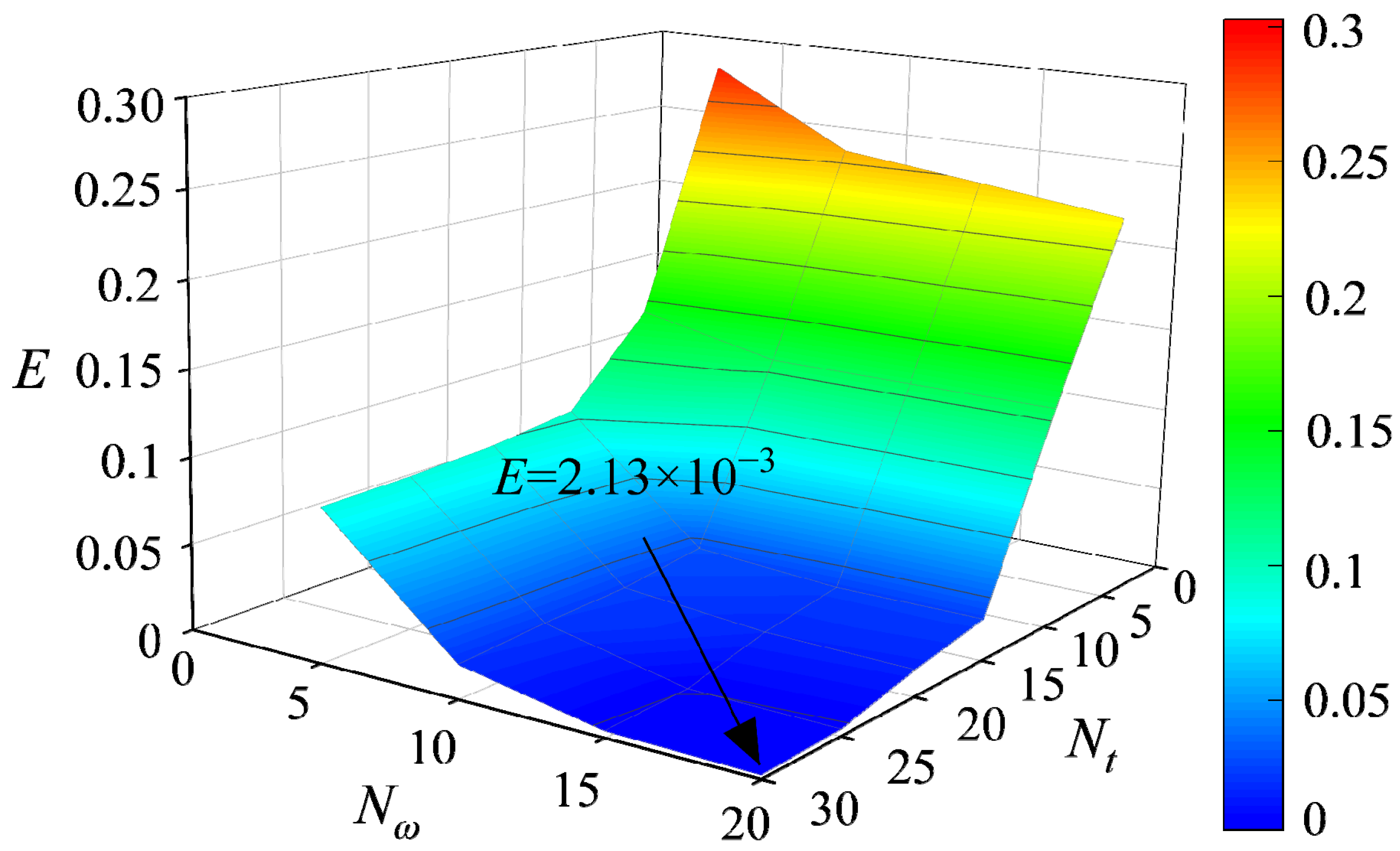
For the above numerical example, with N_R = 3, the simulation errors corresponding to different numbers of time-frequency interpolation points are shown in Figure 8. When N_t = 30 and N_ω = 20, the error E is only 2.13 × 10⁻³, which fully satisfies the computational requirement. Compared with performing the Cholesky decomposition on the full time-frequency matrix (N = 1200, M = 2400), or without truncating the modal order ($N_R^{max}$ = N_ω = 20), the computational costs of decomposition and decoupling are reduced by approximately 99.98% and 85.00%, respectively, leading to a significant improvement in simulation efficiency.

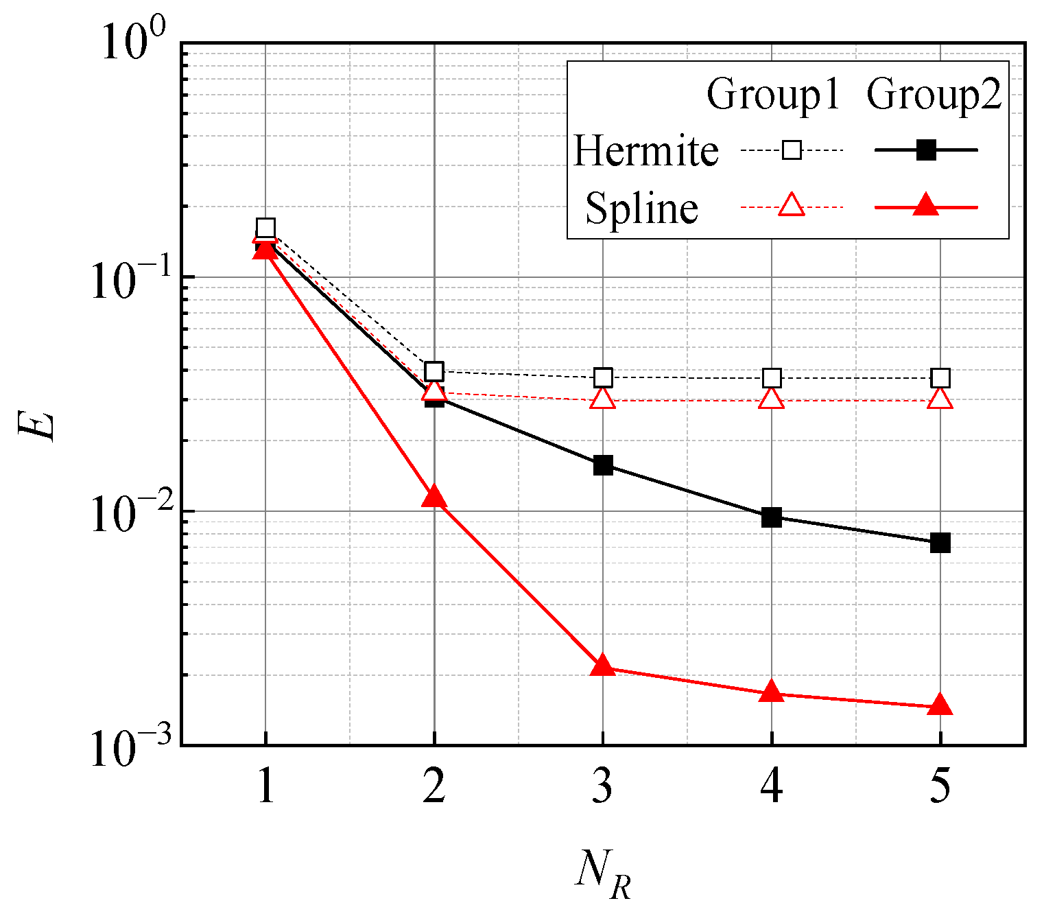
Two additional groups of time-frequency interpolation points are further selected for error comparison (Group 1: N_t = 15 and N_ω = 10; Group 2: N_t = 30 and N_ω = 20), and Hermite interpolation is again included as a benchmark. The results are presented in Figure 9. It is evident that, for a fixed group number of time-frequency interpolation points N_t and N_ω, Spline interpolation produces smaller errors than Hermite interpolation for all considered N_R. This advantage is particularly pronounced for Group 2: the error of the proposed method with N_R = 2 is close to that obtained using Hermite interpolation with N_R = 5, and with N_R = 3 the former becomes much smaller than the latter even at N_R = 5, providing a direct demonstration of the accuracy advantage of Spline interpolation.

In terms of computational efficiency, it can be deduced from Equations (12) and (25) that the number of interpolation and FFT operations required by the two methods are m(m + 1)N_R and m(m + 1)N_R/2, respectively. Therefore, reducing N_R from 5 to 2 or 3 decreases the computational effort associated with interpolation and FFT by approximately 60% and 40%, respectively. The detailed runtimes of each step are listed in

Table 2. Comparison of simulation time for different N_R values (unit: s).

Procedure	NR = 2	NR = 3	NR = 5	Time Ratio
Cholesky decomposition	0.22	0.22	0.22	1:1:1
Interpolation + decoupling	0.66	0.87	1.32	1:1.32:2.00
FFT	0.43	0.63	1.26	1:1.47:2.93
Total	1.31	1.72	2.80	1:1.31:2.14

Note: The values in the ‘Time ratio’ column represent the computational time of each case normalized by the time of the first case (the leftmost data column).

. Moreover, for fixed N_t and N_ω, even if the number of simulation points increases from 105 in this example to 500, the relative efficiency resulting from the reduced N_R remains unchanged. This indicates that the proposed method is more advantageous for large-scale wind-field simulations.

To further investigate the effects of N_t, N_ω, and N_R on simulation efficiency, an error threshold of E = 1.2% is adopted. Using Spline interpolation, the minimum required N_t and N_ω are determined for four cases with N_R = 2~5, while keeping N_t/N_ω = 1.5. The results are summarized in

Table 3. Comparison of runtime and error under different cases.

Parameters	NR = 2 Nt = 30, Nω = 20	NR = 3 Nt = 21, Nω = 14	NR = 4 Nt = 20, Nω = 13	NR = 5 Nt = 18, Nω = 12	Time Ratio
Cholesky decomposition (s)	0.22	0.12	0.09	0.07	1:0.55:0.41:0.32
Interpolation + decoupling (s)	0.66	0.70	0.83	1.00	1:1.01:1.20:1.45
FFT (s)	0.43	0.67	1.08	1.20	1:1.56:2.51:2.79
Total (s)	1.31	1.49	2.00	2.27	1:1.11:1.49:1.69
Simulation error E (%)	1.13	1.04	1.11	1.17	---

, where the step-by-step runtimes and the corresponding simulation errors are also provided.

As shown in Table 3, although the simulation errors in all four cases are approximately 1.2%, the case with N_R = 2 yields the shortest total runtime. With increasing N_R, even though N_t and N_ω gradually decrease, the total runtime still increases. This suggests that, under a fixed error level, N_R has a greater impact on the total runtime than N_t and N_ω. The reason is that the number of interpolation and FFT operations are directly proportional to N_R, and these two parts dominate the computational cost, whereas N_t and N_ω affect only the number of decompositions, whose cost is relatively small. Therefore, for large-scale wind-field simulations, reducing the modal order benefits more than reducing the number of time-frequency interpolation points in improving efficiency. This also highlights the importance of selecting an appropriate interpolation function, which allows a smaller N_R to be used while maintaining accuracy and thus enhances computational efficiency.

As shown in Figure 9, for the present example, the simulation error is close to 1.2% when N_R = 2 and becomes negligible for N_R = 3~5. To guide a rational choice of N_R, the average energy ratios of the first five modes of the temporal-averaged frequency correlation matrix R are listed in

Table 4. Average energy ratios of the correlation matrix R for different N_R values.

Modal Order NR	Average Energy Ratio (%)
1	99.06
2	0.93
3	4.11 × 10−3
4	2.21 × 10−5
5	1.33 × 10−7

, taking Group 2, i.e., N_t = 30 and N_ω = 20, as an example. It can be seen that when N_R = 1 the energy ratio already reaches 99.06%, indicating that almost all the energy of the correlation matrix R is concentrated in the first eigenmode. When N_R = 2, the cumulative energy exceeds 99.99%, and the energy in the higher modes could be neglected totally. Therefore, considering both accuracy and efficiency, N_R = 2 is recommended as the truncation order for this example, because the cumulative energy ratio of the modes of the correlation matrix R is at a high level (> 99.9%) while avoiding the additional computational cost induced by retaining excessive modes.

5. Conclusions

This study proposes a nonstationary wind-field simulation method based on POD decoupling and spline interpolation, which is applied to a three-span frame lightning-rod structure for validation. The influences of the parameters N_R, N_t, and N_ω on simulation error and efficiency are investigated comparatively with the Hermite-interpolation-based method. The results demonstrate the high efficiency and high fidelity of the proposed method. The main conclusions are as follows:

(1)

For the nonstationary fluctuating wind field simulated by the proposed method, the sample-averaged EPSD, correlation functions, and coherence functions show excellent agreement with the target values, verifying the effectiveness of the proposed method.

(2)

Compared with the Hermite-interpolation-based method, the proposed method achieves a pronounced improvement in computational efficiency. For the present example, using Spline interpolation with N_R = 2 attains an accuracy quite close to that achieved by Hermite interpolation with N_R = 5. The reduced N_R results in fewer POD-decoupling and FFT computations.

(3)

The number of POD-decoupling and FFT operations are directly related to N_R, and these two parts account for a larger portion of the total runtime than the other steps. Therefore, under the same error threshold, N_R has a greater impact on simulation efficiency than N_t and N_ω. A rational choice of N_R can be determined based on the cumulative energy ratio of the temporal-averaged frequency correlation matrix R, and it is recommended that the cumulative energy ratio reaches 99.9% to achieve a balance between accuracy and computational efficiency.

It should be noted that the time-varying mean wind employed in this study is artificially specified. Under this specific wind pattern, the Spline interpolation demonstrates superior simulation performance compared to the Hermite interpolation. Comparative analyses were also conducted using measured time-varying mean wind. It was observed that, due to the less pronounced time-varying characteristics of the measured wind compared to the artificially specified one, the advantage of Spline interpolation—while still observable—was less distinct. Consequently, the artificially specified time-varying mean wind was adopted in this study to better demonstrate the superiority of the Spline interpolation method.

Furthermore, future work will focus on the following aspects: First, the calculation of structural dynamic responses under non-stationary wind fields will be performed to analyze their characteristics, including displacement responses, internal forces, and time-frequency energy distributions. More importantly, the significant differences in dynamic response features between stationary and non-stationary wind excitations will be investigated.

References

1. Li, Y.L.; Zhou, S.H.; Qiang, S.Z. Three-dimensional fluctuating wind-field simulation for long-span cable-stayed bridges. China Civ. Eng. J. 2003, 36, 60–65. (In Chinese) [Google Scholar]
2. Hu, W.C.; Yang, Q.S.; Peng, L.L.; Liu, L.Y.; Zhang, P.F.; Li, S.P.; Wu, J. Non-stationary modeling and simulation of strong winds. Heliyon 2024, 10, e35195. [Google Scholar] [CrossRef] [Scilit] [PubMed]
3. Huang, Z.F.; Xu, Y.L.; Zhan, S. Conditionally simulating nonstationary typhoon winds with time-varying coherences for long-span bridges. J. Wind Eng. Ind. Aerodyn. 2021, 212, 104599. [Google Scholar] [CrossRef] [Scilit]
4. Cui, B.C.; Huang, P.; Xie, W. Fractal dimension characteristics of wind speed time series under typhoon climate. J. Wind Eng. Ind. Aerodyn. 2022, 229, 105144. [Google Scholar] [CrossRef] [Scilit]
5. Zhang, Y.X.; Wang, D.H.; Sun, C.; Fu, X. Probabilistic study on non-stationary extreme response of transmission tower under moving down burst impact. Structures 2024, 68, 107179. [Google Scholar] [CrossRef] [Scilit]
6. Huang, G.Q.; Zheng, H.T.; Xu, Y.L.; Li, Y.L. Spectrum models for nonstationary extreme winds. J. Struct. Eng. 2015, 141, 04015010. [Google Scholar] [CrossRef] [Scilit]
7. Jiang, F.Y.; Zhang, M.J.; Li, Y.L.; Yan, T.Y.; Zhang, J.X. Field measurement analysis of wind parameters and nonstationary characteristics in mountainous terrain: Focusing on cooling windstorms. J. Wind Eng. Ind. Aerodyn. 2022, 230, 105175. [Google Scholar] [CrossRef] [Scilit]
8. Wang, Y. Field Measurement and Simulation of Nonstationary Winds at a Bridge Site in a Mountainous Canyon Area. Master’s Thesis, Chongqing Jiaotong University, Chongqing, China, 2023. (In Chinese) [Google Scholar]
9. Chen, X.; Kareem, A. Proper orthogonal decomposition-based modeling, analysis, and simulation of dynamic wind load effects on structures. J. Eng. Mech. 2005, 131, 325–339. [Google Scholar] [CrossRef] [Scilit]
10. Tao, T.; Xu, Y.L.; Huang, Z.; Zhan, S.; Wang, H. Buffeting analysis of long-span bridges under typhoon winds with time-varying spectra and coherences. J. Struct. Eng. 2020, 146, 04020255. [Google Scholar] [CrossRef] [Scilit]
11. Yao, C.Y. Time-Domain Simulation and Analysis of Nonstationary Buffeting of a Long-Span Suspension Bridge Under Typhoon Winds. Master’s Thesis, Southeast University, Nanjing, China, 2019. (In Chinese) [Google Scholar]
12. Li, X.L. Study on Buffeting Responses of Long-Span Bridges Under Fully Nonstationary Winds. Master’s Thesis, Sichuan Agricultural University, Ya’an, China, 2023. (In Chinese) [Google Scholar]
13. Kareem, A. Numerical simulation of wind effects: A probabilistic perspective. J. Wind Eng. Ind. Aerodyn. 2008, 96, 1472–1497. [Google Scholar] [CrossRef] [Scilit]
14. Chen, X.; Jiang, Y.; Zhao, N.; Jia, S.; Wang, X.; Tan, S. Simulation of stationary and nonstationary wind velocity field along a long-span bridge using a numerical truncation method. J. Wind Eng. Ind. Aerodyn. 2022, 231, 105206. [Google Scholar] [CrossRef] [Scilit]
15. Gao, Y.; Wu, Y.; Li, D.; Liu, H.; Zhang, N. An improved approximation for the spectral representation method in the simulation of spatially varying ground motions. Probabilistic Eng. Mech. 2012, 29, 7–15. [Google Scholar] [CrossRef] [Scilit]
16. Tao, T.Y.; Wang, H.; Kareem, A. Reduced-Hermite bifold-interpolation assisted schemes for the simulation of random wind field. Probabilistic Eng. Mech. 2018, 53, 126–142. [Google Scholar] [CrossRef] [Scilit]
17. Liu, S.Y.; Peng, L.L.; Liu, J.; Zhao, S.; Jiang, Z.M. Spectral representation-based efficient simulation method for fully non-stationary spatially varying ground motions. Soil Dyn. Earthq. Eng. 2022, 161, 107436. [Google Scholar] [CrossRef] [Scilit]
18. Bao, X.M.; Li, C.Y. Fast simulation of non-stationary wind velocity based on time-frequency interpolation. J. Wind Eng. Ind. Aerodyn. 2019, 193, 103982. [Google Scholar] [CrossRef] [Scilit]
19. Han, H.; Li, C.; Li, J. Fast simulation of large-scale nonstationary wind velocities based on adaptive interpolation reconstruction scheme. Wind Struct. 2021, 33, 55–69. [Google Scholar]
20. Jiang, Y.; Zhao, N.; Peng, L.; Xin, J.; Liu, S. Fast simulation of fully nonstationary wind fields using a new matrix factorization assisted interpolation. Mech. Syst. Signal Process. 2022, 172, 108973. [Google Scholar] [CrossRef] [Scilit]
21. Li, C.; Chen, L.; Cao, L. High-efficiency simulation of nonstationary wind velocity using diagonal POD of decomposed time-frequency interpolation node spectrum matrices. J. Wind Eng. Ind. Aerodyn. 2023, 233, 105314. [Google Scholar] [CrossRef] [Scilit]
22. Yang, J.N. Simulation of random envelope processes. Sound Vib. 1972, 21, 73–85. [Google Scholar] [CrossRef] [Scilit]
23. Wittig, L.E.; Sinha, A.K. Simulation of multicorrelated random processes using the FFT algorithm. J. Acoust. Soc. Am. 1975, 58, 630–634. [Google Scholar] [CrossRef] [Scilit]
24. Li, Y.; Kareem, A. Simulation of multi-variate non-stationary random processes by FFT. J. Eng. Mech. 1991, 117, 1037–1058. [Google Scholar]
25. Spanos, P.D.; Failla, G. Evolutionary spectra estimation using wavelets. J. Eng. Mech. 2004, 130, 952–960. [Google Scholar] [CrossRef] [Scilit]
26. Huang, G.Q. An efficient simulation approach for multivariate nonstationary process: Hybrid of wavelet and spectral representation method. Probabilistic Eng. Mech. 2014, 37, 74–83. [Google Scholar] [CrossRef] [Scilit]
27. Lee, D.D.; Seung, H.S. Learning the parts of objects by non-negative matrix factorization. Nature 1999, 401, 788–791. [Google Scholar] [CrossRef] [Scilit]
28. Jiang, Y.; Zhao, N.; Peng, L.; Zhao, L.; Liu, M. Simulation of stationary wind field based on adaptive interpolation-enhanced scheme. J. Wind Eng. Ind. Aerodyn. 2019, 195, 104001. [Google Scholar] [CrossRef] [Scilit]
29. Tao, T.; Wang, H.; Zhao, K. Efficient simulation of fully non-stationary random wind field based on reduced 2D Hermite interpolation. Mech. Syst. Signal Process. 2020, 150, 107265. [Google Scholar] [CrossRef] [Scilit]
30. Zhao, N.; Jiang, Y. Fast simulation of nonstationary wind velocity fields by POD. Wind Eng. Ind. Aerodyn. 2021, 219, 104798. [Google Scholar] [CrossRef] [Scilit]
31. Priestley, M.B. Evolutionary spectra and nonstationary processes. J. R. Stat. Soc. Ser. B 1965, 27, 204–237. [Google Scholar] [CrossRef] [Scilit]
32. Deodatis, G. Simulation of ergodic multivariate stochastic processes. J. Eng. Mech. 1996, 122, 778–787. [Google Scholar] [CrossRef] [Scilit]
33. Solari, G. Turbulence modeling for gust loading. J. Struct. Eng. 1987, 113, 1550–1564. [Google Scholar] [CrossRef] [Scilit]
34. Wu, F.B.; Xu, Z.L.; Zhao, N.; Chen, X.W.; Wang, X.; Wu, Y. Efficient simulation of fully nonstationary wind velocity field by an enhanced numerical truncation method. J. Wind Eng. Ind. Aerodyn. 2023, 242, 105593. [Google Scholar] [CrossRef] [Scilit]
35. Chand, A.K.B.; Kapoor, G.P. On cubic Hermite coalescence hidden variable fractal interpolation functions. Appl. Math. -A J. Chin. Univ. 2015, 30, 55–76. [Google Scholar]
36. Dong, X.S.; Zhang, J.F.; Yang, Y.; Guan, P.W. Wind-induced responses of substation lattice lightning rods. Struct. Eng. 2020, 36, 106–113. (In Chinese) [Google Scholar]
37. Li, J.H.; Wu, C.P.; Chen, S.S. Numerical simulation of nonstationary fluctuating wind velocities in downbursts. J. Vib. Shock 2014, 33, 54–60. (In Chinese) [Google Scholar]
38. Kaimal, J.C. Spectral characteristics of surface-layer turbulence. Q. J. R. Meteorol. Soc. 1972, 98, 563–589. [Google Scholar] [CrossRef] [Scilit]
39. JTG/T 3360-01-2018; Code for Wind-Resistant Design of Highway Bridges. China Communications Press: Beijing, China, 2018.
40. Dong, X.S.; Zhang, J.F.; Yang, Y.; Guan, P.W. Analysis of correlation parameters of turbulence intensity of fluctuating wind. Struct. Eng. 2019, 35, 155–160. (In Chinese) [Google Scholar]
41. Shinozuka, M.; Deodatis, G. Simulation of stochastic processes by spectral representation. Appl. Mech. Rev. 1991, 44, 191–214. [Google Scholar] [CrossRef] [Scilit]
Figure 1. Schematic illustration of the decoupling, interpolation, and reconstruction procedure.
Buildings 16 00804 g001
Figure 2. Comparison between Spline interpolation and Hermite interpolation.
Buildings 16 00804 g002
Figure 3. Three-span frame lightning-rod structure [36]: (a) Structural configuration; (b) Layout of simulation points.
Buildings 16 00804 g003aBuildings 16 00804 g003b
Figure 4. Along-wind fluctuating wind-velocity time histories.
Buildings 16 00804 g004
Figure 5. Comparison of EPSD slices: (a) Frequency domain; (b) Time domain.
Buildings 16 00804 g005
Figure 6. Validation of correlation functions: (a) Autocorrelation at Point 13; (b) Cross-correlation between Point 13 and Point 43.
Buildings 16 00804 g006
Figure 7. Comparison of coherence functions at t = 300 s: (a) Point 43 and Point 88; (b) Point 43 and Point 105.
Buildings 16 00804 g007
Figure 8. Influence of the number of time-frequency interpolation points on simulation accuracy.
Buildings 16 00804 g008
Figure 9. Comparison of simulation errors obtained by the two interpolation methods.
Buildings 16 00804 g009