Article

Intelligent Prediction and Optimization of Concrete Resource Mismatch in China’s Construction Industry—An Explainability Analysis Based on XGBoost-SHAP


Department of School of Business Administration, Liaoning Technical University, Huludao 125105, China
*
Author to whom correspondence should be addressed.
Buildings 2026, 16(2), 316; https://doi.org/10.3390/buildings16020316
Submission received: 20 November 2025 / Revised: 25 December 2025 / Accepted: 7 January 2026 / Published: 12 January 2026
(This article belongs to the Section Building Energy, Physics, Environment, and Systems)

Abstract

Concrete is the most carbon-intensive sector of building and construction. It leads to severe project results due to poor distribution. Cost increases, project delays, and the production of greenhouse gases. Machine learning techniques may be helpful when looking at complicated construction data; however, the issue with machine learning is the “black box” issue, and this causes a big trust issue between the project manager and the prediction model, and, thus, no one will make a choice based on the model. For that, we have Explainable AI. It brings together the power of XGBoost’s predictions with the interpretability of SHAP. We used it on the data from our four mega projects, and we got a very nice R-squared of 0.922. By looking at the SHAP analysis result, we can see that Electricity Consumption per Unit Concrete (ECUC) is the main driver, and there is a threshold for ECUC, which is 40.3 kWh/m3. If ECUC is greater than 40.3 kWh/m3, then resource waste will increase in a nonlinear way. And we transform these conclusions into a three-level optimization plan to indicate that it may be possible to reduce resources that do not fit by 38.6%. This study gives a new “prediction–interpretation–optimization” model, instead of prediction only, it gives practical and transparent decisions in construction that can use resources properly.

1. Introduction

In the processes of building infrastructure construction, the efficiency of construction project resource utilization is an important bottleneck for the cost of construction projects, construction period, and construction quality of the construction project [1]. In terms of construction materials, the most commonly used single material is concrete, with the largest carbon footprint. If its usage changes, there will be a series of chain reactions such as resource waste, higher costs, and greater environmental burden. So, it is important to make an accurate prediction of daily concrete consumption to achieve lean management of resources, reduce waste, and minimize environmental pollution [2].
The traditional management method is based on the data of the past, and also uses a linear equation to represent the situation of many things on the construction site, which is too complex, leading to poor resource allocation of concrete [3]. This sort of plan tends to presume a simple, straight-line relationship between different variables that is inadequate for the complex construction setting. To address the limitations of traditional linear models, existing research has introduced machine learning (ML) techniques, particularly ensemble methods such as XGBoost, which have a superior ability to capture complex nonlinear relationships in high-dimensional building data [4].
Currently, Explainable Artificial Intelligence (XAI) has demonstrated critical value across multiple engineering disciplines. For instance, in structural engineering, studies seek to leverage XAI to process complex data in support of structural health monitoring and safety assessment [5]; in geotechnical engineering, efforts have focused on improving both predictive accuracy and interpretability in simulating complex processes such as debris flows by integrating physical mechanisms with data-driven approaches such as the MGDD model [6] or the CNN–GRU–CHIO hybrid model [7]; in the power system field, research has utilized frameworks including SHAP to quantify the individual impact of diverse factors on transient grid stability, thereby explaining the outputs of highly accurate artificial neural network (ANN) models [8].
Therefore, this study, while exploring the impact of key factors on concrete resource misallocation, further delves into quantifying the interaction effects among multiple factors and their synergistic influence on the misallocation outcome, thereby providing a new perspective for the fine-grained management of multi-variable coordination and regulation. This paper will address two research questions as follows:
(1)
How can we build a model that can precisely predict daily concrete consumption?
(2)
How can we explain the internal decision-making mechanism of this prediction model and propose corresponding resource optimization strategies?
The subsequent structure of this article is arranged as follows: Section 2 introduces the relevant literature. Section 3 elaborates on the research methods and design framework. Section 4 focuses on the analysis of the research results. The discussion is presented in Section 5. Section 6 summarizes the research conclusions and puts forward suggestions for future research directions.

2. Literature Review

2.1. Construction Engineering Resource Management

Construction engineering resource management is a basic part of the national economy and a key part of the system for livelihood security [9]. It indirectly affects the overall engineering project achievement efficiency [10]. However, with the gradual increase in the scale and overall engineering project difficulty levels [11], resource management is subject to two difficulties. On the one hand, the dynamic volatility and nonlinearities within the construction environment and resource requirements increase more and more visibly [12]. On the other hand, general resources—materials with the greatest scale and greatest impact on carbon emissions—display more considerable consumption deviations and transmission effects [13]. As for the decision-making time and information asymmetry, the traditional construction engineering resource management model leads to greater efficiency in the management of construction engineering resources.
Based on the problems mentioned above, the research community began to have a change in paradigm from a data-driven approach to a management model with better cooperation between the demand forecast and supply chain [14]. Even so, the shift from experience-based to data-informed strategies is not without limitations in the current research [15]. The methodological landscape remains one-parameter optimization and static models, unable to account for the dynamic nature of construction projects [16]. There may be a push for machine learning to be used for things like resource management and scheduling, but for the most part, we are still looking at static analysis and risks after the fact. This current approach is lacking in its ability to predict such crucial issues as suppl–demand imbalance and cascade failures [17] proactively. And, thus, a gap between pre-cognition and pre-acting. It is in such a context that this research is made in order to contribute to filling three main gaps, which are the lack of proactive predictive functions in the resource discordance, not enough investigation into the dynamic multi-factor process, and failing to incorporate data-driven solutions for practical management.

2.2. Machine Learning for Construction Resource Prediction

Data-driven change makes machine learning the highlight of study materials concerning construction resource estimates. It came out of the initial reliance on linear regression, time-series analysis [18]. Though it is important, it does not describe a true nonlinear relationship within architectural activities [19]. The advancement in the area of ensemble learning and deep learning makes it feasible to use more sophisticated methods, such as Random Forests, support vector machines, and different types of neural networks [20] on the multi-source high-dimensional datasets collected by the sensor network and the project management software [21]. Among them, the ensemble method XGBoost has been found to perform better with more structured tabular types of data, which is often what resource management tasks use [22,23]. XGBoost is fast on sparse data and supports missing values [24]. The regularization parameters of XGBoost for L1 and L2 would be fixed to tackle small projects so that we could generalize [25]. And its gradient boosting framework was very good for modeling the nonlinear interactions of activities and resources [26]. It is also computationally efficient enough to meet the tight time limits of project management [27].
XGBoost has a higher predictive power and relative precision when compared to the old methods, even if the “black-box” approach of XGBoost might still be a huge stumbling block when it comes to implementation, since managerial support is necessary in order to put these predictions into action. Therefore, having a model that has very good predictive power does not close the trust gap, and explaining the model’s outputs is needed so that it can be used in construction resource management.

2.3. Interpretive Path of XAI

Explainable Artificial Intelligence (XAI), which is a kind of artificial intelligence technology that makes machine learning models more transparent and trustworthy. The main idea of the method of XAI is global–local view joint analysis to achieve a transparent explanation of complex models’ behavior [28] and to create a credible link between the output of the algorithm and the manager’s cognitive system [29]. In the field of construction engineering resource management, the preliminary exploration of XAI has produced some results. Researchers are now starting to use SHAP to figure out which things matter the most when making choices about using resources and also to see how well different ways of explaining things work in this area [30]. These works will be the first steps towards transforming XAI from an idea into a tool to improve the credibility of construction decision support systems [31].
Though there are some initial developments, applying XAI to building engineering is still limited. The main limitation is that the existing XAI methods are mostly static explanations, and no dynamic explorations for multiple factors are made. And then there is also just that appearance that it does not have a clear path of being able to take ideas from XAI and actually making them something that managers can use to make their decisions. Such deficiencies make the existing XAI unable to cater to the complex needs of construction resource management. To solve the above problems, there are main gaps in this research that need to be addressed: improving static explanation, studying the dynamic interaction of multiple factors, creating a full explanation for the conversion from management strategy to management strategy, improving trustworthiness, and using engineering scenarios for more complex management processes.

3. Methodology and Design

3.1. Data Sources and Processing

3.1.1. Data Resource

To ensure the authority, representativeness, and fullness of the research data, four large-scale construction projects were selected as the main case studies in this study: the Shanghai Tower, Beijing Daxing International Airport, the Hong Kong–Zhuhai–Macao Bridge, and the affordable housing in the Xiong’an New Area. A multi-dimensional data support system was built by integrating macro statistical data, industry standards, and scientific monitoring data from different dimensions. The specific data sources used in this research are comprehensively summarized in Table 1.
The integration of these multi-source datasets provides a solid and multi-dimensional data support for the analysis of concrete consumption, and the research results are both academic and practical.

3.1.2. Data Collection and Preprocessing

For this research, four key projects were selected: the Shanghai Tower project, the Beijing Daxing International Airport project, the Hong Kong–Zhuhai–Macao Bridge project, and the Rongdong resettlement housing project for the Xiong’an New Area. In general, construction sites tend to shut down their concrete pouring activities during statutory holidays and therefore generate no construction data. Table 2 lists the periods and the volume of the data for each project.
Based on existing research [32,33], this study takes construction technology, supply chain, environment, labor, schedule and equipment as the analysis framework, and selects 12 key influencing factors as independent variables (in Table 3).
A targeted processing strategy was adopted to address data quality issues, including missing data, heterogeneity, and outliers. For the minimal missing continuous data (e.g., meteorological data, accounting for <2% of the dataset), mean imputation was applied. Data on personnel allocation were confirmed and filled through project documentation. Categorical variables were standardized through one-hot encoding or numerical mapping based on their attributes. Outliers, identified via interquartile range (IQR) analysis, were winsorized (capped at the 1st and 99th percentiles) to mitigate their impact while preserving data integrity, ensuring the processed data met the requirements for model construction.
To ensure the stability and convergence efficiency of the prediction model, data standardization was performed on the continuous numerical variables. They were transformed into a distribution with a mean of 0 and a standard deviation of 1, avoiding the influence of special values on the model’s objective function. The standardization was applied using the Z-score method, as defined in Equation (1):
Z = X μ / σ a
where X is the original feature value, μ is the mean of the feature calculated from the training set, and σ is its standard deviation. Crucially, the parameters ( μ and σ ) for standardization were estimated exclusively from the training dataset. The same parameters were then applied to transform both the validation and test sets. This approach effectively prevents information leakage from future time points, ensuring the authenticity and reliability of the model performance evaluation results. All continuous independent variables defined in Table 3, including ECUC, DTEC, DAT, DRL, ADD, SD, DPEQ, and EUCPU, underwent this standardization process.
Ultimately, the high-quality dataset, after cleaning, restructuring, and standardization, laid a solid foundation for subsequent models to achieve precise predictions and machine learning interpretations.

3.1.3. Hyperparameter Tuning and Model Training Strategy

For the machine learning model to function properly and dependably, this study carried out extensive hyperparameter optimization. Using modern Bayesian optimization methods, it is applied to all stages of model training and verification.
(1)
Definition of Hyperparameter Space
According to the working principle of the XGBoost algorithm and a few references, as well as a few initial experiments we performed, we selected 7 hyperparameters that are more influential on the model’s performance, which are listed in Table 4. These control how complicated a model we will allow, how much we let the model learn, and how much regularization we put on it.
(2)
Bayesian Optimization Based on TPE
In this study, we will be using the TPE tree-structured Parzen estimator as an optimizer to tune the hyperparameters. Compared to Grid Search and Random Search, TPE can create an estimate with a probabilistic model to separate the high-performing hyperparameters from the low-performing ones and direct the search better. It does a really good job at optimising models like XGBoost, which need many resources to compute.
(3)
Time-Series Validation and Model
To strictly avoid data leakage and simulate real-world prediction scenarios, a time-series cross-validation (TSCV) strategy was employed in the optimization process. Specifically, 5-fold validation was performed by sequentially sliding the time window on the training set (accounting for the first 80% of the full dataset’s time series), ensuring that the time points of the validation set always follow those of the training set. The optimization objective was to maximize the average coefficient of determination (R2) across the 5 folds. The TPE process ran for 100 iterations, and the hyperparameter combination with the best performance on the validation set was ultimately selected. The final model was retrained on the complete training set and evaluated on a strictly chronologically partitioned test set (the last 20% of the data).

3.2. Research Framework and Research Method

3.2.1. Research Framework

To address the problem of uneven supply of concrete resources in construction projects, this study combines the research methods mentioned above, and the specific research process is shown in Figure 1.
The first step is to collect and process various sources of construction information. In this stage, the entire collection, cleaning, and feature engineering were performed for multi-source raw data of 4 projects to form a high-quality structured dataset to build a solid foundation of data for subsequent analysis, based on the driving factors of core resource demand and interaction mechanism analysis. Phase is mainly used to build and improve the daily concrete consumption prediction model with the XGBoost algorithm. The R2 result is 0.922. The prediction effect is better than the benchmark, and it can provide a good quantitative basis for resource management. The daily concrete consumption prediction model is built by the XGBoost algorithm. This stage adopted Explainable AI (XAI) technology, such as SHAP technology, to reveal the model’s inner decision-making process, identify the ranking of feature importance, nonlinear threshold effect, and the interactions among critical factors, and, finally, explained the decision-making logic of the model with SHAP explainability technology. The last step translated the mechanistic information of SHAP analysis into a feasible 3-layer optimization strategy system that could provide specific decision-making support for different management levels to minimize resource mismatch efficiently.

3.2.2. Research Method

(1)
Prediction Model based on XGBoost
The eXtreme Gradient Boosting (XGBoost) algorithm was selected to develop the daily concrete consumption prediction model [34]. As shown in Equation (2):
O b j ( θ ) = l ( θ ) + Ω ( θ )
l ( θ ) quantifies the discrepancy between predicted and observed values, while Ω ( θ ) serves as the regularization component, crucial for controlling model complexity. The complexity Ω ( f k ) for an individual tree is typically computed using Equation (3), which penalizes based on the number of leaf nodes T and the magnitude of their weights ω :
Ω ( f k ) = γ T + 1 2 λ ω 2
Consolidating these elements, the overall objective function minimized during the training process for the additive model is presented in Equation (4):
O b j ( θ ) = i = 1 n l ( y i , y ̑ i t ) + k = 1 t Ω ( f k )
The predictive performance of the optimized XGBoost model was fully tested through the following three indicators: Mean Absolute Error (MAE), Root Mean Squared Error (RMSE), and the coefficient of determination ( R 2 ). An R 2 value closer to 1 signifies a superior model fit. The mathematical expressions for these criteria are presented below:
O b j ( θ ) = i = 1 n l ( y i , y ̑ i t ) + k = 1 t Ω ( f k )
R S M E = 1 n i = 1 n y i y ̑ i 2
R 2 = 1 i = 1 n y i y ̑ i 2 i = 1 n y ¯ i y i 2
(2)
Mechanism Interpretation using SHAP
SHAP is a game-theory-based method that links optimal credit allocation with local explanation [35], and it presents a unified measure of feature importance that is both globally consistent and locally accurate. It is mathematically defined in Equation (8) as follows:
Φ i = S F \ { i } S ! F S 1 ! F ! f S { i } X S { i } f S X S
where F is the set of all features, S is a subset of features excluding i, S is the size of subset S , and f s x s is the prediction model trained only on the subset of features S . The term f S { i } X S { i } f S X S represents the marginal contribution of a feature i when added to the subset S .
The application of SHAP in this study was conducted at two levels to achieve comprehensive interpretability.
(1)
Global Interpretability
To assess the overall influence of each driving factor on daily concrete consumption, the mean absolute SHAP value ( Φ i ) was computed for every feature across the entire dataset.
(2)
Local Interpretability and Nonlinear Effect Analysis
In addition to the global ranking, SHAP dependence plots were also generated to reveal the fine nonlinear relationship between a certain feature and the model output. The show details of SHAP values, that is, the impact on prediction, of a single feature changing with the change in actual values. This analysis is helpful for exploring threshold effects and interaction effects.
(3)
The Generalized Additive Model
GAM stands for Generalized Additive Model, and this is a general framework for a variety of statistical models that generalizes linear models when it comes to allowing nonlinear relationships between the response and predictor variables using smooth functions [36]. A general form for GAM can be written as follows:
g E y = β 0 + f 1 x 1 + f 2 x 2 + + f p x p
where g is the link function, E y is the expected value of the response variable, β 0 is the intercept, and each f j x j is a smooth function (typically represented by regression splines) that captures the nonlinear effect of the predictor x j on the response.
GAM is referred to as a smooth function that represents the nonlinear effect exerted by a predictor on the response. In the current research work, the application of GAM was utilized for the purpose of explaining and describing the nonlinear associations among important features and SHAP values. The smooth functions derived from the GAM analysis helped to explain the complex and non-monotonic behaviors outlined by the XGBoost-SHAP analysis.

4. Research Result

4.1. Comparative Performance Evaluation of Prediction Models

To scientifically assess predictive ability and generalizability and strictly avoid overfitting resulting from data leakage within this context, this section uses a time-series split validation for model evaluation. In this split validation exercise, the dataset is segregated along the time axis, with the first 80% used for training the model and the next 20% for model testing on a time-series split validation. It can thus test the ability to predict for the forecast model on past observations. A comparison among the three selected algorithms was made: Random Forest (RF), Linear Regression (LR), Multi-Layer Perceptron (MLP), and XGBoost. Table 5 highlights the testing performances for all three models on time-series split validation.
Overall Performance: XGBoost > MLP > RF ≈ LR. When considering all the models comprehensively, XGBoost is the most optimal, with the highest R2 value, the lowest error indicators for all metrics, and the best prediction accuracy and stability. MLP performs slightly inferior to XGBoost, with an R2 value close to XGBoost, but its various error metrics are slightly higher than XGBoost, and still a competitive model. Random Forest (RF) is in the middle; its R2 is close to LR, but its MAE and MSE are slightly worse than LR. Linear Regression (LR) is the worst, with the smallest R2 value and the largest error; the data may not be linear.
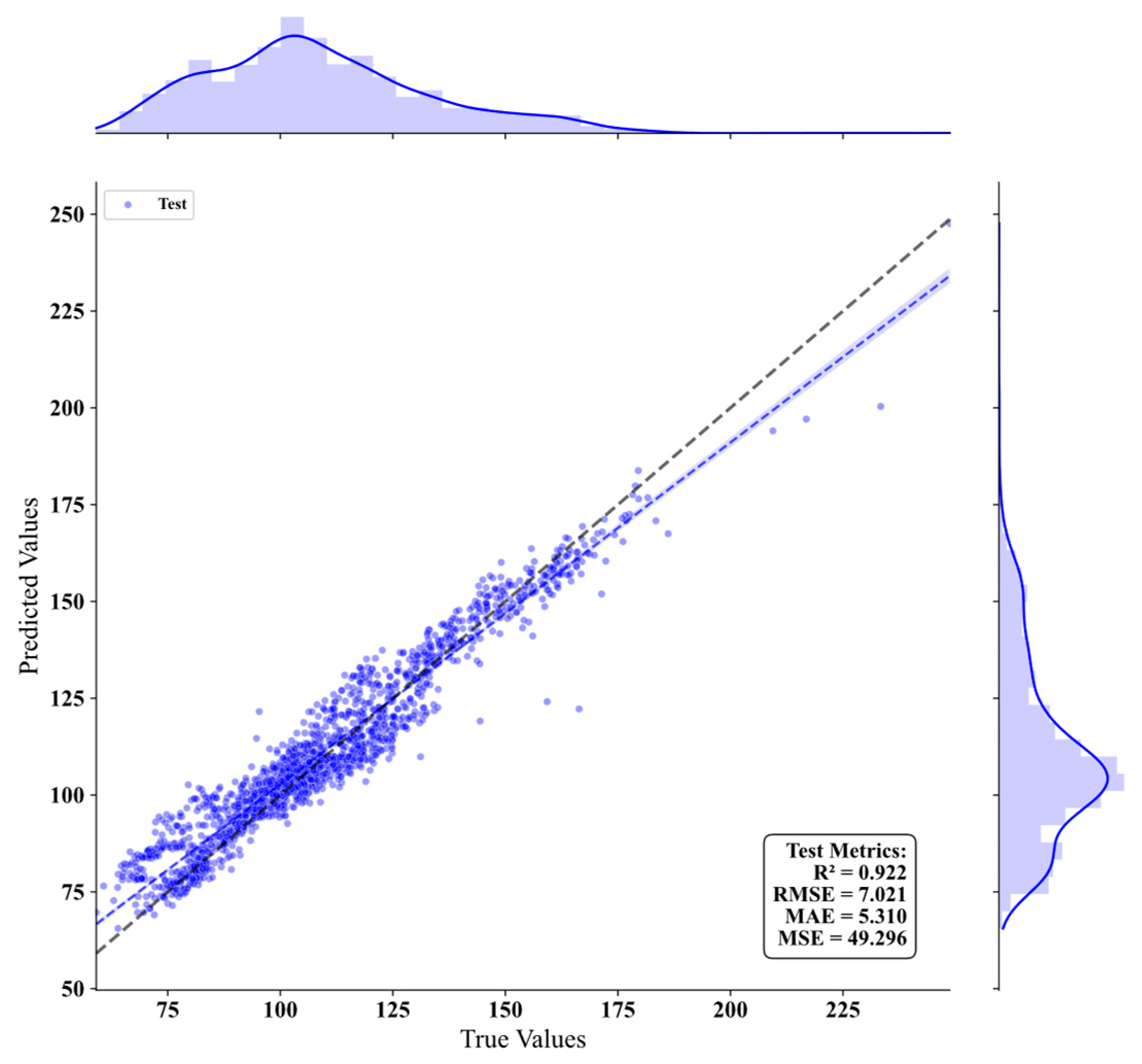
Model Details Analysis: The XGBoost model has the highest R2 value of 0.9217, meaning that this model can explain about 92.2% of the variance, and the model has the lowest MAE and MAPE values of 5.31 and 5.3%, with the smallest and most stable deviation of the predicted value. XGBoost can deal with nonlinear and interactive features well, it has built-in regularization to avoid overfitting, and XGBoost can be a good option for complex data. Multi-Layer Perceptron (MLP) has an R2 value (0.9155) close to XGBoost, but the error is a little more than XGBoost, and it is much less than RF and LR, so MLP can also do a good job of capturing data patterns. MLP is sensitive to data scaling and network structure and may require more parameter tuning or data preprocessing; Random Forest (RF) performs at an average level, with an R2 value (0.8914) similar to LR, but its error metrics, such as MAE and MSE, are higher than LR, possibly due to the presence of many outliers or noise, resulting in large fluctuations in tree models. As an ensemble method, RF is usually robust, but may perform averagely due to data characteristics; Linear Regression (LR) performs the weakest, with the lowest R2 value (0.8912) and the largest errors, indicating that the data may have a significant nonlinear relationship, and LR’s fitting ability is insufficient. LR is simple and has strong interpretability, but if the data does not meet the linear assumption, its performance will naturally be limited.
To demonstrate the predictive power of the optimal model (XGBoost), the scatter plot for the predicted values and actual outcomes on the time-based test dataset is shown in Figure 2. The observations form a closely packed zone around the diagonal with no indication of any bias.
In summary, the process of validation for comparison on the time parameter reaffirms that the XGBoost model outstrips other models with regard to concrete consumption due to the absence of overfitting as the reason for its superior performance. Additionally, the fact that XGBoost is much superior compared to Linear Regression and Random Forest validates its classification as the best predictor for concrete consumption on a daily basis.

4.2. In-Depth Analysis of Influencing Mechanisms Based on SHAP

By applying the SHAP explainable artificial intelligence technique to systematically reveal the action paths, nonlinear characteristics, and interaction mechanisms of various influencing factors on the daily concrete consumption prediction results.

4.2.1. Global Feature Importance Analysis

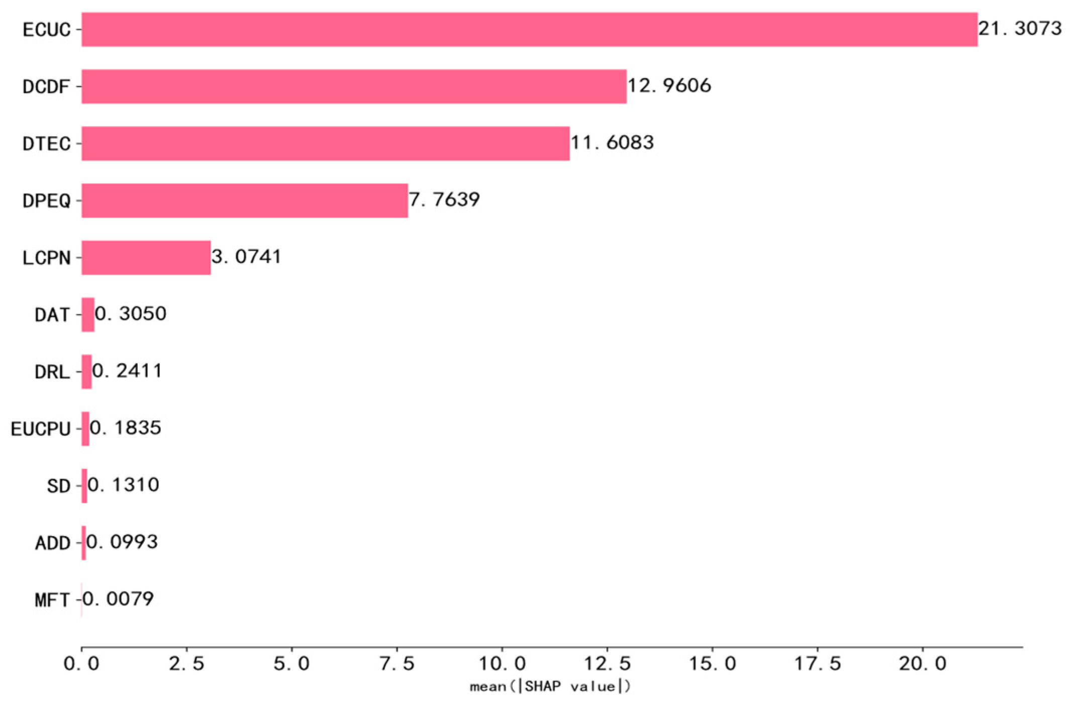
To identify the key drivers influencing the daily consumption of concrete, this study first calculated the mean absolute SHAP value for each feature and ranked them from most to least important, as shown in Figure 3.
Figure 3 shows that Electricity Consumption per Unit Concrete (ECUC) has the highest mean absolute SHAP value at 21.3073, which is the main driving factor leading to the change trend of daily concrete consumption. The daily concrete delivery frequency (DCDF) and the daily total electricity consumption (DTEC) rank second and third in value, at 12.9606 and 11.6083, respectively, establishing them as the main variables that determine the scale of resource allocation. Factors such as the number of times the mixing equipment fails (MFT) and the average delivery delay (ADD) have relatively weak influencing degrees.

4.2.2. Nonlinear Influences and Threshold Effects of Factors

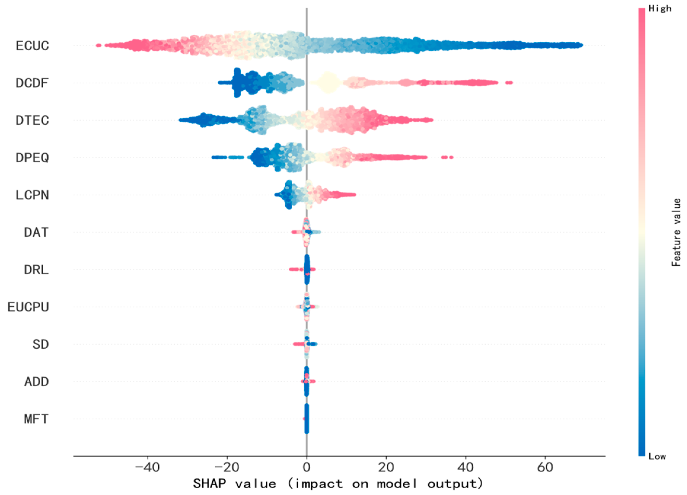
To explore the specific modes of action of key factors on daily concrete consumption in detail, this study further revealed their complex nonlinear relationships and threshold effects through SHAP dependence plots and the beeswarm plot shown in Figure 4.
The study found that there is a significant threshold effect for ECUC. When the value was less than 40.4 kWh/m3, the SHAP values changed gently, indicating a weak inhibitory effect on demand. Once this critical value is exceeded, the SHAP values drop sharply, indicating that too high energy consumption significantly increases resource waste, and the actual usage is far from the reasonable range.
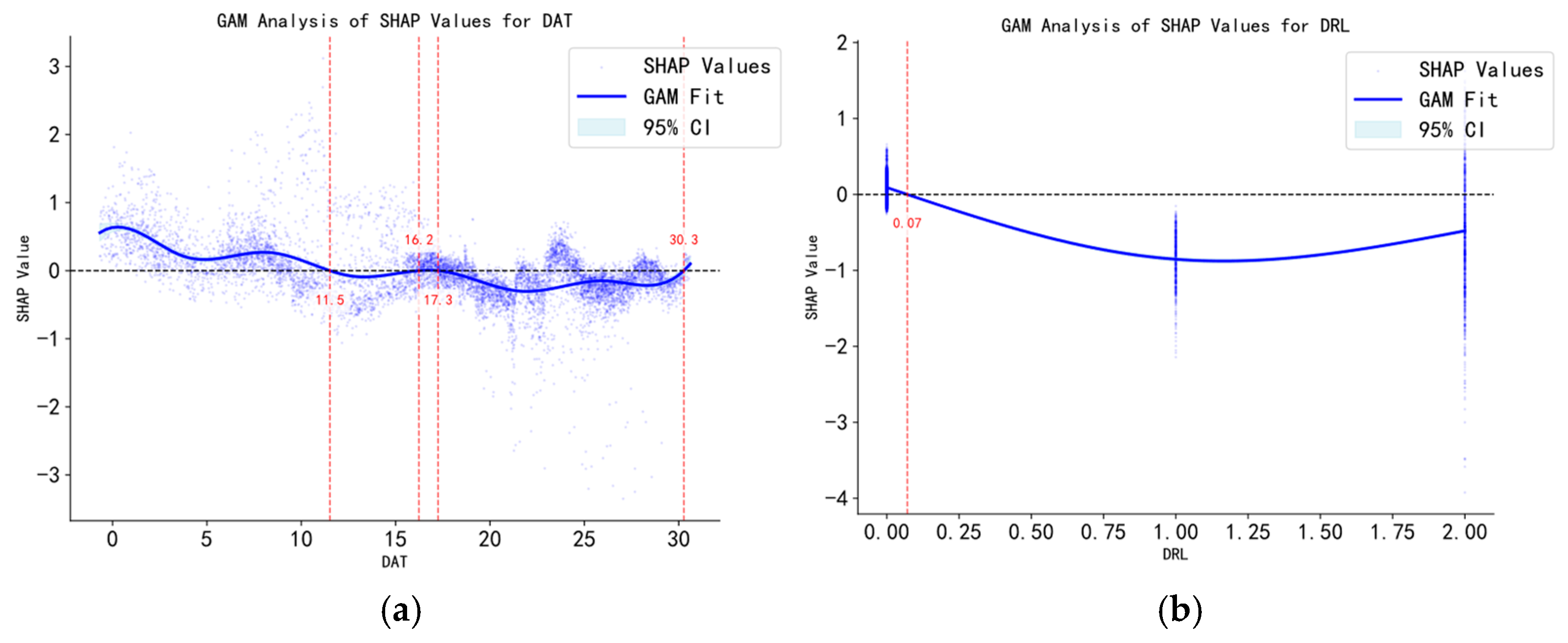
The impact of the environmental factor of daily average temperature (DAT) is segmented behavior. When the temperature is lower than 10.5 °C, the SHAP value is greater than 0, and it is constantly increasing, which indicates that the amount of concrete used will increase with the drop in temperature. From this, it can be inferred that the low-temperature environment will make the concrete construction less efficient. When the temperature is in the range of 10.5–25.3 °C, the SHAP value will change a little, so this is the best temperature impact. When the temperature is larger than 25.3 °C, the SHAP value will be less than 0. Because it is hot, the concrete dries out very fast, and it is used abnormally.
And, also, the effect of Daily Rainfall Level (DRL) was a step-like effect. Its influence was minimal under no-rain conditions, but moderate and heavy rain significantly increased the SHAP value, indicating that heavy rain severely disrupts outdoor construction plans, causing an unexpected increase in demand for concrete.

4.2.3. Analysis of Interaction Effects Between Multiple Factors

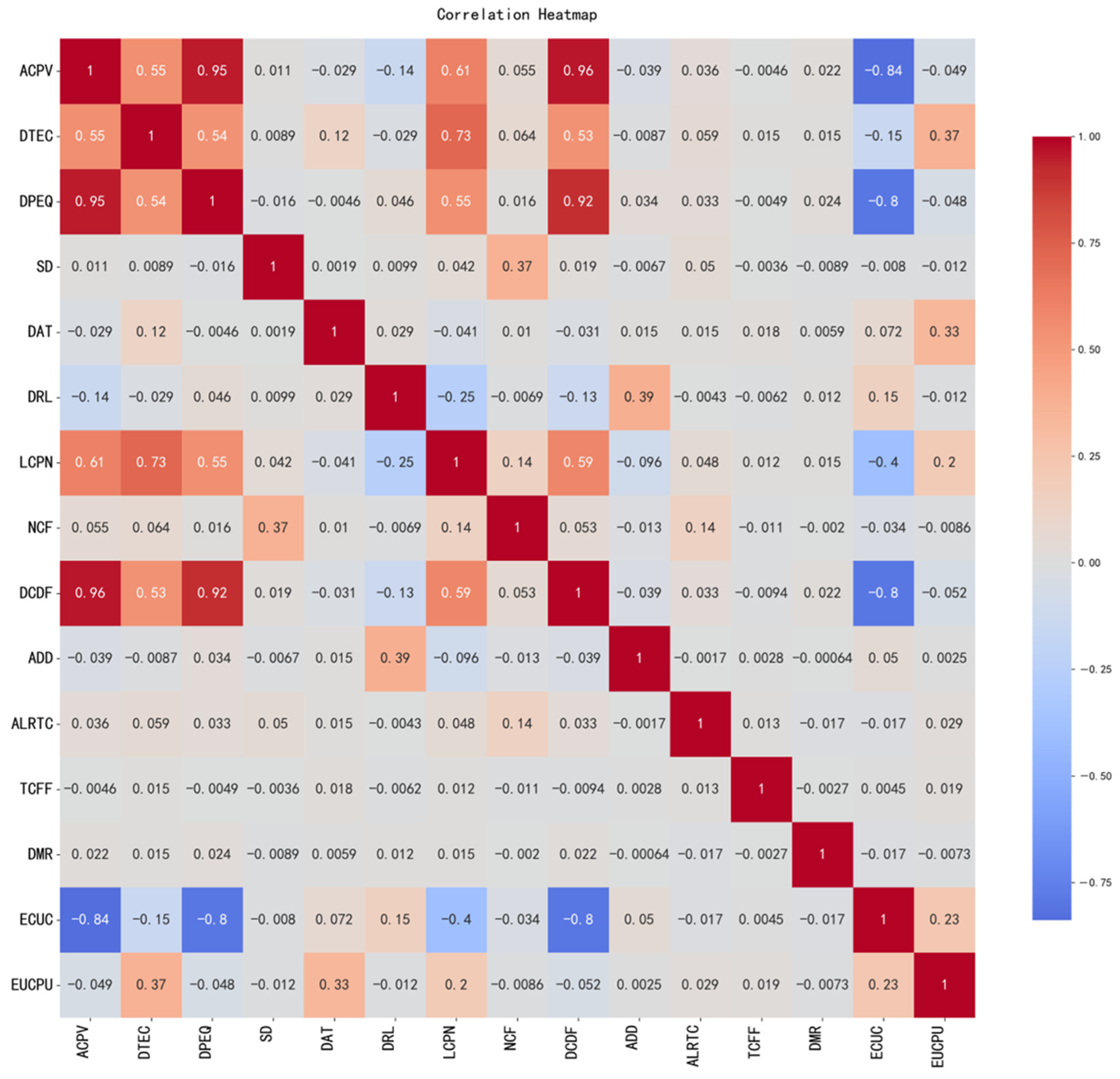
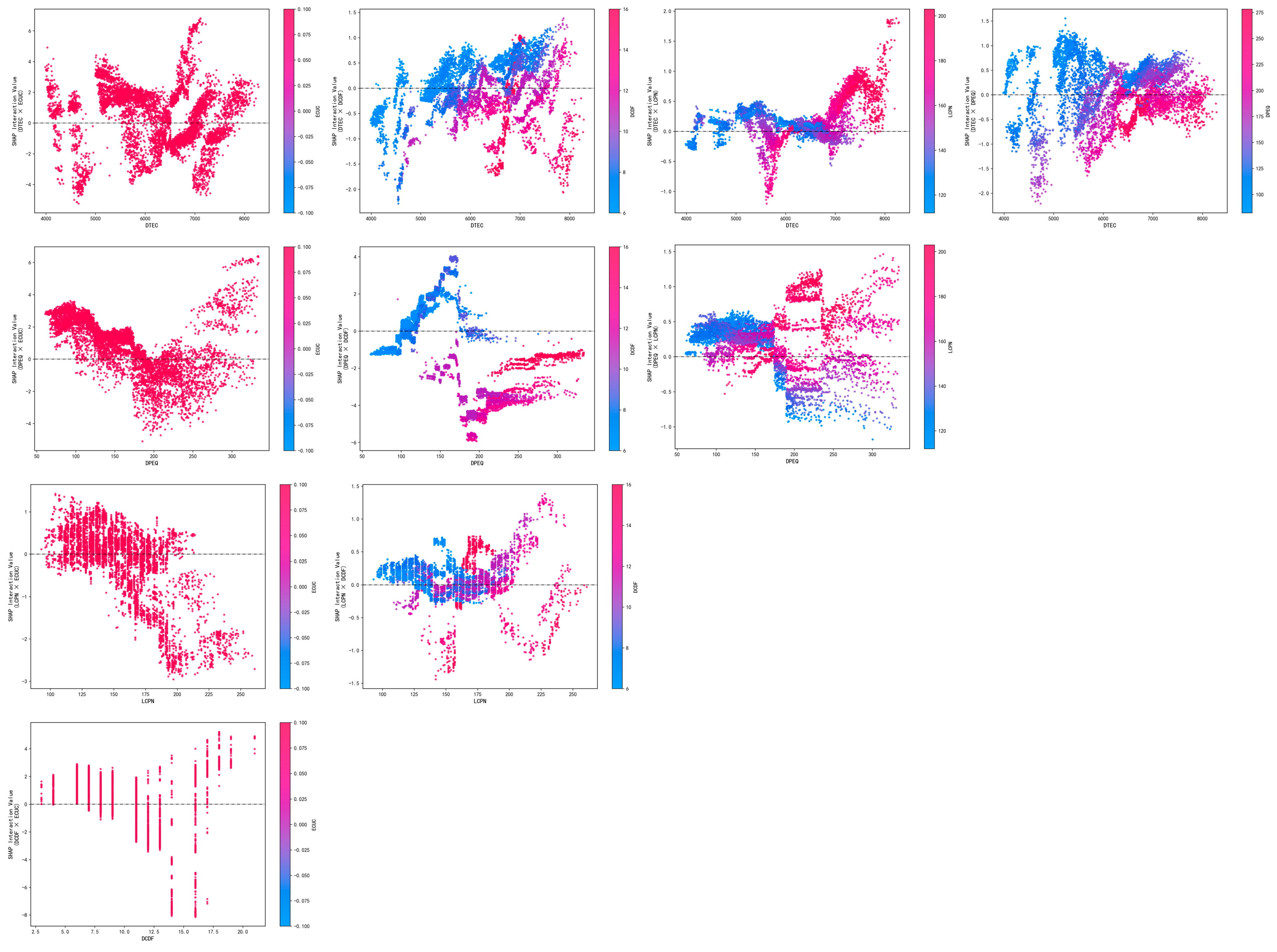
To explore the complex synergistic or antagonistic effects among multiple influencing factors, this study further conducted an interaction effect analysis through SHAP interaction values. The strength matrix of the interaction effects between pairs of main factors is shown in Figure 5. Different colors in the figure represent the degree of impact of the joint on the prediction result for each pair of features. Darker colors indicate a stronger interaction effect for that factor pair.
Figure 5 shows that the darkest color exists between DTEC and DCDF, indicating that the interaction between these two variables is the strongest, which corroborates the conclusions in Section 4.2.2. In addition, ECUC, as the most important single factor, also showed a significant interaction effect with DTEC, suggesting that energy consumption efficiency and overall electricity intensity jointly affect resource demand. To present the key connections in the interaction network more intuitively, an interaction effect network diagram was drawn, as shown in Figure 6.
From the multi-factor interaction analysis, it can be seen that the demand for concrete resources of an infrastructure project is not determined by a single factor, and the demand for concrete resources is a complex network effect of many key driving factors. Identifying them bears a fair amount of instruction for the coordination of control means and precise allocation of resources.
The interaction matrix (Figure 6), besides saying who is stronger than who, also tells us what is happening between each one, which helps us see how the pieces work together at the site. The strongest interaction in DTEC-DCDF indicates the most important synergistic amplification. That is to say, when the construction time is high intensity (DTEC), a concrete delivery has a large impact on the resources of the entire project. This is an example of energy intensity and supply chain rhythm. An activity like slip form construction, a peak activity, might be producing a lot of waste because there are a lot of trucks that are lined up, or it may have a lot of equipment that is sitting idling, and so the delivery is not matched with the high-energy activity.
This is the basic reasoning to obtain the dynamic matching coefficient K = DCDF/DPEQ in the planning and execution coordination layer. A key managerial lesson is that schedules cannot be optimized without live energy profiles. The K coefficient is like a lever that is grabbing onto this synergy and making sure that all of the materials that are floating around are keeping up with the energy of the project; instead of everything going wrong, it turns into a moment to get better at working together.
Also, we can observe that less interaction of environmental factors, such as DAT with other factors, indicates that even if the environment is changing, the most important thing to consider is the cooperation between energy and logistics. This hierarchy of interaction tells us which interactions need the most effort into their management, because we can see that energy and supply chains will have to be given the highest level of priority, as these are the pairs that have the most influence in preventing a nonlinear escalation of resources.

4.3. Hierarchical Optimization Strategy for Concrete Resources

Based on the SHAP analysis results, this study constructs a three-level optimization system to provide hierarchical and operational decision support for the precise management of specific resources. This system divides the optimization strategies into the “Core Process Monitoring Layer”, the “Planning and Execution Coordination Layer”, and the “External Environment Adaptation Layer” according to the timeliness of management intervention, the controllability of factors, and the complexity of the path of impact. The framework is intended to provide specific, measurable, and stratified decision-making support for the management of concrete resources, and to promote the transformation of project management from experience-based practices to a dual-driven model of data and mechanism.

4.3.1. Core Process Monitoring Layer

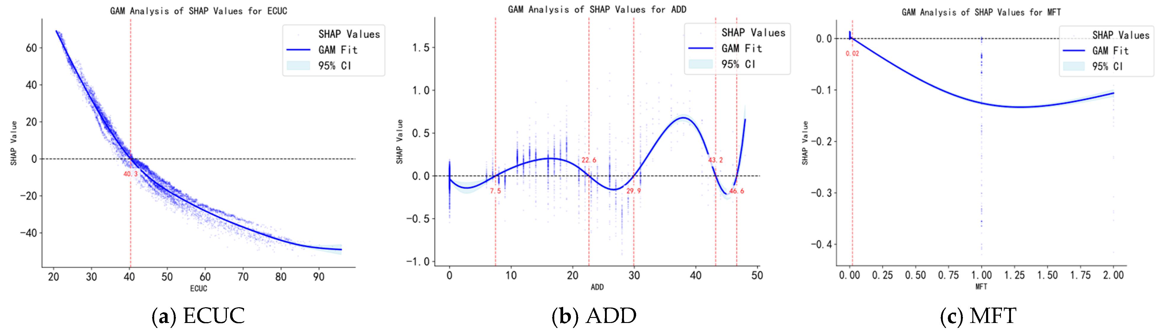
This layer is about the core process indicators that will affect the use of the resources on the day of construction. It sets up an immediate response method of “pre-event warning, in-process control”, real-time monitoring, and quantity threshold control. The SHAP dependence analysis and GAM analysis prove that there are important nonlinear turning points in factors such as ECUC, and add, as well as the MFT analysis, which offer scientific support for management.
Figure 7 reveals the nonlinear relationship between core process factors and concrete consumption through the Generalized Additive Model (GAM). The shaded area around the smooth curve in the figure represents the confidence interval of the fit, and the change in the slope of the curve intuitively reflects the intensity variation in the factor’s influence. When the ECUC is less than 40.3 kWh/m3, the negative impact of its excessive consumption on concrete is within the controllable range. However, once this threshold is exceeded, the SHAP value drops sharply, indicating a nonlinear, steep rise in the risk of resource waste. This nonlinear feature indicates that high energy consumption is not only a sign of low equipment efficiency, but also a strong signal of blockage in the construction process.
So, from this research, it shows that the main performance level of the project’s energy efficiency control is at 40.3 kWh/m3. Use the IoT system to record and calculate the ECUC value. Once the measured value continues to exceed the upper limit, the management system will automatically sound the alarm. This alert should be dealt with to conduct a root cause analysis and change the operational state of the equipment and the smoothness of the construction process as soon as possible, so that the efficiency loss and resource waste will not occur from the source.
And, similar to ADD and MFT, nonlinear effects emerge. When ADD is above around 29.9 min or MFT freq becomes unnaturally high, these circumstances would cause the effect on maintaining the continuous construction progress and the efficiency of the resource distribution to become even more evident. So, we need an amber warning for the supply chain and the state of equipment. The tolerance will depend on a few things. When multiple indicators are all abnormal, we should perform the collaborative diagnosis and correction of multiple indicators at the same time, so that local problems will not gradually become a comprehensive efficiency bottleneck.
To sum up, through the core process monitoring layer, data insights are converted into quantified action thresholds, and site management moves from subjective experience judgment to objective data-based decision-making. This layer provides strong real-time data support and immediate intervention ability for the entire optimization system, and an intervention path can be drawn.

4.3.2. Planning and Execution Coordination Layer

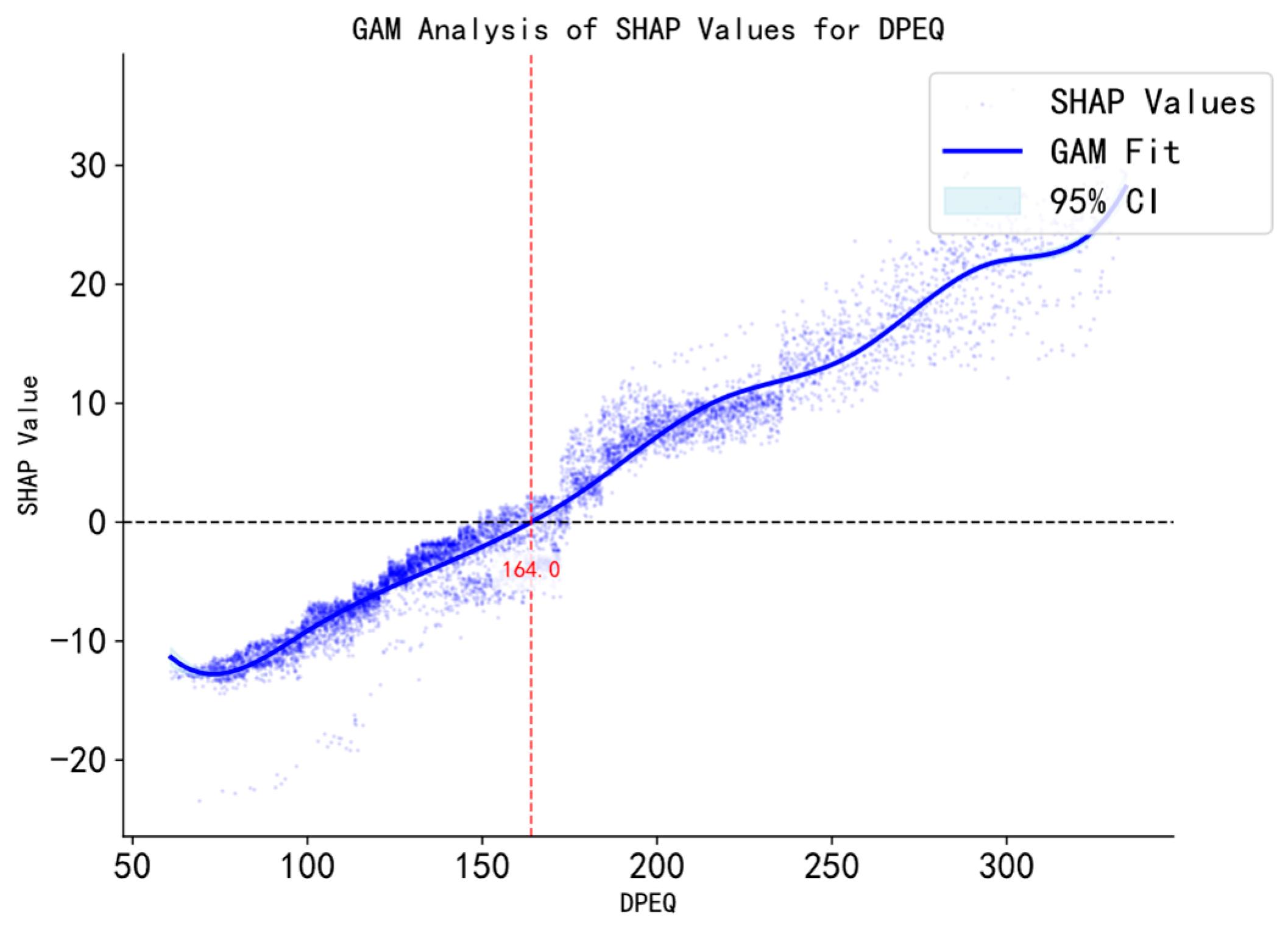
This layer solves the problem of dynamic adjustment between “planning” and “execution” in the construction process and aims to overcome the contradiction of resource excess or shortage caused by rigid planning. SHAP interaction analysis shows that there is a significant synergistic effect rather than a simple linear superposition between Daily Planned Engineering Quantity (DPEQ) and Daily Concrete Delivery Frequency (DCDF). This interaction mechanism is one of the important causes of the phenomenon of resource matching between farmers and capital.
Figure 8 clearly demonstrates the synergistic amplification effect between planned engineering quantity (DPEQ) and concrete delivery frequency (DCDF) through the GAM interaction surface. When DPEQ is below 164 m3, the surface remains relatively flat (Z-axis variation ≤ 5%), indicating that increasing the delivery frequency has a limited impact on consumption. However, when DPEQ reaches or exceeds 164 m3, the surface shows a significant steep rise (Z-axis variation ranging from 12% to 18%), revealing that during high-intensity construction phases, it is crucial to coordinate the ratio between these two variables. It is recommended to establish a dynamic matching coefficient K = DCDF/DPEQ. When the K value deviates from the optimal interval [0.08, 0.12], an automatic scheduling adjustment should be triggered to achieve fine-grained management linked to plannin–execution.
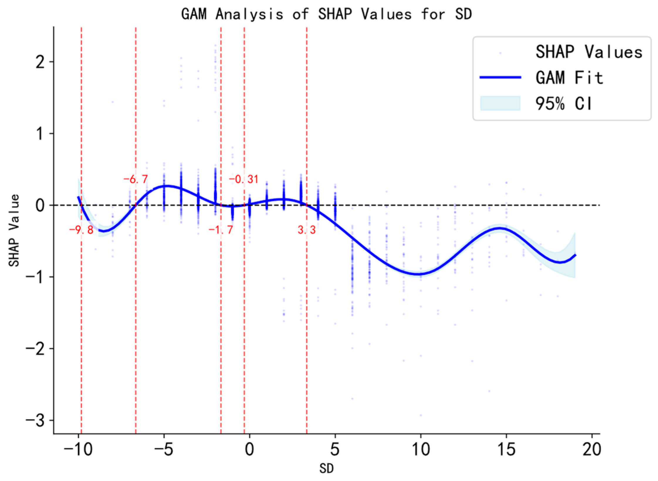
Figure 9 shows a typical S-curve for the GAM analysis for Schedule Deviation (SD). As SD is within the range of ±5%, the SHAP values vary by less than 1.5 on the SHAP value axis and form a flat curve (almost horizontal), which means that normal tweaking is needed for resource stability at this stage. Above the range of ±5%, the rate at which the SHAP values rise is more substantial (between 3.2 and 4.5 values on the SHAP value axis map), which implies the activation of a graded response system. For deviations between 5% and 10%, there is a need for adjusting the frequency rates, and above 10% deviations require simultaneous resource allocation for proper management. When a deviation occurs, an automatic resource reallocation algorithm will be triggered. This algorithm incorporates the interaction between DPEQ and DCDF identified in the model with the trend of the SD itself to achieve rolling prediction and calibration of the daily concrete pouring volume required.
At the same time, the mechanism synchronously optimizes labor shifts and equipment deployment scale to achieve the coordinated management of “Man–Machine–Material”. For example, if the forecasted workload increases due to accelerated progress, the system prompts an increase in DCDF and adds more people. On the other hand, if the progress is behind, it will notify the supply chain to reduce the number of deliveries to avoid equipment idling or material waste caused by premature setting of the concrete.
In addition, the strategy provides for flexible time-window management. This replaces fixed delivery schedules with optimized and adaptable time intervals that are in line with the core operating hours and dynamically adjusted according to the SD. This adjustment avoids disruption of supply chains and unloading conflicts due to sudden changes in the plan.
To sum up, this strategy transforms the findings of the SHAP analysis into an adaptive management tool. Promotes the transformation of resource scheduling from “periodic adjustment after the fact” to “real-time dynamic optimization”, and provides an important way to achieve the precise matching of resource supply and demand. Strategic transformation of the surrounding “three areas” to enhance the overall regional competitiveness.

4.3.3. External Environment Adaptation Layer

This layer addresses the disruptions caused by uncontrollable external environmental factors in concrete construction and resource scheduling, such as ambient temperature and rainfall. It is expected to transform the traditional experience—dependent, reactive response mode into a data-driven and precise dynamic management system.
Figure 10 quantifies the concept of a ‘comfort zone’ for environmental factors through GAM analysis. Regarding temperature, within the range of 10.5–25.3 °C, the SHAP value fluctuation is less than 0.8 (indicating a flat segment of the curve), which can be considered a stable zone for construction efficiency. However, when the temperature falls below the lower limit of 10.5 °C or exceeds the upper limit of 25.3 °C, the SHAP values show significant deviations of +2.1 and −3.4, respectively. Based on these findings, it is recommended to use early-strength agent formulations during low-temperature periods, increase the frequency of curing during high-temperature periods, and set a rainfall intensity greater than 10 mm/day as a trigger condition for dynamic plan adjustments.
To put it briefly, the External Environment Adaptation Layer takes the environmental impact mechanism that we found out through the SHAP analysis and turns it into real, numerical management standards and coping methods. And it has made a big leap from the experience of judging to making scientific decisions, and it is also a part that can ensure that the specific resources are in precise control, and the progress of the project can be carried out smoothly.

5. Discussion

5.1. Main Findings

5.1.1. Synergistic Effect of the XGBoost-SHAP Framework

The XGBoost model in this paper has a good effect on the time-series test set, with an R2 of 0.922, which is much better than the baseline models such as linear regression and Random Forest [37] on the time-series test set with an R2 of 0.922. The results demonstrate the inherent advantages of these ensemble learning algorithms for tackling the high-dimensional and nonlinear data from construction engineering fields, and a means for explaining structural limits of linear models in showing dynamic interactions between a large number of factors at construction sites [38,39]. While XGBoost is highly effective at identifying complex correlations between variables (e.g., engineering volume and delivery frequency), it does not inherently provide the interpretable insights needed to directly empower management decisions.The most important finding of this paper is that we successfully opened the “black box” of the prediction model by using the SHAP interpretable model. SHAP analysis can not only give the global importance of each feature to the prediction result [40,41], but also some drivers, such as the unit concrete electricity consumption ECUC with nonmonotonic and nonlinear effects. The fact that, for example, ECUC suddenly turns its direction is not a flaw in the model but is a correct representation of the construction’s energy efficiency. It is a very precise prediction and a very clear explanation. That is the greatest achievement of the method of this study; this study changes resource regulation from being far behind to taking resource regulation as an empirical guess.

5.1.2. Key Driving Mechanisms

The most important feature, according to SHAP analysis, is unit concrete electricity consumption (ECUC). Consequently, this oversight has significant implications for engineering management. The core issue lies in the failure to analyze the project from an ECUC (Energy Consumption per Unit of Construction) perspective, which serves as the most critical indicator of energy efficiency. As a primary representative of the entire construction process, ECUC effectively reflects the systemic synergy among equipment, schedule, and workflow. Specifically, an ECUC value below 40.3 kWh/m3 signifies a cooperative and efficient state among these factors. Conversely, when ECUC exceeds 42 kWh/m3, it indicates underlying pathologies: the equipment is likely outdated, the process is plagued by conflicts, and the schedule is overly rigid. This inefficient state leads to a sharp decrease in marginal energy productivity and a nonlinear increase in the risk of resource misallocation. Further, it is the red line of the construction energy efficiency’s health, and it can provide a precise and numerical standard for the real-time supervision and early warning on site [42]. By establishing environmental sensitivity thresholds (e.g., a comfortable daily average temperature range of 10.5–25.3 °C), uncontrollable external factors become predictable and manageable; Beyond this range, construction efficiency losses due to low temperatures and concrete workability reduction due to high temperatures can trigger significant nonlinear variations in resource consumption.It asks the project manager to become less of a passive recipient of the weather and more of an active user of climate windows and to make a different construction organization plan [43]. Moreover, there are some multi-factor interaction effects that are highly synergistic, such as DTEC-DCDF, the interaction between total daily electricity consumption and delivery frequency, implying that the demand on the resource is an endogenous of the system. Managing only one variable, or a variable, or any variable, by itself or independently will be weak as a result of ignoring the system synergies.

5.1.3. Hierarchical Optimization Strategies Transformation Path

This article does not desire an absolutely perfect predictive model. Instead, it uses this model to actively and efficiently manage. According to the threshold and the interaction of the SHAP, we design a 3-level improvement plan: control of key processes, coordination of plan execution, and change of external environment. The innovation of this strategy system is the creation of a pathway to change data insight into management decisions [44]. Core process monitoring layer transforms the core mechanism indicators, such as ECUC threshold, into an active intervention during the process itself, even before, from a passive after-the-fact reaction. For the planning execution coordination layer, grasp the interaction of DPEQ and DCDF, and realize the transformation from macro-planning to micro-execution through the dynamic coefficient K = DCDF/DPEQ. Historical problem of “changes behind plans”. The External Environment Adaptation Layer makes DAT’s comfort zone become a basis of construction organization adjustment, which leaped from “tolerance” to “adaptation” in the external environment.
This hierarchy design’s key point is to break down the unified, comprehensive model prediction results into specific, detailed tasks that managers at every level (project managers, dispatchers, team leaders, etc.) can recognize and act on from the “last mile” gap between an algorithm’s prediction result and real-life on-site action.

5.2. Theoretical Implications

Combined with XGBoost, SHAP, and GAM, and establishing a complete technical system framework, it is possible to provide a full research paradigm for construction engineering management studies with high precision prediction, mechanism explanation, and strategic design. The uncovered nonlinear threshold impact and interaction phenomenon are different from the old linear model and static thought. It provides a new theoretical viewpoint to handle intricate engineering systems, giving both a microscopic mechanical explanation and a method for realizing the prediction-decision integration concept. It drives paradigm change from single-parameter optimization to synergy systems with regard to engineering management theories, and it bridges the gap between current prediction analysis and managerial knowledge.

5.3. Practical Implications

In reality, a hierarchy optimization strategy system centers on planning and coordinating, where the environment is appropriate for operationalizing the data-driven insights. For example, maybe the senior decision makers will use something global like ECUC for the top control level. And then you have your on-site managers, and they are going to be wanting to get a little bit dirtier and get a daily breakdown of features and SHAP values so that they can understand what they need to be scheduling. And it gets us out of the business of what we used to do and moves us into something that is a lot more precise and mechanical. And this is how it is going be used, so being able to watch the ECUC threshold in real time is going to be in your daily routine and the DPEQ plus DCDF is for the weekly routine when you want to purchase to avoid too little and too much, and then changing to fit DAT is good for when it is super hot or super cold outside. It provides a clear, practical guide for applying research findings, as well as a tangible roadmap for digitally transforming building resource management.

6. Conclusions

This study demonstrates that the XGBoost-SHAP framework can accurately predict the consumption of concrete with a high precision (R2 = 0.922), and has identified the systematic driving factors such as nonlinear thresholds and factor interaction. And making all those observations into layers of optimizations, the research has provided a kind of technical class that can utilize resources more efficiently—this is superior to the previous approach of relying solely on experience and guesswork.
Theoretically, this study offers a new paradigm for understanding the complex decision-making process in engineering management by introducing the explainable artificial intelligence framework, promoting the transformation of static linear thinking to dynamic systematic thinking. In practice, the research results provide an accurate decision support framework for managers at all levels of the project, whether for macro-strategic control or micro-daily scheduling, and present a feasible and high-usability implementation plan for the digital transformation of engineering management.
However, this study has some limitations. Despite having such a strong backend framework for analysis, in order to make this adoption model more widely promoted among construction managers who do not possess the specific skills and knowledge required for backend analysis, integration with a friendly interface would be necessary and would ensure that a purely backend solution for analysis is not a hindrance to adoption. A significant direction for research would therefore be integration with a friendly interface. Future research could integrate BIM, real-time data from IoT sensors, and market fluctuation information to develop a more forward-looking and adaptable digital twin analysis system. Secondly, regarding model generality, while the framework has been validated for effectiveness in large-scale landmark infrastructure, its applicability across a broader range of engineering types requires further cross-domain comparative verification and adaptive optimization. Finally, for application transformation, this is the current model, which is a backend analysis model and needs some knowledge to operate. The most actionable next step would be to create a lightweight DSS that can be integrated with the main algorithms of this research study, with a GUI and an early warning dashboard for key indicators, so that the frontline project manager can use the research results easily and intuitively, thereby achieving a good transformation from academic innovation to industrialization.

Author Contributions

Conceptualization, R.Z. and Y.G.; methodology, R.Z.; software, Y.G.; validation, X.L.; formal analysis, Y.G.; investigation, Y.G. and X.L.; data curation, X.L.; writing—original draft preparation, Y.G.; writing—review and editing, R.Z.; visualization, X.L.; supervision, R.Z.; project administration, R.Z. All authors have read and agreed to the published version of the manuscript.

Funding

This research was funded by the Humanities and Social Sciences Foundation of Ministry of Education of China (No. 24YJC630298), the National Natural Science Foundation of China (NSFC) (No. 71801119), the Basic Research Project of the Education Department of Liaoning Province (No. LJ112510147006), and the Research Project on the Economic and Social Development of Liaoning Province (No. 2026lslybwzzkt-025).

Data Availability Statement

The original contributions presented in this study are included in the article. Further inquiries can be directed to the corresponding author.

Conflicts of Interest

The authors declare no conflicts of interest.

References

  1. Al-Aloosy, K.F.Q.; Mirvalad, S.; Shabakhty, N. Evaluating the impact of internet communication quality in human resource management on the productivity of construction projects. Heliyon 2024, 10, e28500. [Google Scholar] [CrossRef]
  2. Rasanjali, W.A.; Mendis, A.P.K.D.; Perera, B.A.K.S.; Disaratna, V. Implementing enterprise resource planning for lean waste minimisation: Challenges and proposed strategies. Smart Sustain. Built Environ. 2024, 13, 330–353. [Google Scholar] [CrossRef]
  3. Zhang, N.; Konyaloglu, A.K.; Duan, H.; Feng, H.; Li, H. The impact of innovative technologies in construction activities on concrete debris recycling in China: A system dynamics-based analysis. Environ. Dev. Sustain. 2023, 26, 14039–14064. [Google Scholar] [CrossRef]
  4. Cheng, J.; Tegge, A.N.; Baldi, P. Machine learning methods for protein structure prediction. IEEE Rev. Biomed. Eng. 2008, 1, 41–49. [Google Scholar] [CrossRef] [PubMed]
  5. Chitkeshwar, A. Revolutionizing structural engineering: Applications of machine learning for enhanced performance and safety. Arch. Comput. Methods Eng. 2024, 31, 4617–4632. [Google Scholar] [CrossRef]
  6. Ma, T.; Chen, H.; Zhang, K.; Shen, L.; Sun, H. The rheological intelligent constitutive model of debris flow: A new paradigm for integrating mechanics mechanisms with data-driven approaches by combining data mapping and deep learning. Expert Syst. Appl. 2025, 269, 126405. [Google Scholar] [CrossRef]
  7. Shen, L.; Ma, T.; Chen, H.; Ye, B.; Luo, R.; Sun, H. A new CNN-GRU deep learning framework optimized by CHIO for precise prediction of debris flow velocity. Stoch. Environ. Res. Risk Assess. 2025, 39, 2351–2371. [Google Scholar] [CrossRef]
  8. Hamilton, R.I.; Papadopoulos, P.N. Using SHAP Values and Machine Learning to Understand Trends in the Transient Stability Limit. IEEE Trans. Power Syst. 2023, 39, 1384–1397. [Google Scholar] [CrossRef]
  9. Othman, I.; Napiah, M.; Potty, N.S. Resource management in construction project. In Applied Mechanics and Materials; Trans Tech Publications Ltd.: Baech, Switzerland, 2014; Volume 567, pp. 607–612. [Google Scholar] [CrossRef]
  10. Chen, Q.; García de Soto, B.; Adey, B.T. Construction automation: Research areas, industry concerns and suggestions for advancement. Autom. Constr. 2018, 94, 22–38. [Google Scholar] [CrossRef]
  11. Lee, J.S.; Ham, Y.; Pork, H.; Kim, J. Challenges, tasks, and opportunities in teleoperation of excavator toward human-in-the-loop construction automation. Autom. Constr. 2022, 135, 104119. [Google Scholar] [CrossRef]
  12. Li, L.; Luan, H.; Yin, X.; Dou, Y.; Yuan, M.; Li, Z. Understanding Sustainability in Off-Site Construction Management: State of the Art and Future Directions. J. Constr. Eng. Manag. 2022, 148, 03122008. [Google Scholar] [CrossRef]
  13. Gurgun, A.P.; Koç, K.; Kunkcu, H. Exploring the adoption of technology against delays in construction projects. Eng. Constr. Archit. Manag. 2024, 31, 1222–1253. [Google Scholar] [CrossRef]
  14. Li, X.; Lu, W.; Xue, F.; Wu, L.; Zhao, R.; Lou, J.; Xu, J. Blockchain-Enabled IoT-BIM Platform for Supply Chain Management in Modular Construction. J. Constr. Eng. Manag. 2021, 148, 04021195. [Google Scholar] [CrossRef]
  15. Wang, X.; Mazumder, R.K.; Salarieh, B.; Salman, A.M.; Shafieezadeh, A.; Li, Y. Machine Learning for Risk and Resilience Assessment in Structural Engineering: Progress and Future Trends. J. Struct. Eng. 2022, 148, 03122003. [Google Scholar] [CrossRef]
  16. Fayek, A.R. Fuzzy Logic and Fuzzy Hybrid Techniques for Construction Engineering and Management. J. Constr. Eng. Manag. 2020, 146, 04020064. [Google Scholar] [CrossRef]
  17. Liu, L.; Hodgins, J. Learning basketball dribbling skills using trajectory optimization and deep reinforcement learning. ACM Trans. Graph. 2018, 37, 142. [Google Scholar] [CrossRef]
  18. Wang, X.; El-Gohary, N. Deep learning-based relation extraction and knowledge graph-based representation of construction safety requirements. Autom. Constr. 2023, 147, 104696. [Google Scholar] [CrossRef]
  19. Parsamehr, M.; Perera, U.S.; Dodanwala, T.C.; Perera, P.; Ruparathna, R. A review of construction management challenges and BIM-based solutions: Perspectives from the schedule, cost, quality, and safety management. Asian J. Civ. Eng. 2023, 24, 353–389. [Google Scholar] [CrossRef]
  20. Li, Z.; Lei, H.; Ma, E.; Lei, J.; Qu, J. Ensemble technique to predict post-earthquake damage of buildings integrating tree-based models and tabular neural networks. Comput. Struct. 2023, 269, 107114. [Google Scholar] [CrossRef]
  21. Zhang, J.; Yuan, J.; Mahmoudi, A.; Ji, W.; Fang, Q. A data-driven framework for conceptual cost estimation of infrastructure projects using XGBoost and Bayesian optimization. Constr. Manag. 2024, 24, 751–774. [Google Scholar] [CrossRef]
  22. Lyngdoh, G.A.; Zaki, M.; Krishnan, N.M.A.; Das, S. Prediction of concrete strengths enabled by missing data imputation and interpretable machine learning. Cem. Concr. Compos. 2022, 128, 104414. [Google Scholar] [CrossRef]
  23. Shehadeh, A.; Alshboul, O.; Almalki, R.E.A.; Homedat, O. Machine learning models for predicting the residual value of heavy construction equipment: An evaluation of modified decision tree, LightGBM, and XGBoost regression. Autom. Constr. 2021, 129, 103827. [Google Scholar] [CrossRef]
  24. Wu, Y.; Cai, D.; Gu, S.; Jiang, N.; Li, S. Compressive strength prediction of sleeve grouting materials in prefabricated structures using hybrid optimized XGBoost models. Constr. Build. Mater. 2025, 476, 141319. [Google Scholar] [CrossRef]
  25. Guan, D.; Shi, Y.; Zhou, L.; Zhu, X.; Zhao, D.; Peng, G.; He, X. Construction and Application of Carbon Emissions Estimation Model for China Based on Gradient Boosting Algorithm. Remote Sens. 2025, 17, 2383. [Google Scholar] [CrossRef]
  26. Chamola, V.; Hassija, V.; Sulthana, A.R.; Ghosh, D.; Dhingra, D.; Sikdar, B. A review of trustworthy and explainable artificial intelligence. IEEE Access 2023, 11, 78994–79015. [Google Scholar] [CrossRef]
  27. Khan, N.; Coleri, S.; Abdallah, A.; Celik, A.; Eltawil, A.M. Explainable and robust artificial intelligence for trustworthy resource management in 6G networks. IEEE Commun. Mag. 2024, 62, 50–56. [Google Scholar] [CrossRef]
  28. Liu, B.; Liu, P.; Lu, W.; Olofsson, T. Explainable artificial intelligence (XAI)for material design and engineering applications: A quantitative computational framework. Int. J. Mech. Syst. Dyn. 2025, 5, 236–265. [Google Scholar] [CrossRef]
  29. Amangeldy, B.; Imankulov, T.; Tasmurzaev, N.; Dikhanbayeva, G.; Nurakhov, Y. A review of artificial intelligence and deep learning approaches for resource management in smart buildings. Buildings 2025, 15, 2631. [Google Scholar] [CrossRef]
  30. Senevirathna, T.; La, V.H.; Marcha, S.; Siniarski, B.; Liyanage, M.; Wang, S. A survey on XAI for 5G and beyond security: Technical aspects, challenges and research directions. IEEE Commun. Surv. Tutor. 2025, 27, 941–973. [Google Scholar] [CrossRef]
  31. Thapa, I.; Ghani, S.; Paramasivam, P.; Tufa, M.A. Development of an optimized deep learning model for predicting slope stability in nano silica stabilized soils. Sci. Rep. 2025, 15, 26213. [Google Scholar] [CrossRef]
  32. Rady, M.; Soliman, A. Performance of fiber-reinforced ultra-high-performance concrete incorporated with microencapsulated phase change materials. Fibers 2023, 11, 94. [Google Scholar] [CrossRef]
  33. Zhai, X. Integrated Planning and Scheduling for Precast Concrete Production. Doctoral Dissertation, Nanyang Technological University, Singapore, 2007. [Google Scholar]
  34. Amjad, M.A.; Sigurdur, E.; Leif, S.; Englund, C. Predicting pavement condition index using an ML approach for a municipal street network. J. Transp. Eng. Part B: Pavements 2025, 151, 04025025. [Google Scholar] [CrossRef]
  35. Hooshyar, D.; Yang, Y. Problems with SHAP and LIME in interpretable AI for education: A comparative study of post-hoc explanations and neural-symbolic rule extraction. IEEE Access 2024, 12, 137472–137490. [Google Scholar] [CrossRef]
  36. Das, P.; Kashem, A.; Hasan, I.; Islam, M. A comparative study of machine learning models for construction costs prediction with natural gradient boosting algorithm and SHAP analysis. Asian J. Civ. Eng. 2024, 25, 3301–3316. [Google Scholar] [CrossRef]
  37. Qin, Y.; Song, D.J.; Chen, H.F.; Cheng, W.; Jiang, G.; Cottrell, G.W. A dual-stage attention-based recurrent neural network for time series prediction. In Proceedings of the 26th International Joint Conference on Artificial Intelligence, Melbourne, Australia, 19–25 August 2017; pp. 2627–2633. [Google Scholar] [CrossRef]
  38. Ouyang, F.; Wu, M.; Zheng, L.Y.; Zhang, L.; Jiao, P. Integration of artificial intelligence performance prediction and learning analytics to improve student learning in online engineering course. Int. J. Educ. Technol. High. Educ. 2023, 20, 4. [Google Scholar] [CrossRef]
  39. Love, P.E.; Irani, Z.; Edwards, D.J. A rework reduction model for construction projects. IEEE Trans. Eng. Manag. 2004, 51, 426–440. [Google Scholar] [CrossRef]
  40. George, S.V.; Kachhara, S.; Ambika, G. Early warning signals for critical transitions in complex systems. Phys. Scr. 2023, 98, 072002. [Google Scholar] [CrossRef]
  41. Wei, H.; Horns, P.; Sears, S.F.; Huang, K.; Smith, C.M.; Wei, T.L. A systematic meta-review of systematic reviews about interprofessional collaboration: Facilitators, barriers, and outcomes. J. Interprof. Care 2022, 36, 735–749. [Google Scholar] [CrossRef] [PubMed]
  42. Pan, Y.; Zhang, L.M. Roles of artificial intelligence in construction engineering and management: A critical review and future trends. Autom. Constr. 2021, 122, 103517. [Google Scholar] [CrossRef]
  43. Gong, D.; Hu, M.; Yin, Y.; Zhao, T.; Ding, T.; Meng, F.; Xu, Y.; Chen, Y. Practical application of artificial intelligence technology in glaucoma diagnosis. J. Ophthalmol. 2022, 2022, 5212128. [Google Scholar] [CrossRef]
  44. Li, Z.R.; Hu, J.; Leng, B.; Xiong, L.; Fu, Z. An integrated of decision making and motion planning framework for enhanced oscillation-free capability. IEEE Trans. Intell. Veh. 2024, 25, 5718–5732. [Google Scholar] [CrossRef]
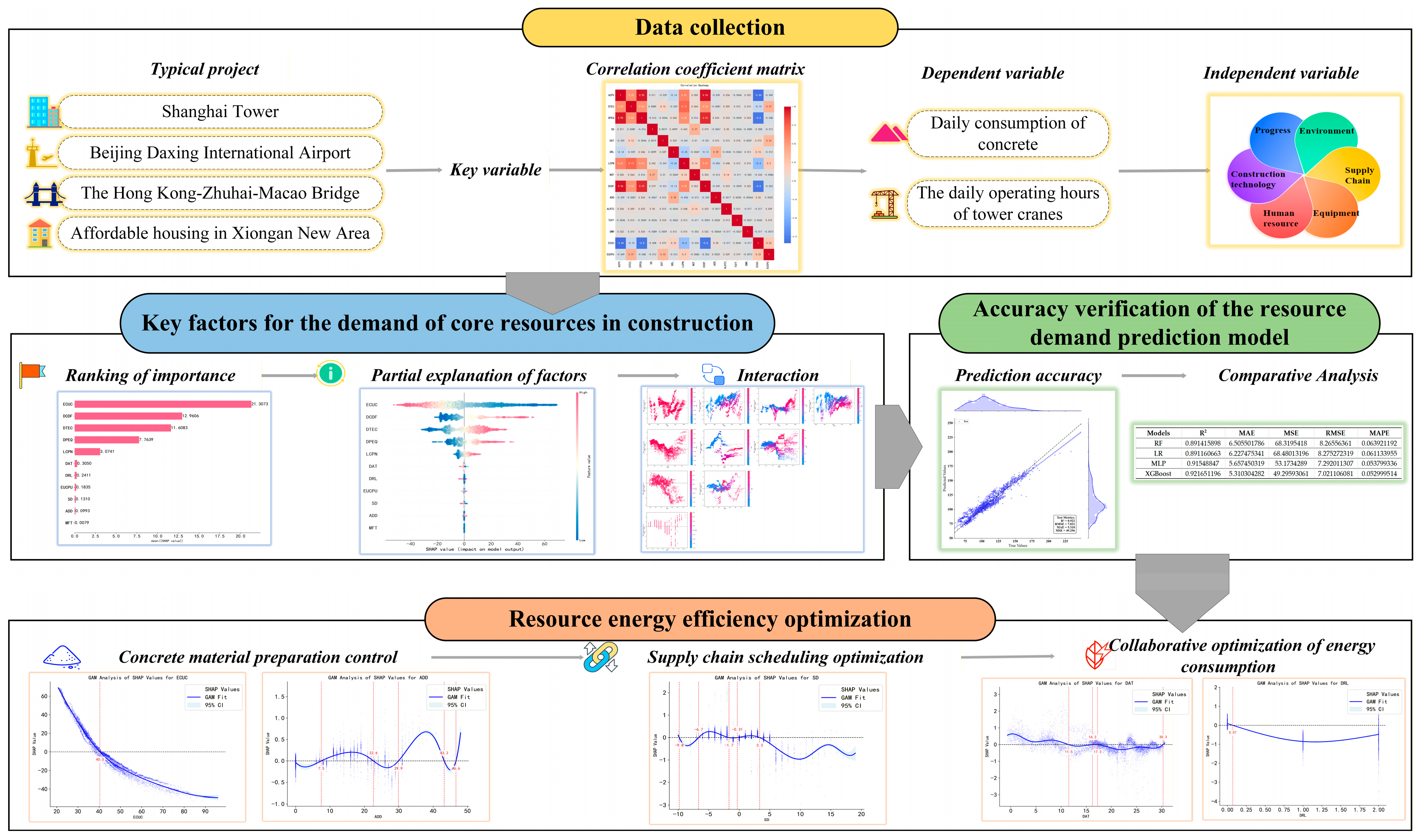
Figure 1. Research process.
Buildings 16 00316 g001
Figure 2. Scatter plot of predicted vs. actual concrete consumption.
Buildings 16 00316 g002
Figure 3. Feature importance ranking.
Buildings 16 00316 g003
Figure 4. SHAP beeswarm plot for concrete resources.
Buildings 16 00316 g004
Figure 5. SHAP interaction value matrix for feature pairs.
Buildings 16 00316 g005
Figure 6. Network diagram of interaction effects among the top five features.
Buildings 16 00316 g006
Figure 7. GAM analysis: core process factors.
Buildings 16 00316 g007
Figure 8. GAM dependence plot for DPEQ.
Buildings 16 00316 g008
Figure 9. GAM dependence plot for SD.
Buildings 16 00316 g009
Figure 10. GAM-based analysis of key External Environment Adaptation Layer.
Buildings 16 00316 g010
Table 1. Summary of research data sources.
CategorySpecific Source
Macro-level building material consumption dataNational Bureau of Statistics of China—Consumption of Building Materials and Cement (https://www.stats.gov.cn/) (Accessed on 21 October 2025)
Background data for iconic skyscraper projectsShanghai Tower Construction & Development Co., Ltd./Shanghai Construction Group official releases (https://scdri.scg.com.cn/)
Large-scale public infrastructure project dataBeijing Daxing International Airport Authority official website (https://www.bdia.com.cn/)
Cross-sea mega-project background dataHong Kong–Zhuhai–Macao Bridge Authority official portal (https://www.hzmb.hk/)
New district affordable housing/prefabricated engineering dataXiong’an New Area Management Committee website—Construction Updates (http://www.xiongan.gov.cn/)
Policies and construction management specificationsMinistry of Housing and Urban–Rural Development—Department of Engineering Quality and Safety Supervision (https://www.mohurd.gov.cn/)
Energy consumption and energy-saving standardsChina Association of Building Energy Efficiency/Construction Industry Energy Conservation Standards (http://www.cabee.org/)
Scientific research/daily high-frequency monitoring dataCarbon Monitor–Real-Time CO2 Emissions Data Platform (https://carbonmonitor.org/)
Table 2. Project collection time and valid data.
Project NameCommencement DatePeriod of Data CollectionValid Data Volume
Shanghai Tower2008.11.292011.4.1–2019.12.312600
Beijing Daxing International Airport2014.12.262016.1.1–2019.9.301369
Hong Kong–Zhuhai–Macao Bridge2009.12.152009.12.15–2018.10.242800
Affordable Housing in the Xiong’an New Area2020.3.202020.5.1–2024.10.31645
Table 3. Variable definitions and quantification criteria for the prediction model.
CategoryVariable NameUnitDescriptionSource/MeasurementIndependence from Target
Construction TechnologyElectricity Consumption per Unit Concrete (ECUC)kWh/m3The electricity consumed for concrete operations per cubic meter of planned concreteTotal construction electricity consumption ÷ Actual amount of concrete pouredIndependent.
Denominator uses planned quantity (DPEQ), not actual consumption
Daily Total Electricity Consumption (DTEC)kWhTotal site-wide electricity consumptionTotal electricity quantity of each sub-itemIndependent.
Direct measurement, independent of concrete volume
Supply ChainDaily Concrete Delivery Frequency (DCDF)CountNumber of ready-mix concrete truck deliveries scheduled for the dayNumber of batches arrivingIndependent.
A planned supply-chain variable
Average Delivery Delay (ADD)minutesAverage delay per delivery truck against the scheduled arrival time( max 0 , actual planned ) /number of batchesIndependent.
Measures logistics performance, not consumption
EnvironmentDaily Average Temperature (DAT)°CAverage ambient temperatureOn-site weather station recordsIndependent.
External environmental factor
Daily Rainfall Level (DRL)mmTotal precipitationOn-site weather station recordsIndependent. External environmental factor
LaborLabor Count on Concrete Pouring (LCPN)CountNumber of workers assigned to concrete pouring tasksTake it straight from the ledgerIndependent.
A planned resource allocation variable
ScheduleSchedule Deviation (SD)%Progress status relative to the baseline scheduleActual progress schedule—Planned progress scheduleIndependent.
Measures progress, not resource use
Daily Planned Engineering Quantity (DPEQ)m3Volume of concrete planned to be poured for the day, as per the construction scheduleConstruction plan givenIndependent.
The primary planned input, not a measured outcome
EquipmentEquipment Usage Cost Per Unit (EUCPU)CNY
/hour
Operational cost rate of key equipmentEquipment cost/Project outputIndependent.
A fixed cost parameter
Mixing Equipment Failure Times (MFT)CountNumber of failures or stoppages of mixing equipmentCount the number of outage eventsIndependent.
Measures equipment status, not output
Table 4. Hyperparameter tuning space for the XGBoost model.
HyperparameterDescriptionTuning Range
learning_rate (η)Learning rate: Controls the weight of each decision tree[0.01, 0.3]
max_depthMaximum depth of a single decision tree[3, 10]
min_child_weightMinimum sum of sample weights required for a leaf node[1, 10]
subsampleProportion of sample subsets used for training each tree[0.7, 1.0]
colsample_bytreeProportion of feature subsets used for training each tree[0.7, 1.0]
reg_alpha (L1)Weight of L1 regularization term: Enhances model sparsity[0, 1]
reg_lambda (L2)Weight of L2 regularization term: Prevents overfitting[1, 5]
Table 5. Model performance comparison.
ModelsR2MAEMSERMSEMAPE
RF0.8914158986.50550178668.31954188.265563610.063921192
LR0.8911606636.22747534168.480131968.2752723190.061133955
MLP0.915488475.65745031953.17342897.2920113070.053799336
XGBoost0.9216511965.31030428249.295930617.0211060810.052999514
Disclaimer/Publisher’s Note: The statements, opinions and data contained in all publications are solely those of the individual author(s) and contributor(s) and not of MDPI and/or the editor(s). MDPI and/or the editor(s) disclaim responsibility for any injury to people or property resulting from any ideas, methods, instructions or products referred to in the content.