Nonlinear and Congestion-Dependent Effects of Transport and Built-Environment Factors on Urban CO₂ Emissions: A GeoAI-Based Analysis of 50 Chinese Cities

Abstract

Understanding how transport conditions and the built environment shape urban CO₂ emissions is critical for low-carbon urban development. This study analyses CO₂ emission intensity across fifty major Chinese cities using integrated ODIAC emissions, VIIRS night-time lights, traffic performance indicators, built-environment morphology, population/POI structure, and socioeconomic controls. We develop a GeoAI workflow that couples XGBoost modelling with SHAP interpretation, congestion-based city grouping, and 1 km grid-level GNNWR to map intra-urban spatial non-stationarity. The global model identifies night-time light intensity as the strongest predictor, followed by population density and building density. SHAP results reveal pronounced nonlinearities, with high sensitivity at low–medium levels and diminishing marginal effects as activity and density increase. Although transport indicators are less influential in the aggregate model, their roles differ across congestion regimes: in low-congestion cities, emissions align more consistently with overall activity intensity, whereas in high-congestion cities they respond more strongly to population distribution, motorisation, and built-form intensity, with less stable relationships. Grid-level GNNWR further shows that key mechanisms are spatially uneven within cities, with local effects concentrating in specific cores and corridors or fragmenting across multiple subareas. These findings demonstrate that emission drivers are context-dependent across and within cities. Accordingly, uncongested cities may gain more from activity-related energy-efficiency measures, while highly congested cities may require congestion-sensitive land-use planning, spatial-structure optimisation, and motorisation control. Integrating explainable GeoAI with regime differentiation and spatial heterogeneity mapping provides actionable evidence for targeted low-carbon planning.

1. Introduction

Against the backdrop of China’s national strategies for carbon peaking and carbon neutrality, a critical challenge for contemporary urban development is how to effectively curb the growth of urban carbon emissions while sustaining economic expansion. Cities are major contributors to climate change, as urban activities account for approximately 70% of global fossil fuel CO₂ emissions, with transport and buildings together representing the fastest-growing sources of urban emissions (https://www.unep.org/explore-topics/resource-efficiency/what-we-do/cities-and-climate-change (accessed on 16 November 2025)). In China, urban transport has become an increasingly important source of carbon emissions under conditions of rapid motorisation, rising travel demand, and persistent peak-hour congestion, as evidenced by recent spatiotemporal studies linking traffic emissions with built-environment characteristics and congestion patterns [1,2,3]. As the primary spatial carriers of energy consumption and human activities, cities generate the majority of national economic output and, at the same time, account for more than 70% of total energy use and greenhouse gas emissions [4,5,6]. Their mitigation performance therefore plays a decisive role in achieving national carbon targets. Compared with traditional industrial and power sectors, the urban system shaped jointly by travel behaviour and spatial development, often referred to as the transportation and built-environment nexus, has increasingly become an important contributor to the continued rise in urban carbon emissions [7,8,9].

The rising level of motorisation and increasing travel demand, together with persistently saturated peak-hour conditions, have significantly expanded the contribution of the transport sector to urban carbon emission growth [10,11]. At the same time, built-environment characteristics such as high development intensity, functionally segregated land-use patterns, and pronounced jobs–housing imbalance tend to lengthen commuting distances and reinforce dependence on private automobiles, thereby raising transport energy consumption and associated carbon emissions on the demand side [12,13]. Hence, the focus of research needs to shift from merely describing the absolute level of urban carbon emissions to quantitatively identifying the mechanisms through which transport features and built-environment factors affect emissions, while controlling for socioeconomic differences, and to assessing their relative contributions to inter-city variation in carbon emission intensity. Such insights are crucial for designing typology-based low-carbon transport policies and for guiding urban spatial planning.

In parallel, the rapid growth of remote sensing observations, traffic big data, and various forms of urban spatial information has provided new methodological opportunities for analysing the complex processes underlying urban carbon emissions [14,15]. Geographical artificial intelligence (GeoAI) integrates geographic thinking with machine learning techniques and enables, on the one hand, the integration of heterogeneous multi-source datasets, such as carbon emission grids, night-time light imagery, population and POI data, building morphology indicators, and traffic performance metrics, within a unified spatial framework [16,17,18]. On the other hand, it allows the use of nonlinear models to capture the coupled relationships among high-dimensional variables [19]. At the same time, Chinese cities exhibit substantial diversity in both traffic conditions and patterns of spatial development. Some mega-cities have long operated under severe congestion and high-density development [20,21], whereas others experience only moderate congestion or relatively smooth traffic conditions, with pronounced differences in levels of motorisation and the provision of public transport [22,23]. This implies that the direction and magnitude of the effects of similar transport and spatial indicators may vary across cities, and that the drivers of urban carbon emissions are strongly context-dependent and spatially heterogeneous. Relying solely on a single global model tends to compress such differences into an average effect, making it difficult to answer policy-relevant questions such as which cities are predominantly driven by transport-system factors and which are more strongly shaped by spatial-structural factors. It is therefore necessary to complement GeoAI-based global nonlinear modelling with city typologies derived from traffic performance and with spatial heterogeneity analysis in order to identify the differentiated impacts of transport characteristics and built-environment features on carbon emissions under different congestion contexts.

According to that, this study selects the top 50 Chinese cities by GDP as the study area and constructs a multi-source urban database integrating ODIAC CO₂ emission grids, VIIRS night-time light imagery, road-traffic performance indicators, gridded population and POI data, building density and height metrics, and socioeconomic statistics. On this basis, we develop a GeoAI-based analytical framework that links global modelling, mechanism interpretation, congestion-regime differentiation, and spatial heterogeneity analysis. Specifically, we first employ an XGBoost model to identify the main determinants of urban CO₂ emission intensity and use SHAP values to interpret nonlinear effects and potential thresholds of transport and built-environment factors. We then classify cities into congestion regimes using the peak-hour travel delay index and estimate group-specific models to examine how driver importance and response patterns shift across traffic contexts. Finally, to move beyond administrative averages and reveal “where and how” mechanisms operate within cities, we conduct a 1 km grid-level analysis using GNNWR to map spatially varying relationships and characterise intra-urban non-stationarity, providing spatially actionable evidence for differentiated low-carbon planning and transport–land-use policy.

2. Literature Review

2.1. Transportation System with Urban Carbon Emissions

The transportation system is a major source of urban carbon emissions, and its underlying mechanisms have been widely examined in existing studies [24,25]. Prior study generally shows that factors such as vehicle ownership, travel distance, travel mode structure, road operating speed, and peak-hour congestion levels directly influence energy consumption and carbon emissions in the transport sector [26,27,28]. Traffic congestion increases emission intensity by reducing average speeds and increasing idling time and acceleration events, whereas the supply of public transport and the configuration of road infrastructure have been shown to mitigate the growth of transport-related emissions to some extent [29]. Despite these insights, most studies rely on linear or quasi-linear models or focus on a limited number of case cities, which constrains their ability to capture the nonlinear effects of transport characteristics and to compare how these mechanisms vary across different traffic operation contexts.

Recent studies increasingly indicate that the relationship between transport conditions and carbon emissions is nonlinear and may exhibit threshold behaviour. Empirical evidence suggests that congestion and traffic operating conditions exert relatively modest emission impacts under low-delay or free-flow regimes, whereas emission intensity increases disproportionately once congestion exceeds certain critical levels due to sharp speed reductions, frequent acceleration–deceleration cycles, and increased idling. Such regime-dependent emission responses have been reported in city-level and network-based analyses of transport emissions [20,21,24,25]. However, most existing studies focus on individual cities or transport subsystems, which limits the ability to generalise these threshold effects across cities with different congestion contexts.

2.2. Urban Built Environment, Spatial Structure, and Carbon Emissions

The built environment, as a key component of urban spatial structure, shapes urban carbon emissions indirectly by influencing travel demand, travel mode choice, and building energy use [30]. Existing studies have shown that population density and building density may exhibit nonlinear, and in some cases even opposite, effects under different urban contexts: moderate densities tend to shorten average travel distances, whereas extremely high densities can lead to excessive activity concentration and more severe traffic congestion, thereby increasing emission intensity. Land-use mix and jobs–housing balance are generally considered to reduce rigid commuting demand and increase the share of public and non-motorised transport, thus helping to curb transport-related carbon emissions [31]. However, most of these studies focus on the directional effect of individual built-environment attributes, and there is still a lack of systematic synthesis regarding the interactions among different attributes, potential threshold effects, and generalisable patterns across cities.

As research has increasingly recognised the complexity of urban systems, the coupled influences of transport systems and the built environment have attracted growing attention. Existing studies indicate that urban spatial structure not only shapes travel demand but also affects the formation of traffic congestion, while the performance of the transport system largely reflects the combined outcomes of spatial layout and development intensity. Urban carbon emissions are therefore often the result of the joint effects of these two dimensions. However, studies that incorporate both factors within a unified analytical framework remain limited, and the nonlinear relationships and complex interactions between them have not been sufficiently examined. Moreover, empirical evidence on whether different types of cities (for example, those with varying levels of congestion or motorisation) exhibit systematically different carbon-emission mechanisms is still scarce. As a consequence, current findings tend to reflect an “average city,” providing only limited support for typology-based and context-sensitive policy formulation.

An emerging body of literature further suggests that the effects of built-environment characteristics on carbon emissions are often nonlinear and subject to threshold or saturation effects. Moderate levels of population density, development intensity, and functional mix are frequently associated with reduced travel distances and improved transport efficiency, whereas excessive concentration may intensify congestion pressure and energy demand, leading to higher emission intensity. Empirical studies have reported such non-monotonic or diminishing-return patterns for density-related and spatial-structure indicators in Chinese cities and urban agglomerations [9,12,26]. Nevertheless, existing evidence remains fragmented and largely attribute-specific, with limited attention paid to how such threshold behaviours vary systematically across cities with different congestion regimes

2.3. Applications of GeoAI in Urban Carbon-Emission Studies

With the rapid growth of night-time light imagery, remote sensing grids, traffic big data, and multi-source points-of-interest (POI) information, GeoAI has become an increasingly influential paradigm for urban carbon-emission research by enabling multi-source geospatial data fusion, nonlinear learning, and spatially explicit mechanism discovery [16,32,33]. Tree-based machine learning models such as XGBoost and Random Forest can accommodate high-dimensional and collinear predictors and capture nonlinear responses and threshold behaviours that are difficult to represent with conventional linear specifications [21]. Alongside these advances, the field is shifting from purely “prediction-oriented” applications toward interpretation- and decision-oriented analyses that aim to explain how transport conditions and built-environment structures shape emissions under different urban contexts. Explainable-AI techniques such as SHAP further support this shift by providing feature-level attributions and revealing nonlinear sensitivities and interaction patterns, thereby improving the transparency of complex models for planning-relevant interpretation.

Despite these advances, important gaps remain. Many GeoAI studies still treat carbon-emission modelling mainly as a prediction task, reporting high accuracy or a single global importance ranking. Such summaries are useful, but they often mask the fact that emission drivers may operate differently across cities with different congestion or motorisation conditions. In addition, spatial information is frequently incorporated only through city-level aggregates, so the analysis cannot show where within a city certain built-environment or activity factors matter most, nor whether their effects are stable or highly variable across neighbourhoods. As a result, relatively few studies bring together three elements in one workflow: an interpretable nonlinear model, a context-based city typology (e.g., congestion regimes), and grid-level mapping of spatially varying relationships. Without this integration, GeoAI evidence is harder to translate into targeted planning actions and transport–land-use policies.

3. Method

3.1. Study Area

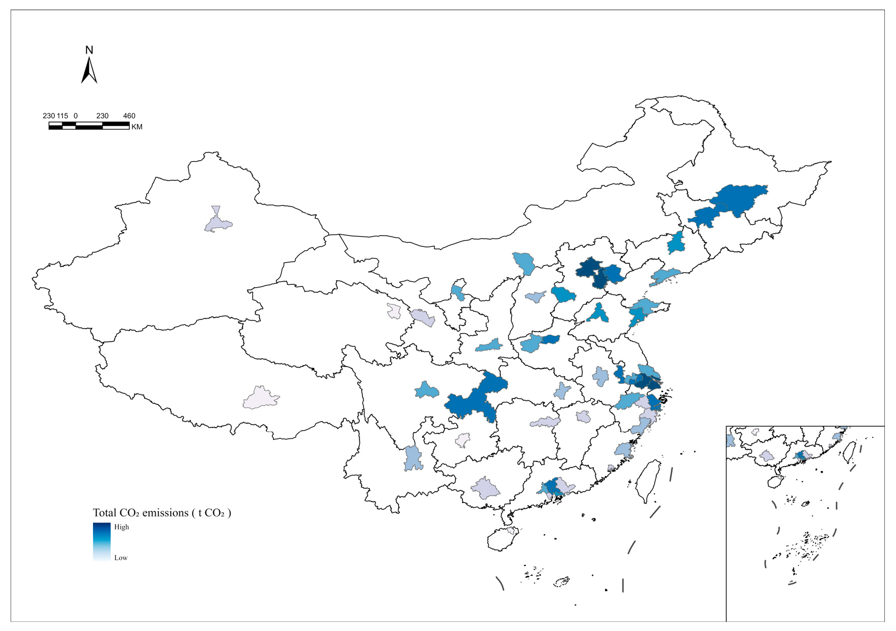
This study adopts the 50-city system reported in the Traffic Analysis Report of Major Chinese Cities released by Amap (Gaode) (https://report.amap.com/diagnosis/index.do (accessed on 1 December 2025)) as the study area. In the report, cities are ranked using a composite index that combines development characteristics (e.g., GDP, urban influence, and built-up population) with traffic-related attributes (e.g., vehicle ownership, the size of core travel zones, and traffic density). Based on this ranking, we select the top 50 cities, covering municipalities directly under the central government, vice-provincial cities, and economically strong prefecture-level cities. The sample includes national and regional centres such as Beijing, Shanghai, Shenzhen, Guangzhou, Hohhot, Xining, Urumqi, and Lhasa (Figure 1). Collectively, these cities represent China’s most economically dynamic urban group, where population and industries are highly concentrated and a substantial share of national energy consumption and carbon emissions is generated.

Moreover, the selected cities exhibit pronounced diversity in natural conditions, economic development, industrial structure, city size, transport systems, and built-environment form. The sample includes megacities with compact urban structure and relatively well-developed rail transit systems, export-oriented manufacturing cities with strong road-based commuting and freight activity, and western/northeastern cities shaped by terrain constraints, climate, and industrial legacy. This heterogeneity provides a solid empirical basis for examining nonlinear and context-dependent relationships between transport conditions, the built environment, and urban CO₂ emissions and improves the robustness and potential transferability of the modelling results.

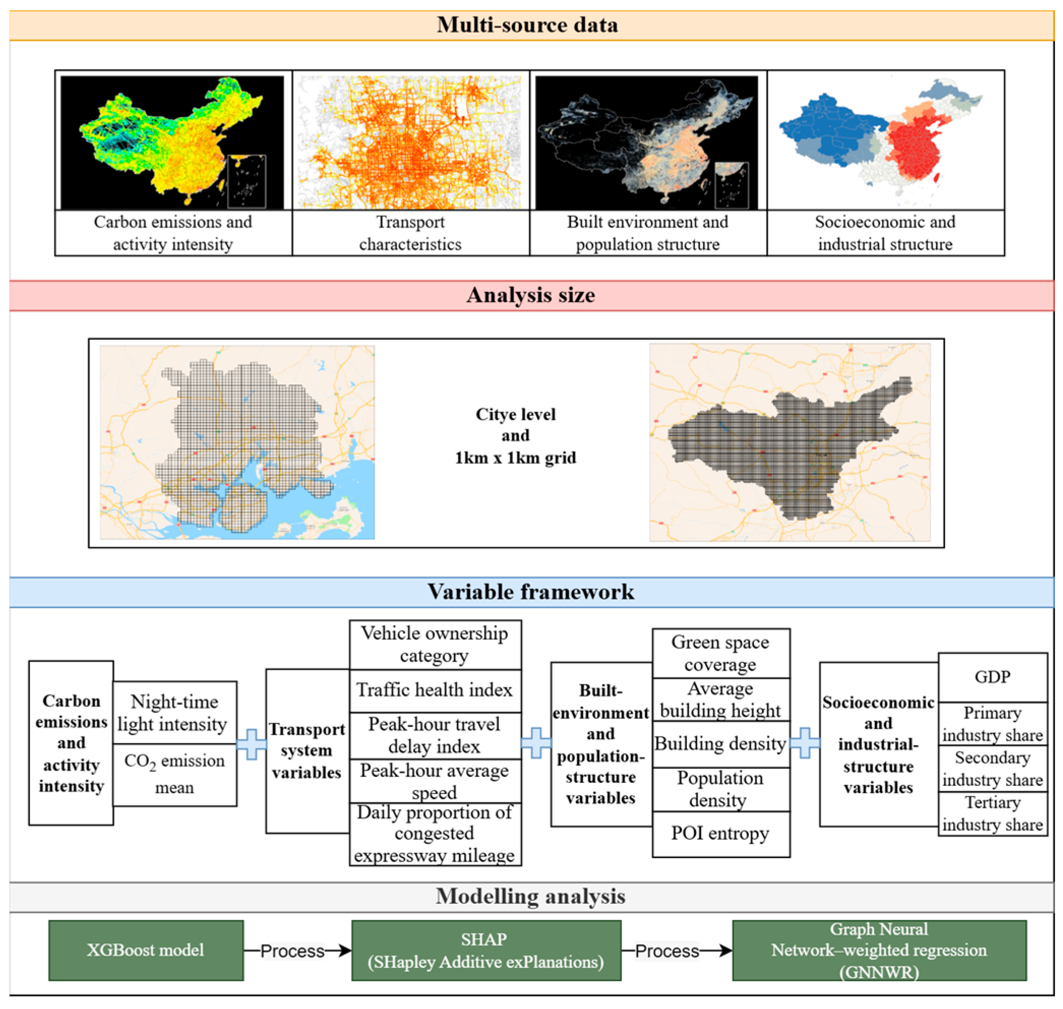
As summarised in the conceptual framework (Figure 2), this study integrates multi-source datasets describing carbon emissions and activity intensity, transport performance, built-environment and population structure, and socioeconomic/industrial conditions and analyses them at two complementary spatial scales: the city administrative level and the 1 km × 1 km grid level. The framework further links these data to a GeoAI workflow consisting of (i) city-level nonlinear modelling to identify key determinants, (ii) explainable interpretation to diagnose nonlinear responses and thresholds, (iii) congestion-regime differentiation to compare mechanisms across traffic contexts, and (iv) grid-level spatial heterogeneity modelling to reveal intra-urban non-stationarity. This design ensures that the analysis is not limited to “average-city” relationships and provides spatially explicit evidence to support differentiated low-carbon planning and transport–land-use policy.

3.2. Multi-Source Data Collection

This study selects the top 50 Chinese cities as the research sample and builds a comprehensive multi-source urban database by integrating ODIAC CO₂ emission grids, VIIRS night-time light imagery, built-environment indicators, population grids, POI datasets, traffic performance metrics, and statistical yearbook information within consistent prefecture-level administrative boundaries. All datasets are harmonised to the same reference year (2024) and aggregated to the city-administrative level, resulting in a cross-sectional dataset of 50 cities.

Following the analytical logic of “carbon emissions–transport characteristics–built environment–socioeconomic conditions”, all variables are organised into three groups: the dependent variable, core explanatory variables (transport and built-environment attributes), and control variables. Redundant or strongly collinear indicators are examined and filtered in order to obtain a concise, well-structured dataset with consistent measurement scales that is suitable for GeoAI-based modelling.

3.2.1. Carbon Emissions and Activity Intensity

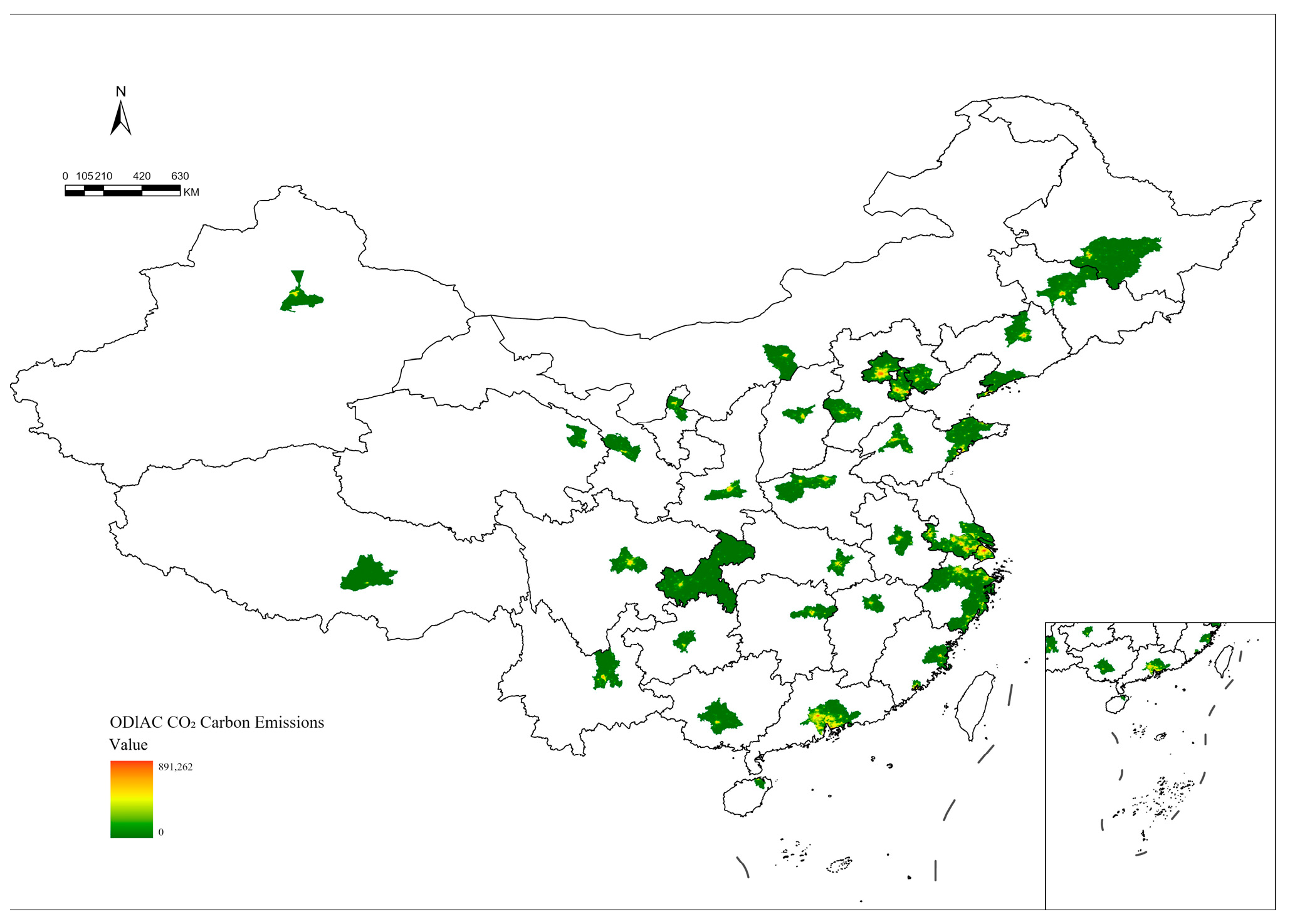
Urban carbon-emission data are obtained from the annual ODIAC CO₂ emission grid, which provides fossil fuel CO₂ emissions in 1 km × 1 km resolution [34,35]. For each of the fifty cities, the raster for the study year is overlaid with the administrative boundary, and pixel values within the boundary are aggregated using an area-weighted summation to derive total CO₂ emissions (kg CO₂) (Figure 3). To enable comparison across cities of different sizes, total emissions are normalised by the built-up area, which is delineated using a raster-based urban mask derived from impervious surface coverage and night-time light intensity, to produce area-normalised CO₂ emission intensity (kg CO₂/km²), which serves as the primary indicator of emission intensity. Total emissions are retained only for descriptive comparison. To improve the statistical distribution and reduce the influence of extreme values, the mean CO₂ emission variable is transformed using the natural logarithm before modelling, and this log-transformed value is used as the dependent variable in the XGBoost model.

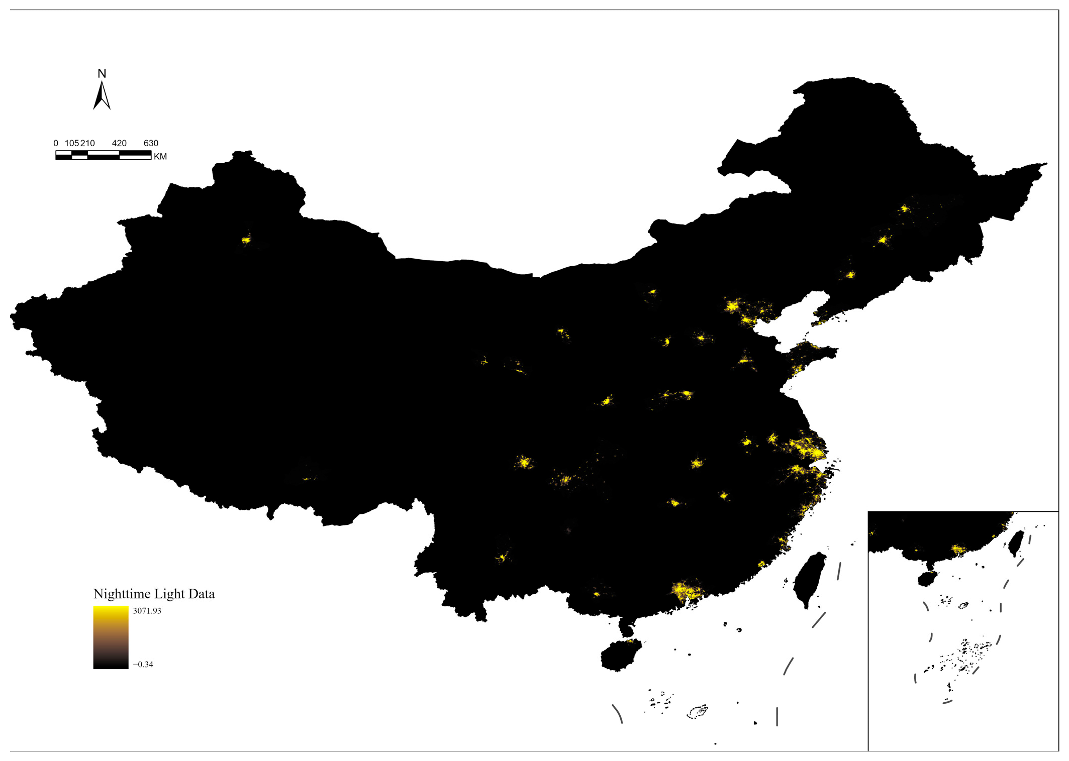
Night-time light data are sourced from VIIRS night-time light imagery (https://eogdata.mines.edu/products/dmsp/ (accessed on 2 December 2025)) [36,37] (Figure 4). The raster is clipped to each city boundary, and valid pixels are summarised to obtain mean radiance intensity, which is used as a proxy for human activity and energy-use intensity. Both the VIIRS and ODIAC rasters are aligned to the administrative boundaries after coordinate checking and, where necessary, reprojection, with all raster layers resampled to a common 1 km grid prior to aggregation to ensure spatial consistency between raster and vector datasets. The resulting indicators of CO₂ emission intensity and night-time light activity are compiled into a uniform city-level dataset for subsequent modelling (

Table 1. Variables for carbon emissions and activity intensity.

Category	Indicator	Description	Type/Unit
Carbon emissions	Area-normalised CO2 emission intensity	Area-normalised CO2 emissions (kg CO2 per km2) derived from ODIAC grids; used as the dependent variable	Continuous (kg CO2/km2), log-transformed in modelling
Economic activity proxy	Night-time light intensity (mean)	Average VIIRS night-time light value within the built-up area; proxy for human activity and energy use intensity	Continuous

).

3.2.2. Transport Characteristics

Transport-related indicators are used to characterise the level of motorisation and the operating conditions of the urban road network and form one of the core groups of explanatory variables in this study. Data on vehicle ownership category, traffic health index, year-on-year change in the traffic health index, peak-hour travel delay index, year-on-year change in the delay index, peak-hour average speed, public transport travel satisfaction index, and daily proportion of congested expressway mileage are obtained from the Traffic Analysis Report of Major Chinese Cities 2024 published by Amap (Gaode) (https://report.amap.com/diagnosis/index.do (accessed on 5 December 2025)).

Vehicle ownership is classified into ordered categories and encoded as an ordinal variable to reflect differences in motorisation levels across cities. The traffic health index and its year-on-year change summarise overall traffic efficiency, operational order, and travel experience, representing the general performance of the urban road network and its recent evolution.

To capture different aspects of congestion, several additional indicators are used. The peak-hour travel delay index and its annual change measure the severity and temporal change in morning and evening peak congestion, with higher values indicating greater time loss and lower network efficiency. Peak-hour average speed complements this by describing congestion from a speed perspective. The daily proportion of congested expressway mileage reflects the share of expressway segments operating under congested conditions and captures congestion pressure associated with intercity commuting and long-distance travel. This indicator is expressed as a fraction between 0 and 1 rather than a percentage, and the same scale is used consistently throughout the analysis.

In the final model specification, the vehicle ownership category, traffic health index, peak-hour travel delay index, peak-hour average speed, and daily proportion of congested expressway mileage are retained as core transport variables, while other indicators are used for diagnostic and robustness checks. Together, these variables describe the transport system from the perspectives of motorisation level, urban road congestion, and expressway congestion and provide an empirical basis for analysing how traffic conditions are related to differences in CO₂ emission intensity across cities. The transport variables used in the model are summarised in

Table 2. Transport system variables.

Category	Indicator	Description	Type/Unit
Motorisation level	Vehicle ownership category	City-level motorisation classified into ordered bins (<2 M, 2–3 M, 3–4 M, >4 M vehicles)	Ordinal categorical variable
Overall road-network performance	Traffic health index	Composite measure of traffic efficiency, operational order, and travel experience	Continuous
Urban road congestion	Peak-hour travel delay index	Congestion severity during morning/evening peaks	Continuous
	Peak-hour average speed	Average operating speed during peak periods	km/h
Expressway congestion	Daily proportion of congested expressway mileage	Share of expressway segments operating under congested conditions	-

.

3.2.3. Built Environment and Population Structure

Indicators of the built environment and population spatial structure are used to describe the physical form of cities, the intensity of land development, and the distribution of population activities. These variables serve as important intermediaries through which transport conditions influence carbon-emission outcomes. The indicator system constructed in this study includes measures of green coverage, building morphology, population density, and functional mix.

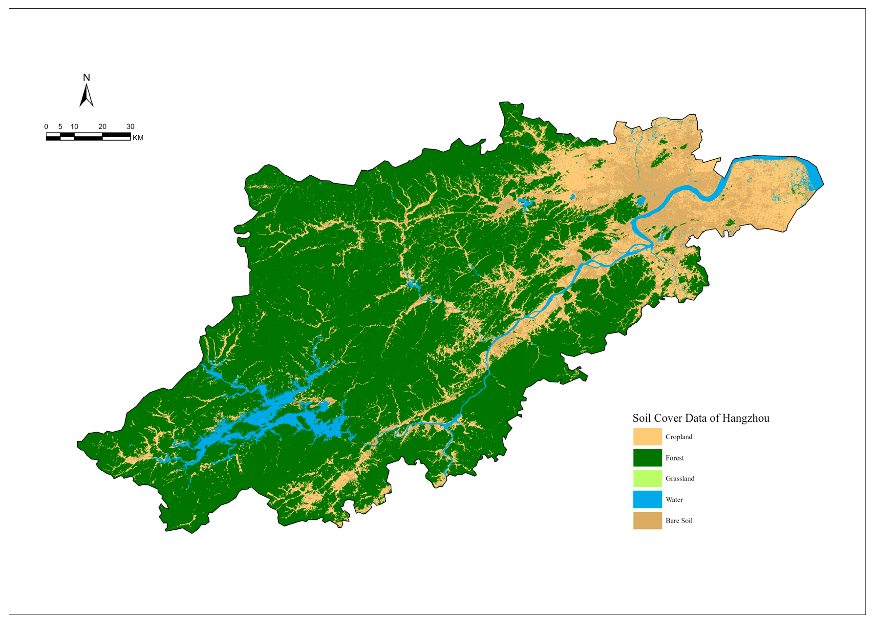
Green space coverage is derived from a 30 m resolution national land-cover dataset [38]. The land-cover raster is overlaid with each city’s administrative boundary, and pixels classified as forests, shrubs, grasslands or wetlands are identified as green space. The proportion of green space pixels among all valid pixels within the boundary is computed as the city’s green space coverage (Figure 5).

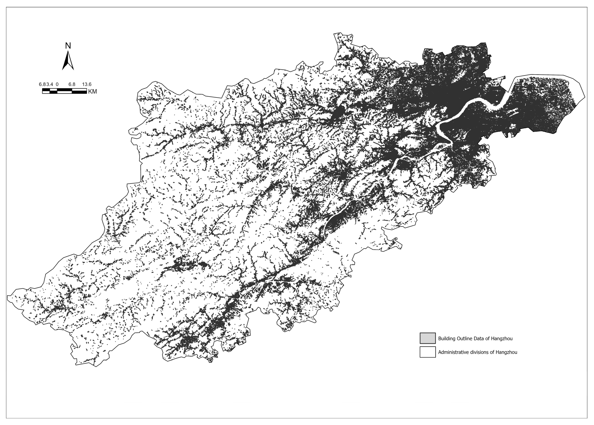
Building morphology indicators are obtained from the 3D-GloBFP building dataset (building height of Asia in 3D-GloBFP) [39] (Figure 6). Building footprints within each administrative boundary are extracted, and their total footprint area is divided by the built-up area to calculate building density. The mean building height is computed from the height attribute of all valid building polygons, representing the vertical dimension of development intensity.

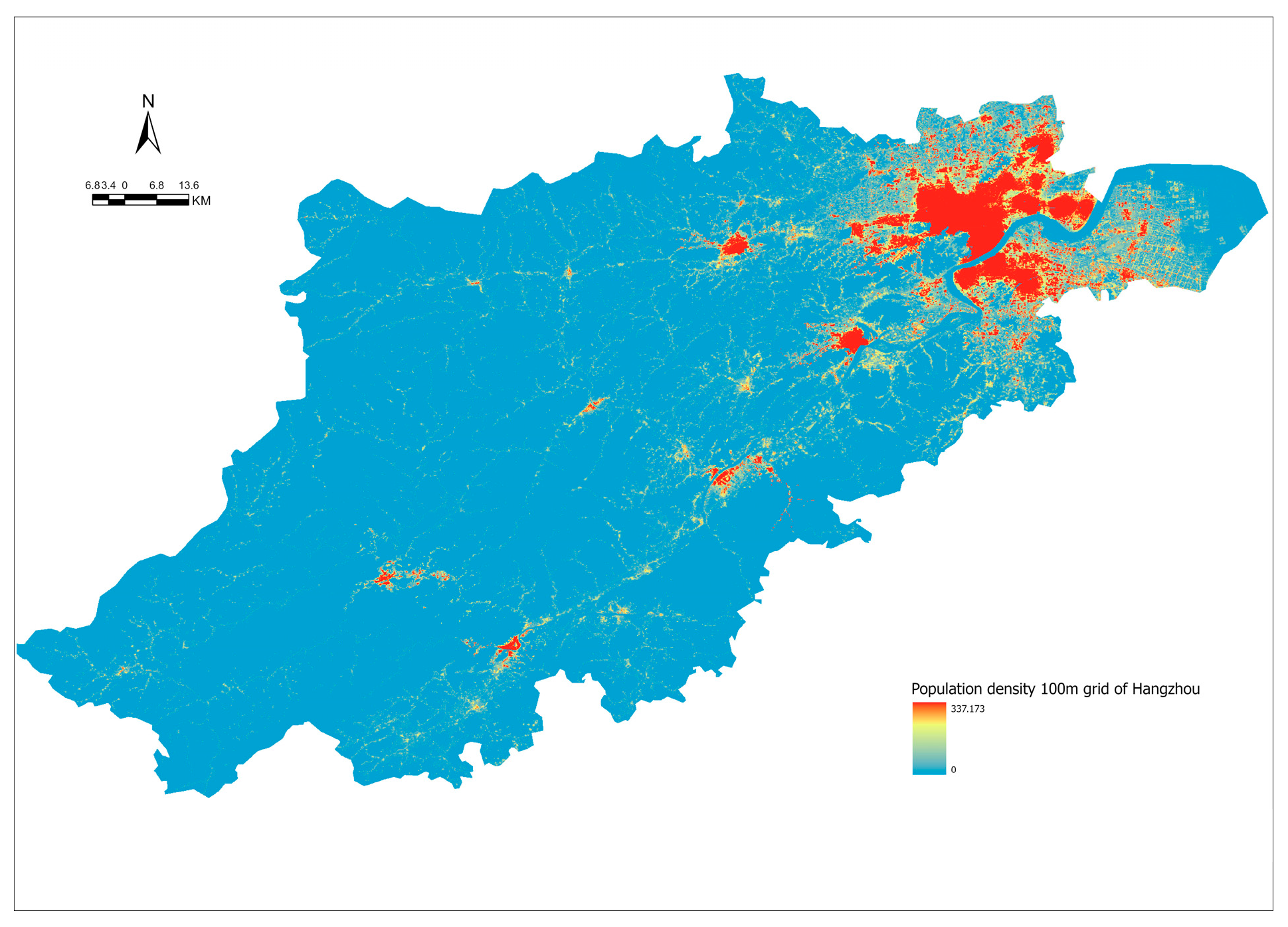
Population density is calculated using a 100 m resolution gridded population dataset [40]. Population pixels are clipped to the built-up area of each city and aggregated to obtain total population, which is then divided by the built-up area to derive population density (persons/km²) (Figure 7). This grid-based measure better reflects the actual distribution of population within active urban space than traditional administrative-density measures.

Functional structure is captured using POI entropy. POI data are collected through the Amap API (https://lbs.amap.com/demo/javascript-api/example/poi-search/polygon-search (accessed on 4 December 2025)), classified into major functional categories and aggregated at the city level. Entropy is computed based on the proportion of each POI category, with higher values indicating a more diversified and spatially balanced urban functional structure.

Because area-based and total-quantity indicators such as total population, total POI count, and total building footprint are highly correlated with density measures, the modelling analysis focuses on structural variables including green space coverage, building density, average building height, population density, and POI entropy. Quantity-based variables are used only for diagnostic and descriptive purposes. The variables used in this group are summarised in

Table 3. Built-environment and population-structure variables.

Category	Indicator	Description	Type/Unit
Built environment	Green space coverage	Proportion of green area within the city’s administrative boundary	%
	Average building height	Mean height of buildings within the built-up area	m
	Building density	Ratio of total building footprint area to built-up area	–
Population spatial structure	Population density (grid-based)	Population per km2 within the built-up area, derived from TIFF population grids	persons/km2
Functional structure	POI entropy	Entropy index based on the distribution of POI categories; higher values indicate a higher degree of land-use and functional mix	–

.

3.2.4. Socioeconomic and Industrial Structure

Socioeconomic and industrial structure indicators are included to control for the systematic influence of economic scale and industrial composition on urban carbon emissions. City-level GDP reflects the overall size of the urban economy and, together with population density, characterises the economic and demographic context of each city. The shares of the primary, secondary, and tertiary industries capture differences in economic structure, distinguishing energy-intensive industrial cities from more service-oriented, lower-carbon cities. Data on GDP, permanent population, administrative area, population density, and industrial structure are obtained from the 2024 local statistical yearbooks of each city. The variables in this group are summarised in

Table 4. Socioeconomic and industrial-structure variables.

Category	Indicator	Description	Type/Unit
Economic scale	GDP	Gross domestic product of the city	billion RMB
Industrial structure	Primary industry share	Proportion of GDP generated by the primary sector	%
Industrial structure	Secondary industry share	Proportion of GDP generated by the secondary sector	%
Industrial structure	Tertiary industry share	Proportion of GDP generated by the tertiary sector	%

.

3.2.5. Variable Classification and Preprocessing

Drawing on the multi-source data described above, the indicator system is organised according to a hierarchical logic of “dependent variable–transport characteristics–built environment–socioeconomic conditions”. The dependent variable is defined as the natural logarithm of area-normalised CO₂ emissions (kg CO₂ per km² of built-up area), used to represent urban carbon emission intensity, in a manner consistent with the study’s focus on how transport conditions and built-environment structure shape the spatial concentration of emissions within cities. Unlike GDP-normalised or per capita emission indicators commonly used to assess economic or individual carbon efficiency, the selected measure is intended to capture how transport conditions and built-environment characteristics shape the spatial intensity of emissions within urban areas. Transport-related indicators constitute the first group of core explanatory variables and are used to capture the direct impacts of traffic conditions and congestion on emissions. Built-environment and population spatial-structure indicators form the second group of core explanatory variables and describe differences in urban density, form, and functional mix. Socioeconomic and industrial structure indicators serve as control variables to account for systematic effects of economic scale and industrial composition.

Before modelling, all continuous variables are subjected to missing-data treatment and outlier checking; the dependent variable is log-transformed to reduce right-skewness and the influence of extreme values, and then all variables are standardised to remove scale differences. Ordered categorical variables, such as vehicle ownership categories, are encoded as ordinal variables. To avoid redundancy and scale dominance in the subsequent modelling, total-quantity variables and strictly constrained components, such as total CO₂ emissions, total population, and total POI count, are not included in the set of candidate explanatory variables. The resulting cross-sectional dataset therefore uses CO₂ emission intensity as the dependent variable, transport and built-environment attributes as core explanatory variables, and night-time light and industrial structure as key controls, providing a consistent empirical basis for the subsequent XGBoost modelling, SHAP interpretation, and group-wise analysis.

In addition to individual variables, three composite indices are constructed to support comparative interpretation of spatial heterogeneity results. A density index is defined by combining population density and building density; an activity index integrates night-time light intensity and POI entropy; and a green index is represented by green space coverage. All component variables are standardised using z-score normalisation prior to aggregation, and each composite index is calculated as the unweighted mean of its standardised components.

3.3. Modelling Analysis

To delineate how transport characteristics and the built environment jointly influence urban carbon emissions, this study develops a GeoAI-based modelling framework comprising four sequential components: global factor identification, nonlinear mechanism interpretation, congestion-based city-type differentiation, and grid-level spatial heterogeneity modelling. The framework supports a stepwise investigation that progresses from city-level global estimation to SHAP-based nonlinear interpretation, then to congestion-regime comparisons, and finally to intra-urban nonstationary mechanism mapping using a GeoAI-oriented spatial learning model (GNNWR). Rather than a loose collection of methods, it integrates XGBoost, SHAP, and congestion-based city classification into a coherent workflow, enabling us to capture both the overall drivers of urban CO₂ emission intensity and the context-dependent mechanisms associated with distinct congestion regimes.

3.3.1. XGBoost Model Specification

XGBoost is employed as the primary nonlinear regression model to examine the relationship between urban carbon-emission intensity and the set of transport, built-environment, and socioeconomic variables. For a dataset $\{({\mathrm{x}}_{\mathrm{i}},{\mathrm{y}}_{\mathrm{i}}){\}}_{\mathrm{i}=1}^{\mathrm{N}}$, the XGBoost prediction is expressed as an additive ensemble of regression trees [7,12]:

$${\widehat{\mathrm{y}}}_{\mathrm{i}}=\sum _{\mathrm{t}=1}^{\mathrm{T}}{\mathrm{f}}_{\mathrm{t}}({\mathrm{x}}_{\mathrm{i}}),{\mathrm{f}}_{\mathrm{t}}\in \mathcal{F}$$

(1)

where ${\mathrm{f}}_{\mathrm{t}}$ denotes a regression tree and $\mathcal{F}$ is the functional space of all possible trees.

The model parameters are estimated by minimising the regularised objective:

$$\mathcal{L}=\sum _{\mathrm{i}=1}^{\mathrm{N}}\mathrm{l}({\mathrm{y}}_{\mathrm{i}},{\widehat{\mathrm{y}}}_{\mathrm{i}})+\sum _{\mathrm{t}=1}^{\mathrm{T}}\mathsf{\Omega }({\mathrm{f}}_{\mathrm{t}})$$

(2)

where $\mathrm{l}(\cdot )$ is a differentiable loss function and $\mathsf{\Omega }\left({\mathrm{f}}_{\mathrm{t}}\right)$ penalises model complexity. Hyperparameters (tree depth, learning rate, and number of estimators) are selected through grid search combined with five-fold cross-validation on the training set to prevent overfitting. Model performance is further assessed using a held-out test set, with the dataset randomly split into training (80%) and test (20%) subsets; the random seed is fixed throughout the modelling process given the relatively small cross-sectional sample.

3.3.2. SHAP-Based Model Interpretation

To interpret the nonlinear mechanism captured by XGBoost, SHAP (SHapley Additive exPlanations) is used to decompose the predicted value into feature-level contributions. SHAP represents the model output for city $\mathrm{i}$ as follows [5,41]:

$${\widehat{\mathrm{y}}}_{\mathrm{i}}={\mathsf{\varphi }}_0+\sum _{\mathrm{k}=1}^{\mathrm{K}}{\mathsf{\varphi }}_{\mathrm{k}}^{\left(\mathrm{i}\right)}$$

(3)

where ${\mathsf{\varphi }}_0$ is the baseline prediction and ${\mathsf{\varphi }}_{\mathrm{k}}^{\left(\mathrm{i}\right)}$ is the marginal contribution of feature $\mathrm{k}$.

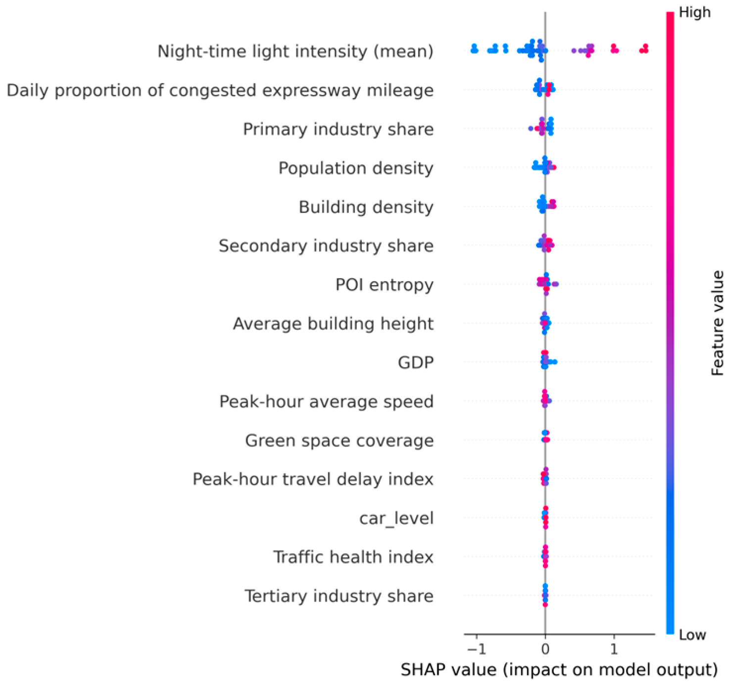
SHAP summary plots are used to assess global importance, while dependence plots reveal nonlinear responses and potential thresholds of congestion, density, and functional-mix indicators.

3.3.3. Congestion-Based City Grouping and Group-Wise Modelling

To assess how traffic conditions modify the determinants of urban CO₂ emission intensity, cities are classified into two congestion groups based on the distribution of the peak-hour travel delay index. Let ${\mathrm{d}}_{\mathrm{i}}$ denote the delay index of city $\mathrm{i}$. The sample median of $\left\{{\mathrm{d}}_{\mathrm{i}}\right\}$ is used as the threshold, dividing the cities into a low-congestion group (${\mathrm{d}}_{\mathrm{i}}\le {\mathrm{P}}_{50}$) and a high-congestion group (${\mathrm{d}}_{\mathrm{i}}>{\mathrm{P}}_{50}$).

For each group, an independent XGBoost model is estimated using the same set of explanatory variables and the same hyperparameter settings as the global model. This allows the relative importance of transport, built-environment, and socioeconomic variables to be compared across different congestion contexts. Differences in model performance, feature importance, and SHAP-based response patterns are then examined to identify how congestion conditions influence the mechanisms linking urban characteristics to CO₂ emission intensity.

3.3.4. GNNWR-Based Grid-Level Spatial Heterogeneity Analysis

While the city-level XGBoost–SHAP analysis identifies global drivers and congestion-regime differences, it cannot capture intra-urban non-stationarity because all variables are aggregated to the administrative level. To reveal how the effects of built-environment and activity-related factors vary across space within cities, this study further conducts a 1 km grid-level spatial heterogeneity analysis using graph neural network–weighted regression (GNNWR).

GNNWR extends geographically weighted modelling by learning spatially varying kernel weights from a graph representation of neighbourhood connectivity [42,43]. For each grid cell $\mathrm{i}$, the local relationship between CO₂ intensity and explanatory variables is modelled as follows [44]:

$${\mathrm{y}}_{\mathrm{i}}={\mathsf{\beta }}_0({\mathrm{u}}_{\mathrm{i}},{\mathrm{v}}_{\mathrm{i}})+\sum _{\mathrm{k}=1}^{\mathrm{K}}{\mathsf{\beta }}_{\mathrm{k}}({\mathrm{u}}_{\mathrm{i}},{\mathrm{v}}_{\mathrm{i}}) {\mathrm{x}}_{\mathrm{i}\mathrm{k}}+{\mathsf{\epsilon }}_{\mathrm{i}}$$

(4)

where ${\mathrm{y}}_{\mathrm{i}}$ denotes the (log-transformed) CO₂ emission intensity at grid $\mathrm{i}$, ${\mathrm{x}}_{\mathrm{i}\mathrm{k}}$ denotes the $\mathrm{k}$-th explanatory variable (e.g., population density, building density, POI entropy, green space coverage, night-time light intensity), $\left({\mathrm{u}}_{\mathrm{i}},{\mathrm{v}}_{\mathrm{i}}\right)$ denotes the spatial coordinates, and ${\mathsf{\beta }}_{\mathrm{k}}({\mathrm{u}}_{\mathrm{i}},{\mathrm{v}}_{\mathrm{i}})$ represents the location-specific coefficient capturing nonstationary effects.

The key difference from conventional GWR/MGWR is that GNNWR does not pre-specify a fixed kernel form solely by Euclidean distance. Instead, it constructs a spatial graph using a k-nearest-neighbour (kNN) scheme (k = 8), where nodes represent 1 km grid cells and edges are defined based on centroid-to-centroid distances computed in a projected coordinate reference system with metric units. A graph neural network is then used to learn an adaptive weight matrix ${\mathrm{W}}^{\left(\mathrm{i}\right)}=\mathrm{r}$ each focal location $\mathrm{i}$, where ${\mathrm{w}}_{\mathrm{i}\mathrm{j}}$ quantifies the influence of neighbour $\mathrm{j}$ on the local calibration at $\mathrm{i}$. The learned weights jointly reflect distance decay and contextual similarity and therefore provide a more flexible representation of spatial interaction under heterogeneous urban forms.

Given the learned weights, local coefficients at location $\mathrm{i}$ are estimated by weighted least squares [44]:

$$\widehat{\mathsf{\beta }}\left({\mathrm{u}}_{\mathrm{i}},{\mathrm{v}}_{\mathrm{i}}\right)={\left({\mathrm{X}}^{\mathrm{\top }}{\mathrm{W}}^{\left(\mathrm{i}\right)}\mathrm{X}\right)}^{-1}{\mathrm{X}}^{\mathrm{\top }}{\mathrm{W}}^{\left(\mathrm{i}\right)}\mathrm{y}$$

(5)

where $\mathrm{X}$ is the design matrix, $\mathrm{y}$ is the response vector, and ${\mathrm{W}}^{\left(\mathrm{i}\right)}$ is a diagonal matrix formed by the learned weights ${\mathrm{w}}_{\mathrm{i}\mathrm{j}}$. This procedure yields a full set of local coefficients $\{{\widehat{\mathsf{\beta }}}_{\mathrm{k}}({\mathrm{u}}_{\mathrm{i}},{\mathrm{v}}_{\mathrm{i}})\}$ for each grid cell, which can be mapped to visualise spatial patterns of mechanisms.

In implementation, all grid-level variables are harmonised to a 1 km spatial resolution and aligned to consistent city boundaries. All grid geometries (geometry_wkt) are represented in a projected coordinate reference system with metre-based units, which enables distance-based operations such as centroid kNN graph construction. Continuous predictors are standardised to ensure comparability of coefficient magnitudes. Model tuning (e.g., neighbour size $\mathrm{k}$, network depth, and regularisation strength) is conducted using cross-validation to balance model fit and stability. To summarise intra-urban heterogeneity, we compute dispersion measures (e.g., the standard deviation of ${\widehat{\mathsf{\beta }}}_{\mathrm{k}}$ within each city) and identify dominant local mechanisms by comparing the absolute magnitude of coefficients across predictors. These outputs support the subsequent typology analysis and the interpretation of spatially varying emission–urban form relationships.

To facilitate city-level comparison of grid-level spatial heterogeneity patterns, three composite indices are constructed based on the GNNWR local coefficients. A density index is defined to summarise the relative importance of population density and building density effects; an activity index captures the combined influence of night-time light intensity and functional mix (POI entropy); and a green index reflects the effect of green space coverage. For each city, these indices are computed by aggregating the absolute values of corresponding local coefficients across all grids and normalising them to enable cross-city comparison. These indices are pre-defined and are used solely to support the subsequent typology and representative-city selection.

4. Result

4.1. Descriptive Statistics and Variable Correlations

Table 5. Descriptive statistics.

Variables	Count	Mean	Std	Min	Max
Night-time light intensity (mean)	50	6.72	5.8151	0.853	26.868
Green space coverage	50	35.8337	26.2971	0.0115	88.5384
Average building height	50	10.6844	2.6305	7.43	18.39
Population density	50	1226.1017	1398.4196	29.2763	8704.6844
POI entropy	50	3.0747	0.0744	2.9212	3.3233
Building density	50	0.0356	0.0304	0.0021	0.1308
GDP	50	12,728.0426	10,196.1187	830.7	47,218.66
Primary industry share	50	3.3201	2.4419	0.1	11.6
Secondary industry share	50	35.6939	9.0198	13.2	56.6
Tertiary industry share	50	60.998	9.0166	41.7	85.2
Traffic health index	50	0.616	0.0555	0.505	0.733
Peak-hour travel delay index	50	1.6849	0.1207	1.443	1.98
Peak-hour average speed	50	26.9228	2.8164	21.22	35.22
Daily proportion of congested expressway mileage	50	0.0027	0.0033	0.0002	0.016
car_level	50	1.34	1.1537	0	3
CO2 intensity	50	230.5823	244.8081	4.7223	1065.4639
log_CO2_intensity	50	4.9738	1.0151	1.5523	6.9712

summarises the descriptive statistics of the variables used in the analysis. Considerable variability is observed across cities in both carbon-emission intensity and the associated socioeconomic and built-environment characteristics. Indicators linked to economic activity—such as night-time light intensity and GDP—display wide ranges, reflecting substantial differences in urban development levels. Built-environment measures also vary markedly: population density spans from sparsely populated cities to highly compact ones, and building density shows similar dispersion.

Traffic-related indicators further illustrate the diversity of mobility conditions across cities. The mean peak-hour travel delay index is 1.68, with values approaching 2.0 in some cities, indicating notable congestion. The traffic health index varies within a relatively narrow band but remains generally low, suggesting that constrained mobility is a common feature among many cities in the sample.

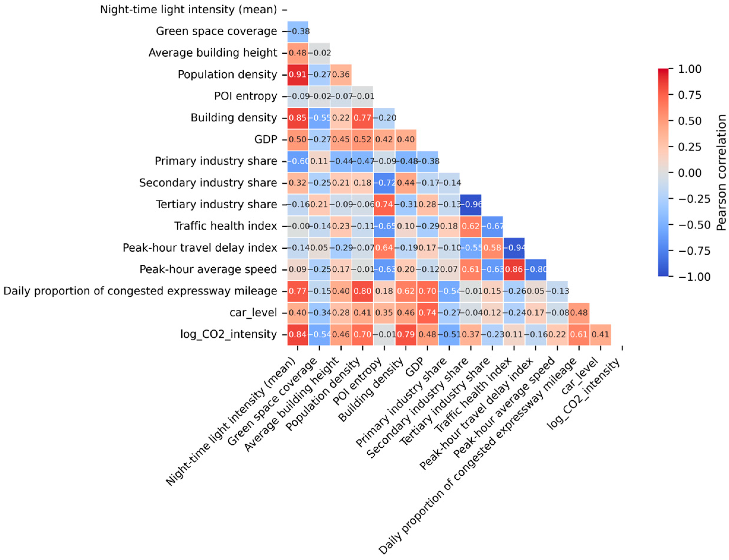
Figure 8 presents the Pearson correlation matrix for all variables. Several built-environment and economic indicators—particularly night-time light intensity, population density, building density, and the tertiary-industry share—exhibit positive correlations with log-transformed CO₂ emission intensity, while primary-industry share is negatively correlated with emissions. Correlations among the explanatory variables are mostly moderate (|r| < 0.6), suggesting that multicollinearity is unlikely to distort the subsequent modelling results. Overall, the descriptive patterns point to a multifaceted relationship between urban development, transport performance, and carbon emissions, underscoring the need for a modelling approach capable of capturing nonlinear effects and interaction structures.

4.2. Performance of the Global XGBoost Model

The global XGBoost model demonstrates a reasonably strong ability to reproduce the spatial variation in urban CO₂ emission intensity. As reported in

Table 6. XGBoost global metrics.

Factor	Value
Five-fold CV R2	0.5491, 0.8496, 0.5058, 0.5205, 0.7919
Mean CV R2	0.6433
Test R2	0.5634
Test RMSE	0.9365
Test MAE	0.5149

, the five-fold cross-validation yields R² values ranging from 0.51 to 0.85, with a mean CV R² of 0.6433, indicating that the model captures a substantial proportion of variability across folds. The held-out test set further confirms the model’s predictive reliability, achieving a test R² of 0.5634, an RMSE of 0.9365, and an MAE of 0.5149.

Although the test R² is slightly lower than the average cross-validation score, the consistency in magnitude suggests that the model does not suffer from severe overfitting and retains stable generalisation capability. Given the multidimensional and nonlinear nature of the determinants—including transport performance, built-environment characteristics, and socioeconomic conditions—these results indicate that XGBoost provides an appropriate modelling framework for capturing complex emission–urban form–mobility interactions at the city scale.

4.3. Global Feature Importance

Figure 9 indicates the relative contributions of the explanatory variables in the global XGBoost model. Night-time light intensity emerges as the most influential predictor, indicating a strong link between urban activity intensity and carbon-emission levels. Built-environment variables—particularly building density and population density—form the next tier of influential factors, suggesting that more compact and densely developed cities tend to exhibit higher emission intensity.

Industrial-structure indicators contribute more modestly: primary-industry share shows a noticeable but smaller effect, whereas secondary- and tertiary-industry shares play only minor roles. Transport-related variables, including congestion, average speed, and traffic health, receive comparatively low importance scores. Their limited contribution at the cross-city level implies that structural economic and spatial characteristics exert greater influence on emission differences than traffic performance alone.

4.4. Nonlinear Effects and Threshold Patterns

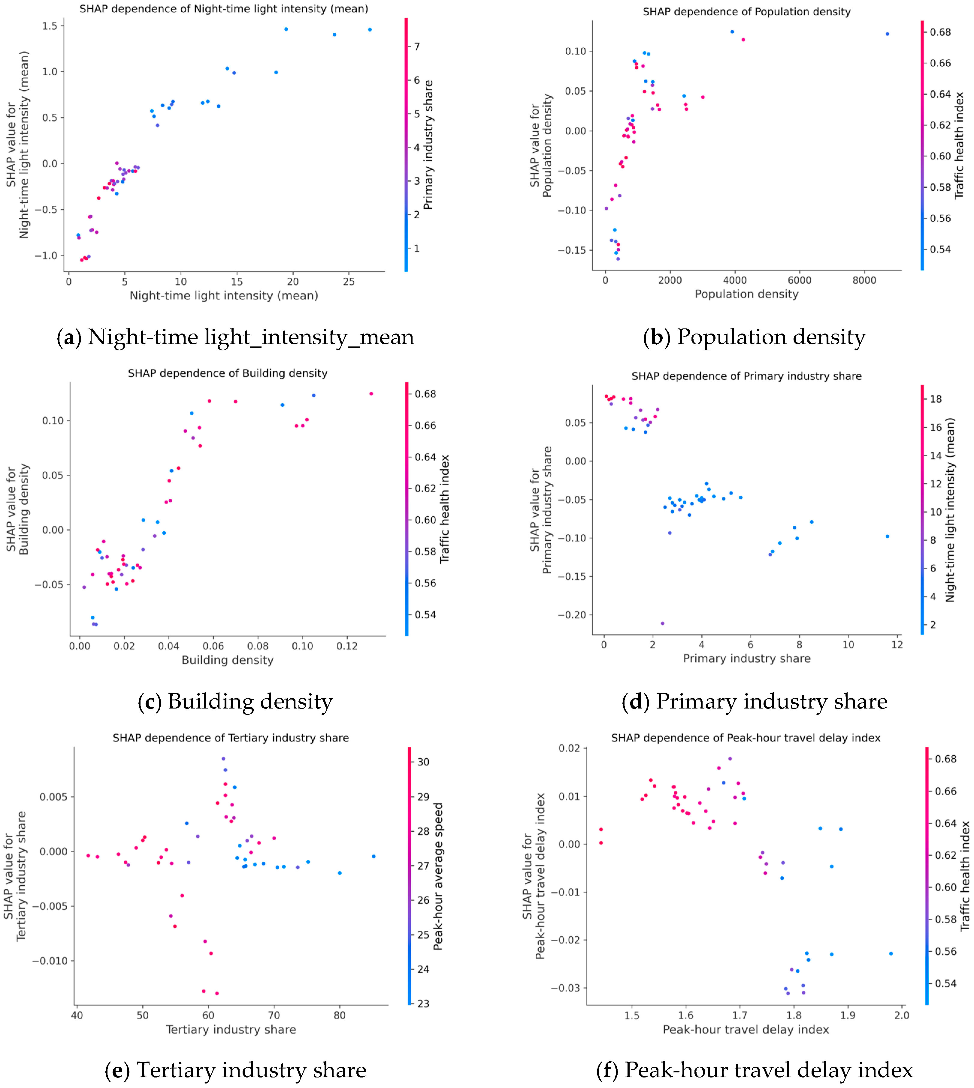
The SHAP dependence plots in Figure 10 illustrate distinct nonlinear patterns across the key variables. Night-time light intensity (Figure 10a) shows a rapid rise in contribution at lower values, followed by a levelling-off at higher levels. Population density (Figure 10b) and building density (Figure 10c) exhibit similar shapes, where increases in their lower-to-middle ranges are associated with higher SHAP values, while changes at the upper end have smaller effects.

Primary-industry (Figure 10d) share displays a generally negative relationship with emission intensity, with stronger marginal reductions at low shares. Tertiary-industry share (Figure 10e) shows only weak and dispersed patterns, consistent with its low global importance. The peak-hour travel delay index (Figure 10f) does not follow a single trend: contributions vary across the range, with positive values around moderate congestion and more scattered responses at higher delays. These patterns show that the effects of activity intensity, urban density, and congestion vary across different parts of their distributions rather than following linear shifts.

From a mechanistic perspective, these nonlinear patterns are consistent with the idea that urban emission responses evolve across different development stages. At lower levels of activity and density, increases in population concentration and mobility demand tend to induce substantial growth in energy use and emissions. As cities become denser and more congested, however, marginal increases in activity or built intensity generate smaller proportional emission changes, reflecting saturation effects related to network capacity constraints, behavioural adaptation, and infrastructural limits. Similar nonlinear or diminishing-return relationships between density, congestion, and emissions have been reported in previous studies [9,12,20].

4.5. Congestion-Based Heterogeneity Analysis

Cities were divided into low- and high-congestion groups using the median peak-hour travel delay index. Model performance differs across the two groups, and its cross-validation scores are also more consistent (

Table 7. XGBoost group metrics with low- and high-congestion groups.

Group	Number of Samples	cv_r2_Mean	Test_r2	Test_Rmse	Test_Mae
low	25	0.6984	0.801	0.3602	0.3166
high	25	0.5772	0.6991	0.3757	0.3108

): the low-congestion model attains a higher test R² (0.80) than the high-congestion model (0.70). This indicates that emission patterns are easier to capture in cities where traffic conditions are relatively smooth, while stronger variability in the high-congestion group suggests more complex interactions among traffic delays, urban form, and activity intensity.

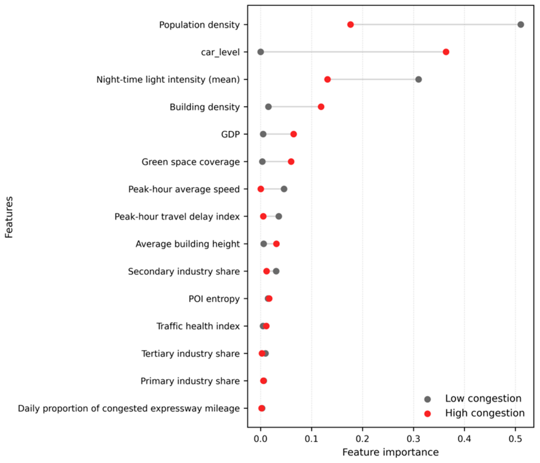
The feature-importance comparison in Figure 11 shows clear shifts across congestion regimes. Population density, car ownership level, and building density contribute more strongly in the high-congestion group, indicating a greater sensitivity of emissions to spatial and demographic pressures under heavy congestion. In contrast, night-time light intensity retains higher importance in the low-congestion group, where its association with emission intensity appears more consistent. These differences point to congestion as an important factor shaping how urban form and activity patterns relate to emissions.

This congestion-dependent shift in driver importance suggests that congestion functions as a regime condition rather than a simple additive factor. In relatively uncongested cities, emissions scale more directly with overall activity intensity, which is consistent with findings from studies assuming near-linear activity–emission relationships [9,12]. In highly congested cities, by contrast, population distribution, motorisation level, and built-form intensity become more influential, indicating that congestion amplifies the carbon consequences of spatial concentration and inefficient travel conditions, as also observed in transport-focused emission studies [20,21].

4.6. Grid-Level Spatial Heterogeneity Based on GNNWR

To uncover intra-urban heterogeneity that is masked in the city-level analysis, we conduct a 1 km grid analysis using GNNWR to estimate spatially varying local coefficients. Methodologically, GNNWR can be viewed as a GeoAI-oriented spatial learning approach, as it integrates graph-based representation of neighbourhood connectivity with geographically weighted modelling to characterise nonstationary relationships. This section therefore reports the grid-level spatial patterns and mechanism interpretation, including dominant drivers by city type, the strength and dispersion of local effects, and representative coefficient maps.

4.6.1. Typology of Cities and Dominant Drivers

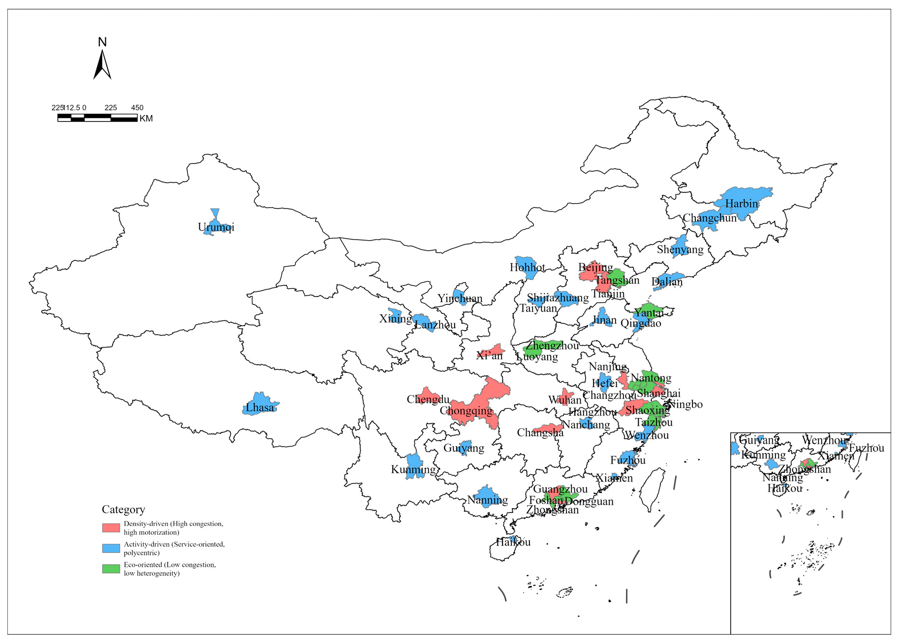
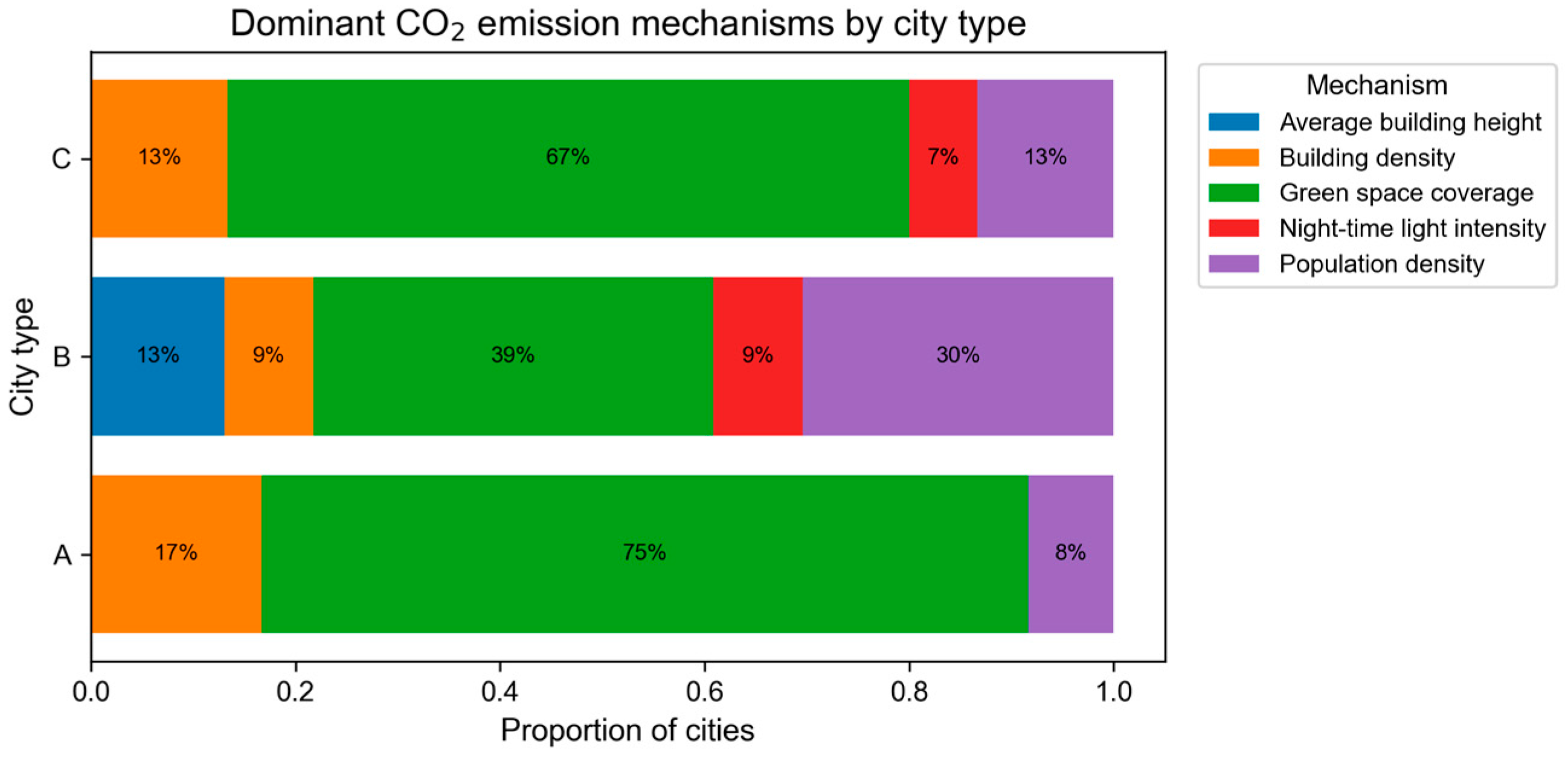
Figure 12 indicates that the importance ranking of predictors varies across congestion regimes. To synthesise these differences, cities are grouped into three types according to the relative prominence of the pre-defined density, activity, and green indices, each representing a distinct dominant mechanism of spatial heterogeneity. Compared with low-congestion cities, the high-congestion group exhibits a clearer role of density- and pressure-related factors, suggesting that the links between urban form and CO₂ intensity differ systematically across urban regimes. Accordingly, the grid-level GNNWR results are summarised by city type.

In Figure 13, green space coverage is the most common dominant driver in Types A and C, accounting for 75% of Type A and 67% of Type C cities. In Type A, the remaining cities are mainly dominated by building density (17%) and population density (8%). In Type C, building density and population density each account for 13%, while night-time light intensity contributes 7%. By contrast, Type B shows a more mixed driver structure. Green space coverage remains the most frequent dominant mechanism (39%), but population density (30%) is nearly as common, and average building height (13%), together with building density (9%) and night-time light intensity (9%), also emerge as dominant drivers. Overall, Type B is characterised by a more diversified mechanism mix, whereas Types A and C are more consistently green-space-dominated.

These typological differences highlight that similar city-level emission drivers may arise from fundamentally different intra-urban mechanisms. In density-driven cities, dominant effects tend to be concentrated in specific cores or corridors, whereas in activity-driven cities, emission mechanisms are more fragmented across multiple subareas. This finding extends existing city-level studies by demonstrating that heterogeneity is not only inter-city but also strongly intra-urban, which has been largely overlooked in previous cross-city emission analyses [9,12,20].

When cities move from the low- to high-congestion regime, the explanatory weight shifts towards density- and pressure-related factors, implying that the emission–urban form relationship becomes more sensitive to crowding and built intensity. Against this background, the dominant-mechanism composition by type provides a compact interpretation: Types A and C are characterised by a relatively stable dominance of green-space-related effects, suggesting that within these regimes the spatial distribution of green infrastructure aligns most consistently with the spatial variation in emission intensity. Type B, in contrast, concentrates the regime where dominant drivers become diversified, meaning that no single mechanism is sufficient to represent the citywide pattern and that local effects are more likely to vary across different urban contexts within the same city.

4.6.2. Spatial Heterogeneity of Local Coefficients Across City Types

Figure 14 summarises the within-city dispersion of local GNNWR coefficients using the standard deviation of $\beta$. For both population density and building density, Types A and C generally exhibit broader spreads than Type B, indicating stronger intra-urban non-stationarity in density-related effects under these regimes. In contrast, the dispersion of POI entropy is overall smaller, but Type C shows a longer upper tail, suggesting that functional-mix effects become locally pronounced only in specific subareas rather than being expressed uniformly across the city.

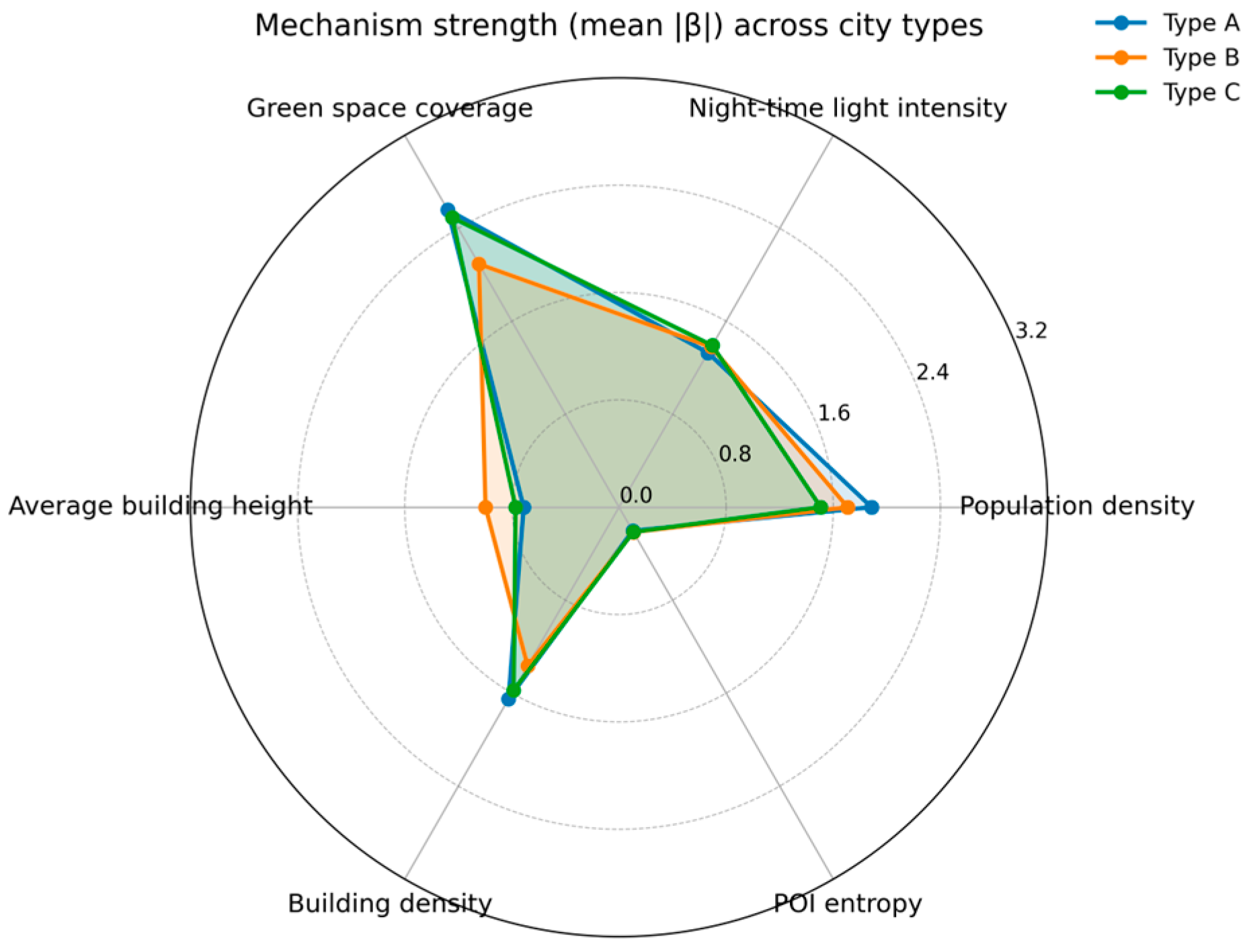
Complementing the dispersion statistics, the radar plot (Figure 15) compares the average mechanism strength across city types using the mean of $\mid \beta \mid$. Across all three types, green space coverage shows the largest mean $\mid \beta \mid$, followed by density-related mechanisms, whereas POI entropy remains consistently weak in magnitude. Differences across types are also evident: Type A shows relatively stronger associations with population density and building density, while Type B presents more balanced strengths across activity- and density-related mechanisms; Type C is characterised by a strong green-space signal together with comparatively weaker or more localised effects for other drivers.

4.6.3. Representative Cities and Intra-Urban Spatial Patterns

Using the city-type indices, representative cities are selected to illustrate the intra-urban spatial patterns of local coefficients. Specifically, cities with the highest index values within each type are chosen as representative cases for visual comparison. Specifically, Type A candidates were ranked by the density index (selecting the city with the highest density index), Type B candidates were ranked by the activity index (selecting the highest-activity case), and Type C candidates were identified as cities with a low combined intensity of density- and activity-related mechanisms (i.e., a small $density\_index+activity\_index$) but a relatively stronger green-space signal (higher green index). Following this rule, Chengdu, Changchun, and Taizhou were chosen to represent Types A–C, respectively, ensuring that each case reflects the most typical mechanism profile implied by the typology rather than an arbitrary choice.

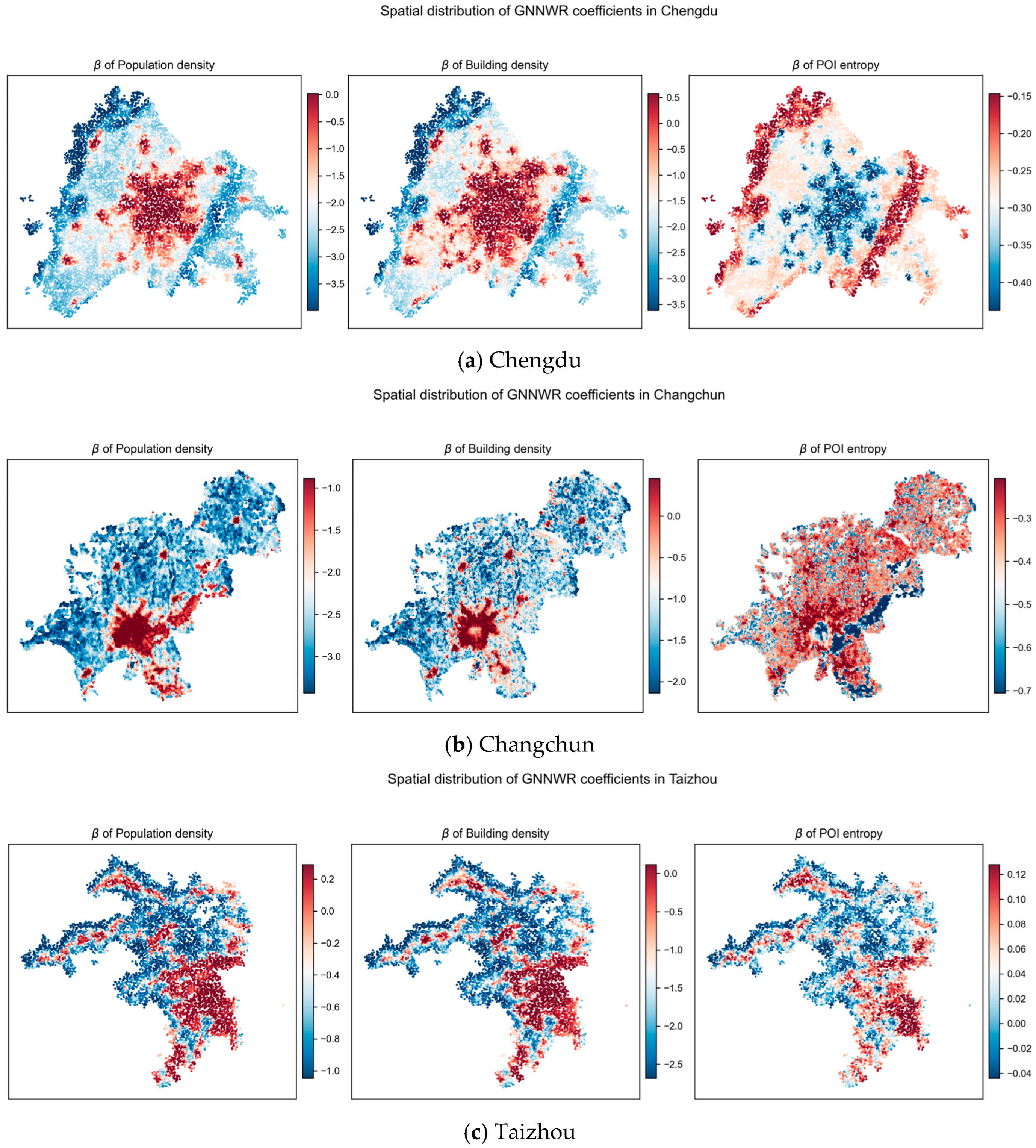
Figure 16 maps the local GNNWR coefficients for population density, building density, and POI entropy in these three cities. The maps show that the typology is expressed as distinct spatial organisations of local effects rather than as simple differences in average values.

In Chengdu (Type A; density-driven) (Figure 16a), the density-related coefficients ($\beta$ for population density and building density) form a strong, spatially concentrated signal. High-magnitude coefficients cluster in the main built-up core and extend along major development corridors, while outer areas exhibit markedly weaker effects. This pattern indicates that the “density-driven” label is not generated by uniform citywide sensitivity but by a set of high-intensity zones where densification is tightly coupled with emission intensity. The coefficient surface of POI entropy is comparatively discontinuous, suggesting that functional-mix effects are locally relevant but secondary to the dominant density mechanism in most areas.

In Changchun (Type B; activity-driven) (Figure 16b), the coefficient surfaces are more spatially fragmented and differ more strongly across variables. Pockets of higher-magnitude coefficients appear across multiple separated subareas rather than being anchored by a single dominant core. This spatial patchwork is consistent with the Type B mechanism profile derived from the indices and the dominant-driver statistics: different urban substructures are governed by different mechanisms, so the city-level summary emerges from competing local processes rather than from one coherent driver.

In Taizhou (Type C; low-heterogeneity/eco-oriented) (Figure 16c), the density-related coefficient magnitudes are generally less extreme, and the spatial pattern is smoother. Compared with Chengdu and Changchun, the maps show fewer sharply bounded hotspots and more continuous areas with moderate coefficients. This matches the selection criterion for Type C—low combined density/activity intensity but a relatively stronger green-space signal—and suggests that the dominant city-level mechanism is supported by more evenly distributed local effects, rather than by isolated high-intensity urban zones.

Overall, the representative-city maps provide a concrete spatial validation of the index-based typology. Type A is characterised by concentrated density hotspots, Type B by multi-zone competition among mechanisms, and Type C by comparatively weak and smoother spatial contrasts. These results explain why the same “dominant driver” at the city level can arise either from a few strong clusters or from widespread moderate effects. Compared with previous studies that rely primarily on administrative averages, these spatial patterns offer direct evidence that emission mechanisms operate unevenly within cities, thereby reinforcing the need for spatially explicit approaches to low-carbon planning and transport–land-use coordination.

These results provide insights into the mechanisms through which transport conditions and the built environment influence urban CO₂ emission intensity. At the city level, built-environment attributes such as population density, building density, and functional mix shape travel demand and activity concentration, thereby affecting trip frequency, travel distance, and mode choice. In contrast, transport-related indicators such as congestion and operating speed primarily capture short-term efficiency losses and therefore exhibit weaker explanatory power in cross-city comparisons, indicating that structural urban form exerts a more persistent influence on emission differences.

At the intra-urban scale, the GNNWR results further reveal pronounced spatial heterogeneity in these mechanisms. In highly congested cities, density- and pressure-related factors tend to dominate in central urban areas, while peripheral zones display more heterogeneous or attenuated effects. This finding is consistent with previous studies emphasising the role of urban form in shaping transport-related emissions, and it extends existing evidence by demonstrating that similar city-level emission patterns may arise from distinct local processes, underscoring the importance of spatially explicit analysis.

5. Conclusions

This study investigates the determinants of CO₂ emission intensity across fifty major Chinese cities by integrating transport conditions, built-environment structure, socioeconomic characteristics, and night-time light intensity. To move beyond linear “average-city” assumptions, we develop a GeoAI-oriented workflow that combines XGBoost for nonlinear modelling, SHAP for interpretable mechanism diagnosis, congestion-based city grouping for regime comparison, and 1 km grid-level GNNWR for mapping intra-urban spatial non-stationarity. Together, these components provide a multi-scale understanding of how mobility conditions and urban form jointly shape emission outcomes.

Three main conclusions can be drawn. First, activity intensity and development concentration explain most of the cross-city variation in CO₂ emission intensity. In the global model, night-time light intensity is the strongest predictor, followed by population density and building density. SHAP dependence patterns reveal pronounced nonlinearities: emissions are highly sensitive to increases in activity and density at low–medium levels, but marginal effects diminish as cities become more active and denser. This suggests that the emission response to urbanisation is not proportional and that the same increment in intensity may correspond to very different emission changes across the distribution.

Second, congestion functions as a regime condition that reshapes emission mechanisms rather than acting as a simple additive factor. Although transport indicators appear less influential in the aggregate model, their roles and interactions change markedly across congestion regimes. In low-congestion cities, emission intensity aligns more consistently with overall activity intensity, indicating a relatively direct activity–emission linkage when traffic operates more smoothly. In high-congestion cities, emissions become more sensitive to population distribution, motorisation level, and built-form intensity, and the relationships are less stable, consistent with a setting where congestion alters travel efficiency and strengthens the coupling between spatial structure and mobility-related emissions. These results indicate that mitigation levers differ systematically across mobility contexts.

Third, emission mechanisms are spatially uneven within cities, and city-level drivers can arise from different intra-urban spatial organisations. Grid-level GNNWR results show clear non-stationarity: in some cities, density-related effects concentrate in specific cores and corridors, while in others the dominant mechanisms are more fragmented across multiple subareas or exhibit smoother spatial contrasts with a stronger green-space signal. This intra-urban heterogeneity implies that citywide averages may hide high-impact zones and that planning interventions should be spatially targeted rather than uniformly applied.

The findings support differentiated strategies. For relatively uncongested cities, policies that improve energy efficiency of activity and moderate high-intensity expansion may yield clearer emission benefits. For highly congested cities, measures that address spatial structure and motorisation dependence are likely to be more effective, including congestion-sensitive land-use planning, corridor- and centre-focused intensity management, and interventions that reduce peak-hour pressure through improved jobs–housing alignment and multimodal accessibility. At the intra-urban scale, GNNWR-based heterogeneity mapping provides a practical basis for prioritising where interventions should be targeted—whether toward a small set of density–emission hotspots or toward broader, citywide form- and green-infrastructure adjustments.

This study is cross-sectional and cannot capture dynamic feedback among congestion, land development, and emissions over time. Transport indicators are primarily city-level and may not fully reflect within-city travel patterns or freight activity. Future work could incorporate multi-year panel data, finer-grained mobility measures (e.g., OD flows, mode shares, and freight proxies), and scenario-based evaluation of land-use and transport interventions to strengthen causal interpretation and improve policy testing.

References

- Wu, J.; Jia, P.; Feng, T.; Li, H.; Kuang, H. Spatiotemporal analysis of built environment restrained traffic carbon emissions and policy implications. Transp. Res. Part D Transp. Environ. 2023, 121, 103839. [Google Scholar] [CrossRef]
- Jia, C.; Wang, X.; Qian, C.; Cao, Z.; Zhao, L.; Lin, L. Quantitative study on the environmental impact of Beijing’s urban rail transit based on carbon emission reduction. Sci. Rep. 2025, 15, 2380. [Google Scholar] [CrossRef]
- Zhang, N.; Luo, Z.; Liu, Y.; Feng, W.; Zhou, N.; Yang, L. Towards low-carbon cities through building-stock-level carbon emission analysis: A calculating and mapping method. Sustain. Cities Soc. 2022, 78, 103633. [Google Scholar] [CrossRef]
- Jin, G.; Wang, G.; Li, W.; Sheng, H.; Hu, C.; Zhao, Y. The impact of environmental regulation on carbon emissions and its mechanisms in Chinese cities. Sci. Rep. 2025, 15, 41665. [Google Scholar] [CrossRef]
- Zhang, H.-S.; Xu, N.; Zhang, S.; Hu, W.; Deng, C.; Chang, Y.; Zhang, Z.; Ou, Y. The hidden economic costs of air pollution in China: Evidence from remotely sensed nighttime light data. GISci. Remote Sens. 2025, 62, 2546167. [Google Scholar] [CrossRef]
- Ling, C.; Tang, J.; Zhao, P.; Xu, L.; Lu, Q.; Yang, L.; Huang, F.; Lyu, W.; Yang, J. Unraveling the relation between carbon emission and carbon footprint: A literature review and framework for sustainable transportation. npj Sustain. Mobil. Transp. 2024, 1, 13. [Google Scholar] [CrossRef]
- Zhao, L.; He, Z. Using machine learning to analyze the factors influencing city-level transportation carbon emissions. Energy 2025, 333, 137355. [Google Scholar] [CrossRef]
- Li, S.; Zhang, X.; Deng, Z.; Liu, K.; Wang, J.; Fan, J. Widening inequality: Diverging trends in CO2 and air pollutant emissions across Chinese cities. Resour. Environ. Sustain. 2025, 21, 100227. [Google Scholar] [CrossRef]
- Zhang, A.; Li, W.; Xia, C.; Guo, H. The impact of urban landscape patterns on land surface temperature at the street block level: Evidence from 38 big Chinese cities. Environ. Impact Assess. Rev. 2025, 110, 107673. [Google Scholar] [CrossRef]
- Yang, Y.; Ouyang, L.; Wu, Z.; Jiang, Q.M.; Qiao, R. Nonlinear effects of urban multidimensional characteristics on air pollution heterogeneity in China’s urban agglomerations. J. Clean. Prod. 2025, 491, 144813. [Google Scholar] [CrossRef]
- Ou, Y.; Zheng, J.; Liang, Y.; Bao, Z. When green transportation backfires: High-speed rail’s impact on transport-sector carbon emissions from 315 Chinese cities. Sustain. Cities Soc. 2024, 114, 105770. [Google Scholar] [CrossRef]
- Gao, X.; Wang, H.; Zhang, Y.; Cao, M. Understanding the spatial differentiation and spatiotemporal mechanisms of carbon emissions from urban transport. Cities 2025, 167, 106380. [Google Scholar] [CrossRef]
- Xing, X.; Xi, Q.; Shi, W. Impact of urban compactness on carbon emission in Chinese cities: From moderating effects of industrial diversity and job-housing imbalances. Land Use Policy 2024, 143, 107213. [Google Scholar] [CrossRef]
- Huang, X. Geospatial Artificial Intelligence (GeoAI) Is Widening the Digital Divide. Ann. Am. Assoc. Geogr. 2025, 115, 2017–2029. [Google Scholar] [CrossRef]
- Liu, D.; Wang, R.; Grekousis, G.; Liu, Y.; Lu, Y. Detecting older pedestrians and aging-friendly walkability using computer vision technology and street view imagery. Comput. Environ. Urban Syst. 2023, 105, 102027. [Google Scholar] [CrossRef]
- Lu, F.; Cheng, S.; Wang, P. GeoAI enabled urban computing: Status and challenges. Ann. GIS 2025, 31, 537–555. [Google Scholar] [CrossRef]
- Liu, D.; Lu, Y.; Yang, L. Exploring non-linear effects of environmental factors on the volume of pedestrians of different ages using street view images and computer vision technology. Travel Behav. Soc. 2024, 36, 100814. [Google Scholar] [CrossRef]
- Huang, G.; Li, D.; Ng, S.T.; Wang, L.; Zhang, Y. Vision-based personal thermal comfort modeling under facial occlusion scenarios. Energy Build. 2025, 335, 115566. [Google Scholar] [CrossRef]
- Mai, G.; Xie, Y.; Jia, X.; Lao, N.; Rao, J.; Zhu, Q.; Liu, Z.; Chiang, Y.-Y.; Jiao, J. Towards the next generation of Geospatial Artificial Intelligence. Int. J. Appl. Earth Obs. Geoinf. 2025, 136, 104368. [Google Scholar] [CrossRef]
- Huang, Z.; Loo, B.P.Y. Urban traffic congestion in twelve large metropolitan cities: A thematic analysis of local news contents, 2009–2018. Int. J. Sustain. Transp. 2022, 17, 592–614. [Google Scholar] [CrossRef]
- Li, X.; Sinniah, G.K.; Li, R.; Li, X. Correlation between Land Use Pattern and Urban Rail Ridership Based on Bicycle-Sharing Trajectory. ISPRS Int. J. Geo-Inf. 2022, 11, 589. [Google Scholar] [CrossRef]
- Li, X.Y.; Sinniah, G.K.; Li, R. Identify impacting factor for urban rail ridership from built environment spatial heterogeneity. Case Stud. Transp. Policy 2022, 10, 1159–1171. [Google Scholar] [CrossRef]
- Yao, W.; Shen, X.; He, Z.; Liu, Y.; Yang, X.; Zeng, J.; Zhang, C.; Jin, S. Unlocking the potential of cooperative staggered shifts in urban networks. Transp. Res. Part C Emerg. Technol. 2025, 180, 105354. [Google Scholar] [CrossRef]
- Tian, Z.; Zhao, Y.; Dong, Z.; Sun, D.J.; Dong, Z. Analyzing the spatiotemporal heterogeneity of carbon emissions from road transportation in four Chinese urban agglomerations: An empirical case study. Transp. Policy 2025, 173, 103756. [Google Scholar] [CrossRef]
- Weng, D.; Zhang, H.; Wen, X.; Hu, X.; Zhang, L. Co-benefits of carbon and pollutant emission reduction in urban transport: Sustainable pathways and economic efficiency. Urban Clim. 2025, 60, 102348. [Google Scholar] [CrossRef]
- Wang, H.; Shi, W.; He, W.; Xue, H.; Zeng, W. Simulation of urban transport carbon dioxide emission reduction environment economic policy in China: An integrated approach using agent-based modelling and system dynamics. J. Clean. Prod. 2023, 392, 136221. [Google Scholar] [CrossRef]
- Malekzadeh, M.; Smith, L.; Reuschke, D.; Farber, S.; Long, J. Urban mobility and carbon emissions: Decoding the influence of sociodemographic factors, trip-level built environment, and travel behaviour of workers in three UK cities. Cities 2025, 167, 106321. [Google Scholar] [CrossRef]
- Shang, W.-L.; Song, X.; Chen, Y.; Yang, X.; Liang, L.; Deveci, M.; Cao, M.; Xiang, Q.; Yu, Q. Congestion and Pollutant Emission Analysis of Urban Road Networks Based on Floating Vehicle Data. Urban Clim. 2024, 53, 101794. [Google Scholar] [CrossRef]
- Jiang, Y.; Chen, L.; Grekousis, G.; Xiao, Y.; Ye, Y.; Lu, Y. Spatial disparity of individual and collective walking behaviors: A new theoretical framework. Transp. Res. Part D Transp. Environ. 2021, 101, 103096. [Google Scholar] [CrossRef]
- Ou, Y.; Lee, S.Y.; Nam, K.M.; Lee, K. Rethinking post-pandemic urban planning strategies: Lessons from Singapore and Hong Kong. J. Korea Plan. Assoc. 2023, 58, 27–47. [Google Scholar] [CrossRef]
- Ou, Y.; Bao, Z.; Ng, S.T.; Song, W.; Chen, K. Land-use carbon emissions and built environment characteristics: A city-level quantitative analysis in emerging economies. Land Use Policy 2024, 137, 107019. [Google Scholar] [CrossRef]
- Jiang, Y.; Liu, D.; Ren, L.; Grekousis, G.; Lu, Y. Tree abundance, species richness, or species mix? Exploring the relationship between features of urban street trees and pedestrian volume in Jinan, China. Urban For. Urban Green. 2024, 95, 128294. [Google Scholar] [CrossRef]
- Liu, M.; Zhu, X. Mismatch between objective and subjective livability assessment: A case study in Hong Kong. Urban Inform. 2025, 4, 22. [Google Scholar] [CrossRef]
- Nassar, R.; Napier-Linton, L.; Gurney, K.R.; Andres, R.J.; Oda, T.; Vogel, F.R.; Deng, F. Improving the temporal and spatial distribution of CO2 emissions from global fossil fuel emission data sets. J. Geophys. Res. Atmos. 2013, 118, 917–933. [Google Scholar] [CrossRef]
- Oda, T.; Maksyutov, S.; Andres, R.J. The Open-source Data Inventory for Anthropogenic CO2, version 2016 (ODIAC2016): A global monthly fossil fuel CO2 gridded emissions data product for tracer transport simulations and surface flux inversions. Earth Syst. Sci. Data 2018, 10, 87–107. [Google Scholar] [CrossRef] [PubMed]
- Hsu, F.-C.; Baugh, K.; Ghosh, T.; Zhizhin, M.; Elvidge, C. DMSP-OLS Radiance Calibrated Nighttime Lights Time Series with Intercalibration. Remote Sens. 2015, 7, 1855–1876. [Google Scholar] [CrossRef]
- Elvidge, C.D.; Baugh, K.; Zhizhin, M.; Hsu, F.C.; Ghosh, T. VIIRS night-time lights. Int. J. Remote Sens. 2017, 38, 5860–5879. [Google Scholar] [CrossRef]
- Yang, J.; Huang, X. The 30 m annual land cover dataset and its dynamics in China from 1990 to 2019. Earth Syst. Sci. Data 2021, 13, 3907–3925. [Google Scholar] [CrossRef]
- Che, Y.; Li, X.; Liu, X.; Wang, Y.; Liao, W.; Zheng, X.; Zhang, X.; Xu, X.; Shi, Q.; Zhu, J.; et al. 3D-GloBFP: The first global three-dimensional building footprint dataset. Earth Syst. Sci. Data 2024, 16, 5357–5374. [Google Scholar] [CrossRef]
- Ju, Y.; Liang, Y.; Kong, J.; Wang, X.; Wen, S.; Shang, H.; Wang, X. 100-m resolution Age-Stratified Population Estimation from the 2020 China Census by Township (ASPECT). Sci. Data 2025, 12, 1058. [Google Scholar] [CrossRef]
- Zhang, T.; Tang, F.; Hu, Y.; Zhang, L.; Guo, Y. Shaping greener mobility: Impact of urban greening structure on time-dependent bike-sharing usage. Transp. Res. Part D Transp. Environ. 2025, 141, 104657. [Google Scholar] [CrossRef]
- Wang, L.; Yang, J.; Wu, S.; Hu, L.; Ge, Y.; Du, Z. Enhancing mineral prospectivity mapping with geospatial artificial intelligence: A geographically neural network-weighted logistic regression approach. Int. J. Appl. Earth Obs. Geoinf. 2024, 128, 103746. [Google Scholar] [CrossRef]
- Ni, S.; Wang, Z.; Wang, Y.; Wang, M.; Li, S.; Wang, N. Spatial and Attribute Neural Network Weighted Regression for the Accurate Estimation of Spatial Non-Stationarity. ISPRS Int. J. Geo-Inf. 2022, 11, 620. [Google Scholar] [CrossRef]
- Wu, S.; Wang, Z.; Du, Z.; Huang, B.; Zhang, F.; Liu, R. Geographically and temporally neural network weighted regression for modeling spatiotemporal non-stationary relationships. Int. J. Geogr. Inf. Sci. 2020, 35, 582–608. [Google Scholar] [CrossRef]
Figure 2.
Conceptual framework.
Figure 3.
ODIAC CO2 emission at grid level.
Figure 4.
VIIRS night-time light in study area.
Figure 5.
Land-cover dataset in study area (Hangzhou city).
Figure 6.
3D-GloBFP building dataset in study area (Hangzhou city).
Figure 7.
Population density (100 m) in study area (Hangzhou city).
Figure 8.
Correlation matrix.
Figure 9.
Shap summary global.
Figure 10.
SHAP dependence plots of key explanatory variables.
Figure 11.
Feature importance dumbbell, low- and high-congestion groups.
Figure 12.
Predictor importance rankings across congestion regimes.
Figure 13.
Dominant mechanism by city type.
Figure 14.
Spatial heterogeneity boxplots.
Figure 15.
Comparison of mechanism strength across city types.
Figure 16.
Spatial distribution of selected GNNWR coefficients in representative cities.